Model Criticism in Latent Space

Abstract

Model criticism is usually carried out by assessing if replicated data generated under the fitted model looks similar to the observed data, see e.g. Gelman, Carlin, Stern, and Rubin (2004, p. 165). This paper presents a method for latent variable models by pulling back the data into the space of latent variables, and carrying out model criticism in that space. Making use of a model’s structure enables a more direct assessment of the assumptions made in the prior and likelihood. We demonstrate the method with examples of model criticism in latent space applied to factor analysis, linear dynamical systems and Gaussian processes.

1 Introduction

Model criticism is the process of assessing the goodness of fit between some data and a statistical model of that data. While model criticism uses goodness-of-fit tests to judge aspects of the model, its general objective is to identify deficiencies in the model that can lead to model extension to address these deficiencies. The extended model(s) can again be subjected to criticism, and the process continues until a satisfactory model is found (O’Hagan, 2003). Model criticism is contrasted with model comparison in that model criticism assesses a single model, while model comparison deals with at least two models to decide which model is a better fit. Model comparison can be applied to compare the original and the extended model after model criticism and extension (O’Hagan, 2003, p. 2).

Bayesian modelling has become an indispensable tool in statistical learning, and it is being widely used to model complex signals, e.g., by Ratmann et al. (2009). With its growing popularity, there is need for model criticism in this framework. Most work on model criticism makes use of the idea that “if the model fits, then replicated data generated under the model should look similar to observed data” (Gelman et al., 2004, p. 165). In contrast, in this paper we focus on a less well explored idea that for latent variable models, we can probabilistically pull back the data into the space of the latent variables, and carry out model criticism in that space. We can summarize this principle as that if the model fits, then posterior inferences should match the prior assumptions.

To elaborate, consider a model with observed variables $X$ and unobserved variables $U$ with joint distribution $P(X,U\,|\,\gamma)$ where $\gamma$ are known parameters. In general $U$ may contain latent variables $Z$, parameters $\Theta$, and hyperparameters $\lambda$. Given a sample $x^{\mathrm{obs}}$ from the marginal distribution $P(X\,|\,\gamma)$, and a single posterior sample $u^{\ast}$ from the conditional distribution $P(U\,|\,x^{\mathrm{obs}},\gamma)$, the joint sample $(x^{\mathrm{obs}},u^{\ast})$ is a draw from the distribution $P(X,U\,|\,\gamma)$. This property can be used to check the fit of the model in the latent space by checking if $u^{\ast}$ is a sample from the marginal distribution $P(U\,|\,\gamma)$. Testing a single sample against a distribution, however, is not an effective approach. But, in many widely-used models, groups of unknown variables are independently and identically distributed under the prior. These related variables are easily aggregated together, giving a simple test of the prior assumptions. Figure 1 summarizes the overall approach, which is justified in §3.

In comparison to model criticism in the observation space, comparing $u^{\ast}$ with prior $P(U\,|\,\gamma)$, provides an additional tool for model criticism which does not require crafting an appropriate discrepancy measure, generating replicate observations, and approximating the null distribution. This approach also does not suffer from the “double use” of data (see discussion in §2). These points have also been made by Yuan and Johnson (2012), but were applied to a relatively small scale hierarchical linear model. We develop the use of model criticism in latent space for large scale and complex models, yielding new insights and developments. Specifically, we apply this approach to the criticism of linear dynamical systems, factor analysis and Gaussian processes, and discuss its connection to the observation space based approach.

The structure of the rest of the paper is as follows: in §2 we describe the methods of model criticism in observation space. §3 provides details of the argument for model criticism in latent space and describes related work, and §4 shows results from applying the method to the three examples. Table 1 describes the notations followed in the paper, and Table 2 shows the distributions used in the paper.

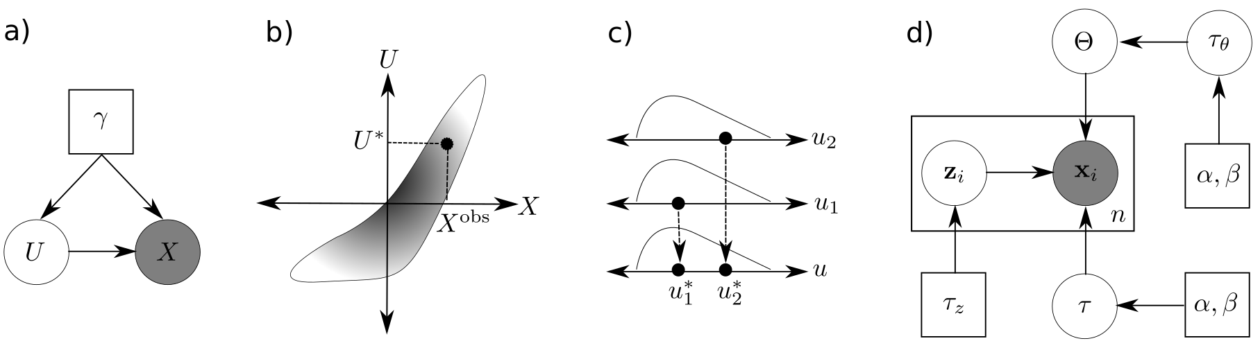
Figure 1: a) A probabilistic model with observed variables $X$, unobserved variables $U$, and known parameters $\gamma$, b) Given the observed data $x^{\mathrm{obs}}$ from $P(X\,|\,\gamma)$ and a posterior sample $u^{\ast}$ from $P(U\,|\,x^{\mathrm{obs}},\gamma)$, $(x^{\mathrm{obs}},u^{\ast})$ is a joint sample from $P(X,U\,|\,\gamma)$, and therefore, $u^{\ast}$ is a sample from $P(U\,|\,\gamma)$ and $x^{\mathrm{obs}}$ is a sample from $P(X\,|\,u^{\ast},\gamma)$. c) If the prior (or part of it) factorizes into identical distributions, e.g., $P(U\,|\,\gamma)\!=\!\prod_{k=1}^{2}P_{u}(U_{k}\,|\,\gamma)$, then posterior sample $\{u_{1}^{\ast},u_{2}^{\ast}\}$ is independent and identical sample from $P_{u}(\cdot\,|\,\gamma)$. d) A factor analysis model showing observed variables $X\!=\!\{\mathbf{x}_{i}\}_{i=1}^{n}$, unobserved variables $U\!=\!\{\{\mathbf{z}_{i}\}_{i=1}^{n},\Theta,\tau,\tau_{\theta}\}$, and known parameters $\gamma\!=\!\{\alpha,\beta,\tau_{z}\}$. We test if $\{z_{11}^{\ast},z_{12}^{\ast},\ldots\}$ is a sample from $P(Z\,|\,\tau_{z})$, and $\{\theta_{11}^{\ast},\theta_{12}^{\ast},\ldots\}$ is a sample from $P(\theta\,|\,\tau_{\theta}^{\ast})$.

Style	Explanation	Example
Upper case italics	Random variable or a group of random variables	$X,Z,U=\{U_{1},\ldots,U_{K}\}$
Lower case italics	Realization of a random variable	$\{x_{i}\}_{i=1}^{n},u^{\ast}$
Lower case bold	Vectors, realization or random variable	$\{\textbf{x}_{i}\}_{i=1}^{n},P(\mathbf{z}),\mathbf{u}=(u_{1},\ldots,u_{K})^{\top}$
Upper case bold	Matrices, realization or random variable	$\{\mathbf{X}_{i}\}_{i=1}^{n},P(\mathbf{Z}),\mathbf{U}=[\mathbf{u}_{1},\ldots,\mathbf{u}_{K}]$
$P(X)$	Distribution of random variable $X$	$X\sim P(X)$
$P(X\,|\,y)$	Conditional distribution of random variable $X$ given $Y=y$	$X\sim P(X\,|\,y)$
$p(x)$	Probability density function of r. v. $X$, abbreviation for $p_{X}(x)$	$p(y)=\int p(x,y)\textrm{d}x$
$p(x\,|\,y)$	Conditional density function of r. v. $X$ given $Y=y$, abbreviation for $p_{X\,|\,Y}(x\,|\,y)$	$p(y)=\int p(x\,|\,y)p(y)\textrm{d}x$
$\cdot\sim\cdot$	Distributed as	$X^{\mathrm{rep}}\sim P(X),X\sim\mathcal{N}(0,1)$
$\cdot^{\ast}$	A posterior sample	$u^{\ast},\mathbf{z}^{\ast}$
$\cdot^{\mathrm{obs}}$	Observed data	$x^{\mathrm{obs}},X^{\mathrm{obs}}\sim P(X)$
$\cdot^{\mathrm{rep}}$	Replicate data	$x^{\mathrm{rep}},X^{\mathrm{rep}}\sim P(X)$
0	Zero vector	$\textbf{x}\sim\mathcal{N}(\textbf{0},\textbf{I})$
I	Identity matrix	$\textbf{x}\sim\mathcal{N}(\textbf{0},\textbf{I})$

Table 1: Description of notation used in the paper.

Name	Notation	Density
Normal	$\mathcal{N}(x\,|\,\mu,\tau\raisebox{3.96107pt}{$\scriptscriptstyle-\!1$})$	$\frac{{\tau}^{1/2}}{(2\pi)^{1/2}}\exp\left(-(\tau(x-\mu)^{2})/2\right)$
Multivariate normal	$\mathcal{N}(\mathbf{x}\,|\,\boldsymbol{\mu},\boldsymbol{\tau}\raisebox{3.96107pt}{$\scriptscriptstyle-\!1$})$	$\frac{{\mathrm{det}(\boldsymbol{\tau})}^{1/2}}{(2\pi)^{d/2}}\exp\left(-((\mathbf{x}-\boldsymbol{\mu})^{\top}\boldsymbol{\tau}(\mathbf{x}-\boldsymbol{\mu}))/2\right)$
Double exponential	$\mathcal{L}(x\,|\,\mu,\tau)$	$\frac{\tau}{2}\exp(-\tau|x-\mu|)$
Gamma	$\mathrm{Gamma}(x\,|\,\alpha,\beta)$	$\frac{\beta^{\alpha}}{\Gamma(\alpha)}x^{\alpha-1}\exp(-\beta x)$
Dirichlet	$\mathrm{Dir}(\mathbf{x}\,|\,\alpha)$	$\frac{1}{B(\alpha)}{\prod_{i=1}^{K}}x_{i}^{\alpha_{i}-1}$ where $x_{i}\in(0,1)$ and $\sum_{i=1}^{K}x_{i}=1$.

Table 2: List of distributions used in the paper.

2 Model Criticism in Observation Space

A general approach of model criticism is to evaluate if replicated data generated under the (fitted) model looks similar to observed data. Consider that we are modelling observed data $x^{\mathrm{obs}}$ with a latent variable model parameterized by $U$, i.e., we have defined the likelihood $p(x\,|\,u)$ and (optionally) a prior distribution $P(U)$ over potential parameter values. The principle of model criticism in the observation space is to assess if $x^{\mathrm{obs}}$ is a reasonable observation under the proposed model. For example, given the maximum likelihood estimator (or another point estimate) $\hat{u}$ of the parameters, one standard approach is to find the plug-in p-value (Bayarri and Berger, 2000)

$$p_{\textrm{plug-in}}=\textrm{Pr}(D(X^{\mathrm{rep}},\hat{u})>D(x^{\mathrm{obs}},\hat{u})).$$ (1)

Here $D$ is called a discrepancy function and it resembles a test statistic in hypothesis testing, i.e., a larger value rejects the null hypothesis or indicates incompatibility of data and model, and $X^{\mathrm{rep}}$ is a replicate observation generated under the fitted model, i.e., $X^{\mathrm{rep}}\sim P(X\,|\,\hat{u})$.

If the p-value is low, then it implies that the probability of generating a more extreme dataset than the observed data is small, or in other words, the observed data itself is considered extreme relative to the model, and thus, the model does not adequately describe the dataset. In summary, a low p-value rejects the hypothesis that the data is being adequately modelled. The p-value is usually estimated via an empirical average by generating multiple replicates $x^{\mathrm{rep}}_{r}$, $r=1,\ldots,R$, and evaluating

$$\hat{p}_{\textrm{plug-in}}= \frac{1}{R}\sum_{r}\mathbf{1}(D(x^{\mathrm{rep}}_{r},\hat{u})>D(x^{\mathrm{obs}},\hat{u})),$$ (2)

where $x^{\mathrm{rep}}_{r}$ is a sample from $P(X\,|\,\hat{u})$.

An alternative to point estimation is to consider a Bayesian treatment of the problem where one can integrate out the contribution of the parameters. The test statistic can be averaged under either the prior distribution or the posterior distribution. The prior-predictive distribution is defined to have the density $p(x^{\mathrm{rep}}\,|\,\gamma)=\int p(x^{\mathrm{rep}}\,|\,u)\,p(u\,|\,\gamma)\,\textrm{d}u$ where $\gamma$ parameterizes the prior distribution over $U$. One can generate replicate observations from this distribution, and compute the prior predictive p-value (Box, 1980)

$$p_{\textrm{prior}}=\textrm{Pr}(D(X^{\mathrm{rep}},U)>D(x^{\mathrm{obs}},U))\approx\;\frac{1}{R}\sum_{r}\mathbf{1}(D(x^{\mathrm{rep}}_{r},u_{r})>D(x^{\mathrm{obs}},u_{r}))=\hat{p}_{\textrm{prior}},$$ (3)

where $(x^{\mathrm{rep}},u)_{r}$ is a sample from $P(X,U\,|\,\gamma)$. This approach is not reasonable when the prior distribution is improper (cannot be integrated) or uninformative. Additionally, even if the prior distribution is informative, one might not generate enough samples to represent the data distribution well when the parameter space is large. However, notice that one does not need to fit the model to criticise it.

On the other hand, one can use the posterior distribution $P(U\,|\,x^{\mathrm{obs}})$, and sample from the posterior-predictive distribution with density $p(x^{\mathrm{rep}}\,|\,x^{\mathrm{obs}})=\int p(x^{\mathrm{rep}}\,|\,u)\,p(u\,|\,x^{\mathrm{obs}})\,\textrm{d}u$. The posterior predictive p-value (Rubin, 1984) is then computed as:

$$p_{\textrm{post}}=\textrm{Pr}(D(X^{\mathrm{rep}},U)>D(x^{\mathrm{obs}},U)\,|\,x^{\mathrm{obs}})\approx\;\frac{1}{R}\sum_{r}\mathbf{1}(D(x^{\mathrm{rep}}_{r},u_{r})>D(x^{\mathrm{obs}},u_{r}))=\hat{p}_{\textrm{post}},$$ (4)

where $(x^{\mathrm{rep}},u)_{r}$ is a sample from $P(X^{\mathrm{rep}},U\,|\,x^{\mathrm{obs}})$, i.e., by generating samples $u_{r}$ from the posterior distribution instead. The support of the posterior is usually more concentrated than prior, and the posterior distribution may be well-defined even if the prior distribution is improper.

The posterior predictive p-value has been criticised for “double use” of data, once for computing the posterior distribution $P(X^{\mathrm{rep}}\,|\,x^{\mathrm{obs}})$ and once for computing the discrepancy measure $D(x^{\mathrm{obs}},U)$ (Bayarri and Berger, 2000). This means that $p_{\textrm{post}}$ does not have a uniform distribution under the null hypothesis, whereas $p_{\textrm{prior}}$ is a valid p-value. $p_{\textrm{plug-in}}$ is subject to the same criticism as $p_{\textrm{post}}$ since the MLE uses the observed data as well (Bayarri and Berger, 2000). Lloyd and Ghahramani (2015, §7) view the different p-values as arising from “different null hypotheses and interpretations of the word ‘model’ ”. They argued that the posterior predictive and plug-in p-values are most useful for highly flexible models, as the aim is to assess the fitted model rather than the whole space of models. Lloyd and Ghahramani (2015) also point out that “it may be more appropriate to hold out data and attempt to falsify the null hypothesis that future data will be generated by the plug-in or posterior distribution”, which is also in line with the discussion in (O’Hagan, 2003, §2.1). Further examples of posterior predictive checking can be found in (Belin and Rubin, 1995; Gopalan et al., 2015).

In all of the model criticism described above, a key quantity is the discrepancy function $D$ used to compare the data and predictive simulations. We agree with Belin and Rubin (1995, p. 753) who wrote of the importance of identifying discrepancy functions “that would not automatically be well fit by the assumed model”, and that “there is no unique method of Bayesian model monitoring, as there are an unlimited number of non-sufficient statistics that could be studied”.

Lloyd and Ghahramani (2015) suggest the Maximum Mean Discrepancy (MMD) as a measure of discrepancy between the observed data and replicates. The motivation of using this approach is to maximize the discrepancy over a class of discrepancy functions rather than choosing only one, i.e.,

$$\textrm{MMD}=\sup_{f\in\mathcal{F}}(\mathbb{E}_{X^{\mathrm{obs}}}f(X^{\mathrm{obs}})-\mathbb{E}_{X^{\mathrm{rep}}}f(X^{\mathrm{rep}}))$$ (5)

where $\mathcal{F}$ is a set of functions. The function that maximizes the discrepancy is known as the witness function. When $\mathcal{F}$ is a reproducing kernel Hilbert space (RKHS) the witness function can be derived in closed form as

$$\hat{f}(\cdot)=\frac{1}{|x^{\mathrm{obs}}|}\sum_{i=1}^{|x^{\mathrm{obs}}|}\kappa(\cdot,x^{\mathrm{obs}}_{i})-\frac{1}{|x^{\mathrm{rep}}|}\sum_{j=1}^{|x^{\mathrm{rep}}|}\kappa(\cdot,x^{\mathrm{rep}}_{j}),$$ (6)

where $\kappa$ is the kernel of the RKHS. This estimation does not work well in high dimensions, and therefore, the authors suggests reducing the dimensionality of the observation space before applying this statistic (Lloyd and Ghahramani, 2015, p. 4).

3 Model Criticism in Latent Space

Recall we have a model $P(X,U\,|\,\gamma)$, with observed variables $X$, unobserved variables $U$, and known parameters $\gamma$. In general $U$ may contain latent variables $Z$, parameters $\Theta$, and hyperparameters $\lambda$. Our procedure depends on the following two key observations:

1. If $x^{\mathrm{obs}}$ is drawn from the above model, then a sample $u^{*}$ from $P(U\,|\,x^{\mathrm{obs}},\gamma)$ is a sample from the prior distribution $P(U\,|\,\gamma)$. To see why this is true, observe that a natural way to sample from the joint $P(U,X\,|\,\gamma)$ is to generate a sample $u$ from $P(U\,|\,\gamma)$, and then generate a sample $x$ from $P(X\,|\,u,\gamma)$ in that order. However, it is also valid to draw samples from the joint by first sampling $x$ from $P(X\,|\,\gamma)$ and then sampling $u$ from $P(U\,|\,x,\gamma)$. Thus we have

   Statement 1.

   If $x^{\mathrm{obs}}$ is a sample from $P(X\,|\,\gamma)$, then a sample $u^{\ast}$ from $P(U\,|\,x^{\mathrm{obs}},\gamma)$ will be a draw from $P(U\,|\,\gamma)$.

   It is important to clarify what Statement 1 is not saying. It is not saying that repeated draws from $P(U\,|\,x^{\mathrm{obs}},\gamma)$ will explore the full prior distribution $P(U\,|\,\gamma)$, but only that it is a valid way to draw one sample from it if $x^{\mathrm{obs}}$ is a draw from the model. However, testing how well a single draw from a given distribution fits that distribution is difficult. This brings us to our second observation.

2. If $U$ is a collection of variables, i.e., $U=(U_{1},\ldots,U_{K})$, and the prior distribution of $U$ decomposes into independent draws from the same distribution, e.g., $P(U\,|\,\gamma)=\prod_{k=1}^{K}P_{u}(U_{k}\,|\,\gamma)$ then it is possible to aggregate these variables together, i.e., instead of testing if $(u_{1}^{\ast},\ldots,u_{K}^{\ast})$ is a sample from $P(U\,|\,\gamma)$, one can test if $\{u_{1}^{\ast},\ldots,u_{K}^{\ast}\}$ is independent and identical draws from the distribution $P_{u}(\cdot\,|\,\gamma)$. In other words, rather than testing one sample against a known high dimensional distribution, one can test if the collection of $K$ samples are independent and identical draws from a known lower-dimensional distribution $P_{u}$. Thus, we define aggregation as pooling variables with the same prior distribution together, and an aggregated posterior sample (APS) is defined as a set of posterior samples that have been aggregated for comparison with a specific reference distribution. The above can be generalized to the situation where $U=(U_{1},\ldots,U_{K},\theta)$ is a collection of variables and parameters such that $P(U\,|\,\gamma)=\prod_{k=1}^{K}P_{u}(U_{k}\,|\,\theta)P(\theta\,|\,\gamma)$. Then $\{u_{1}^{\ast},\ldots,u_{K}^{\ast}\}$ can be aggregated and tested against $P_{u}(\cdot\,|\,\theta^{\ast})$. Aggregation can be also extended to the case where $U$ consists of groups of variables $(U^{1},\ldots,U^{G})$ where aggregation is performed within each group $U^{g}=(U^{g}_{1},\ldots,U^{g}_{K_{g}})$ by pooling $\{u^{g\ast}_{1},\ldots,u^{g\ast}_{K_{g}}\}$ and comparing against $p_{u_{g}}(\cdot\,|\,u^{-g\ast})$ where $U^{-g}$ denotes all groups except $g$. We provide more concrete examples of aggregation in §3.1 and Table 3.

We refer to this approach as aggregated posterior checking (APC). We summarize this approach in Algorithm 1. Ideas equivalent to Statement 1 and the aggregation of posterior samples can also be found in Yuan and Johnson (2012) , but were applied to the case where $U$ contains only model parameters, and for hierarchical linear models. See §3.2 for more details on related work.

1:Observed data $x^{\mathrm{obs}}$

2:Bayesian model $P(X\,|\,U,\gamma)P(U\,|\,\gamma)$ with latent variables $U$

3:Generate a posterior sample $u^{\ast}$ from $P(U\,|\,x^{\mathrm{obs}},\gamma)$

4:Generate aggregated posterior sample(s) $\triangleright$ See Table 3

5:Compare aggregated posterior sample(s) with corresponding reference distribution(s) with appropriate test

6:return p-value of the test(s)

Algorithm 1 Aggregated posterior check

So far, we have addressed the idea of assessing deviations from the prior distribution and aggregation in the latent space. However, the same idea can be applied to the observation space as well, i.e., to the likelihood by testing if $x^{\mathrm{obs}}$ is a sample from $P(X\,|\,u^{\ast},\gamma)$. Although it is true that a discrepancy in the choice of likelihood should be reflected in the posterior sample, assessing the discrepancy in the likelihood directly provides better understanding and easier resolution of the discrepancy. Notice that, although we make use of $x^{\mathrm{obs}}$, our approach is not equivalent to model criticism in the observation space since we do not compare the observed data $x^{\mathrm{obs}}$ with replicate observations $x^{\mathrm{rep}}_{r}$, but only investigate the relation between the latent space $u^{\ast}$ and observation space $x^{\mathrm{obs}}$. Both methods, however, require generating posterior samples $u_{r}$ (for model criticism in the latent space we use $r=1$).

3.1 Application to different models

We discuss below the application of model criticism in latent space to factor analysis, linear dynamical systems and Gaussian process regression. These situations are then demonstrated on real data in §4.

Factor analysis model

Consider a factor analysis model with hyperparameters $\lambda=\{\tau_{\theta},\tau\}$, parameters (loading matrix) ${\boldsymbol{\Theta}}$, latent variables (factors) $\mathbf{z}$ and data $\mathbf{x}$. Grouping $\mathbf{Z}=\{\mathbf{z}_{i}\}_{i=1}^{n}$ and similarly for $\mathbf{X}$,

$$p(\lambda,{\boldsymbol{\Theta}},\mathbf{Z},\mathbf{X})=p(\lambda)\,p({\boldsymbol{\Theta}}\,|\,\lambda)\,p(\mathbf{Z}\,|\,\lambda)\,p(\mathbf{X}\,|\,\mathbf{Z},{\boldsymbol{\Theta}},\lambda)=p(\tau_{\theta})\,p(\tau)p({\boldsymbol{\Theta}}\,|\,\tau_{\theta})\prod_{i=1}^{n}p(\mathbf{z}_{i})\,p(\mathbf{x}_{i}\,|\,\mathbf{z}_{i},{\boldsymbol{\Theta}},\tau).$$ (7)

Figure 1d illustrates this model. In Gaussian factor analysis, $\mathbf{z}\sim{\mathcal{N}}(\textbf{0},\tau_{z}\raisebox{4.95134pt}{$\scriptscriptstyle-\!1$}\textbf{I})$ and ${\boldsymbol{\theta}}\,|\,\lambda\sim{\mathcal{N}}(\textbf{0},\tau_{\theta}\raisebox{4.95134pt}{$\scriptscriptstyle-\!1$}\textbf{I})$ (See Table 2). There is an identifiability issue in the factor analysis model between ${\boldsymbol{\Theta}}$ and $\mathbf{z}$, which is resolved by fixing the scale of one of the two. In Eq. (7) the dependence of $\mathbf{z}$ on $\lambda$ is taken to be null, i.e., $\tau_{z}=1$. (In the case of example §4.1 we fix the scale of ${\boldsymbol{\Theta}}$ instead.) Also, $p(\mathbf{x}\,|\,\mathbf{z},{\boldsymbol{\Theta}},\tau)=\mathcal{N}({\boldsymbol{\Theta}}\mathbf{z},\tau\raisebox{4.95134pt}{$\scriptscriptstyle-\!1$}\textbf{I})$ and $\tau,\tau_{\theta}\,|\,\alpha,\beta\sim\mathrm{Gamma}(\alpha,\beta)$. Thus the fixed parameters $\gamma=\{\tau_{z},\alpha,\beta\}$.

If $\mathbf{X}^{\mathrm{obs}}$ is drawn from the above model, then a sample $\lambda^{*},{\boldsymbol{\Theta}}^{*},\mathbf{Z}^{*}$ from $P(\lambda,{\boldsymbol{\Theta}},\mathbf{Z}\,|\,\mathbf{X}^{\mathrm{obs}})$ is a sample from the prior $P(\lambda)P({\boldsymbol{\Theta}}\,|\,\lambda)\,P(\mathbf{Z}\,|\,\lambda)$. In factor analysis, $\mathbf{Z}$ decomposes into independent draws from $P(\mathbf{z}\,|\,\tau_{z})$, and therefore, one can pool the posterior samples $\mathbf{z}^{\ast}_{i}$ to assess deviations from $P(\mathbf{z}\,|\,\tau_{z})$. Moreover, each $\mathbf{z}_{i}$ usually decomposes into independent draws over the different latent dimensions as $\prod_{k}p(z_{ik}\,|\,\tau_{z})$, one can pool the $z_{ik}^{\ast}$ to assess deviations from $p(z\,|\,\tau_{z})$. Similarly, if the prior over the factor loadings matrix ${\boldsymbol{\Theta}}$ decomposes as $p({\boldsymbol{\Theta}}\,|\,\tau_{\theta})=\prod_{kj}p(\theta_{kj}\,|\,\tau_{\theta})$ then one can pool the $\theta_{kj}^{\ast}$s, and compare with $p(\theta\,|\,\tau_{\theta}^{\ast})$. One can also go beyond the marginal $z$ or the full vector $\mathbf{z}$, and assess a subset of the vector such as bivariate interactions (see §4.1).

Linear dynamical system

One can extend the idea of aggregation beyond factor analysis models. For example, Statement 1 holds for general latent variable models with repeated structure. Take, for example, a linear dynamical system model with a latent Markov chain, so that

$$p(\mathbf{X},\mathbf{Z}\,|\,U)=p(\mathbf{z}_{1})p(\mathbf{x}_{1}\,|\,\mathbf{z}_{1},U)\prod_{t=2}^{T}p(\mathbf{z}_{t}\,|\,\mathbf{z}_{t-1},U)p(\mathbf{x}_{t}\,|\,\mathbf{z}_{t},U)$$ (8)

where $U$ consists of the system and observation matrices $\textbf{A},\textbf{B}$, and precisions, $\mathbf{Q},\mathbf{R}$. Then according to Statement 1 a sample $(\mathbf{Z}^{\ast},u^{\ast})$ drawn from $P(\mathbf{Z},U\,|\,\mathbf{X}^{\mathrm{obs}})$ should be distributed according to the prior over $(\mathbf{Z},U)$. Although the $\mathbf{z}_{t}$’s are not independent (due to the Markov chain), we can consider model criticism for $p(\mathbf{z}_{t}\,|\,\mathbf{z}_{t-1})$. For example for a system model parameterized as $\mathbf{z}_{t}\,|\,\mathbf{z}_{t-1}\sim\textbf{A}\mathbf{z}_{t-1}+\boldsymbol{\epsilon}_{t}$ with $\boldsymbol{\epsilon}_{t}\sim\mathcal{N}(\textbf{0},\mathbf{Q}\raisebox{4.95134pt}{$\scriptscriptstyle-\!1$})$, violations of the model will show up as deviations of the $\boldsymbol{\epsilon}_{t}^{\ast}$’s from $\mathcal{N}(\textbf{0},\mathbf{Q}^{\ast}\raisebox{4.95134pt}{$\scriptscriptstyle-\!1$})$ (see §4.2). Similarly, for an observation model parameterized as $\mathbf{x}_{t}\,|\,\mathbf{z}_{t}\sim\textbf{B}\mathbf{z}_{t}+\boldsymbol{\psi}_{t}$ with $\boldsymbol{\psi}_{t}\sim\mathcal{N}(\textbf{0},\mathbf{R}\raisebox{4.95134pt}{$\scriptscriptstyle-\!1$})$, violations of the model may also show up as deviations of the $\boldsymbol{\psi}_{t}^{\ast}$’s from $\mathcal{N}(\textbf{0},\mathbf{R}^{\ast}\raisebox{4.95134pt}{$\scriptscriptstyle-\!1$})$. See §4.2.

Gaussian process regression

A Gaussian process probabilistic model is defined as:

$$\vartheta,\zeta,\tau \sim p(\vartheta)\,p(\zeta)\,p(\tau),$$ (9a)

$$f(x) \sim\mathcal{GP}(m(x\,|\,\vartheta),\,\kappa(x,x^{\prime}\,|\,\zeta)),$$ (9b)

$$y_{i} \sim\mathcal{N}(f(x_{i}),\tau\raisebox{4.95134pt}{$\scriptscriptstyle-\!1$})\quad\forall i=1,\ldots,n,$$ (9c)

where $m(x\,|\,\vartheta)$ is the mean function parameterized by $\vartheta$, $\kappa(x,x^{\prime}\,|\,\zeta)$ is the covariance function (or kernel) parameterized by $\zeta$, and $\tau$ is the observation noise precision, see e.g., Rasmussen and Williams (2006). Given observations $\{(\mathbf{x}_{i},y_{i})\}_{i=1}^{n}$, $\mathbf{y}\sim\mathcal{N}(\mathbf{m},\mathbf{K})$, where $\mathbf{y}=(y(\mathbf{x}_{1}),\ldots,y(\mathbf{x}_{n}))^{\top}$, $\mathbf{m}=(m(\mathbf{x}_{1}\,|\,\vartheta),\ldots,m(\mathbf{x}_{n}\,|\,\vartheta))^{\top}$ and $\mathbf{K}_{ij}=\kappa(\mathbf{x}_{i},\mathbf{x}_{j}\,|\,\zeta)+\tau\raisebox{4.95134pt}{$\scriptscriptstyle-\!1$}\delta(\mathbf{x}_{i},\mathbf{x}_{j})$. Alternatively, considering the eigendecomposition $\mathbf{K}=\mathbf{U}\Lambda\mathbf{U}^{\top}$ where $\mathbf{U}=[\mathbf{u}_{1},\ldots,\mathbf{u}_{n}]$ is the matrix of the eigenvectors $\mathbf{u}_{i}$s and $\Lambda$ is the diagonal matrix of the corresponding eigenvalues, i.e., $\Lambda_{ii}=\lambda_{i}$,

$$\mathbf{c}=\mathbf{U}^{\top}(\mathbf{y}-\mathbf{m})\sim\mathcal{N}(\textbf{0},\Lambda).$$ (10)

This implies that, according to the model, the projections $c_{i}$ of the signal $\mathbf{y}$ on the eigenvector $\mathbf{u}_{i}$ are independent samples from $\mathcal{N}(0,\lambda_{i})$. Thus, the normalized projections

$$\mathbf{z}=\Lambda\raisebox{4.95134pt}{$\scriptscriptstyle-\!1/2$}\mathbf{U}^{\top}(\mathbf{y}-\mathbf{m})\sim\mathcal{N}(\textbf{0},\textbf{I})$$ (11)

should be independent samples from $\mathcal{N}(0,1)$ distribution. One can thus test the normality of the $z$’s to assess the goodness of fit. However, note that if the $i$th eigenvalue of $\mathbf{K}$ is much smaller than the noise variance $\tau\raisebox{4.95134pt}{$\scriptscriptstyle-\!1$}$, then this $z_{i}$ is dominated by the white noise contribution. Thus we only include $z$’s corresponding to eigenvalues with $\lambda_{i}>2\tau\raisebox{4.95134pt}{$\scriptscriptstyle-\!1$}$ to assess the fit of the GP model. See §4.3.

3.2 Related Work

Cook et al. (2006) consider the situation with (in our notation) a prior $p(u)$ on the parameters of the model, and data $p(x\,|\,u)$. They then assume that specific parameters $u^{0}$ are drawn from the prior, then data $x^{\mathrm{obs}}$ drawn from $P(X\,|\,u^{0})$. They then consider samples $u^{1},u^{2},\ldots,u^{L}$ drawn from $P(U\,|\,x^{\mathrm{obs}})$, and comment (in the caption of their Figure 1, translating to our notation) that “$(x^{\mathrm{obs}},u^{\ell})$ should look like a draw from $P(X,U)$ for $\ell=0,1,\ldots,L$”. They then use the ‘reverse’ of Statement 1 to validate the correctness of posterior samples generated by a statistical software, by comparing $u^{0}$ with $u^{1},u^{2},\ldots,u^{L}$. Their recommended method for this is to calculate posterior quantiles for each scalar parameter; if the software is working correctly then the posterior quantiles are uniformly distributed. Although they share with us the observation that $(x^{\mathrm{obs}},u^{\ell})$ should look like a draw from $P(X,U)$, this is used to answer a totally different question. Also, they do not discuss the inclusion of latent variables in the model.

Johnson (2007) and later Yuan and Johnson (2012) also consider a model with parameters $U$ and data drawn from $P(X\,|\,U)$. Their interest is in the use of pivotal quantity $d(x,u)$ that has a known and invariant sampling distribution when data $x^{\mathrm{obs}}$ are generated from a model with data-generating parameters $u^{0}$. Then Yuan and Johnson (2012) show that if the $d(X,u^{0})$ is a pivotal quantity distributed according to $F$, then $d(X,u^{\ell})$ is also distributed according to $F$, if $u^{\ell}$ is drawn from the posterior on $U$ given $x^{\mathrm{obs}}$. The result of Yuan and Johnson (2012) extends earlier work by Johnson (2007) to the case where $d(x,u)$ does not depend on the data $x$—for example this situation can arise in a Bayesian hierarchical linear regression model, when considering the second level where parameters for individual units are generated from a hyperprior.

Regression diagnostics is a well-explored example of model criticism. Existing approaches assess certain statistical assumptions made during modelling, e.g., if the residuals follow a normal distribution with zero mean, (e.g., using a Q-Q plot (Wilk and Gnanadesikan, 1968)), if the residuals are homoscedastic, (e.g., using the Breusch–Pagan (Breusch and Pagan, 1979) or White test (White, 1980)) or if the successive residual terms are uncorrelated (e.g., using the Durbin–Watson test (Durbin and Watson, 1950)). Regression diagnostics can be seen as a special case of model criticism in the latent space since residuals are representatives of errors, which are latent variables of the model. However, our methods are also applicable to more complex models.

Meulders et al. (1998) consider a factor analysis model for binary data, using (in our notation) $\mathrm{Beta}(2,2)$ priors on $\mathbf{Z}$ and ${\boldsymbol{\Theta}}$. They carry out posterior sampling using block Gibbs sampling for $\mathbf{Z}$ and ${\boldsymbol{\Theta}}$ and compare histograms of these variables against the prior. Discrepancies between the prior and histograms of the sampled aggregated posterior led to model extension, expanding the model to use a mixture of two beta distributions for the parameters. However, the authors do not explain the basis for carrying out this check (cf. Statement 1).

Buccigrossi and Simoncelli (1999) consider the posterior distribution of wavelet coefficients (analogous to $\mathbf{z}$ in the factor analysis model) in response to image patches. By considering the distribution of a bivariate aggregated posterior, they show that this is not equal to the product of the marginals, but exhibits variance correlations. (This is shown by introducing a “bowtie plot” showing the conditional histogram of $z_{2}$ given $z_{1}$.) This work is a nice example of how the failure of a diagnostic test can give rise to an extended model (see §4.1).

O’Hagan (2003, §3) considered model criticism tools that can be applied at each node of a graphical model (and of course latent variables can be considered as such). O’Hagan (§3.1 2003) discussed the idea of residual testing at different levels of a hierarchical model as well as a generic probabilistic model. He suggested checking if a node in a probabilistic model is misbehaving by comparing the posterior samples at that node to prior distribution. O’Hagan (§3.2 2003) also emphasized that conflict can arise between the different sources of information about a variable at a particular node, arising from contributions from each neighbouring node in the graph. However, he did not suggest using the aggregated posterior to assess goodness of fit, but considered the posterior at each node separately.

Tang et al. (2012) introduce the concept of the “aggregated posterior” as applied to deep mixtures of factor analysers (MFA) model. Consider the situation as above but where ${\boldsymbol{\Theta}}$ is estimated by maximum likelihood, so it is the posterior over $Z$ that is of interest. Thus $p(\mathbf{X},\mathbf{Z}\,|\,{\boldsymbol{\Theta}})=\prod_{i=1}^{n}p(\mathbf{z}_{i})\,p(\mathbf{x}_{i}\,|\,\mathbf{z}_{i},{\boldsymbol{\Theta}}).$ Under this model we also have that $p(\mathbf{z})=\int p_{{\boldsymbol{\Theta}}}(\mathbf{z}\,|\,\mathbf{x})\,p_{{\boldsymbol{\Theta}}}(\mathbf{x})d\mathbf{x}$ where the ${\boldsymbol{\Theta}}$ subscript denotes that both $p_{{\boldsymbol{\Theta}}}(\mathbf{z}\,|\,\mathbf{x})$ and $p_{{\boldsymbol{\Theta}}}(\mathbf{x})$ correspond to distributions under the model. Tang et al. (2012, p3) define the aggregated posterior as “the empirical average over the data of the posteriors over the factors”, i.e.,

$$\tilde{p}(\mathbf{z})=\frac{1}{n}\sum_{i=1}^{n}p_{{\boldsymbol{\Theta}}}(\mathbf{z}\,|\,\mathbf{x}_{i}^{\mathrm{obs}}),$$ (12)

where the integral wrt $p_{\boldsymbol{\Theta}}(\mathbf{x})$ has been replaced by the empirical average over samples. If the data distribution $p(\mathbf{x})$ is equal to the model distribution $p_{{\boldsymbol{\Theta}}}(\mathbf{x})$ then $\tilde{p}(\mathbf{z})$ should agree with $p(\mathbf{z})$. However, differences between $p(\mathbf{x})$ and $p_{{\boldsymbol{\Theta}}}(\mathbf{x})$ will manifest as differences between the two respective distributions in the latent space.

In practice, however, one does not explicitly construct the aggregated posterior Eq. (12) since it is only asymptotically equal to the prior. Instead Tang et al. (2012) compare a collection of $n$ samples $\mathbf{z}_{i}^{\ast}$ from $p_{\boldsymbol{\Theta}}(\mathbf{z}\,|\,\mathbf{x}_{i}^{\mathrm{obs}})$ for $i=1,\ldots,n$ to $p(\mathbf{z})$. This is a valid approach since if $\{\mathbf{x}^{\mathrm{obs}}_{1},\ldots,\mathbf{x}^{\mathrm{obs}}_{n}\}$ follow the distribution $p_{\boldsymbol{\Theta}}(\mathbf{x})$, then $\{\mathbf{z}_{1}^{\ast},\ldots,\mathbf{z}_{n}^{\ast}\}$ follow the distribution $p(\mathbf{z})$ as we show in Statement 1. Additionally, as ${\boldsymbol{\Theta}}$ is not known in practice, Tang et al. (2012) replace ${\boldsymbol{\Theta}}$ with maximum likelihood estimate $\hat{{\boldsymbol{\Theta}}}$ in the definition of aggregated posterior Eq. (12). In Statement 1 we extend this idea to a Bayesian setting where ${\boldsymbol{\Theta}}$ and $\lambda$ are not fixed parameters but latent variables themselves.

Tang et al. (2012) started with a simple mixture of factor analysers (MFA), and observed that the aggregated posterior for a latent component often doesn’t match the $\mathcal{N}(\textbf{0},\textbf{I})$ prior. By replacing the prior for a component with another MFA model, they constructed a deep MFA model. The idea of the aggregated posterior (although not the name) can be traced back e.g. to Hinton et al. (2006), where in deep belief nets the idea was that the posterior distribution of the latents of a restricted Boltzmann machine (RBM) could be modelled by another RBM.

4 Examples

In this section, we provide three examples of model criticism and extension in the latent space. First, we explore a factor analysis model in the context of image compression (§4.1). The objective of this example is to show how the model can be criticised in the latent space as well as in the observation space. Our analysis leads to changing the latent distribution from a single Gaussian to a scale mixture of Gaussians, which captures both the marginal and the joint structure of the latent space, and improves the model in the observation space as well.

Next, we explore a linear dynamical system model (§4.2) in the context of modelling time series. We show that model criticism in latent space allows us to interrogate not only the standard “innovations” (defined in (20)), but also the latent residuals (defined in (19)).

Finally, we explore a Gaussian process model (§4.3) in the context of modelling time series. The objective of this example is to show when model criticism in the latent space can be a natural choice whereas model criticism in the observation space can be difficult. Our analysis leads to changing the covariance function from squared exponential to a combination of periodic and squared exponential kernels.

We implemented all models (except the Gaussian process model) in JAGS (Plummer, 2003), keeping a single sample in the MCMC run after discarding a burn-in of 1000 samples (10,000 samples for §4.2). Note that for model criticism in the latent space, we need only a single sample. We summarize the aggregation process and corresponding reference distributions used in this section in Table 3.

Model	$x^{\mathrm{obs}}$	$U$	APS	reference distribution
MF (13)	$\{\textbf{x}_{i}^{\mathrm{obs}}\}_{i=1}^{n}$	$\{\mathbf{z}_{i}\}_{i=1}^{n},{\boldsymbol{\Theta}},\mathbf{b},\tau,\tau_{z}$ for (LABEL:eq:eq:Gaussian)-(LABEL:eq:eq:Laplace) $\{\mathbf{z}_{i}\}_{i=1}^{n},{\boldsymbol{\Theta}},\mathbf{b},\tau,{\boldsymbol{\pi}},\boldsymbol{\tau}$ for (LABEL:eq:eq:scalemxgauss)	$\{z^{\ast}_{ki}\}_{i=1,k=1}^{n,K}$, and $\{(z^{\ast}_{k_{1}i},z^{\ast}_{k_{2}i})\}_{i=1,\,k_{1},k_{2}=1,k_{1}\neq k_{2}}^{n,K}$	$\mathcal{N}(0,\tau_{z}^{\ast}\raisebox{3.46594pt}{$\scriptscriptstyle-\!1$})$, and $\mathcal{N}(0,\tau_{z}^{\ast}\raisebox{3.46594pt}{$\scriptscriptstyle-\!1$}\textbf{I}_{2})$ for (LABEL:eq:eq:Gaussian) $\mathcal{L}(0,\tau^{\ast}_{z})$, and $\mathcal{L}(z_{1};0,\tau^{\ast}_{z})\,\mathcal{L}(z_{2};0,\tau^{\ast}_{z})$ for (LABEL:eq:eq:Laplace) $\sum_{m}\pi^{\ast}_{m}\mathcal{N}(0,\tau^{\ast}_{m}\raisebox{3.46594pt}{$\scriptscriptstyle-\!1$})$, and $\sum_{m}\pi^{\ast}_{m}\mathcal{N}(\textbf{0},\tau^{\ast}_{m}\raisebox{3.46594pt}{$\scriptscriptstyle-\!1$}\textbf{I}_{2})$ for (LABEL:eq:eq:scalemxgauss)
LDS (17), (18)	$\{(x,y,$ $\cos(\nu),\sin(\nu))^{\mathrm{obs}}_{t}\}_{t=1}^{n}$	$\{s_{t}\}_{t=1}^{n},\{\mathbf{z}_{t}\}_{t=1}^{n},\textbf{A}^{(1)},\ldots,$ $\textbf{A}^{(S)},\mathbf{Q}^{(1)},\ldots,\mathbf{Q}^{(S)},\textbf{B},\mathbf{R}$	$\{\tilde{z}^{\ast}_{kt}\}_{t=2}^{n}$ from (19) and $\{\tilde{x}^{\ast}_{jt}\}_{t=2}^{n}$ from (20) $\forall\,j,k$ $\{(\tilde{z}^{\ast}_{kt},\tilde{z}^{\ast}_{k(t+1)})\}_{t=2}^{n-1}$ from (19) and $\{(\tilde{x}^{\ast}_{kt},\tilde{x}^{\ast}_{k(t+1)})\}_{t=2}^{n-1}$ from (20) $\forall\,j,k$	$\mathcal{N}(0,1)$ $\mathcal{N}(0,1)$ $\mathcal{N}(\textbf{0},\textbf{I}_{2})$ $\mathcal{N}(\textbf{0},\textbf{I}_{2})$
GP (9)	$\{(x_{i},y_{i})^{\mathrm{obs}}\}_{i=1}^{n}$	$\sigma^{2}_{f},l,\tau$ for (22) $\sigma^{2}_{f},p,l_{p},l_{d}$ for (22) and (23) $\sigma^{2}_{f},f,l_{p},l_{d},\sigma^{2}_{fs},l_{s},\sigma^{2}_{fl},l_{l}$ for (22) (large and small) and (23)	$\{z^{\ast}_{i}\}_{i=1}^{n}$ from (21)	$\mathcal{N}(0,1)$

Table 3: The table summarizes observed data $x^{\mathrm{obs}}$, unknown variables $U$, aggregated posterior sample(s) (APS), and corresponding reference distribution(s) (as elaborated in Algorithm 1) for three models discussed in §4, and different scenarios within each model.

(a) LABEL:tag:eq:Gaussian (LABEL:eq:eq:Gaussian)

(b) LABEL:tag:eq:Laplace (LABEL:eq:eq:Laplace)

 

(c) LABEL:tag:eq:scalemxgauss (LABEL:eq:eq:scalemxgauss)

 

Figure 2: Aggregated posterior [agg. post] and associated prior at the latent node for (left to right) the Gaussian, Laplace and Scale mixture of Gaussian models of image patches. Top: ECDF of aggregated posterior samples ($16\times 50,000$ samples) and CDF of respective prior. Middle: conditional mean and standard deviation of the bivariate aggregated posterior samples ($16\times 15\times 50,000\div 2$ samples, over 100 bins) and respective prior distribution. Bottom: eigenvectors of respective loading matrices.

4.1 Image patch data

The Berkeley Segmentation Database (Martin et al., 2001) consists of 200 training images. Following Zoran and Weiss (2012), we convert the images to greyscale, extract $8\times 8$ randomly located patches, and remove DC components from all image patches. We extract 50,000 image patches, and fit different matrix factorization models of the form:

$$\mathbf{b} \sim\mathcal{N}(\textbf{0},\textbf{I}),\,\tau\sim\mathrm{Gamma}(\alpha,\beta),\,\theta_{jk}\sim\mathcal{N}(0,1)$$ (13a)

$$\mathbf{z}_{i} \sim\mathrm{LatentDist},\,\mathbf{x}_{i}\sim\mathcal{N}({\boldsymbol{\Theta}}\mathbf{z}_{i}+\mathbf{b},\,\tau\raisebox{4.95134pt}{$\scriptscriptstyle-\!1$}\textbf{I})$$ (13b)

with $K=16$ latent dimensions ($>82\%$ explained variance in PCA). Previously Zoran and Weiss (2012) used full covariance zero-mean Gaussians ($\tau\!=\!0$, $K\!=\!64$, $\mathbf{b}\!=\!\mathbf{0}$). We set $\alpha\!=\!\beta\!=\!0.001$.

We start by assuming a Gaussian distribution for the latent model

$$\tau_{z}\sim\mathrm{Gamma}(\alpha,\beta),\,z\sim\mathcal{N}(0,\tau_{z}\raisebox{4.95134pt}{$\scriptscriptstyle-\!1$}),\ltx@label{eq:eq:Gaussian}\ltx@label{Eq:eq:Gaussian}\ltx@label$$

and generate a sample $(\mathbf{Z}^{\ast},{\boldsymbol{\Theta}}^{\ast},\mathbf{b}^{\ast},\tau^{\ast},\tau_{z}^{\ast})$ from the posterior. To criticise the model, we aggregate the univariate posterior samples $\{z^{\ast}_{ki}\}\,\forall k,i$, and bivariate samples $\{(z^{\ast}_{ki_{1}},z^{\ast}_{ki_{2}})\}\,\forall k,i_{1}\neq i_{2}$. If the observed data follows the model, then the distributions of the corresponding APSs are univariate normal $\mathcal{N}(0,\tau_{z}^{\ast}\raisebox{4.95134pt}{$\scriptscriptstyle-\!1$})$ and bivariate normal $\mathcal{N}(\textbf{0},\tau_{z}^{\ast}\raisebox{4.95134pt}{$\scriptscriptstyle-\!1$}\textbf{I}_{2})$ respectively. We observe that neither of the APSs follow the expected prior distribution. Also, the marginal distribution is more concentrated around zero than the expected distribution, whereas the joint distribution shows heteroscedasticity (Figure 2, left column) which is inconsistent with the factorized bivariate normal prior.

An alternative latent variable model for the factor analysis model is (See Table 2)

$$z \sim\mathcal{L}(0,\tau_{z}).\ltx@label{eq:eq:Laplace}\ltx@label{Eq:eq:Laplace}\ltx@label{tag:eq:Laplace}$$ (15, Laplace)

We use the same aggregation strategy as before, and compare the empirical distributions with the univariate distribution $\mathcal{L}(0,\tau^{\ast}_{z})$ and bivariate distribution $\mathcal{L}(z_{1};0,\tau^{\ast}_{z})\,\mathcal{L}(z_{2};0,\tau^{\ast}_{z})$ respectively. We observe similar characteristics in the aggregated posterior as before (Figure 2, middle column).

To accommodate these observations, we allow a scale mixture of Gaussian distributions as used by Wainwright and Simoncelli (2000) with 8 components for the latent variable

$$\pi\sim\mathrm{Dir}(\mathbf{1}),\,\tau_{m}\sim\mathrm{Gamma}(\alpha,\beta),\,\mathbf{z}\sim\sum_{m=1}^{8}\pi_{m}\mathcal{N}(\textbf{0},\tau_{m}\raisebox{4.95134pt}{$\scriptscriptstyle-\!1$}\textbf{I})\ltx@label{eq:eq:scalemxgauss}\ltx@label{Eq:eq:scalemxgauss}\ltx@label{tag:eq:scalemxgauss}.$$ (16, Scale Mixture of Gaussians)

We generate sample $(\pi^{\ast}_{1},\ldots,\pi^{\ast}_{8},\tau^{\ast}_{1},\ldots,\tau^{\ast}_{8})$ as well. We assess the same aggregated distributions as before and compare them with $\sum_{m}\pi^{\ast}_{m}\mathcal{N}(0,\tau^{\ast}_{m}\raisebox{4.95134pt}{$\scriptscriptstyle-\!1$})$, and $\sum_{m}\pi^{\ast}_{m}\mathcal{N}(\textbf{0},\tau^{\ast}_{m}\raisebox{4.95134pt}{$\scriptscriptstyle-\!1$}\textbf{I}_{2})$ respectively. We observe that the empirical marginal distribution follows the mixture distribution well, although a KS test rejects the hypothesis that the aggregated posterior follows the mixture distribution. Additionally, the joint distribution captures the heteroscedasticity in the latent space (Figure 2, right column).

We also show the eigenvectors of the corresponding loading matrix for each of the three cases (Figure 2 bottom row). We show the eigenvectors rather than the loading matrix themselves since for the Gaussian and Gaussian scale mixture, the columns of the loading matrix may not correspond to any particular pattern due to rotational invariance. We observe that all three loading matrices span a similar space.

Figure 3: Empirical cumulative distribution functions of raw pixel values on observed and replicate data for varying different distributions.

The matrix factorization model can be criticised in the observation space with established image statistics as a discrepancy measure. This, however, requires generating replicate data of the same size as the observed data, which in this case is computationally extensive since $\mathbf{X}^{\mathrm{obs}}\in\mathbb{R}^{64\times 50,000}$. To avoid generating multiple replicates, i.e., matrices $\mathbf{X}^{\mathrm{rep}}_{r}\in\mathbb{R}^{64\times 50,000}$, we only generate a single replicate for each latent distribution choice and compare them the observed data.

For all three cases, i.e., LABEL:tag:eq:Gaussian, LABEL:tag:eq:Laplace, and LABEL:tag:eq:scalemxgauss, we generate latent samples $\mathbf{z}^{\mathrm{rep}}_{i}$ from the fitted parameters $\tau_{z}^{\ast}$ (and $\boldsymbol{\tau},{\boldsymbol{\pi}}^{\ast}$ for LABEL:tag:eq:scalemxgauss). We use the rest of the fitted parameters, i.e., ${\boldsymbol{\Theta}}^{\ast}$, $\tau^{\ast}$, and $b^{\ast}$ to generate samples $\textbf{x}^{\mathrm{rep}}_{i}$ from $\mathbf{z}^{\mathrm{rep}}_{i}$. We generate 50,000, $8\times 8$ replicate image patches, and compare the observed and replicate data in terms of the distribution of raw pixel values. We show the results in Figure 3. We observe that the distribution of the image pixel values in the replicate data follows the observed data more closely for LABEL:tag:eq:scalemxgauss than the other latent distributions. However, it is not a perfect fit, and that tells us that this model can improved further; potentially by increasing $K$, and varying the noise characteristics such as using a full diagonal covariance.

Figure 4: Left: ECDF of aggregated posterior samples [agg. post.] ($4\times n$ samples) for $S=1$ and $S=3$, and CDF of prior $\mathcal{N}(0,1)$ at the latent (top) and observation node (bottom). Right: segmentation of honey bee sequence 6 as observed in $s^{\ast}_{1},\ldots,s^{\ast}_{n}$. Black markers indicate true change points. p-values correspond to KS test.

4.2 Honey bee data

The honey bee data consists of measurements of $(x,y)$ coordinate and head angle ($\nu$) of 6 honey bees. The measurements are usually translated into a 4-dimensional multivariate time series $(x,y,\cos(\nu),\sin(\nu))$, and modelled using a switching linear dynamical system to capture three distinct dynamical regimes, namely, left turn, right turn and waggle (Oh et al., 2008). We follow this strategy, and model each time series by a switching linear dynamical system (SLDS) (Fox et al., 2009) as follows:

$$s_{1} =1,\,\mathbf{z}_{1}\sim\mathcal{N}(\textbf{0},\textbf{I})$$ (17a)

$$s_{t} \sim\mathrm{Cat}({\boldsymbol{\pi}}^{(s_{t-1})}) \forall t=2,\ldots,n$$ (17b)

$$\mathbf{z}_{t} \sim\textbf{A}^{(s_{t})}\mathbf{z}_{t-1}+\boldsymbol{\epsilon}_{t},\,\boldsymbol{\epsilon}_{t}\sim\mathcal{N}(\textbf{0},\mathbf{Q}^{(s_{t})}\raisebox{4.95134pt}{$\scriptscriptstyle-\!1$}) \forall t=2,\ldots,n$$ (17c)

$$\mathbf{x}_{t} \sim B\mathbf{z}_{t}+\boldsymbol{\psi}_{t},\,\boldsymbol{\psi}_{t}\sim\mathcal{N}(\textbf{0},\mathbf{R}\raisebox{4.95134pt}{$\scriptscriptstyle-\!1$}) \forall t=1,\ldots,n$$ (17d)

where $s_{t}$ can be in one of $\{1,\ldots,S\}$ states. We assume that $\mathbf{Q}^{(\cdot)}$ (for each state) and $\mathbf{R}$ are diagonal matrices with $\mathrm{Gamma}(\alpha,\beta)$ prior over nonzero entries, entries of $\textbf{A}^{(\cdot)}$ (for each state) and B originate from Gaussian distribution, and ${\boldsymbol{\pi}}^{(\cdot)}$ (for each state) follow a Dirichlet distribution, i.e.,

$$a^{(\cdot)}_{\cdot\cdot} \sim\mathcal{N}(0,\tau_{A}\raisebox{4.95134pt}{$\scriptscriptstyle-\!1$}),\,b_{\cdot\cdot}\sim\mathcal{N}(0,\tau_{B}\raisebox{4.95134pt}{$\scriptscriptstyle-\!1$})$$ (18a)

$$\tau_{A} \sim\mathrm{Gamma}(\alpha,\beta),\,\tau_{B}\sim\mathrm{Gamma}(\alpha,\beta)$$ (18b)

$${\boldsymbol{\pi}}^{(\cdot)} \sim\mathrm{Dir}(\mathbf{1}).$$ (18c)

We group $\mathbf{s}=\{s_{i}\}_{i=1}^{n}$ and $Z=\{\mathbf{z}_{i}\}_{i=1}^{n}$. We set $\alpha=\beta=0.001$.

We fit two models with $S=1$ (standard linear dynamical system), and $S=3$, both with a 4 dimensional latent space. We generate a posterior sample $(\mathbf{s}^{\ast},\mathbf{Z}^{\ast},\textbf{A}^{(1)\ast},\ldots,\textbf{A}^{(S)\ast},\mathbf{Q}^{(1)\ast},\ldots,\mathbf{Q}^{(S)\ast},\textbf{B}^{\ast},\mathbf{R}^{\ast})$, and aggregate the standardized latent residuals

$$\tilde{\mathbf{z}}_{t}=(\mathbf{Q}^{(s^{\ast}_{t})\ast})^{0.5}(\mathbf{z}^{\ast}_{t}-\textbf{A}^{(s^{\ast}_{t})\ast}\mathbf{z}^{\ast}_{t-1})\,\forall\,t=2,\ldots,n,$$ (19)

and observation residuals (or innovations)

$$\tilde{\mathbf{x}}_{t}=(\mathbf{R}^{\ast})^{0.5}(\mathbf{x}^{\mathrm{obs}}_{t}-\textbf{B}^{\ast}\mathbf{z}^{\ast}_{t})\,\forall\,t=2,\ldots,n.$$ (20)

For an LDS the standard approach to model criticism is to check that the innovations sequence is zero-mean and white (see, e.g. (Candy, 1986, §5.1)), although this is usually carried out for known or point-estimates of the parameters, not in a Bayesian setting. We use this check (extended to the SLDS case) below, but also consider the latent residuals.

First, we focus on marginal structures $\tilde{z}_{kt}$ and $\tilde{x}_{jt}$ by pooling $k=1,2,3,4$ and $j=1,2,3,4$ together, rather than the 4-dimensional vectors themselves as shown in Figure 4 (left). We expect that the APSs would deviate from normality more (lower p-value) when $S=1$, compared to $S=3$, and we observe this to be true for all honey bee sequences except 2. For sequences 4–6, the latent segmentations of the SLDS in terms of $(s^{\ast}_{1},\ldots,s^{\ast}_{n})$ agree with the ground truth well; we present the 6th sequence in Figure 4 (right). For sequences 1–3, we observe that the segmentations are rather poor, similar to the results in (Fox et al., 2009, §5).

Figure 5: Scatterplot of bivariate aggregated posterior samples (607 $\times$ 4 samples) for sequence 6. The black line shows the best linear fit, whereas the dotted line shows the expected fit in the absence of (serial) correlation. The values in each plot are the correlation (r) and respective p-value (p).

Next, we focus on the joint structures in the temporal domain by pooling, $(\tilde{x}_{j_{1}t},\tilde{x}_{j_{2}t})$ $\forall j_{1},j_{2}=1,2,3,4$ and $j_{1}\neq j_{2}$, $(\tilde{z}_{kt},\tilde{z}_{k(t+1)})$ $\forall k=1,2,3,4$, and $(\tilde{x}_{jt},\tilde{x}_{j(t+1)})$ $\forall j=1,2,3,4$. We expect that this APSs would deviate from the reference distribution $\mathcal{N}(\textbf{0},\textbf{I}_{2})$ more for $S=1$ than for $S=3$. We compute the correlation coefficients, and observe the respective p-values for $S=1$ and $S=3$ (Rahman, 1968). We observe that for $S=1$, the models are rejected either in the latent domain or in the observation domain except for sequence 3, while for $S=3$, the models are rejected either in the latent domain or the observation domain for sequences 2 and 3 only. In other words, for sequences 1, 4, 5 and 6, the model improves for $S=3$, whereas for sequence 2 it fails to improve, and for sequence 3 it degrades for $S=3$. These observations can again be attributed to the poor segmentation for sequences 1-3. We show the corresponding aggregated posteriors in the latent and observation space for sequence 6 in Figure 5. We observe that the residuals in both latent and observation space display correlations for $S=1$ while these is reduced considerably for $S=3$.

(a) SE

(b) Periodic

(c) Peri. + SE($s$) + SE($l$)

Figure 6: Latent values of the Gaussian process model for CO2 emission dataset. Top: Original and fitted signal. Training and testing sets are separated by a gray line. Middle: Unnormalized projections $\mathbf{c}^{\ast}_{i}$’s for $i=1,\ldots,n$, and the respective $95\%$ confidence interval $\pm 1.96\lambda_{i}^{1/2}$. We only show values for which $\lambda^{\ast}_{i}>2\tau^{\ast}\raisebox{4.95134pt}{$\scriptscriptstyle-\!1$}$. y-axis has been transformed by $\mathrm{sgn}(y)|y|^{0.3}$ to show small values. Bottom: ECDFs of aggregated posterior samples [agg. post.] of the normalized projections $\mathbf{z}_{i}$’s and CDF of prior distribution $\mathcal{N}(0,1)$. p-values correspond to KS-test.

4.3 Carbon emission data

(a) SE

(b) Periodic

Figure 7: Weighted eigenfunctions of carbon emission dataset. The kinks in the plot appear due to the short length scale.

The CO2 emission dataset comprises monthly average atmospheric carbon concentration $y_{i}$ (in parts per million) between 1958 and 2017 (707 measurements after removing missing values). Rasmussen and Williams (2006, §5.4.3) show that this time series can be modelled well by a combination of 4 standard covariance functions involving 10 hyperparameters (and an additional parameter to model the additive white noise). Each covariance function is introduced to model a specific aspect of the signal, e.g., a squared exponential kernel to model the long term trend, a decaying periodic kernel to model the seasonal variation, a rational quadratic kernel to model the short term irregularities, and another squared exponential kernel to model the residual correlated noise. We show below how model criticism and extension can be used to justify the use of covariance functions representing similar aspects of the data.

Following Rasmussen we use the measurements up to year 2004 (543) as training data and the rest (164) as testing data. We remove the mean of the training data before modelling, and use a zero mean function, i.e., $m(x)=0$ or $\mathbf{m}=\textbf{0}$. We use $\mathrm{Gamma}(\alpha,\beta)$ (See Table 2) priors over $\zeta$ and $\tau\raisebox{4.95134pt}{$\scriptscriptstyle-\!1$}$ to keep them positive. We use the GPstuff toolbox (Vanhatalo et al., 2013) to generate MCMC samples, and initialize the sampler at the maximum likelihood (ML) solution obtained using GPML toolbox. We set the parameters $\alpha$ and $\beta$ such that the mean of the prior distribution is at the ML solution, and the variance is equal to the mean. We generate a posterior sample $(\vartheta^{\ast},\zeta^{\ast},\tau^{\ast}\}$ and aggregate the standardized projections

$$\mathbf{z}^{\ast}=\Lambda^{\ast}\raisebox{4.95134pt}{$\scriptscriptstyle-\!1/2$}\mathbf{U}^{\ast\top}(\mathbf{y}-\mathbf{m}^{\ast})$$ (21)

where $\mathbf{U}^{\ast}$ and $\Lambda^{\ast}$ are the eigenvectors and eigenvalues of kernel matrix $\mathbf{K}^{\ast}$ such that $\mathbf{K}^{\ast}_{ij}=\kappa(x_{i},x_{j}\,|\,\zeta^{\ast})+\tau^{\ast}\raisebox{4.95134pt}{$\scriptscriptstyle-\!1$}\delta(x_{i},x_{j})$, and $\mathbf{m}^{\ast}=0$ by design.

We first model the time series with the squared exponential or Gaussian kernel,

$$\kappa_{\mathrm{se}}(x,x^{\prime}\,|\,\zeta)=\sigma^{2}_{f}\exp\left(-\frac{(x-x^{\prime})^{2}}{2l^{2}}\right)$$ (22)

where $l$ is the length scale and $\sigma^{2}_{f}$ is the signal variance, i.e., $\zeta=\{\sigma^{2}_{f},l\}$. We obtain $\zeta_{\textrm{ML}}=(188,0.30)$ and $\zeta^{\ast}=(197,0.29)$. We present the fitted data along with unstandardized and standardized projections in Figure 6. The figure shows that the Gaussian kernel fails to model the time series as the prediction quickly falls to the mean of the training signal and KS-test p-value $=4\times 10^{-10}$. We observe that most of the signal strength ($\mathbf{c}_{i}$’s) is concentrated at lower frequencies (corresponding to large eigenvalues $\lambda_{i\in\{1,5\}}$). The respective eigenvectors correspond to an upward trend. Also, a relatively high strength is observed at eigenvalues 92–93. The respective eigenvectors correspond to sinusoids of frequency ${\sim}1$ year (see Figure 7a) which indicates a potential need of a periodic covariance function to model this data.

To tackle this, we use the decaying periodic function to model the time series, (Rasmussen and Williams, 2006, §5.4.3)

$$\kappa_{\mathrm{pe}}(x,x^{\prime}\,|\,\zeta)=\sigma^{2}_{f}\exp\left(-\frac{2\sin^{2}(\pi(x-x^{\prime})/p)}{l_{p}^{2}}\right)\exp\left(-\frac{(x-x^{\prime})^{2}}{2l_{d}^{2}}\right)$$ (23)

where $p$ is the period of the covariance function. Therefore, $\zeta=(\sigma^{2}_{f},p,l_{p},l_{d})$. We obtain $\zeta_{\textrm{ML}}=(283,1,5.13,5.86)$, and $\zeta^{\ast}=(385,1,4.88,6.09)$. We observe that this provides a better fit than squared exponential kernel (p-value $0.08$). Although the KS-test fails to reject the fitted model (perhaps due to lack of samples), we observe that the signal strengths ($\mathbf{c}_{i}$’s) still deviate from their expected values. In particular, the second, fourth and sixth projections show relatively high values compared to third, fifth and seventh. The signal $\sum_{i\in\{2,4,6\}}c_{i}\mathbf{u}_{i}$ corresponds to an upward trend, which corroborates the need to model the trend further. See Figure 7b. Note that although the CO2 data is a time-series, the analysis of the $\mathbf{c}$-samples (see Eq. 10) does not depend on this, and can also be used where the input-space is multi-dimensional.

To accommodate the upward trend, we introduce a squared exponential kernel with a relatively large length scale. However, to avoid modelling small scale variations with the same kernel, we use combination of two squared exponential kernels with two different length scales. Therefore, $\zeta=(\sigma^{2}_{f},p,l_{p},l_{d},\sigma^{2}_{fs},l_{s},\sigma^{2}_{fl},l_{l})$ where the last four parameters belong to the two squared exponential kernels with small ($s$) and large ($l$) length scales. We obtain $\zeta_{\textrm{ML}}=(4.37,1,1.78,74.60,0.81,0.92,4132,27.14)$, and $\zeta_{\ast}=(2.25,1,1.24,73.88,0.32,0.66,4095,32.25)$. We observe that this improves the fit even further, both in terms of the testing data (visually) and in terms of unstandardized projections. The KS-test uses more samples, and still fails to reject the model (p-value $0.55$).

Model criticism of Gaussian processes in the observation space has been discussed by Lloyd and Ghahramani (2015). However, their approach is different from the standard posterior predictive check since the authors use hold-out data rather than using the observed data twice. Although this approach shows if the response on hold-out data is different for the fitted model, it does not necessarily point out how the model can be extended.

One could generate a replicate sample from $\mathbf{y}^{\mathrm{rep}}\sim p(\cdot\,|\,\zeta^{\ast},\mathbf{X}^{\mathrm{obs}})$, and compare $\mathbf{y}^{\mathrm{rep}}$ and $\mathbf{y}^{\mathrm{obs}}$ as for a posterior predictive check. However, note that in this case $\mathbf{y}^{\mathrm{rep}}$ will be an independent draw from the GP with parameters $\zeta^{\ast}$ and input locations $\mathbf{X}^{\mathrm{obs}}$, hence it could look very different from $\mathbf{y}^{\mathrm{obs}}$—this is why Lloyd and Ghahramani (2015) make use of held-out data. Also, it would be difficult to come up with a suitable discrepancy function in this case. One could consider the $\chi^{2}$ discrepancy, i.e., $\mathbf{y}^{\top}\mathbf{K}\raisebox{4.95134pt}{$\scriptscriptstyle-\!1$}\mathbf{y}$. However, this quantity is fitted when sampling the kernel parameters $\zeta$, and is also (as discussed above) dominated by the noise for small eigenvalues of $\mathbf{K}$. Other discrepancy measures could be investigated, but exploring these alternatives is beyond the scope of this paper.

5 Discussion

Model criticism explores the discrepancies between a statistical model $P(X,U)$ and observed data $x^{\mathrm{obs}}$. This is often achieved by generating replicate observations $X^{\mathrm{rep}}\sim P(X\,|\,x^{\mathrm{obs}})$ from the fitted model, and investigating which aspects $D(X,U)$ of the replicated observations do not match the observed data. Instead here we have focused on pulling the effect of the data back into the latent space, and investigating if the posterior sample $u^{\ast}\sim P(U\,|\,x^{\mathrm{obs}})$ follows the prior distribution $P(U)$, as it should do by Statement 1 if the data were generated by the model. This is tested by aggregating related variables with the same prior distribution and comparing them with the associated prior.

It should be noted that model criticism is not used to judge if a model is right or wrong. On the contrary, it is widely accepted that all models are wrong but some are useful (Box and Draper, 1987, p. 424). Model criticism aims at understanding the limitations of the model with the hope that a better model can be found, e.g., since all models are basically simplifications of a more complex process, model criticism inspects if the simplification is meaningful, or if the statistical assumptions made are reasonable. Following this principle, we have discussed four examples of model criticism in latent space. We have shown that by analysing the distribution of the aggregated posterior, a model can be extended so that the aggregated posteriors follow the respective prior distributions better.

Acknowledgements

We thank the anonymous referees for pointing out the work of Johnson (2007) and Yuan and Johnson (2012), and for comments which helped to improve the paper.

References

- Bayarri and Berger (2000) M. J. Bayarri and James O. Berger. p-values for Composite Null Models. Journal of the American Statistical Association, 95(452):1127–1142, December 2000.
- Belin and Rubin (1995) T. R. Belin and D. B. Rubin. The Analysis of Repeated-Measures Data on Schizophrenic Reaction Times using Mixture Models. Statistics in Medicine, 14(8):747–768, 1995.
- Box and Draper (1987) G. E. P. Box and N. R. Draper. Empirical Model-Building and Response Surfaces. Wiley, 1987.
- Box (1980) G. E.P Box. Sampling and Bayes’ Inference in Scientific Modelling and Robustness. Journal of the Royal Statistical Society, 143(4):383–430, 1980.
- Breusch and Pagan (1979) T. S. Breusch and A. R. Pagan. A simple test for heteroscedasticity and random coefficient variation. Econometrica, 47(5):1287–1294, 1979.