Random gauge models of the superconductor-insulator transition in two-dimensional disordered superconductors.

Abstract

We study numerically the superconductor-insulator transition in two-dimensional inhomogeneous superconductors with gauge disorder, described by four different quantum rotor models: a gauge glass, a flux glass, a binary phase glass and a Gaussian phase glass. The first two models, describe the combined effect of geometrical disorder in the array of local superconducting islands and a uniform external magnetic field while the last two describe the effects of random negative Josephson-junction couplings or $\pi$ junctions. Monte Carlo simulations in the path-integral representation of the models are used to determine the critical exponents and the universal conductivity at the quantum phase transition. The gauge and flux glass models display the same critical behavior, within the estimated numerical uncertainties. Similar agreement is found for the binary and Gaussian phase-glass models. Despite the different symmetries and disorder correlations, we find that the universal conductivity of these models is approximately the same. In particular, the ratio of this value to that of the pure model agrees with recent experiments on nanohole thin film superconductors in a magnetic field, in the large disorder limit.

I Introduction

Models of phase coherence in inhomogeneous superconductors, which incorporate gauge disorder, have been widely used to study the vortex glass transition of type II superconductors driven by thermal fluctuations Fisher (1989); Huse and Seung (1990). Gauge disorder appears as random phase shifts in the Josephson junctions coupling local superconducting islands, due to the combined effect of geometrical disorder and the applied magnetic field. Phase shifts can also arise from the presence of negative Josephson couplings or $\pi$ junctions Bulaevskii et al. (1977); Spivak and Kivelson (1991); Sigrist and Rice (1995), even in the absence of the magnetic field, and can lead to different phase transitions and changes in the magnetic propertiesKusmartsev (1992); Kawamura (1995); Kawamura and Li (1997); Granato (1998). Although there are many recent studies of the effects of disorder both in two dimensional and one dimensional Hrahsheh and Vojta (2012); Basko and Hekking (2013); Rastelli et al. (2015) systems, the superconductor to insulator (SI) transition described by the quantum version of random gauge models has been, to a certain extent, much less investigated Phiillips (2003); Kim and Stroud (2008); Tang and Chen (2008); Granato (2016a). The magnetic field induced SI transition in thin films has actually been studied in detail using disordered Bose-Hubbard models Fisher et al. (1990); Fisher (1990), which include a random potential, but the additional effects of gauge disorder is difficult to be included in the numerical simulations Wallin et al. (1994). There are, however, interesting superconducting systems in the form of thin films with a pattern of nanoholes Stewart et al. (2007); M. D. Stewart et al. (2008); Baturina et al. (2011); Kopnov et al. (2012); Nguyen et al. (2015, 2016) and micro-fabricated Josephson-junctions arrays van der Zant et al. (1992); Chen et al. (1995); Fazio and van der Zant (2001); Han et al. (2014), where gauge disorder alone should play a dominant effect in the properties of the SI transition. Such systems allow comparisons with the results from minimal random gauge models.

Very recently Nguyen et al. (2015, 2016), the effect of controlled amount of gauge disorder on the SI transition was investigated in nanohole ultrathin films by introducing geometrical disorder in the form of randomness in the positions of the nanoholes. A minimal model describing phase coherence in these systems consists of a Josephson-junction array defined on an appropriate lattice, with the nanoholes corresponding to the dual lattice Granato (2013, 2016b, 2016a). Positional disorder of the grains or in the plaquette areas Granato and Kosterlitz (1986, 1989); Forrester et al. (1988); Kim and Stroud (2008), leads to disorder in the magnetic flux per plaquette which increases with the applied field and geometrical disorder strength. Magnetoresistance oscillations near the SI transition, resulting from commensurate vortex-lattice states, are observed below a critical disorder strength Nguyen et al. (2015). While the resistivity at the successive field-induced transitions varies below this critical disorder, it reaches a constant value, independent of the critical coupling for larger disorder Nguyen et al. (2016). Recent numerical simulations of a Josephson-junction array model suggest that the large disorder regime should correspond to a vortex glass Granato (2016a). Random gauge models with quantum fluctuations (quantum rotor models) should then provide the simplest description for the SI transition in this limit. Since the choice of the appropriate model is not unique, it should be of interest to compare the results for different models.

In this work, we study numerically the SI transition in two-dimensional inhomogeneous superconductors described by random gauge models. Four different quantum rotor models are considered: a gauge glass, a flux glass, a binary phase glass and a Gaussian phase glass. The first two models, describe the combined effect of geometrical disorder in the array of local superconducting islands and a uniform external magnetic field while the last two describe the effects of randomness in the Josephson couplings alone, allowing for negative couplings. Monte Carlo simulations in the path-integral representation are used to determine the critical exponents and the electrical conductivity at the transition. We find that the gauge and flux glass models display the same critical behavior, within the estimated numerical uncertainties. Similar agreement is found for the binary and Gaussian phase-glass models. Despite the different symmetries and disorder correlations, the universal conductivity of these models is approximately the same. We compare the results for gauge and flux glass models with recent experiments on nanohole thin film superconductors in a magnetic field with controlled amount of gauge disorder Nguyen et al. (2015, 2016). In particular, the ratio of the critical conductivity for large gauge disorder to that of the pure model is in good agreement with the experimental data. The results support the experimental observation Nguyen et al. (2016) that the critical conductivity is independent of the coupling constant for large disorder, consistent with the scenario of a universal value in this limit.

II Models and Monte Carlo simulation

We consider models which describe two-dimensional superconductors as an array of Josephson junctions, allowing for charging effects and gauge disorder Bradley and Doniach (1984); Granato and Kosterlitz (1986); Kim and Stroud (2008); Fazio and van der Zant (2001); Granato (2016a), defined by the Hamiltonian

$${\cal H}={{E_{C}}\over 2}\sum_{i}n_{i}^{2}-\sum_{<ij>}E_{ij}\cos(\theta_{i}-\theta_{j}-A_{ij}).$$ (1)

The first term in Eq. (1) describes quantum fluctuations induced by the charging energy, $E_{C}n_{i}^{2}/2$, of a non-neutral superconducting ”grain”, or ”island”, located at site $i$ of a reference square lattice, where $E_{C}=4e^{2}/C$, $e$ is the electronic charge, and $n_{i}=-i\partial/\partial\theta_{i}$ is the operator, canonically conjugate to the phase operator $\theta_{i}$, representing the deviation of the number of Cooper pairs from a constant integer value. The effective capacitance to the ground of each grain $C$ is assumed to be spatially uniform, for simplicity. The second term in (1) is the Josephson-junction coupling between nearest-neighbor grains described by phase variables $\theta_{i}$ and phase shifts $A_{ij}$. The model in Eq. (1) can also be regarded as a quantum rotor model Cha et al. (1991) with the additional effects of quenched gauge disorder. We consider four different quantum rotor models: a gauge and a flux-glass model Granato and Kosterlitz (1986, 1989); Kim and Stroud (2008); Granato (2016a) with spatially randomness in $A_{ij}$ and a binary and Gaussian phase-glass model Phiillips (2003) with spatially randomness in $E_{ij}$ including $E_{ij}<0$. The phase-glass model can also be regarded as a quantum version of the chiral-glass model Kawamura (1995); Wengel and Young (1997); Granato (2004) used to study the thermal phase transition, in absence of charging effects.

For the gauge and flux glass models, $A_{ij}$ represents the line integral of the vector potential ${A}_{ij}=\frac{2\pi}{\Phi_{o}}\int_{i}^{j}{\bf A}\cdot d{\bf l}$, due to an external magnetic field ${\bf B=\nabla\times\bf A}$. For the gauge-glass model, we set $E_{ij}=E_{J}$ (uniform) and choose $A_{ij}$ as a random variable uniformly distributed in the interval $[-\pi,\pi]$ but uncorrelated in space. It may describe, for example, the limit of very large disorder in the positions of the superconducting grains. In the flux-glass model, the variation of the magnetic flux $\delta f_{p}=B\delta S_{p}/\Phi_{o}$ in a plaquette of area $S_{p}$, in units of the flux quantum $\Phi_{o}=hc/2e$, is the spatially uncorrelated random variable, which we choose to be uniform in the interval interval $[-1,1]$. This could represent a large disorder in the size of the grains, which induces uncorrelated variations in the magnetic flux at different plaquettes or randomness in the plaquette areas. The flux-glass model can also be regarded as a gauge-glass model with a particular long-range correlated disorder Granato and Kosterlitz (1986, 1989) in $A_{ij}$. The phase-glass model describes the effects of disorder in $E_{ij}$ due to random location of negative Josephson coupling ($E_{ij}<0$). In this case, we set $A_{ij}=0$ and choose $E_{ij}=\pm E_{J}$, with equal probability (binary distribution) or with probability $P(E_{ij})=e^{-E_{ij}^{2}/2E_{J}^{2}}/E_{J}\sqrt{2\pi}$ (Gaussian distribution). Since $E_{ij}<0$ with $A_{ij}=0$ is equivalent to a positive Josephson coupling $|E_{ij}|$ with a phase shift $A_{ij}=\pi$, the binary phase-glass model can also be regarded as a gauge-glass model with a binary distribution of phase shifts $A_{ij}=0$ or $\pi$.

The quantum phase transition at zero temperature can be conveniently studied in the framework of the imaginary-time path-integral formulation of the model Sondhi et al. (1997). In this representation, the two-dimensional (2D) quantum model of Eq. (1) maps into a (2+1)D classical statistical mechanics problem. The extra dimension corresponds to the imaginary-time direction. Dividing the time axis $\tau$ into slices $\Delta\tau$, the ground state energy corresponds to the reduced free energy $F$ of the classical model per time slice. The classical reduced Hamiltonian can be written as Bradley and Doniach (1984); Wallin et al. (1994); Sondhi et al. (1997)

$$H= -\frac{1}{g}[\sum_{\tau,i}\cos(\theta_{\tau,i}-\theta_{\tau+1,i})$$ (3)

$$+\sum_{<ij>,\tau}e_{ij}\cos(\theta_{\tau,i}-\theta_{\tau,j}-A_{ij})],$$

where $e_{ij}=E_{ij}/E_{J}$ and $\tau$ labels the sites in the discrete time direction. The ratio $g=(E_{C}/E_{J})^{1/2}$, which drives the SI transition for the model of Eq. (1), corresponds to an effective ”temperature” in the 3D classical model of Eq. (3). The particular form of the coupling of the phases $\theta_{\tau,j}$ in the time direction results from a Villain approximation, used to obtain the phase representation of the first term in Eq. (1). This approximation, however, should preserve the universal aspects of the critical behavior Sondhi et al. (1997). In general, a quantum phase transition shows intrinsic anisotropic scaling, with different diverging correlation lengths $\xi$ and $\xi_{\tau}$ in the spatial and imaginary-time directions, respectively, related by the dynamic critical exponent $z$ as $\xi_{\tau}\propto\xi^{z}$. The classical Hamiltonian of Eq. (3) can be viewed as a three-dimensional (3D) layered XY model , where frustration effects exist only in the 2D layers. Randomness in $e_{ij}$ or $A_{ij}$ corresponds to disorder completely correlated in the time direction.

Equilibrium Monte Carlo (MC) simulations are carried out using the 3D classical Hamiltonian in Eq. (3) regarding $g$ as a ”temperature”-like parameter. The parallel tempering method Hukushima and Nemoto (1996) is used in the simulations with periodic boundary conditions, as in previous work Granato (2016b, a). The finite-size scaling analysis is performed for different linear sizes $L$ of the square lattice with the constraint $L_{\tau}=aL^{z}$, where $a$ is a constant aspect ratio. This choice simplifies the scaling analysis, otherwise an additional scaling variable $L_{\tau}/L^{z}$ would be required to describe the scaling functions. The value of $a$ is chosen to minimize the deviations of $aL^{z}$ from integer numbers. However, this requires one to know the value of the dynamic exponent $z$ in advance. Since the exact value of $z$ is not known, we follow a two-step approach. First, we obtain an estimate of $g_{c}$ and $z$ from simulations performed with a driven MC dynamics method, which has been used in the context of the 3D classical XY-spin glass model Granato (2004). Then, these initial estimates are improved by finding the best data collapse for the finite-size behavior of the phase stiffness in the time direction $\gamma_{\tau}$, obtained by the equilibrium MC method.

For the driven MC method, the layered honeycomb model of Eq. (3) is viewed as a 3D superconductor and the corresponding ”current-voltage” scaling near the transition is used to determine the critical coupling and critical exponents Wengel and Young (1997). In the presence of an external driving perturbation $J_{x}$ (”current density”) which couples to the phase difference $\theta_{\tau,i+\hat{x}}-\theta_{\tau,i}$ along the $\hat{x}$ direction, the classical Hamiltonian of Eq. (3) is modified to

$$H_{J}=H-\sum_{i,\tau}\frac{J_{x}}{g}(\theta_{\tau,i+\hat{x}}-\theta_{\tau,i}).$$ (4)

The MC simulations are carried out using the Metropolis algorithm and the time dependence is obtained from the MC time $t_{mc}$. When $J_{x}\neq 0$, the system is out of equilibrium since the total energy is unbounded. The lower-energy minima occur at phase differences $\theta_{\tau,i+\hat{x}}-\theta_{\tau,i}$, which increase with time $t_{mc}$, leading to a net phase slippage rate proportional to $V_{x}=<d(\theta_{\tau,i+\hat{x}}-\theta_{\tau,i})/dt_{mc}>$, corresponding to the average ”voltage” per unit length. The measurable quantity of interest is the phase slippage response (”nonlinear resistivity”) defined as $R_{x}=V_{x}/J_{x}$. Similarly, we define $R_{\tau}$ as the phase slippage response to the applied perturbation $J_{\tau}$ in the layered (imaginary-time) direction. Above the phase-coherence transition, $g>g_{c}$, $R_{x}$ should approach a nonzero value when $J_{x}\rightarrow 0$ while it should approach zero below the transition. From the nonlinear scaling behavior near the transition of a sufficiently large system, one can extract the critical coupling $g_{c}$, and the critical exponents $\nu$ and $z$.

III Numerical results and discussion

A first estimate of the critical coupling $g_{c}$ and dynamical exponent $z$ can be obtained using the driven MC dynamics method presented in Sec. II for large system sizes. We illustrate the method for the gauge-glass model. Figs. 1 shows the behavior of the nonlinear phase slippage response $R_{x}$ and $R_{\tau}$ for the gauge-glass model as a function of the applied perturbation $J_{x}$ and $J_{\tau}$, respectively. The behavior for different values of $g$ is consistent with a phase-coherence transition at an apparent critical coupling in the range $g_{c}\sim 1.63-1.67$. For $g>g_{c}$, both $R_{x}$ and $R_{\tau}$ tend to a finite value while for $g<g_{c}$, they extrapolate to low values. Assuming the transition is continuous, the nonlinear response behavior sufficiently close the transition should satisfy a scaling form in terms of $J_{x}$, $J_{\tau}$ and $g$. The critical coupling $g_{c}$ and critical exponents $\nu$ and $z$ can then be obtained from the best data collapse satisfying the scaling behavior close to the transition. Details of the scaling theory can be found in ref. Lee et al., 1993. $R_{x}$ and $R_{\tau}$ should satisfy the scaling forms

$$gR_{x}\xi^{z_{0}-z} = F_{\pm}(J_{x}\xi^{z+1}/g),$$ (5)

$$gR_{\tau}\xi^{z+z_{0}z-2} = H_{\pm}(J_{\tau}\xi^{2}/g),$$ (6)

where $z_{o}$ is an additional critical exponent describing the MC relaxation times, $t^{r}_{mc,x}\sim\xi^{z_{o}}$ and $t^{r}_{mc,\tau}\sim\xi_{\tau}^{z_{o}}$, in the spatial and imaginary-time directions, respectively, and $\xi=|g/g_{c}-1|^{-\nu}$. The + and - signs correspond to $g>g_{c}$ and $g<g_{c}$, respectively. The two scaling forms are the same when $z=1$, corresponding to isotropic scaling. The joint scaling plots according to Eqs. (6) are shown in Figs. 1b and 1d obtained by adjusting the unknown parameters, providing the estimates $g_{c}=1.645$, $z_{o}=2.3$, $z=1.2$ and $\nu=0.9$.

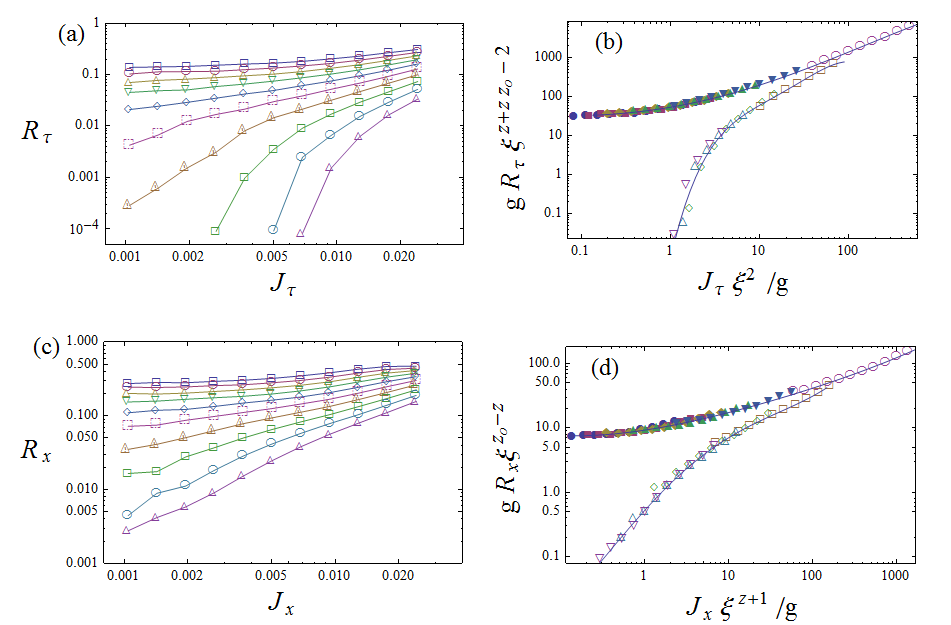
Figure 1: Scaling behavior of the phase slippage response for the gauge-glass model in (a) the imaginary-time direction $R_{\tau}$ and (c) spatial direction $R_{x}$ near the SI transition. From the top down, the couplings are $g=1.75,1.73,1.71,1.69,1.67,1.65,1.63,1.61,1.59$ and $1.57$. (b) and (d) Scaling plots corresponding to (a) and (c), respectively, for data near the transition with $\xi=|g/g_{c}-1|^{-\nu}$ using the same parameters $g_{c}=1.645$, $z_{o}=2.3$, $z=1.2$, and $\nu=0.9$.

To obtain the estimates above, it was implicitly assumed that he system is sufficient large and the coupling parameter is not too close to $g_{c}$, allowing the finite-size effects to be neglected. Having obtained an estimate of $z$, we can now consider the finite-size behavior of the phase stiffness in the imaginary time direction $\gamma_{\tau}$, using equilibrium MC simulations, and improve the determination of $g_{c}$ and $\nu$. The phase stiffness $\gamma_{\tau}$, which is a measure of the free energy cost to impose an infinitesimal phase twist in the time direction, is given by Cha and Girvin (1994)

$$\gamma_{\tau}=\frac{1}{L^{2}L_{\tau}g^{2}}[g<\epsilon_{\tau}>-<I_{\tau}^{2}>+<I_{\tau}>^{2}]_{D},$$ (7)

where $\epsilon_{\tau}=\sum_{\tau,i}\cos(\theta_{\tau,i}-\theta_{\tau+1,i})$ and $I_{\tau}=\sum_{\tau,i}\sin(\theta_{\tau,i}-\theta_{\tau+1,i})$. In Eq. (7), $<\ldots>$ represents a MC average for a fixed disorder configuration and $[\ldots]_{D}$ represents an average over different disorder configurations. In the superconducting phase $\gamma_{\tau}$ should be finite, reflecting the existence of phase coherence, while in the insulating phase it should vanish in the thermodynamic limit. For a continuous phase transition, $\gamma_{\tau}$ should satisfy the finite-size scaling form

$$\gamma_{\tau}L^{2-z}=F(L^{1/\nu}\delta g),$$ (8)

where $F(x)$ is a scaling function and $\delta g=g-g_{c}$. This scaling form implies that data for $\gamma_{\tau}L^{2-z}$ as a function of $g$, for different system sizes $L$, should cross at the critical coupling $g_{c}$. Fig. 2a shows this crossing behavior obtained near the initial estimate of $g_{c}$ obtained from Fig. 1. by varying slightly $g_{c}$ and $\nu$ from their initial values. In the Inset of this Figure, we show a scaling plot of the data according to the scaling form of Eq. 8, which provides for the gauge-glass model the final estimates $g_{c}=1.649$ and $\nu=0.99$. The same value of the dynamic exponent $z=1.2$ found for the gauge-glass model also give consistent results for the other models. Figures 3 and 4 show the scaling behavior of the phase stiffness for the flux and binary phase-glass model. We then obtain the estimates $g_{c}=1.629$ and $\nu=0.92$ (flux glass), $g_{c}=1.58$ and $\nu=1.15$ (binary phase glass), $g_{c}=1.44$ and $\nu=1.12$ (Gaussian phase glass).

The SI transition can be further characterized by the behavior of the finite-size correlation length, which can be defined as Ballesteros et al. (2000)

$$\xi(L,g)=\frac{1}{2\sin(k_{0}/2)}[S(0)/S(k_{0})-1]^{1/2}.$$ (9)

Here $S(k)$ is the Fourier transform of the correlation function $C(r)$ and $k_{0}$ is the smallest nonzero wave vector. For $g>g_{c}$, this definition corresponds to a finite-difference approximation to the infinite system correlation length $\xi^{(}g)^{2}=-\frac{1}{S(k)}\frac{\partial S(k)}{\partial k^{2}}|_{k=0}$, taking into account the lattice periodicity. For the random-gauge models considered here, it is convenient to define the correlation function in terms of the overlap order parameter Bhatt and Young (1988) $q_{\tau,j}=\exp(i(\theta^{1}_{\tau,j}-\theta^{2}_{\tau,j}))$, where $1$ and $2$ label two different copies of the system with the same coupling parameters. The correlation function in the spatial direction is obtained as

$$C(r)=\frac{1}{L^{2}L_{\tau}}\sum_{\tau,j}<q_{\tau,j}q_{\tau,j+r}>,$$ (10)

and the analogous expression is used for the correlation function $C_{\tau}(r)$ in the time direction. For a continuous transition, $\xi(L,g)$ should satisfy the scaling form

$$\xi/L=F(L^{1/\nu}\delta g),$$ (11)

where $F(x)$ is a scaling function. Figures 5 and 6 show the behavior of the correlation length $\xi_{\tau}$ and $\xi$ in the time and spatial directions, for the gauge-glass model. The curves for $\xi_{\tau}/L$ as a function of $g$ for different system sizes cross at the same point, providing further evidence of a continuous transition. In the inset of Fig. 5, a scaling plot according to Eq. (11) is shown, which gives an alternative estimate of $g_{c}=1.646$ and $\nu=1.08$. For the correlation length in the spatial direction shown in Fig. 6 and the corresponding scaling plot, we obtain $g_{c}=1.629$ and $\nu=1.12$. Since in this case the crossing point is less clear, these estimates are more affected by corrections to finite-size scaling. For the flux and phase-glass models the difference of the estimate of $g_{c}$ from the correlation in the time and spatial directions are much larger. We consider that the results obtained from the scaling of the phase stiffness $\gamma_{\tau}$ are more accurate and use them to obtain the final result and the associated errorbar.

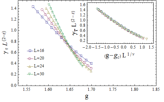
Figure 2: Phase stiffness in the imaginary time direction $\gamma_{\tau}$ for the gauge-glass model with different system sizes $L$, near the transition point estimated from Figs. 1. $L_{\tau}=aL^{z}$, with aspect ratio $a=0.642$ and $z=1.2$. Inset: scaling plot of $\gamma_{\tau}$ with $g_{c}=1.649$ and $\nu=0.99$. .

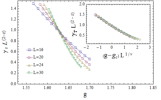
Figure 3: Same as Fig. 2 but for the flux-glass model. Inset: scaling plot of $\gamma_{\tau}$ with $g_{c}=1.6294$ and $\nu=0.92$ .

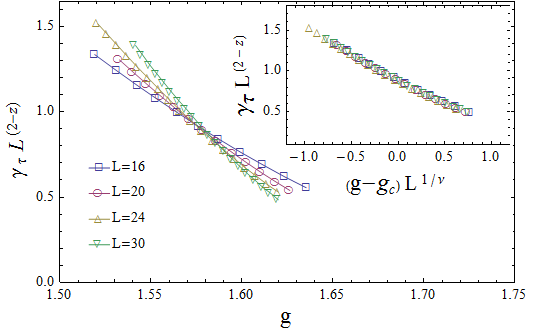
Figure 4: Same as Fig. 2 but for the phase-glass model. Inset: scaling plot of $\gamma_{\tau}$ with $g_{c}=1.58$ and $\nu=1.15$ .

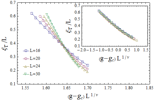
Figure 5: Correlation length in the imaginary time direction $\xi_{\tau}$ for the gauge-glass model with different system sizes $L$. Inset: scaling plot of $\xi_{\tau}$ with $g_{c}=1.646$ and $\nu=1.08$. .

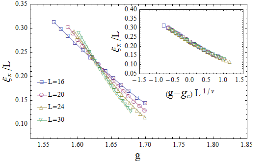
Figure 6: Correlation length in the spatial direction $\xi$ for the gauge-glass model with different system sizes $L$. Inset: scaling plot of $\xi$ with $g_{c}=1.629$ and $\nu=1.12$. .

We have also determined the universal conductivity at the critical point from the frequency and finite-size dependence of the phase stiffness $\gamma(w)$ in the spatial direction, following the scaling method described by Cha et al. Cha and Girvin (1994); Cha et al. (1991). The conductivity is given by the Kubo formula

$$\sigma=2\pi\sigma_{Q}\lim_{w_{n}\rightarrow 0}\frac{\gamma(iw_{n})}{w_{n}},$$ (12)

where $\sigma_{Q}=(2e)^{2}/h$ is the quantum of conductance and $\gamma(iw_{n})$ is a frequency dependent phase stiffness evaluated at the finite frequency $w_{n}=2\pi n/L_{\tau}$, with $n$ an integer. The frequency dependent phase stiffness in the $\hat{x}$ direction is given by

$$\gamma=\frac{1}{L^{2}L_{\tau}g^{2}}[ g <\epsilon_{x}>-<|I(iw_{n})|^{2}>$$ (13)

$$+ <|I(iw_{n})|>^{2}]_{D},$$ (14)

where

$$\epsilon_{x} = \sum_{\tau,j}e_{i,j+\hat{x}}\cos(\Delta_{x}\theta_{\tau,j}),$$ (15)

$$I(iw_{n}) = \sum_{\tau,j}e_{i,j+\hat{x}}\sin(\Delta_{x}\theta_{\tau,j})e^{iw_{n}\tau},$$ (16)

and $\Delta_{x}\theta_{\tau,j}=\theta_{\tau,j}-\theta_{\tau,j+\hat{x}}-A_{j,j+\hat{x}}$. At the transition, $\gamma(iw_{n})$ vanishes linearly with frequency and $\sigma$ assumes a universal value $\sigma^{*}$, which can be extracted from its frequency and finite-size dependence as Cha and Girvin (1994)

$$\frac{\sigma(iw_{n})}{\sigma_{Q}}=\frac{\sigma*}{\sigma_{Q}}-c(\frac{w_{n}}{2\pi}-\alpha\frac{2\pi}{w_{n}L_{\tau}})\cdots$$ (17)

The parameter $\alpha$ is determined from the best data collapse of the frequency dependent curves for different systems sizes in a plot of $\frac{\sigma(iw_{n})}{\sigma_{Q}}$ versus $x=(\frac{w_{n}}{2\pi}-\alpha\frac{2\pi}{w_{n}L_{\tau}})$. The universal conductivity is obtained from the intercept of these curves with the line $x=0$. The calculations were performed for different system sizes with $L_{\tau}=aL^{z}$, using the above estimates of $z$ and $g_{c}$. From the scaling behavior in Fig. 7 we obtain for the gauge-glass model $\sigma^{*}/\sigma_{Q}=0.56(3)$, where the estimated uncertainly is mainly the result of the error in the coupling $g_{c}$. Fig. 8 and Fig. 9 show the behavior for the flux and binary phase-glass models. We then obtain $\sigma^{*}/\sigma_{Q}=0.61(3)$ (flux glass), $\sigma^{*}/\sigma_{Q}=0.60(3)$ (binary phase glass) and $\sigma^{*}/\sigma_{Q}=0.57(3)$ (Gaussian phase glass)

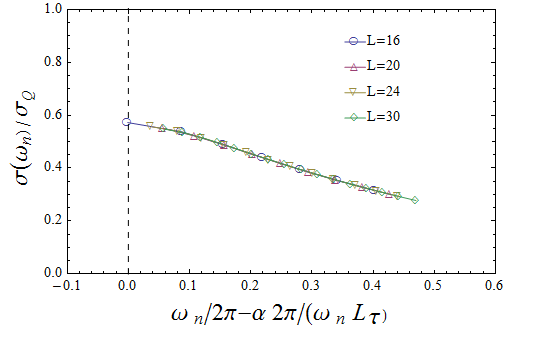
Figure 7: Scaling plot of conductivity $\sigma(iw_{n})$ at the critical coupling $g_{c}$ for the gauge-glass model with $\alpha=0.2$. The universal conductivity is given by the intercept with the $x=0$ dashed line, leading to $\frac{\sigma^{*}}{\sigma_{Q}}=0.56(3)$.

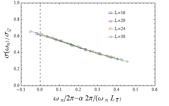
Figure 8: Same as Fig. 7 but for the flux-glass model with $\alpha=0.27$. The universal conductivity is given by the intercept with the $x=0$ dashed line, leading to $\frac{\sigma^{*}}{\sigma_{Q}}=0.61(3)$.

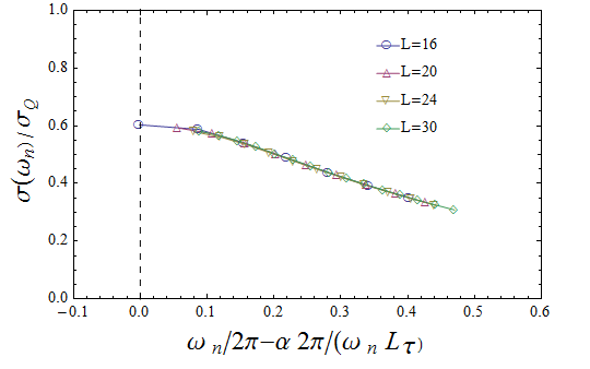
Figure 9: Same as Fig. 7 but for the binary phase-glass model with $\alpha=0.06$. The universal conductivity is given by the intercept with the $x=0$ dashed line, leading to $\frac{\sigma^{*}}{\sigma_{Q}}=0.60(3)$.

	pure	gauge	flux	binary	Gaussian
		glass	glass	phase glass	phase glass
$g_{c}$	$2.203$	$1.649(1)$	$1.629(1)$	$1.580(5)$	$1.440(5)$
$z$	$1$	$1.2(1)$	$1.2(1)$	$1.2(1)$	$1.2(1)$
$\nu$	$0.67$	$0.99(4)$	$0.92(4)$	$1.15(6)$	$1.12(4)$
$\sigma^{*}/\sigma_{Q}$	$0.29(2)$	$0.56(3)$	$0.61(3)$	$0.60(3)$	$0.57(3)$

Table 1: Critical exponents $z,\nu$ and critical conductivity $\sigma^{*}$ for different random gauge models and the pure model (without disorder). $g_{c}$ is the critical value of the coupling parameter $g=(E_{C}/E_{J})^{1/2}$. The results for the pure case are taken from ref. Cha et al., 1991.

The results for the critical properties of the different random gauge models are summarized in Table I, together with the known values for the pure model. We now compare them with available numerical work and experimental data. The value of the universal conductivity found in the earlier work on the gauge-glass model Kim and Stroud (2008), $\frac{\sigma^{*}}{\sigma_{Q}}=1.06(9)$, differs significantly from our result but the critical exponent $z=1.3(1)$ is consistent with our estimate. The discrepancy in the value of $\sigma^{*}$ is mainly due to the different estimate of the critical coupling, $g_{c}\approx 1.587$, which was obtained by a scaling analysis of the dimensionless ratio of the overlap order parameter $q_{\tau,j}$. This type of ”Binder ratio”, however, is not very reliable for models with continuous symmetry Shirakura and Matsubara (2003). Since our estimate of $g_{c}$ is based on the scaling behavior of the phase stiffness, which is also consistent with the behavior of the correlation length, we believe it should be more accurate. A different calculation of the critical exponents Tang and Chen (2008) found $\nu\approx 0.73$ and estimate $z=1.17(7)$, also compatible with our result for $z$.

The results for the gauge and flux-glass models can be compared with experimental observations of the SI transition on thin superconducting films with a pattern of nanoholes Stewart et al. (2007); Nguyen et al. (2015, 2016). A minimal model describing phase coherence in these systems consists of a Josephson-junction array defined on an appropriate lattice, with the nanoholes corresponding to the dual lattice Granato (2013, 2016b, 2016a). Very recently Nguyen et al. (2015, 2016), the effect of controlled amount of gauge disorder on the SI transition was investigated by introducing geometrical disorder in the form of randomness in the position of the nanoholes. This leads to disorder in the magnetic flux $\delta f_{p}=B\delta S_{p}/\Phi_{o}$ in a plaquette of area $S_{p}$, which increases with the applied magnetic field and degree of geometrical disorder. Magnetoresistance oscillations near the SI transition, resulting from commensurate vortex-lattice states, are observed below a critical disorder strength Nguyen et al. (2015) $\delta f_{c}\approx 0.3$. Although the resistivity at successive field-induced SI transitions varies below this critical disorder, it seems to reach a constant value, independent of the critical coupling for larger disorder Nguyen et al. (2016). Recent numerical simulations of a Josephson-junction array model suggests that the large disorder regime should correspond to a vortex glass Granato (2016a). The gauge and flux-glass models considered here should then provided the simplest description in this limit. For weak geometrical disorder, the nanoholes form a triangular lattice Stewart et al. (2007) and therefore the appropriate geometry for the array model should be a honeycomb lattice Granato (2016a, in press). In the large disorder limit, however, the lattice geometry should not be relevant. In fact, the numerical results for the conductivity at the transition found for a flux-glass model using a honeycomb lattice in the large disorder limit Granato (2016a) is the same, within the estimated errorbar, as found in the present work for the square lattice. In particular, the value of conductivity at the transition found in the experiments for large gauge disorder Nguyen et al. (2015, 2016) is a factor of $~{}2$ larger compared with measurements on samples without an applied magnetic field Stewart et al. (2007). This ratio of the critical conductivities agrees with the results for the gauge or flux-glass models compared with the pure model in Table I. Therefore, although the magnitudes of the experimental and numerical results are different, the trend of increasing critical conductivity with gauge disorder is correctly given by the gauge and flux-glass models. Notice, however, that the opposite trend can occur when comparing the large gauge disorder limit with the pure system in presence of a magnetic field Granato (2016a). Moreover, the agreement of the critical properties obtained from the gauge and flux-glass models and the previous calculations for large disorder from a model on a honeycomb lattice Granato (2016a), strongly supports the experimental observation Nguyen et al. (2016) that the critical conductivity is independent of the coupling parameter in the large disorder limit.

It may appear somehow surprising that the critical conductivity for the phase-glass model is essentially the same as for the gauge-glass model. The phase-glass model has an additional reflection symmetry property Kawamura (1995), where changing $\theta_{i}\rightarrow-\theta_{i}$ leaves the Hamiltonian unchanged, whereas for the gauge-glass model there is only a continuous symmetry. One could then expect different universality classes. In the absence of quantum fluctuations, $E_{c}=0$, this happens to be the case. In 2D, the transition for increasing temperatures can be described as a thermal transition with vanishing critical temperature, $T_{c}=0$, and a divergent thermal correlation length $\xi_{T}\propto T^{-\nu_{T}}$. In fact, the value of $\nu_{T}$ for the gauge and phase-glass models are quite different Kawamura and Tanemura (1991); Granato (1998). On the other hand, the SI transition at zero temperature is actually described by an effective $(2+1)$D classical model (Eq. (3)) with gauge disorder completely correlated in one direction. Interestingly, numerical results for the 3D gauge and phase-glass models show the same critical exponents Wengel and Young (1997); Granato (2004); Lee and Young (2003), within the estimated errorbar, although such calculations have only been carried out for models with uncorrelated disorder.

IV Conclusions

We studied the superconductor-insulator transition in two-dimensional inhomogeneous superconductors with gauge disorder, described by four different models: a gauge glass, a flux glass, a binary phase glass and Gaussian phase-glass model. The first two models, describe the combined effect of geometrical disorder in the array of local superconducting islands and a uniform external magnetic field while the last two describe the effects of randomness in the Josephson couplings alone, allowing for negative couplings. We found that the gauge and flux-glass models display the same critical behavior, within the estimated uncertainties, and similar behavior is observed for binary and Gaussian phase-glass models. The value of the conductivity at the transition is a factor of 2 larger than for the pure model, which agrees with recent experiments on nanohole thin film superconductors Nguyen et al. (2015, 2016) in the large disorder limit, which can be modeled by the gauge or flux-glass models. This agreement together with previous results for large disorder from a model on a honeycomb lattice Granato (2016a), strongly supports the experimental observation Nguyen et al. (2016) that the critical conductivity is independent of the coupling parameter in the large disorder limit, consistent with the scenario of a universal value in this limit. For a more realistic description of these systems dissipation effects Fazio and van der Zant (2001), which have been neglected in the present models, should also be taken into account. It should be noted that the phase-glass models considered here, which show a direct superconductor to insulator transition, have a zero mean distribution of Josephson couplings. For a nonzero mean, an analytical work Phiillips (2003) has proposed an intermediate metallic phase (a Bose metal) separating the superconducting and insulating phases.