Asymptotic and finite-time almost global attitude tracking: representations free approach

Abstract

In this paper, the attitude tracking problem is considered using the rotation matrices. Due to the inherent topological restriction, it is impossible to achieve global attractivity with any continuous attitude control system on $SO(3)$. Hence in this work, we propose some control protocols achieve almost global tracking asymptotically and in finite time, respectively. In these protocols, no world frame is needed and only relative state informations are requested. For finite-time tracking case, Filippov solutions and non-smooth analysis techniques are adopted to handle the discontinuities. Simulation examples are provided to verify the performances of the control protocols designed in this paper.

I Introduction

Originally motivated by aerospace developments in the middle of the last century [4, 15], the rigid body attitude control problem has continued to attract attention with many applications such as aircraft attitude control [1, 31], spacial grabbing technology of manipulators [21], target surveillance by unmanned vehicles [24], and camera calibration in computer vision [20]. Furthermore, the configuration space of rigid-body attitudes is the compact non-Euclidean manifold $SO(3)$, which poses theoretical challenges for attitude control [2]. The coordination of multiple attitudes is of high interest both in academic and industrial research, e.g., [9, 26, 28].

Here we review some related existing work. As attitude systems evolves on $SO(3)$—a compact manifold without a boundary—there exists no continuous control law that achieves global asymptotic stability [5]. Hence one has to resort to some hybrid or discontinuous approaches. In [16], exponential stability is guaranteed for the tracking problem for a single attitude. In [19] the authors considered the synchronization problem of attitudes under a leader-follower architecture. In [23], the authors provided a local result on attitude synchronization. Based on a passivity approach, [25] proposed a consensus control protocol for multiple rigid bodies with attitudes represented by modified Rodrigues parameters. In [30], the authors provided a control protocol in discrete time that achieves almost global synchronization, but it requires global knowledge of the graph topology. Although there exists no continuous control law that achieves global asymptotic stability, a methodology based on the axis-angle representation obtains almost global stability for attitude synchronization under directed and switching interconnection topologies is proposed in [29].

Besides these agreement results, some tracking results are reviewed as follows. In [18], an almost global attitude tracking control system based on an alternative attitude error function is proposed. This attitude error function is not differentiable at certain attitudes and employs the Frobenius attitude difference, and the resulting control input is not continuous. In [17], one tracking protocol is proposed for unmanned aerial vehicle (UAV), again using Frobenius state differences. So far, finite-time attitude tracking problems are studied in different settings, e.g., [10, 32]. In [10], finite-time attitude synchronization was investigated in a leader-follower architecture, namely all the followers tracking the attitude of the leader. In [32], quaternion representation was employed for finite-time attitude synchronization. Both works used continuous control protocols with high-gain.

In this paper, we shall focus on the attitude tracking problem, based on the rotation matrices in $SO(3)$. The contributions are threefolds. First, based on the two types of relative state difference, geodesic or Frobenius, two types of control schemes are proposed. Let us refer these two type of protocols as geodesic and Frobenius controller, respectively. In both types of the controllers, only the relative state informations, with no world frame, are needed. Second, for both geodesic and Frobenius controllers, we propose one for asymptotic tracking and one for finite-time tracking. More precisely, sign function is employed for the finite-time case. Since these control schemes are discontinuous, nonsmooth analysis is employed throughout the paper. Third, all the controllers designed in this paper achieves almost global tracking.

The structure of the paper is as follows. In Section II, we review some results for the special orthogonal group $SO(3)$ and introduce some terminologies and notations in the context of discontinuous dynamical systems. Section III presents the problem formulation of the attitude tracking. The main results of the stability analysis of the finite-time convergence are presented in Section IV, where two types of controllers, using geodesic and Frobenius state differences, respectively, are proposed to achieve almost global tracking. The simulations of the main results are in Section V. Then, in Section VI, the paper is concluded.

Notations. With $\mathbb{R}_{-},\mathbb{R}_{+},\mathbb{R}_{\geqslant 0}$ and $\mathbb{R}_{\leqslant 0}$ we denote the sets of negative, positive, non-negative, non-positive real numbers, respectively. The rotation group $SO(3)=\{R\in\mathbb{R}^{3\times 3}:RR^{\top}=I,\det R=1\}.$ The vector space of real $n$ by $n$ skew symmetric matrices is denoted as $\mathfrak{so}(3)$. The vectors $\mathds{1}_{n}$ and $\mathbf{0}_{n}$ represents a $n$-dimensional column vector with each entry being $1$ and $0$, respectively. We denote

$$E_{1} =\operatorname{diag}{[-1,-1,1]}$$

$$E_{2} =\operatorname{diag}{[-1,1,-1]}$$

$$E_{3} =\operatorname{diag}{[1,-1,-1]},$$

respectively.

II Preliminaries

In this section, we briefly review some essentials about rigid body attitudes [27], and give some definitions for Filippov solutions [11].

Next lemma follows from Euler’s Rotation Theorem.

Lemma 1.

The exponential map

$$\exp:\mathfrak{so}(3)\rightarrow SO(3)$$ (1)

is surjective.

The tangent space at a point $R\in SO(3)$ is

$$T_{R}SO(3)=\{R\omega:\omega\in\mathfrak{so}(3)\}.$$ (2)

For $SO(3)$, two exponential maps are needed, namely Riemannian exponential at the point $R$ and Lie group exponential, denoted $\exp_{R}$ and $\exp$ respectively.

For any $p=[p_{1},p_{2},p_{3}]^{\top}\in\mathbb{R}^{3}$ and $\hat{p}\in\mathfrak{so}(3)$ given as

$$\hat{p}:=\begin{pmatrix}0&-p_{3}&p_{2}\\ p_{3}&0&-p_{1}\\ -p_{2}&p_{1}&0\end{pmatrix},$$ (3)

Rodrigues’ formula is the right-hand side of

$$\exp(\hat{p})=\begin{cases}I_{3}+\frac{\sin(\|p\|)}{\|p\|}\hat{p}+\frac{1-\cos(\|p\|)}{\|p\|^{2}}(\hat{p})^{2},&\textrm{ if }\|p\|\neq 0,\\ I_{3},&\textrm{ if }\|p\|=0.\end{cases}$$ (4)

The matrix $\exp(\hat{p})$ is the rotation matrix through an angle $\|p\|$ anticlockwise about the axis $p$. The Riemannian exponential map $\exp_{R}:T_{R}SO(3)\rightarrow SO(3)$ is defined as

$$\exp_{R_{1}}(v)=\gamma(1)$$ (5)

where

$$\gamma(t)=R_{1}(R_{1}^{\top}R_{2})t,\quad 0\leqslant t\leqslant 1$$ (6)

is the length of the shortest geodesic curve that connect $R_{1}$ and $R_{2}$, and $\gamma^{\prime}(0)=v$. The relation between these exponential maps is $\exp_{R}(RW)=R\exp(W)$ for any $RW\in T_{R}SO(3)$.

The principle logarithm for a matrix $R\in SO(3)$ is defined as

$$\log(R)=\begin{cases}\frac{\theta}{2\sin(\theta)}(R-R^{\top}),&\textrm{ if }\theta\neq 0,\\ \mathbf{0},&\textrm{ if }\theta=0\end{cases}$$ (7)

where $\theta=\arccos(\frac{\operatorname{tr}(R)-1}{2})$. We define $\log(I_{3})$ as the zero matrix in $\mathbb{R}^{3\times 3}$. Note that (7) is not defined for $\theta=\pi$.

There are three commonly used metrics in $SO(3)$. A straightforward one is Frobenius (chordal) metric

$$d_{F}(R_{1},R_{2}) =\|R_{1}-R_{2}\|_{F}$$ (8)

$$=\sqrt{6-\operatorname{tr}(R^{\top}_{1}R_{2})-\operatorname{tr}(R^{\top}_{2}R_{1})},$$ (9)

which is Euclidean distance of the ambient space $\mathbb{R}^{3\times 3}$. Another metric employs the Riemannian structure, namely the Riemannian (geodesic) metric

$$d_{R}(R_{1},R_{2})=\frac{1}{\sqrt{2}}\|\log(R^{-1}_{1}R_{2})\|_{F}.$$ (10)

The third one is hyperbolic metric defined as $d_{H}(R_{1},R_{2})=\|\log(R_{1})-\log(R_{2})\|_{F}$.

One important relation between $SO(3)$ and $\mathbb{R}^{3}$ is that the open ball $B_{\pi}(I)$ in $SO(3)$ with radius $\pi$ around the identity, which is almost the whole $SO(3)$, is diffeomorphic to the open ball $B_{\pi}(0)$ in $\mathbb{R}^{3}$ via the logarithmic and the exponential map defined in (7) and (4).

In the remainder of this section, we discuss Filippov solutions [12]. Consider the system

$$\dot{x}=f(x,t)$$ (11)

where $x(t)\in\mathcal{D}\subset\mathbb{R}^{n}$ denotes the state vector, $f:\mathcal{D}\times[0,\infty)\rightarrow\mathbb{R}^{n}$ is Lebesgue measurable and essentially locally bounded, uniformly in $t$ and $\mathcal{D}$ is an open and connected set.

Definition 1 (Filippov solution [11, 12]).

A function $x:[0,\infty)\rightarrow\mathbb{R}^{n}$ is called a solution of (11) on the interval $[0,\infty)$ if $x(t)$ is absolutely continuous and for almost all $t\in[0,\infty)$

$$\dot{x}\in\mathcal{F}[f](x(t),t)$$ (12)

where $\mathcal{F}[f](x(t),t)$ is an upper semi-continuous, nonempty, compact and convex valued map on $\mathcal{D}$, defined as

$$\mathcal{F}[f](x(t),t):=\bigcap_{\delta>0}\bigcap_{\mu(S)=0}\overline{\mathrm{co}}\big{\{}f(B(x,\delta)\backslash S,t)\big{\}},$$ (13)

where $S$ is a subset of $\mathbb{R}^{n}$, $\mu$ denotes the Lebesgue measure, $B(x,\delta)$ is the ball centered at $x$ with radius $\delta$ and $\overline{\mathrm{co}}\{\mathcal{X}\}$ denotes the convex closure of a set $\mathcal{X}$.

If ${f}$ is continuous at $x$, then $\mathcal{F}[{f}](x)$ contains only the point ${f}(x)$.

A Filippov solution is maximal if it cannot be extended forward in time, that is, if it is not the result of the truncation of another solution with a larger interval of definition. Next, we introduce invariant sets, which will play a key part further on. Since Filippov solutions are not necessarily unique, we need to specify two types of invariant sets. A set $\mathcal{R}\subset\mathbb{R}^{n}$ is called weakly invariant if, for each $x_{0}\in\mathcal{R}$, at least one maximal solution of (12) with initial condition $x_{0}$ is contained in $\mathcal{R}$. Similarly, $\mathcal{R}\subset\mathbb{R}^{n}$ is called strongly invariant if, for each $x_{0}\in\mathcal{R}$, every maximal solution of (12) with initial condition $x_{0}$ is contained in $\mathcal{R}$. For more details, see [8, 11]. We use the same definition of regular function as in [7] and recall that any convex function is regular. And any $\mathcal{C}^{1}$ continuous function is regular.

For $V:\mathbb{R}^{n}\times[0,\infty)\rightarrow\mathbb{R}$ locally Lipschitz in $(x,t)$, the generalized gradient $\partial V$ is defined by

$$\partial V(x,t):= \mathrm{co}\Big{\{}\lim_{i\rightarrow\infty}\nabla V(x_{i},t_{i})\mid(x_{i},t_{i})\rightarrow(x,t),$$

$$(x_{i},t_{i})\notin S\cup\Omega_{{f}}\Big{\}},$$

where $\nabla$ is the gradient operator, $\Omega_{{f}}\subset\mathbb{R}^{n}\times[0,\infty)$ is the set of points where $V$ fails to be differentiable and $S\subset\mathbb{R}^{n}\times[0,\infty)$ is a set of measure zero that can be arbitrarily chosen to simplify the computation, since the resulting set $\partial V(x,t)$ is independent of the choice of $S$ [7].

Given a set-valued map $\mathcal{T}:\mathbb{R}^{n}\times[0,\infty)\rightarrow 2^{\mathbb{R}^{n}}$, the set-valued Lie derivative $\mathcal{L}_{\mathcal{T}}V$ of a locally Lipschitz function $V:\mathbb{R}^{n}\times[0,\infty)\rightarrow\mathbb{R}$ with respect to $\mathcal{T}$ at $(x,t)$ is defined as

$$\mathcal{L}_{\mathcal{T}}V(x,t):= \big{\{}a\in\mathbb{R}\mid\exists\nu\in\mathcal{T}(x)\textnormal{ such that }$$ (14)

$$\quad\zeta^{T}\begin{bmatrix}\nu\\ 1\end{bmatrix}=a,\,\forall\zeta\in\partial V(x,t)\big{\}}.$$

III Problem formulation

In this paper we consider attitude tracking problem. The basic model can be considered as two agent network where the follower tracks the attitude of the target. We denote the world frame as $\mathcal{F}_{w}$, the instantaneous body frame of the target and the follower as $\mathcal{F}_{r}$ and $\mathcal{F}_{1}$, respectively. Let $R_{r}(t),R_{1}(t)\in SO(3)$ be the attitude of $\mathcal{F}_{r}$ and $\mathcal{F}_{1}$ relative to $\mathcal{F}_{w}$ at time $t$.

Recall that the tangent space at a point $R\in SO(3)$ is

$$T_{R}SO(3)=\{R\omega:\omega\in\mathfrak{so}(3)\}.$$ (15)

Then the kinematics of the two attitudes are given by [27]

$$\dot{R}=\operatorname{diag}(R_{r},R_{1})\omega$$ (16)

where

$$R =[R^{\top}_{r},R^{\top}_{1}]^{\top},$$ (17)

$$\omega =[\omega^{\top}_{r},\omega^{\top}_{1}]^{\top},$$

where $\omega_{1}$ is the control input to design

By asymptotic and finite time attitude tracking we mean that for the multi-agent system (16), the absolute rotations of agent 1 track the rotation of the target in the world frame $\mathcal{F}_{w}$ asymptotically and in finite time, respectively. In other words,

$$R_{1}\rightarrow R_{r},\textnormal{ as }t\rightarrow\infty,\textnormal{ and }$$

$$\exists T>0,\textnormal{ s.t. } R_{1}\rightarrow R_{r},\textnormal{ as }t\rightarrow T,$$

respectively.

IV Main result: single agent tracking

In this section, we first assume that the desired velocity $\omega_{r}(t)\in\mathfrak{so}(3)$ and the geodesic difference are available to the agent 1. Here we present two controllers as

$$\omega_{1,a} =\log(R^{-1}_{1}R_{r})+\omega_{r},$$ (18)

$$\omega_{1,f} =\frac{1}{\|\log(R^{-1}_{1}R_{r})\|_{F}}\log(R^{-1}_{1}R_{r})+\omega_{r},$$ (19)

which will be proved to achieve asymptotic and finite-time tracking, respectively.

As discontinuities are introduced if the controller (19) is employed, we shall understand the trajectories in the sense of Filippov, namely an absolutely continuous function $x(t)$ satisfying the differential inclusion

$$\begin{bmatrix}\dot{R}_{r}\\ \dot{R}_{1}\end{bmatrix} \in\begin{bmatrix}R_{r}\omega_{r}\\ \mathcal{F}[R_{1}\omega_{1,f}]\end{bmatrix}$$ (20)

$$=:\mathcal{F}_{1}$$

for almost all time, where we used Theorem 1(5) in [22].

Theorem 2.

Consider system (16). Assume the system initialized without singularity, i.e., $\arccos(\frac{\operatorname{tr}(R^{\top}_{r}(0)R_{1}(0))-1}{2})\neq\pi$. Then

1. the singularity is avoided for all time for both controller (18) and (19);

2. the attitude $R_{1}$ tracks $R_{r}$ exponentially and in finite time, respectively, by (18) and (19). For (19), the conclusion holds for all the solutions.

Proof.

The proof is divided into two parts, one for each controller (18) and (19).

Part I: In this part, we prove that by using controller (18), the asymptotic tracking is achieved and the singularity is avoided. We can write the closed-loop as

$$\dot{R}_{r} =R_{r}\omega_{r}$$

$$\dot{R}_{1} =R_{1}(\log(R^{-1}_{1}R_{r})+\omega_{r})$$

Notice that the singularity only happens at $\theta=\arccos(\frac{\operatorname{tr}(R^{\top}_{r}R_{1})-1}{2})=\pi$, hence we only need to show that $\theta(t)\in[0,\pi)$ for all $t\geqslant 0$. Notice that

$$\frac{\partial\theta}{\partial R_{r}} =\frac{-1}{\sqrt{1-\Delta^{2}}}\frac{\partial\Delta}{\partial R_{r}}=\frac{-1}{2\sqrt{1-\Delta^{2}}}R_{1},$$ (21)

$$\frac{\partial\theta}{\partial R_{1}} =\frac{-1}{\sqrt{1-\Delta^{2}}}\frac{\partial\Delta}{\partial R_{1}}=\frac{-1}{2\sqrt{1-\Delta^{2}}}R_{r},$$

where $\Delta=\frac{\operatorname{tr}(R^{\top}_{1}R_{r})-1}{2}$. Then we have

$$\dot{\theta}(t)= \operatorname{tr}(\frac{\partial^{\top}\theta}{\partial R_{r}}\dot{R}_{r}+\frac{\partial^{\top}\theta}{\partial R_{1}}\dot{R}_{1})$$ (22)

$$= \frac{-1}{2\sqrt{1-\Delta^{2}}}\operatorname{tr}\Big{(}R^{\top}_{1}R_{r}\omega_{r}+R^{\top}_{r}R_{1}\omega_{r}$$ (23)

$$R^{\top}_{r}R_{1}\log(R^{\top}_{1}R_{r})\Big{)}$$ (24)

$$= \frac{-1}{2\sqrt{1-\Delta^{2}}}\operatorname{tr}\Big{(}R^{\top}_{r}R_{1}\log(R^{\top}_{1}R_{r})\Big{)}$$ (25)

$$= \frac{-1}{2\sqrt{1-\Delta^{2}}}\frac{\theta}{\sin(\theta)}\operatorname{tr}\Big{(}I-R^{\top}_{r}R_{1}R^{\top}_{r}R_{1}\Big{)}$$ (26)

$$\leqslant 0$$ (27)

where the last inequality is based on the fact that $R^{\top}_{r}R_{1}R^{\top}_{r}R_{1}\in SO(3)$. This proves that if the singularity is avoid at the initialization, then it is avoided along the trajectory.

Then consider the Lyapunov function $W(R_{r},R_{1})=d_{R}^{2}(R_{r},R_{1})=\frac{1}{2}\|\log(R^{\top}_{r}R_{1})\|_{F}^{2}$, and we have

$$\frac{\partial W}{\partial R_{r}} =-R_{r}\log(R^{\top}_{r}R_{1})$$ (28)

$$\frac{\partial W}{\partial R_{1}} =-R_{1}\log(R^{\top}_{1}R_{r})$$ (29)

and

$$\dot{W}(t)= \operatorname{tr}(\frac{\partial^{\top}W}{\partial R_{r}}\dot{R}_{r}+\frac{\partial^{\top}W}{\partial R_{1}}\dot{R}_{1})$$

$$= -\operatorname{tr}(\log^{\top}(R^{\top}_{1}R_{r})\log(R^{\top}_{1}R_{r}))$$

$$+\operatorname{tr}\Big{(}\log^{\top}(R^{\top}_{r}R_{1})\omega_{r}+\log^{\top}(R^{\top}_{1}R_{r})\omega_{r}\Big{)}$$

$$= -\operatorname{tr}\Big{(}\log^{\top}(R^{\top}_{1}R_{r})\log(R^{\top}_{1}R_{r})\Big{)}$$

$$= -2W.$$

Hence by LaSalle-Yoshizawa Theorem (see e.g., [6]), the follower tracks the attitude of the target exponentially.

Part II: In this part we prove that the finite-time tracking can be achieved by controller (19) and the singularity is avoided. The proof is similar to Part I. Hence we only provide the sketch.

For this case, we need to consider differential inclusion (20) since the discontinuity is present. Notice that the function $W$ and $\theta$ is $\mathcal{C}^{1}$, hence regular. Then for $\theta\neq 0$, i.e., $R^{\top}_{1}R_{r}\neq I$, we have

$$\mathcal{L}_{\mathcal{F}_{1}}\theta= \big{\{}\frac{-1}{2\sqrt{1-\Delta^{2}}}\frac{\theta}{\sin(\theta)}\frac{1}{\|\log(R^{\top}_{1}R_{r})\|_{F}}$$

$$\operatorname{tr}\Big{(}I-R^{\top}_{r}R_{1}R^{\top}_{r}R_{1}\Big{)}\big{\}}$$

$$\subset \mathbb{R}_{-}.$$

By the fact that $\theta$ is $\mathcal{C}^{1}$ continuous, hence $\theta(R_{r}(t),R_{1}(t))$ is absolutely continuous and $\dot{\theta}(t)$ exists almost everywhere which belongs to $\mathcal{L}_{\mathcal{F}_{1}}\theta$. Then

$$\theta(t)=\int_{0}^{t}\dot{\theta}(\tau)d\tau+\theta(0)\leqslant\theta(0),$$ (30)

which indicate the singularity is avoided.

Next, we prove the finite-time tracking. Consider the error $V:=W^{\alpha}$ with $\alpha>\frac{1}{2}$. Then the set-valued derivative is given as

$$\mathcal{L}_{\mathcal{F}_{1}}V=\begin{cases}\{-\alpha\sqrt{2}V^{\beta}\},&\textrm{ if }R_{1}^{\top}R_{r}\neq I\\ \{0\},&\textrm{ if }R_{1}^{\top}R_{r}=I\end{cases}$$

where $\beta=\frac{2\alpha-1}{2\alpha}\in(0,1)$. Notice that

$$\{(R_{r},R_{1})\mid 0\in\mathcal{L}_{\mathcal{F}_{1}}V\}=\{(R_{r},R_{1})\mid V=0\},$$ (31)

and $\dot{V}$ exists when $V\neq 0$, and $\dot{V}$ exists almost everywhere when $V=0$ (by the fact that $V$ is $\mathcal{C}^{1}$, hence regular) and $\dot{V}\subset\mathcal{L}_{\mathcal{F}_{1}}V=\{0\}$. In other words, we have

$$\dot{V}=-\alpha\sqrt{2}V^{\beta},\textnormal{ for }V\neq 0$$ (32)

with $\beta\in(0,1)$, which implies that $V$ converge to the origin in finite time (see, e.g., [14, 13]). Hence we the follower tracks the attitude of the target in finite time.

∎

In the controller (18) and (19), it is assumed that the geodesic state difference is available. In the rest part of this section, we show that the same conclusion as in Theorem 2 can be derived for the controller with Frobenius difference, which is relative information as well, i.e.,

$$\omega_{1,a} =R^{\top}_{1}R_{r}-R^{\top}_{r}R_{1}+\omega_{r},$$ (33)

$$\omega_{1,f} =\frac{1}{\|R_{1}-R_{r}\|_{F}}\big{(}R^{\top}_{1}R_{r}-R^{\top}_{r}R_{1}\big{)}+\omega_{r},.$$ (34)

Corollary 3.

Consider system (16). Assume the system initialized without singularity, i.e., $\arccos(\frac{\operatorname{tr}(R^{\top}_{r}(0)R_{1}(0))-1}{2})\neq\pi$. Then

1. the singularity is avoided for all time for both controller (33) and (34);

2. the attitude $R_{1}$ tracks $R_{r}$ exponentially and in finite time, respectively, by (33) and (34). For (34), the conclusion holds for all the solutions.

Proof.

Here the proof is similar to the one of Theorem 2, hence we only provide the sketch. Here the proof is again divided into two parts.

Part I: First, by (21), we have

$$\dot{\theta}(t)= \operatorname{tr}(\frac{\partial^{\top}\theta}{\partial R_{r}}\dot{R}_{r}+\frac{\partial^{\top}\theta}{\partial R_{1}}\dot{R}_{1})$$ (35)

$$= \frac{-1}{2\sqrt{1-\Delta^{2}}}\operatorname{tr}\Big{(}R^{\top}_{1}R_{r}\omega_{r}+R^{\top}_{r}R_{1}\omega_{r}$$ (36)

$$R^{\top}_{r}R_{1}(R^{\top}_{1}R_{r}-R^{\top}_{r}R_{1})\Big{)}$$ (37)

$$= \frac{-1}{2\sqrt{1-\Delta^{2}}}\operatorname{tr}\Big{(}R^{\top}_{r}R_{1}(R^{\top}_{1}R_{r}-R^{\top}_{r}R_{1})\Big{)}$$ (38)

$$= \frac{-1}{2\sqrt{1-\Delta^{2}}}\operatorname{tr}\Big{(}I-R^{\top}_{r}R_{1}R^{\top}_{r}R_{1}\Big{)}$$ (39)

$$\leqslant 0.$$ (40)

Hence the singularities are avoided along the trajectory, i.e., the rotation matrices $R_{r}(t)^{\top}R_{1}(t)\neq E_{i},i=1,2,3$ if the equality does not hold for $R_{r}(0)^{\top}R_{1}(0)$.

Then consider the Lyapunov function $W(R_{r},R_{1})=\frac{1}{2}d_{F}^{2}(R_{r},R_{1})=3-\operatorname{tr}{R^{\top}_{r}R_{1}}$, then

$$\dot{W}(t)= -\operatorname{tr}(R^{\top}_{r}\dot{R}_{1}+\dot{R}^{\top}_{r}R_{1})$$

$$= -\operatorname{tr}(R^{\top}_{r}R_{1}\omega_{r}+\omega^{\top}_{r}R^{\top}_{r}R_{1})$$

$$-\operatorname{tr}\Big{(}R^{\top}_{r}R_{1}(R^{\top}_{1}R_{r}-R^{\top}_{r}R_{1})\Big{)}$$

$$= -\operatorname{tr}\Big{(}I-R^{\top}_{r}R_{1}R^{\top}_{r}R_{1}\Big{)}$$

$$\leqslant 0.$$

Hence by LaSalle-Yoshizawa Theorem (see e.g., [6]), the follower tracks the attitude of the target asymptotically. Moreover, as the $\theta\rightarrow 0$ asymptotically, there exists $T$ such that for any $t\geqslant T$, we have

$$\operatorname{tr}(R^{\top}_{r}R_{1}R^{\top}_{r}R_{1})\leqslant\operatorname{tr}{R^{\top}_{r}R_{1}}.$$ (41)

Hence for $t\leqslant T$, $\dot{W}\leqslant-W$. This implies the convergence is in fact exponential.

Part II: The conclusion for controller (34) can be derived similar to the proof of Theorem 2, by using the Lyapunov function $V=W^{\alpha}$ for $\alpha\in(\frac{1}{2},\infty)$. ∎

Remark 1.

For the finite-time tracking controller (19) and (34), one closely related work is [10]. Compare the result here to the one in Section III in [10], which assumes that the absolute attitude, the bounded velocity, the bounded acceleration of the target are available to the follower, the advantages of our controllers are that the control laws are very intuitive, that we do not assume that the desired velocity is bounded, and that only relative measurement is needed, i.e., the geodesic and Frobenius difference.

V Simulations

In this section, we consider a specific trajectory of the target $R_{r}$ which is governed by

$$\dot{R}_{r}=R_{r}\omega_{r}$$

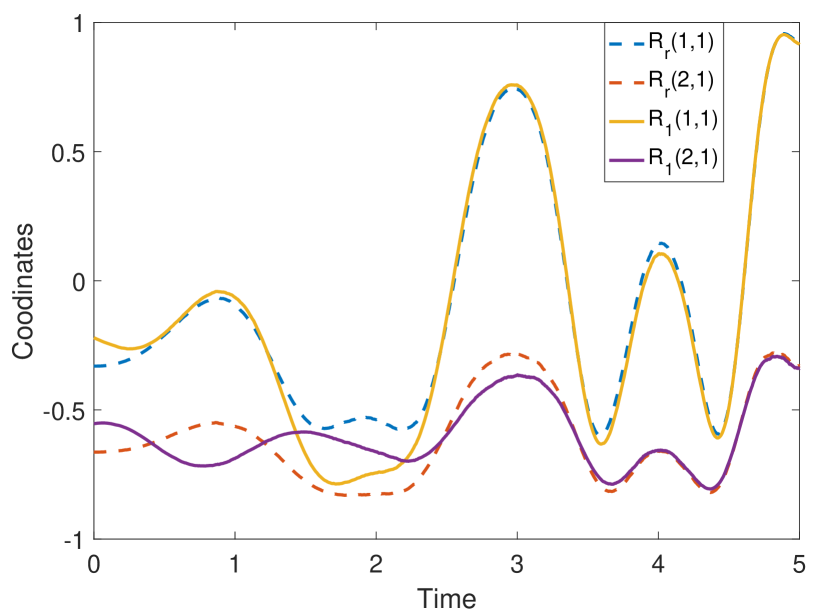
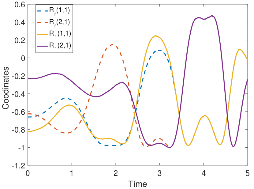
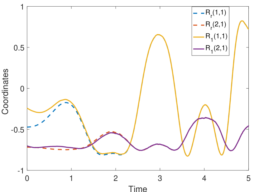
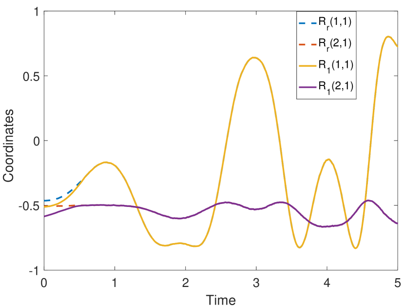
where $\omega^{\vee}_{r}(t)=t\sin(3\mathds{1}_{3}t)$. Notice that the reference velocity $\omega^{\vee}_{r}(t)$ is unbounded which is more general than the assumption in [10]. Here we present the simulation results of the control protocols (18),(19),(33) and (34), respectively. To make the graphical results more compact, we only show the trajectories of $R_{r}(i,1)$ and $R_{1}(i,1)$ for $i=1,2$, respectively. All the dynamical systems are initialized randomly without singularities.

For the case when geodesic differences are available, the results are shown in Fig.1. The dashed line is the trajectories of the target $R_{r}$ and the solid ones are of the follower. Asymptotic and finite-time tracking are depicted in Fig.1(a) and Fig.1(b), using controller (18) and (19), respectively. The similar results for (33) and (34) are shown in Fig.2.

(a) Evolution of the coordinates of $R_{r}(i,1),R_{1}(i,1),i=1,2$ of the system controlled by (18).

(b) Evolution of the coordinates of $R_{r}(i,1),R_{1}(i,1),i=1,2$ of the system controlled by (19). Finite-time consensus is achieved.

Figure 1: The simulation using geodesic difference.

(a) Evolution of the coordinates of $R_{r}(i,1),R_{1}(i,1),i=1,2$ of the system controlled by (33).

(b) Evolution of the coordinates of $R_{r}(i,1),R_{1}(i,1),i=1,2$ of the system controlled by (34). Finite-time consensus is achieved.

Figure 2: The simulation using Frobenius difference.

VI Conclusion

In this paper, we consider the asymptotic and finite-time attitude tracking problem. Based on the geodesic state difference, one asymptotic and finite-time tracking protocols are proposed. These protocols stabilize the system almost globally, i.e., the state of the follower tracks the attitude of the target if the system is initialized without singularity. For the finite-time controller, the solution of the closed-loop system is understood in the sense of Filippov. Similar protocols, asymptotic and finite-time one, are proposed if the Frobenius state differences are available. Future topics include estimation of the reference velocity using internal model principle, and tracking protocols using adaptive control mechanisms e.g.,prescribed performance control.

References

- [1] N. Athanasopoulos, M. Lazar, C. Böhm, and F. Allgöwer. On stability and stabilization of periodic discrete-time systems with an application to satellite attitude control. Automatica, 50(12):3190–3196, 2014.
- [2] S. Bhat and D. Bernstein. A topological obstruction to continuous global stabilization of rotational motion and the unwinding phenomenon. Systems & Control Letters, 39(1):63–70, 2000.
- [3] B. Bollobas. Modern Graph Theory, volume 184 of Graduate Texts in Mathematics. Springer, New York, 1998.
- [4] J. Bower and G. Podraza. Digital implementation of time-optimal attitude control. IEEE Transactions on Automatic Control, 9(4):590–591, 1964.
- [5] R. W. Brockett. Asymptotic stability and feedback stabilization. In Differential Geometric Control Theory (R. W. Brockett, R. S. Millman and H. J. Sussmann, Eds), pages 181–191. Birkhauser, Boston, 1983.
- [6] Z. Chen and J. Huang. Stabilization and Regulation of Nonlinear Systems: A Robust and Adaptive Approach. Advanced Textbooks in Control and Signal Processing. Springer International Publishing, 2015.
- [7] F. H. Clarke. Optimization and Nonsmooth Analysis. Classics in Applied Mathematics. Society for Industrial and Applied Mathematics, 1990.
- [8] J. Cortés. Discontinuous dynamical systems. Control Systems, IEEE, 28(3):36–73, 2008.
- [9] Y. Dong and Y. Ohta. Attitude synchronization of rigid bodies via distributed control. In Proceedings of the 55th IEEE Conference on Decision and Control, pages 3499–3504. IEEE, 2016.
- [10] H. Du, S. Li, and C. Qian. Finite-time attitude tracking control of spacecraft with application to attitude synchronization. IEEE Transactions on Automatic Control, 56(11):2711–2717, Nov 2011.
- [11] A.F. Filippov and F.M. Arscott. Differential Equations with Discontinuous Righthand Sides: Control Systems. Mathematics and its Applications. Springer, 1988.
- [12] N. Fischer, R. Kamalapurkar, and W. E. Dixon. Lasalle-yoshizawa corollaries for nonsmooth systems. IEEE Transactions on Automatic Control, 58(9):2333–2338, 2013.
- [13] Masood Ghasemi, Sergey G. Nersesov, and Garrett Clayton. Finite-time tracking using sliding mode control. Journal of the Franklin Institute, 351(5):2966 – 2990, 2014.
- [14] V. T. Haimo. Finite time controllers. SIAM Journal on Control and Optimization, 24(4):760–770, 1986.
- [15] H. Kowalik. A spin and attitude control system for the Isis-I and Isis-B satellites. Automatica, 6(5):673–682, sep 1970.
- [16] T. Lee. Global exponential attitude tracking controls on SO(3). IEEE Transactions on Automatic Control, 60(10):2837–2842, 2015.
- [17] T. Lee, M. Leoky, and N. H. McClamroch. Geometric tracking control of a quadrotor uav on se(3). In 49th IEEE Conference on Decision and Control (CDC), pages 5420–5425, 2010.
- [18] Taeyoung Lee. Exponential stability of an attitude tracking control system on so(3) for large-angle rotational maneuvers. Systems & Control Letters, 61(1):231 – 237, 2012.
- [19] J. Li and K. D. Kumar. Decentralized fault-tolerant control for satellite attitude synchronization. IEEE Transactions on Fuzzy Systems, 20(3):572–586, 2012.
- [20] Y. Ma, S. Soatto, J. Kosecka, and S. Sastry. An Invitation to 3-D Vision: From Images To Geometric Models, volume 26. Springer Science & Business Media, 2012.
- [21] R. Murray, Z. Li, and S. Sastry. A Mathematical Introduction To Robotic Manipulation. CRC press, 1994.
- [22] B. Paden and S. Sastry. A calculus for computing Filippov’s differential inclusion with application to the variable structure control of robot manipulators. IEEE Transactions on Circuits and Systems, 34(1):73–82, 1987.
- [23] P.O. Pereira, D. Boskos, and D.V. Dimarogonas. A common framework for attitude synchronization of unit vectors in networks with switching topology. In Proceedings of the 55th IEEE Conference on Decision and Control, pages 3530–3536, 2016.
- [24] K.Y. Pettersen and O. Egeland. Position and attitude control of an underactuated autonomous underwater vehicle. In Proceedings of the 35th IEEE Conference on Decision and Control, volume 1, pages 987–991. IEEE, 1996.
- [25] W. Ren. Distributed cooperative attitude synchronization and tracking for multiple rigid bodies. IEEE Transactions on Control Systems Technology, 18(2):383–392, 2010.
- [26] A. Sarlette, R. Sepulchre, and N. E. Leonard. Autonomous rigid body attitude synchronization. Automatica, 45(2):572–577, 2009.
- [27] H. Schaub and J. L. Junkins. Analytical Mechanics of Space Systems. AIAA Education Series, Reston, VA, 2003.
- [28] J. Thunberg, J. Goncalves, and X. Hu. Consensus and formation control on se (3) for switching topologies. Automatica, 66:109–121, 2016.
- [29] J. Thunberg, W. Song, E. Montijano, Y. Hong, and X. Hu. Distributed attitude synchronization control of multi-agent systems with switching topologies. Automatica, 50(3):832 – 840, 2014.
- [30] R. Tron, B. Afsari, and R. Vidal. Intrinsic consensus on SO(3) with almost-global convergence. In Proceedings of the 51st IEEE Conference on Decision and Control, pages 2052–2058, 2012.
- [31] P. Tsiotras and J. M. Longuski. Spin-axis stabilization of symmetric spacecraft with two control torques. Systems & Control Letters, 23(6):395–402, 1994.
- [32] Q. Zong and S. Shao. Decentralized finite-time attitude synchronization for multiple rigid spacecraft via a novel disturbance observer. ISA Transactions, 65:150 – 163, 2016.