Criticality of O($N$) symmetric models in the presence of discrete gauge symmetries

Abstract

We investigate the critical properties of the three-dimensional (3D) antiferromagnetic RP^N-1 model, which is characterized by a global O($N$) symmetry and a discrete ${\mathbb{Z}}_{2}$ gauge symmetry. We perform a field-theoretical analysis using the Landau-Ginzburg-Wilson (LGW) approach and a numerical Monte Carlo study. The LGW field-theoretical results are obtained by high-order perturbative analyses of the renormalization-group (RG) flow of the most general $\Phi^{4}$ theory with the same global symmetry as the model, assuming a gauge-invariant order-parameter field. For $N=4$ no stable fixed point is found, implying that any transition must necessarily be of first order. This is contradicted by the numerical results that provide strong evidence for a continuous transition. This suggests that gauge modes are not always irrelevant, as assumed by the LGW approach, but they may play an important role to determine the actual critical dynamics at the phase transition of O($N$) symmetric models with a discrete ${\mathbb{Z}}_{2}$ gauge symmetry.

I Introduction

In the framework of the renormalization-group (RG) theory of critical phenomena, the Landau-Ginzburg-Wilson (LGW) field-theoretical approach Landau-book ; WK-74 ; Fisher-75 ; Ma-book ; ZJ-book ; PV-02 provides accurate descriptions of continuous phase transitions in many physical systems. The starting point is the identification of the order parameter associated with the critical modes and of the symmetry-breaking pattern characterizing the transition. Then, one considers the corresponding LGW $\Phi^{4}$ field theory, which is the most general fourth-order polynomial theory of the order-parameter field with the same symmetries as the original model. The analysis of the corresponding RG flow provides the universal features of the critical behavior.

When the statistical system under investigation presents also a gauge symmetry, the traditional LGW approach generally assumes a gauge-invariant order parameter. Then the nature of the critical behavior is inferred from the RG flow of the $\Phi^{4}$ theory that is invariant under the global symmetries of the original model. In this approach the gauge degrees of freedom are effectively integrated out, assuming that they do not play a significant role at the phase transition. However, as pointed out in Ref. PTV-17 , this approach fails for some phase transitions. In the case of the three-dimensional (3D) CP^N-1 models, characterized by a global U($N$) symmetry and a U(1) gauge symmetry, the predictions of the corresponding LGW theories are not consistent with the critical behavior observed in a variety of models with the same gauge and global symmetries PTV-17 ; DPV-15 ; NCSOS-11 , with only a few exceptions.

In this paper we again discuss this issue, checking whether the above-mentioned LGW approach also fails in the presence of discrete gauge symmetries. For this purpose, we consider 3D RP^N-1 models that are characterized by a global O($N$) symmetry and a discrete ${\mathbb{Z}}_{2}$ gauge symmetry. In particular, we consider the antiferromagnetic RP^N-1 (ARP^N-1) model, which undergoes a continuous transition for both $N=2$ and $N=3$ FMSTV-05 . To apply the standard LGW approach, we identify a local gauge-invariant order-parameter field, that belongs to the spin-2 representation of the O($N$) symmetry, and construct the corresponding O($N$)-symmetric LGW $\Phi^{4}$ theory. For $N=2,3$ this theory gives results that are in full agreement with numerical investigations FMSTV-05 . We extend here the analysis to the case $N=4$. We analyze the RG flow in the LGW theory, finding no evidence of fixed points. Thus, the LGW approach predicts the absence of continuous transitions for such value of $N$. This prediction is, however, contradicted by numerical Monte Carlo (MC) results. A finite-size scaling (FSS) of data on lattices of size up to $L=100$ gives a compelling evidence for a second-order transition. Therefore, also in the case of a discrete gauge symmetry, the LGW approach with a gauge-invariant order parameter may fail. This provides a further evidence that LGW $\Phi^{4}$ theories constructed using a gauge-invariant order-parameter field, thus integrating out the gauge modes, do not generally capture the relevant features of the critical dynamics.

The paper is organized as follows. In Sec. II we construct the LGW theory which is expected to describe the critical modes at the continuous transitions of ARP^N-1 models, assuming a staggered gauge-invariant order parameter. In Sec. III we determine the RG flow for $N=4$, using high-order field-theoretical perturbative series. In Sec. IV we study numerically the nature of the critical behavior of the ARP³ model. Finally, in Sec. V we draw our conclusions. The perturbative series and a discussion of their large-order behavior are reported in the appendices.

II LGW theories for the ARP^N-1 models

In this section we derive the LGW theories associated with the ARP^N-1 models, emphasizing the main assumptions and/or hypotheses. The effective LGW theory is generally constructed using global properties such as the nature of the order parameter, the symmetry of its critical modes, and the symmetry-breaking pattern.

RP^N-1 models are defined by the Hamiltonian

$$H_{\rm RP}=J\sum_{\langle{\bm{x}}{\bm{y}}\rangle}|\bm{s}_{\bm{x}}\cdot{\bm{s}}_{\bm{y}}|^{2},$$ (1)

where the sum is over the nearest-neighbor sites ${\langle{\bm{x}}{\bm{y}}\rangle}$ of a cubic lattice, ${\bm{s}}_{\bm{x}}$ are $N$-component real vectors satisfying $\bm{s}_{\bm{x}}\cdot{\bm{s}}_{\bm{x}}=1$. The model is ferromagnetic for $J<0$, antiferromagnetic for $J>0$. RP^N-1 models present a global O($N$) symmetry and a local ${\mathbb{Z}}_{2}$ gauge symmetry (independent changes of the sign for each site variable).

Let us assume that the critical modes are effectively represented by local gauge-invariant variables, which may be identified as the gauge-invariant site variable

$$P_{\bm{x}}^{ab}=s_{\bm{x}}^{a}s_{\bm{x}}^{b}-{1\over N}\delta^{ab},$$ (2)

which is a symmetric real and traceless $N\times N$ matrix. It transforms as

$$P_{{\bm{x}}}\to O^{\dagger}P_{{\bm{x}}}O,$$ (3)

under global O($N$) transformations. The next step to construct the LGW Hamiltonian requires the identification of the order parameter of the transition.

In the case of ferromagnetic models, i.e. when $J<0$, the order-parameter field $\Phi^{ab}({\bm{x}})$ can be formally related to a spatial average of the site variable (2) over a large but finite lattice domain. Then, the corresponding LGW field theory is obtained by considering the most general fourth-order polynomial in $\Phi$ consistent with the O($N$) symmetry (3):

$${\cal H} = {\rm Tr}(\partial_{\mu}\Phi)^{2}+r\,{\rm Tr}\,\Phi^{2}+w_{0}\,{\rm tr}\,\Phi^{3}$$

$$+\,{u_{0}\over 4}\,({\rm Tr}\,\Phi^{2})^{2}+{v_{0}\over 4}\,{\rm Tr}\,\Phi^{4}.$$

For $N=2$, the cubic term vanishes and the two quartic terms are equivalent. Therefore, one recovers the O(2)-symmetric LGW theory, consistently with the equivalence between the RP¹ and the XY model. For $N\geq 3$, the cubic term is generally expected to be present. This is usually considered as the indication that phase transitions of systems sharing the same global properties are of first order, as one can easily infer using mean-field arguments.

In the case of antiferromagnetic interactions ($J>0$), the minimum of the Hamiltonian (1) is locally realized by taking ${\bm{s}}_{\bm{x}}\cdot{\bm{s}}_{\bm{y}}=0$ for any pair of nearest-neighbor sites ${\langle{\bm{x}}{\bm{y}}\rangle}$. Thus, at variance with the ferromagnetic case, the antiferromagnetic interactions give rise to a breaking of translational invariance in the low-temperature phase. Hence, we may assume that the critical modes are related with the staggered site variable

$$A_{\bm{x}}^{ab}\equiv p_{\bm{x}}P_{\bm{x}}^{ab},$$ (5)

where $P_{\bm{x}}^{ab}$ is defined in Eq. (2), and $p_{\bm{x}}$ is the parity of the site ${\bm{x}}\equiv(x_{1},x_{2},x_{3})$ defined by $p_{\bm{x}}=(-1)^{\sum_{k}x_{k}}$. The corresponding order parameter should be its spatial average

$$M^{ab}=\sum_{\bm{x}}A_{\bm{x}}^{ab},$$ (6)

which is a symmetric and traceless matrix. Moreover it changes sign under translations of one site which exchange the two sublattices. Then, as usual, in order to construct the LGW model, we replace $A$ with a local variable $\Phi$ as fundamental variable (essentially, one may imagine that $\Phi$ is defined as $M$, but now the summation extends only over a large, but finite, cubic sublattice). Then, the corresponding LGW theory is obtained by writing down the most general fourth-order polynomial that is invariant under O($N$) transformations and under the global ${\mathbb{Z}}_{2}$ transformation $\Phi\to-\Phi$, i.e. ACFJMRT-05

$${\cal H}_{a}={\rm Tr}(\partial_{\mu}\Phi)^{2}+r\,{\rm Tr}\,\Phi^{2}+{u_{0}\over 4}\,({\rm Tr}\,\Phi^{2})^{2}+{v_{0}\over 4}\,{\rm Tr}\,\Phi^{4}.$$ (7)

Since any $2\times 2$ and $3\times 3$ traceless symmetric matrix $\Phi$ satisfies

$${\rm Tr}\,\Phi^{4}={1\over 2}({\rm Tr}\,\Phi^{2})^{2},$$ (8)

the two quartic terms of the Hamiltonian (7) are equivalent for $N=2$ and $N=3$. Therefore the $N=2$ and $N=3$ $\Phi^{4}$ theories (7) can be exactly mapped onto the O(2) and O(5) symmetric $\Phi^{4}$ vector theories, respectively. This implies that the continuous transition of the ARP¹ and ARP² models belong to the O(2) and O(5) vector universality classes, respectively.

Note that, in the case of the ARP² model, this scenario entails an enlargement of the global O(3) symmetry at the critical point, because the O(5) symmetry is a feature of its LGW theory only, i.e., of the expansion up to fourth powers of $\Phi$. Indeed, one can easily check that the sixth-order terms, such as ${\rm Tr}\,\Phi^{6}$, allowed by the global symmetries of the ARP² model do not share the O(5) symmetry. Since these terms are RG irrelevant at the fixed point, the contribution of the O(5)-breaking terms is suppressed at the critical point. Therefore, the critical point (more precisely, its asymptotic critical behavior) shows a dynamic enlargement of the symmetry. Thus, the critical modes of the ARP² model are associated with the effective symmetry breaking O(5)$\to$O(4) at the transition point, although the microscopic global symmetry is O(3). This prediction has been accurately verified by the numerical analyses reported in Refs. FMSTV-05 ; ACFJMRT-05 ; Carmona-etal-03 .

When $N\geq 4$ the LGW theory (7) cannot be simplified, therefore one must keep both quartic terms. The stability domain of ${\cal H}_{a}$ can be determined by studying the asymptotic large-field behavior of the potential

$$V(\Phi)=r\,{\rm Tr}\,\Phi^{2}+{u_{0}\over 4}\,({\rm Tr}\,\Phi^{2})^{2}+{v_{0}\over 4}\,{\rm Tr}\,\Phi^{4}.$$ (9)

This analysis can be easily performed by noting that $V(\Phi)$ only depends on the $N$ eigenvalues $\lambda_{a}$ of the symmetric matrix $\Phi$, which satisfy the condition $\sum_{a}\lambda_{a}=0$. The theory is stable if

$$u_{0}+b_{N}v_{0}>0,\qquad b_{N}={N^{2}-3N+3\over N(N-1)},$$ (10)

and if

$$u_{0}+{1\over N}v_{0}>0\quad {\rm for}\;{\rm even}\;N,$$

$$u_{0}+c_{N}v_{0}>0\quad {\rm for}\;{\rm odd}\;N,$$

where

$$c_{N}={N^{2}+3\over N(N^{2}-1)}.$$ (12)

Physical systems corresponding to the effective theory (7) with $u_{0},v_{0}$ that do not satisfy these constraints are expected to undergo a first-order phase transition.

The analysis of the minima of the potential $V(\Phi)$ for $r<0$ gives us information on the symmetry-breaking patterns. For $v_{0}<0$, the absolute minimum of $V(\Phi)$ is realized by configurations with $\Phi=O\Phi_{\rm min}O^{\dagger}$ and

$$\Phi_{\rm min}\sim\left(\begin{array}[]{l@{\ \ }l@{\ \ }}I_{N-1}&\quad 0\\ \;\;0&-(N-1)\\ \end{array}\right),$$ (13)

where $I_{n}$ indicates the $n\times n$ identity matrix and $O$ is an orthogonal matrix. This gives rise to the symmetry-breaking pattern

$${\rm O}(N)\to{\rm O}(N-1).$$ (14)

On the other hand, for $v_{0}>0$ and even $N$ the minimum is realized by

$$\Phi_{\rm min}\sim\left(\begin{array}[]{l@{\ \ }l@{\ \ }}I_{N/2}&\;\;0\\ \;\;0&-I_{N/2}\\ \end{array}\right)$$ (15)

implying the symmetry-breaking pattern

$${\rm O}(N)\to{\rm O}(N/2)\otimes{\rm O}(N/2).$$ (16)

For $v_{0}>0$ and odd values of $N$, we have instead

$$\Phi_{\rm min}\sim\left(\begin{array}[]{l@{\ \ }l@{\ \ }}I_{(N+1)/2}&\;\;0\\ \;\;0&-kI_{(N-1)/2}\\ \end{array}\right),$$ (17)

$k=(N+1)/(N-1)$, so that

$${\rm O}(N)\to{\rm O}(N/2+1/2)\otimes{\rm O}(N/2-1/2).$$ (18)

III RG flow of the ARP^N-1 LGW theory for $N\geq 4$

Within the LGW framework, the nature of the transition of ARP^N-1 models for $N\geq 4$ can be investigated by studying the RG flow of the $\Phi^{4}$ theory (7) in the two quartic-coupling space. For this purpose, we compute the $\beta$ functions of the model in different schemes and investigate whether they admit common zeroes that correspond to stable FPs of the RG flow. If a stable FP exists, a second-order transition is possible. Otherwise, any transition must be of first order.

III.1 The ${\overline{\rm MS}}$ perturbative scheme

We compute the $\beta$ functions in the ${\overline{\rm MS}}$ renormalization scheme TV-72 , which uses dimensional regularization around four dimensions, and the modified minimal-subtraction prescription  ZJ-book . The ${\overline{\rm MS}}$ $\beta$ functions are defined by

$$\beta_{u}(u,v)=\left.\mu{\partial u\over\partial\mu}\right|_{u_{0},v_{0}},\quad\beta_{v}(u,v)=\left.\mu{\partial v\over\partial\mu}\right|_{u_{0},v_{0}},$$ (19)

where $\mu$ is the renormalization energy scale of the $\overline{\rm MS}$ scheme. Here, $u$ and $v$ are the renormalized couplings corresponding to $u_{0}$, $v_{0}$, defined so that $u\propto u_{0}/\mu^{\epsilon}$ and $v\propto v_{0}/\mu^{\epsilon}$ at the lowest order. We compute the $\beta$ functions up to five loops. The complete series for $N=4$ are reported in App. A.

The matrix model is equivalent to the O(2) and O(5) $\Phi^{4}$ theories for $N=2$ and $N=3$, respectively. Therefore, the $\beta$ functions of the matrix model should be related to the $\beta$ function $\beta_{{\rm O}(n)}(g)$ of the $O(n)$ model. Using Eq. (8) we obtain

$$\beta_{u}+{1\over 2}\beta_{v}=\beta_{{\rm O}(n)}(g)$$ (20)

where $g=u+v/2$ and $n=2,5$ for $N=2,3$, respectively. This exact relation provides a stringent check of the five-loop series for model (7).

III.1.1 One-loop analysis close to four dimensions

Let us first analyze the one-loop $\beta$ functions. They read

$$\beta_{u}(u,v) = -\epsilon u+{N^{2}+N+14\over 12}u^{2}$$

$$+ {2N^{2}+3N-6\over 6N}uv+{N^{2}+6\over 4N^{2}}v^{2},$$

$$\beta_{v}(u,v) = -\epsilon v+2uv+{2N^{2}+9N-36\over 12N}v^{2}.$$ (22)

The normalization of the renormalized variables can be easily read from these series.

The one-loop $\beta$ functions (III.1.1) and (22) have four different FPs. Two of them have $v=0$ and are always unstable. The first one is the trivial Gaussian FP at $(u=0,v=0)$, which is always unstable with respect to both quartic perturbations. There is also an O($M$) symmetric FP with $M=(N^{2}+N-2)/2$ at

$$u=\epsilon\,{12\over N^{2}+N+14},\quad v=0,$$ (23)

which can be shown, nonperturbatively, to be unstable with respect to the operator ${\rm Tr}\,\Phi^{4}$ for any $N\geq 4$. Indeed, such operator contains a spin-4 perturbation with respect to the O($M$) group CPV-03 , which is relevant at the O($M$)-symmetric FP for any $M>4$ to $O(\epsilon)$, and for any $M\geq 3$ in three dimensions CPV-00 ; HV-11 . The other two FPs, that have both $v<0$, only exist for $N<N_{c,0}=3.6242852...$, One of them is stable, the other is unstable. For $N=N_{c,0}$ these two FPs merge; for $N>N_{c,0}$, they become complex.

III.1.2 Five-loop $\epsilon$ expansion analysis

To understand the behavior of the system for $\epsilon=1$, we first determine the fate of the stable FP that exists for $N<N_{c,0}$ close to four dimensions. For finite $\epsilon$, we expect a stable and an unstable FP with $v<0$ up to $N=N_{c}(\epsilon)$. The two FPs merge for $N=N_{c}(\epsilon)$ and become complex for $N>N_{c}(\epsilon)$. We expand $N_{c}(\epsilon)$ as

$$N_{c}(\epsilon)=N_{c,0}+\sum_{n=1}N_{c,n}\epsilon^{n},$$ (24)

and require

$$\beta_{u}(u,v,N_{c})=\beta_{v}(u,v,N_{c})=0,$$

$${\rm det}\,\Omega(u,v,N_{c})=0,$$ (25)

where $\Omega_{ij}=\partial\beta_{g_{i}}/\partial g_{j}$ (where $g_{1,2}$ correspond to $u,v$) is the stability matrix. The last equation is a consequence of the coalescence of the two FPs at $N=N_{c}$. A straightforward calculation gives

$$N_{c}(\epsilon) = 3.62429-0.08865\epsilon+0.24968\epsilon^{2}-0.69870\epsilon^{3}$$ (26)

$$+2.88754\epsilon^{4}+O(\epsilon^{5}).$$

The expansion alternates in sign, as expected for a Borel-summable series. Resummations using Padé-Borel approximants are stable. We obtain $N_{c}(\epsilon=1)=3.60(1)$ using the series to order $\epsilon^{3}$ and $N_{c}(\epsilon=1)=3.64(1)$ at order $\epsilon^{4}$ (the number in parentheses indicates how the estimate changes by varying the resummation parameters). Apparently, $N_{c}$ varies only slightly as $\epsilon$ changes from 0 to 1. In particular, this analysis predicts the absence of stable FPs for any integer $N\geq 4$ in three dimensions.

III.1.3 High-order analysis in three dimensions

The analysis based on the $\epsilon$ expansion allows us to find only the 3D FPs which are the analytic continuation of those that exist close to four dimensions. However, there are models in which a 3D FP does not have a four-dimensional counterpart. This is the case of the 3D Abelian Higgs model, which undergoes a continuous transition MHS-02 ; NK-03 , in agreement with experiments on superconductors  GN-94 . This implies the existence of a 3D stable FP, in spite of the absence of FPs close to four dimensions HLM-74 . Other LGW $\Phi^{4}$ theories that have a 3D stable FP with no four-dimensional counterpart are those describing frustrated spin models with noncollinear order CPPV-04 ; NO-15 , the ³He superfluid transition from the normal to the planar phase DPV-04 , and the chiral transitions of the strong interactions in the case the U(1)_A anomaly effects are suppressed PV-13 ; PW-84 . It is therefore essential to perform a direct study of the 3D flow. This is achieved by an alternative analysis of the $\overline{\rm MS}$ series: the 3D $\overline{\rm MS}$ scheme without $\epsilon$ expansion Dohm-85 ; SD-89 ; CPPV-04 . The RG functions $\beta_{u,v}$ are the $\overline{\rm MS}$ functions. However, $\epsilon\equiv 4-d$ is no longer considered as a small quantity, but it is set equal to its physical value ($\epsilon=1$ in our case) before determining the RG flow. This provides a well defined 3D perturbative scheme which allows us to compute universal quantities, without the need of expanding around $d=4$ Dohm-85 ; SD-89 .

To determine the stable FPs of the RG flow, we compute numerically the RG trajectories. They are determined by solving the differential equations

$$-\lambda{du\over d\lambda}=\beta_{u}[u(\lambda),v(\lambda)],$$

$$-\lambda{dv\over d\lambda}=\beta_{v}[u(\lambda),v(\lambda)],$$ (27)

where $\lambda\in[0,\infty)$, with the initial conditions

$$u(0)=v(0)=0,$$

$$\left.{du\over d\lambda}\right|_{\lambda=0}=s\equiv{u_{0}\over|v_{0}|},\qquad\left.{dv\over d\lambda}\right|_{\lambda=0}=\pm 1,$$ (28)

where $s$ parametrizes the different RG trajectories in terms of the bare quartic parameters, and the $\pm$ sign corresponds to the RG flows for positive and negative values of $v_{0}$. In our study of the RG flow we only consider values of the bare couplings which satisfy Eqs. (10) and (II).

The perturbative expansions are divergent but Borel summable in a large region of the renormalized parameters. They are resummed exploiting methods that take into account their large-order behavior (see App. B), which is computed by semiclassical (hence, intrinsically nonperturbative) instanton calculations LZ-77 ; ZJ-book ; CPV-00 .

We present an analysis of the RG flow for $N=4$. Some RG trajectories are shown in Fig. 1, for several values of the ratio $s\equiv u_{0}/|v_{0}|$. The RG trajectories flow towards the region in which the series are no longer Borel summable. In all cases, we do not have evidence of a stable FP. These results imply that there is no universality class characterized by the symmetry breakings (14) and (16). This would imply a first-order transition for the ARP³ model.

Figure 1: (Color online) RG flow of the LGW theory (7) for $N=4$, in the ${\overline{\rm MS}}$ scheme without $\epsilon$ expansion, for several values of the ratio $s\equiv u_{0}/|v_{0}|$ of the bare quartic parameters. The curves are obtained by solving Eqs. (27) with the initial conditions (28): in the legend we report the value of $s$ and the sign of $v_{0}$ (”$+$” and ”$-$” correspond to $v_{0}>0$ and $v_{0}<0$, respectively). The two solid lines represent the boundary of the Borel-summability region, defined by $u+v/4>0$ and $u+b_{4}v=u+7v/12>0$ (see App. B).

III.2 The 3D MZM perturbative scheme

In the massive zero-momentum (MZM) scheme Parisi-80 ; ZJ-book ; PV-02 one performs the perturbative expansion in powers of the zero-momentum renormalized quartic couplings directly in three dimensions. The theory is renormalized by introducing a set of zero-momentum conditions for the one-particle irreducible two-point and four-point correlation functions of the matrix field $\Phi$:

$$\Gamma^{(2)}_{a_{1}a_{2},b_{1}b_{2}}(p)=\left(\delta_{a_{1}b_{2}}\delta_{a_{2}b_{1}}-{1\over N}\delta_{a_{1}a_{2}}\delta_{b_{1}b_{2}}\right)\times$$ (29)

$$\qquad\qquad\times Z_{\phi}^{-1}\left[m^{2}+p^{2}+O(p^{4})\right],$$

$$\Gamma^{(4)}_{a_{1}a_{2},b_{1}b_{2},c_{1}c_{2},d_{1}d_{2}}(0)=Z_{\phi}^{-2}m^{4-d}\times$$ (30)

$$\quad\times\left(uU_{a_{1}a_{2},b_{1}b_{2},c_{1}c_{2},d_{1}d_{2}}+vV_{a_{1}a_{2},b_{1}b_{2},c_{1}c_{2},d_{1}d_{2}}\right),$$

where $U,\,V$ are appropriate form factors defined so that $u\propto u_{0}/m$ and $v\propto v_{0}/m$ at the leading tree order. The FPs of the theory are given by the common zeroes of the Callan-Symanzik $\beta$-functions

$$\beta_{u}(u,v)=\left.m{\partial u\over\partial m}\right|_{u_{0},v_{0}},\quad\beta_{v}(u,v)=\left.m{\partial v\over\partial m}\right|_{u_{0},v_{0}}.$$ (31)

The normalization of the zero-momentum quartic variables $u,v$ is such that their one-loop $\beta$ functions read

$$\beta_{u} = -u+{N^{2}+N+14\over 18}u^{2}$$

$$+ {2N^{2}+3N-6\over 9N}uv+{N^{2}+6\over 6N^{2}}v^{2},$$

$$\beta_{v} = -v+{4\over 3}\,uv+{2N^{2}+9N-36\over 18N}v^{2}.$$ (33)

We compute the MZM perturbative expansions of the $\beta$ functions and of the critical exponents up to six loops, requiring the computation of 1428 Feynman diagrams. The complete expansion for $N=4$ can be found in App. A. The large-order behaviors of the series are reported in App. B. The RG trajectories are obtained by solving differential equations analogous to Eqs. (27) and (28). The $\beta$ functions are resummed as discussed in Ref. ZJ-book ; CPV-00 , using the results of App. B for the large-order behavior. Their analytic properties close to the FPs are discussed in Refs. nonanbeta ; CPV-00 .

Results for $N=4$ are reported in Fig. 2 for several values of the ratio $s\equiv u_{0}/|v_{0}|$. Most of the RG trajectories flow towards the region in which the series are no longer Borel summable. Morever, for $v_{0}<0$ some trajectories flow towards infinity. In all cases, we do not have evidence of a stable FP, confirming the analysis in the $\overline{\rm MS}$ scheme.

Figure 2: (Color online) RG flow of the LGW theory (7) for $N=4$, in the MZM scheme, for several values of the ratio $s\equiv u_{0}/|v_{0}|$ of the bare quartic parameters. The curves are obtained by solving Eqs. (27) with the initial conditions (28): in the legend we report the value of $s$ and the sign of $v_{0}$ (”$+$” and ”$-$” correspond to $v_{0}>0$ and $v_{0}<0$, respectively). The two solid lines represent the boundary of the Borel-summability region, defined by $u+v/4>0$ and $u+b_{4}v=u+7v/12>0$ (see App. B).

IV Numerical results for the ARP³ lattice model

In this section we present a numerical investigation of the phase transition of the ARP³ lattice model (1). We set $J=1$. We present a FSS analysis of MC simulations for cubic $L^{3}$ systems of linear size $L$ with periodic boundary conditions. Because of the antiferromagnetic nature of the model we take $L$ even. We use a standard Metropolis algorithm footnotemetroarpn . We present results on lattices of size $L\leq 100$. In total, the MC simulations took approximately 50 years of CPU-time on a single core of a commercial processor. Simulations on larger lattices would require a significantly greater numerical effort or the use of a more effective updating algorithm, which is not available.

Figure 3: MC estimates of $R_{\xi}$ (bottom) and $U$ (top) for the ARP³ lattice model and several lattice sizes $L$ up to $L=100$. For both $R_{\xi}$ and $U$, the data sets for different $L$ show a crossing point for $\beta\approx 6.8$. The dotted lines are drawn to guide the eye.

We compute correlations of the staggered gauge-invariant site variable $A_{\bm{x}}^{ab}$, cf. Eq. (5). We consider its two-point correlation function

$$G_{A}({\bm{x}}-{\bm{y}})=\langle{\rm Tr}\,A_{\bm{x}}^{\dagger}A_{\bm{y}}\rangle,$$ (34)

and, in particular, the corresponding susceptibility and second-moment correlation length

$$\chi=\sum_{{\bm{x}}}G_{A}({\bm{x}})=\widetilde{G}_{A}({\bm{0}}),$$ (35)

$$\xi^{2}\equiv{1\over 4\sin^{2}(p_{\rm min}/2)}{\widetilde{G}_{A}({\bm{0}})-\widetilde{G}_{A}({\bm{p}})\over\widetilde{G}_{A}({\bm{p}}},$$ (36)

where ${\bm{x}}$ runs over lattice points, and ${\bm{p}}=(p_{\rm min},0,0)$ and $p_{\rm min}\equiv 2\pi/L$. Moreover, we consider the quantity

$$U={\langle[\sum_{{\bm{x}}}{\rm Tr}\,A_{{\bm{0}}}A_{\bm{x}}]^{2}\rangle\over\langle\sum_{{\bm{x}}}{\rm Tr}\,A_{{\bm{0}}}A_{\bm{x}}\rangle^{2}},$$ (37)

which is analogous to the so-called Binder parameter.

Figure 4: $R_{\xi}$ versus $X\equiv L^{1/\nu}(\beta-\beta_{c})$ with $\beta_{c}=6.779$ and $\nu=0.59$. The data approach a scaling curve with increasing $L$, supporting the scaling behavior (38).

To determine the critical behavior we study the finite-size behavior. The finite-size scaling (FSS) limit is obtained by taking $\beta\to\beta_{c}$ and $L\to\infty$ keeping $X\equiv(\beta-\beta_{c})L^{1/\nu}$ fixed, where $\beta_{c}$ is the inverse critical temperature and $\nu$ is the correlation-length exponent. Any RG invariant quantity $R$, such as $R_{\xi}\equiv\xi/L$ and $U$, is expected to asymptotically behave as

$$R(\beta,L)\approx f_{R}(X),\qquad X\equiv L^{1/\nu}\,(\beta-\beta_{c}),$$ (38)

where $f_{R}(X)$ is a universal function apart from a trivial normalization of the argument. In particular, the quantity $R^{*}\equiv f_{R}(0)$ is universal within the given universality class. The corrections to the asymptotic behavior (38) are expected to vanish as $L^{-\omega}$ where $\omega>0$ is the universal exponent associated with the leading irrelevant RG operator.

Fig. 3 shows MC data of $R_{\xi}\equiv\xi/L$ and $U$, cf. Eqs. (36) and (37) respectively, for several values of $L$. They clearly show a crossing point, providing evidence of a critical point at $\beta=\beta_{c}\approx 6.8$.

In order to determine the location and the universal quantities of the transition, we perform nonlinear fits of $R_{\xi}$ around the crossing point. We use the simple Ansatz

$$R_{\xi}=R_{\xi}^{*}+c\,X,$$ (39)

which should be valid when sufficiently restricting the allowed region of $\beta$-values around $\beta_{c}$. The quality of the fits of $R_{\xi}$ is reasonably good. The linear parametrization (39) describes well the data in a relatively large interval around the transition point, essentially when $\Delta\equiv|R_{\xi}-R_{\xi}^{*}|/R_{\xi}^{*}\lesssim 0.1$. We have also performed fits considering a second-order and a third-order polynomial in $X$, i.e., fitting $R$ to

$$R=R^{*}+\sum_{k=1}^{n}c_{k}X^{k},$$ (40)

with $n=2$ and $n=3$, obtaining consistent results. The data are not sufficiently precise to allow us to include scaling corrections in the fit. Therefore, to estimate their relevance, we have repeated all fits several times, each time only including data satisfying $L\geq L_{\rm min}$, varying $L_{\rm min}$.

We obtain the estimates

$$\beta_{c}=6.779(2),\qquad\nu=0.59(5),$$ (41)

and $R_{\xi}^{*}=0.530(5)$. The errors the quote are obtained by taking into account how the results vary when the interval of $\beta$-values around $\beta_{c}$ and the minimum size $L_{\rm min}$ are changed. Statistical errors are significantly smaller. A scaling plot of $R_{\xi}$ is shown in Fig. 4. Scaling corrections are larger for $\beta<\beta_{c}$ and indeed, the fits are more stable when only data such that $\beta\gtrsim\beta_{c}$ are included.

The Binder parameter is much less reliable. As it can be seen from Fig. 3, the crossing point shows a significant $L$ dependence, indicating the presence of sizeable scaling corrections. We have performed fits analogous to those performed for $R_{\xi}$. We find a significant $L_{\rm min}$ dependence of the estimates of $\beta_{c}$, which however appear to converge to the estimate (41) as the size cutoff increases. The estimates of $\nu$ are consistent with that reported in Eq. (41). As for the value of of the parameter at the crossing point we find $U^{*}\approx 1.04$. We also tried to include scaling corrections. These fits are however unstable, providing estimates of the scaling-correction exponent $\omega$ that wildly change with the size cutoff $L_{\rm min}$.

Figure 5: Plot of $\chi/L^{2-\eta}$ versus $X\equiv L^{1/\nu}(\beta-\beta_{c})$, using $\beta_{c}=6.779$, $\nu=0.59$, and $\eta=0.08$.

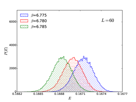
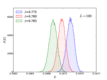
Figure 6: Histograms of the energy density, defined as $E=\langle H_{\rm RP}\rangle/L^{3}$, for three values of $\beta$ close to the critical point, for $L=60$ (top) and $L=100$ (bottom). To favor comparison, in both figures we use the same range of values of $E$, the same energy step, $\Delta E=10^{-5}$, and a similar number of energy measurements, of the order of $10^{5}$. There is no evidence of double peaks. Moreover, the width of the distributions decreases as $L$ increases, as expected at a continuous transition.

In order to estimate the exponent $\eta$, controlling the spatial decay of the two-point function $G(x)\sim|x|^{-1-\eta}$ at the critical point, we analyze the FSS behavior of the susceptibility, which is expected to be

$$\chi\approx L^{2-\eta}f_{\chi}(X).$$ (42)

A fit of the data using the estimates (41) gives $\eta=0.08(4)$, where the error takes also into account the uncertainty on $\beta_{c}$ and $\nu$. The corresponding scaling plot is reported in Fig. 5.

We also mention that analogous results are obtained by considering observables defined from the two-point function of the gauge invariant operators $P_{\bm{x}}^{ab}$, cf. Eq. (2), i.e. $G_{P}({\bm{x}}-{\bm{y}})=\langle{\rm Tr}\,P_{\bm{x}}^{\dagger}P_{\bm{y}}\rangle$. The staggered nature of the order parameter is taken into account be considering correlations only between even points, i.e., those such that $p_{\bm{x}}=(-1)^{\sum_{k}x_{k}}=1$.

This numerical study of the ARP³ lattice model provides a robust evidence that it undergoes a transition at a finite value of $\beta$.The obtained estimate of $\nu$ also allows us to exclude that the transition is of first order. Indeed, at a first-order transition FSS holds with $\nu=1/d=1/3$ NN-75 ; FB-82 ; PF-83 , while the estimate (41) of $\nu$ is definitely larger than $1/3$. To further confirm the continuous nature of the transition, we have also analyzed the distribution of the energy density, see Fig. 6. There is no evidence of two peaks and moreover, the width of the distributions decreases as $L$ increases, as expected at a continuous transition. Therefore, we conclude that the ARP³ lattice model undergoes a continuous transition, contradicting the predictions of the LGW theory.

It may be interesting to compare the estimate (41) of the correlation-length exponent $\nu$ with those of the 3D O($M$) vector models, which are $\nu=0.629971(4)$ for the Ising ($M=1$) universality class KPSV-16 ; Hasenbusch-10 ; CPRV-02 ; KP-17 ; GZ-98 , $\nu=0.6717(1)$ for the XY ($M=2$) universality class CHPV-06 ; KPSV-16 ; KP-17 ; GZ-98 , $\nu=0.7117(5)$ for the Heisenberg ($M=3$) universality class HV-11 ; CHPRV-02 ; GZ-98 , $\nu=0.749(2)$ for the O(4) universality class Hasenbusch-01 ; GZ-98 , $\nu=0.779(3)$ for the O(5) universality class HPV-05 ; FMSTV-05 , and $\nu\approx 1-c/M$ with $c=32/(3\pi^{2})$ for large $M$ ZJ-book . Our results are consistent with an Ising behavior. However, we do not have any theoretical argument for this identification, although we note that, at the transition, there is a breaking of the ${\mathbb{Z}}_{2}$ symmetry associated with the exchange of the even and odd sublattices.

V Conclusions

In this work we have studied the critical properties of the 3D antiferromagnetic RP^N-1 model, which is characterized by a global O($N$) symmetry and a discrete ${\mathbb{Z}}_{2}$ gauge symmetry. For this purpose we present field-theoretical perturbative calculations and extensive MC simulations.

In the LGW approach one first identifies the order parameter $\Phi$, then considers the most general $\Phi^{4}$ theory with the same symmetries as the original model, and finally determines the stable fixed points of the RG flow. If they correspond to a bare theory with the correct symmetry-breaking pattern, they characterize the possibly present continuous transitions. In the presence of gauge symmetries the method is usually applied by considering a gauge-invariant order parameter and a LGW field theory that is invariant under the global symmetries of the original model. In this LGW effective field theory the gauge degrees of freedom have been integrated out, implicitly assuming that they are not relevant for the dynamics of the critical modes. As already pointed out in Ref. PTV-17 , in some cases this assumption is not correct and the LGW approach may lead to erroneous conclusions on the nature of the critical behavior. For instance, this is the case of the 3D antiferromagnetic CP^N-1 model characterized by a U(1) gauge symmetry. In this paper we show that also in the case of ARP^N-1 models, which are invariant under a discrete gauge symmetry, the LGW approach based on a gauge invariant order parameter may give incorrect predictions on the critical behavior.

The LGW field theory of ARP^N-1 models is constructed using the staggered gauge-invariant composite operator, defined in Eq. (6). The LGW Hamiltonian does not present cubic terms due to the antiferromagnetic nearest-neighbor coupling which gives rise to an additional global ${\mathbb{Z}}_{2}$ symmetry. For $N=3$, the LGW approach nicely works: its nontrivial prediction of a symmetry enlargement of the leading critical behavior from O(3) to O(5) has been accurately verified numerically FMSTV-05 ; ACFJMRT-05 ; Carmona-etal-03 . However, for $N=4$, the LGW predictions disagree with the numerical results. The analyses of the RG flow using high-order perturbative series (five-loop series in the ${\overline{\rm MS}}$ renormalization scheme TV-72 and six-loop series in the massive zero-momentum scheme Parisi-80 ; ZJ-book ; PV-02 ) do not find any evidence of stable fixed points. This implies that any transition should be of first order. On the other hand, the numerical FSS analysis that we present for $N=4$ provides evidence of a continuous transition in the ARP³ model. This shows that LGW $\Phi^{4}$ theories constructed using a gauge-invariant order-parameter field do not generally capture the relevant features of the critical dynamics when the system has a discrete gauge symmetry.

These results are analogous to those reported in Ref. PTV-17 for systems with continuous gauge symmetries. In the presence of gauge symmetries, the main assumption of the LGW approach, i.e., that the transition is driven by gauge-invariant modes only, may be incorrect, so that the corresponding field theory may give erroneous predictions for the nature of the critical behavior. Therefore, critical gauge modes should be included to obtain an effective description of the critical behavior. For example, this happens in the large-$N$ limit of CP^N-1 lattice models PTV-17 , whose effective field-theoretical model is the abelian Higgs model for an $N$-component complex scalar field coupled to a dynamical U(1) gauge field MZ-03 . We believe that this point deserves further investigation.

The above considerations should be relevant for several interesting phase transitions in complex statistical systems. In particular we mention the finite-temperature transition of quantum chromodynamics (QCD). In the limit of $N_{f}$ massless quarks, the finite-temperature transition of QCD is related to the restoring of the chiral symmetry. The nature of the phase transition has been investigated within the LGW framework PW-84 ; Wilczek-92 ; RW-93 ; PV-13 ; BPV-03 , assuming that the relevant order-parameter field is a gauge-invariant quark operators, thus integrating out the gauge degrees of freedom. The present results show again that this assumption should not be taken for granted.

Appendix A High-order field-theoretical perturbative expansions

In this appendix we report the FT perturbative series of the $\beta$ functions used in our RG analysis of Sec. III. We only report results for $N=4$; the perturbative series for other values of $N$ are available on request.

The five-loop $\beta$ functions in the ${\overline{\rm MS}}$ scheme are

$$\beta_{u}(u,v) = -\epsilon u+\frac{17u^{2}}{6}+\frac{19uv}{12}+\frac{11v^{2}}{32}-\frac{41u^{3}}{12}-\frac{209u^{2}v}{72}-\frac{217uv^{2}}{192}-\frac{7v^{3}}{32}$$

$$+ \frac{67u^{4}\zeta(3)}{18}+\frac{13931u^{4}}{1728}+\frac{38}{9}u^{3}v\zeta(3)+\frac{38551u^{3}v}{3456}+\frac{39}{16}u^{2}v^{2}\zeta(3)+\frac{51059u^{2}v^{2}}{6912}+\frac{7}{8}uv^{3}\zeta(3)+\frac{44671uv^{3}}{18432}$$

$$+ \frac{145v^{4}\zeta(3)}{1152}+\frac{116401v^{4}}{442368}-\frac{1405u^{5}\zeta(5)}{54}-\frac{14311u^{5}\zeta(3)}{648}+\frac{1139\pi^{4}u^{5}}{19440}-\frac{1429027u^{5}}{62208}-\frac{4465}{108}u^{4}v\zeta(5)$$

$$- \frac{191273u^{4}v\zeta(3)}{5184}+\frac{6479\pi^{4}u^{4}v}{77760}-\frac{1261847u^{4}v}{31104}-\frac{42625u^{3}v^{2}\zeta(5)}{1296}-\frac{51007u^{3}v^{2}\zeta(3)}{1728}+\frac{7907\pi^{4}u^{3}v^{2}}{155520}$$

$$- \frac{17163385u^{3}v^{2}}{497664}-\frac{13555}{864}u^{2}v^{3}\zeta(5)-\frac{571493u^{2}v^{3}\zeta(3)}{41472}+\frac{775\pi^{4}u^{2}v^{3}}{41472}-\frac{16083989u^{2}v^{3}}{995328}-\frac{81835uv^{4}\zeta(5)}{20736}$$

$$- \frac{580207uv^{4}\zeta(3)}{165888}+\frac{2657\pi^{4}uv^{4}}{552960}-\frac{6769451uv^{4}}{1769472}-\frac{61675v^{5}\zeta(5)}{165888}-\frac{478109v^{5}\zeta(3)}{1327104}+\frac{12853\pi^{4}v^{5}}{19906560}-\frac{5857907v^{5}}{15925248}$$

$$+ \frac{164689u^{6}\zeta(7)}{864}+\frac{531683u^{6}\zeta(5)}{2592}-\frac{625u^{6}\zeta(3)^{2}}{864}+\frac{4204813u^{6}\zeta(3)}{41472}-\frac{23885\pi^{6}u^{6}}{326592}-\frac{88421\pi^{4}u^{6}}{207360}+\frac{49245733u^{6}}{663552}$$

$$+ \frac{218785}{576}u^{5}v\zeta(7)+\frac{553945u^{5}v\zeta(5)}{1296}-\frac{14041u^{5}v\zeta(3)^{2}}{5184}+\frac{53285101u^{5}v\zeta(3)}{248832}-\frac{276925\pi^{6}u^{5}v}{1959552}-\frac{801097\pi^{4}u^{5}v}{933120}$$

$$+ \frac{1971278291u^{5}v}{11943936}+\frac{194285}{512}u^{4}v^{2}\zeta(7)+\frac{17624591u^{4}v^{2}\zeta(5)}{41472}-\frac{103801u^{4}v^{2}\zeta(3)^{2}}{41472}+\frac{436868381u^{4}v^{2}\zeta(3)}{1990656}$$

$$- \frac{222605\pi^{6}u^{4}v^{2}}{1741824}-\frac{23850529\pi^{4}u^{4}v^{2}}{29859840}+\frac{17020433863u^{4}v^{2}}{95551488}+\frac{1078049u^{3}v^{3}\zeta(7)}{4608}+\frac{10457663u^{3}v^{3}\zeta(5)}{41472}$$

$$- \frac{120935u^{3}v^{3}\zeta(3)^{2}}{124416}+\frac{268220975u^{3}v^{3}\zeta(3)}{1990656}-\frac{3302315\pi^{6}u^{3}v^{3}}{47029248}-\frac{3326713\pi^{4}u^{3}v^{3}}{7464960}+\frac{3524497739u^{3}v^{3}}{31850496}$$

$$+ \frac{3219251u^{2}v^{4}\zeta(7)}{36864}+\frac{20008055u^{2}v^{4}\zeta(5)}{221184}-\frac{262619u^{2}v^{4}\zeta(3)^{2}}{995328}+\frac{1583254841u^{2}v^{4}\zeta(3)}{31850496}-\frac{9173555\pi^{6}u^{2}v^{4}}{376233984}$$

$$- \frac{25105729\pi^{4}u^{2}v^{4}}{159252480}+\frac{60138923803u^{2}v^{4}}{1528823808}+\frac{218981uv^{5}\zeta(7)}{12288}+\frac{3957851uv^{5}\zeta(5)}{221184}-\frac{58427uv^{5}\zeta(3)^{2}}{663552}$$

$$+ \frac{639020717uv^{5}\zeta(3)}{63700992}-\frac{1208975\pi^{6}uv^{5}}{250822656}-\frac{390793\pi^{4}uv^{5}}{11943936}+\frac{22934142763uv^{5}}{3057647616}+\frac{597163v^{6}\zeta(7)}{393216}$$

$$+ \frac{47034553v^{6}\zeta(5)}{31850496}-\frac{17285v^{6}\zeta(3)^{2}}{884736}+\frac{429887731v^{6}\zeta(3)}{509607936}-\frac{394585\pi^{6}v^{6}}{1003290624}-\frac{507587\pi^{4}v^{6}}{169869312}+\frac{4964312347v^{6}}{8153726976}\;,$$

$$\beta_{v}(u,v) = -\epsilon v+2uv+\frac{2v^{2}}{3}-\frac{127u^{2}v}{36}-\frac{191uv^{2}}{72}-\frac{89v^{3}}{192}$$

$$+ \frac{46}{9}u^{3}v\zeta(3)+\frac{5543u^{3}v}{864}+\frac{35}{6}u^{2}v^{2}\zeta(3)+\frac{24655u^{2}v^{2}}{3456}+\frac{53}{24}uv^{3}\zeta(3)+\frac{4705uv^{3}}{1536}+\frac{343v^{4}\zeta(3)}{1152}+\frac{29345v^{4}}{55296}$$

$$- \frac{1855}{54}u^{4}v\zeta(5)-\frac{1199}{48}u^{4}v\zeta(3)+\frac{1}{10}\pi^{4}u^{4}v-\frac{433597u^{4}v}{20736}-\frac{8525}{162}u^{3}v^{2}\zeta(5)-\frac{24923}{648}u^{3}v^{2}\zeta(3)+\frac{1543\pi^{4}u^{3}v^{2}}{9720}$$

$$- \frac{2047675u^{3}v^{2}}{62208}-\frac{41305u^{2}v^{3}\zeta(5)}{1296}-\frac{239593u^{2}v^{3}\zeta(3)}{10368}+\frac{163\pi^{4}u^{2}v^{3}}{1728}-\frac{10811653u^{2}v^{3}}{497664}-\frac{97445uv^{4}\zeta(5)}{10368}$$

$$- \frac{67753uv^{4}\zeta(3)}{10368}+\frac{577\pi^{4}uv^{4}}{23040}-\frac{2278937uv^{4}}{331776}-\frac{12335v^{5}\zeta(5)}{10368}-\frac{82787v^{5}\zeta(3)}{110592}+\frac{6251\pi^{4}v^{5}}{2488320}-\frac{12968855v^{5}}{15925248}$$

$$+ \frac{4753}{18}u^{5}v\zeta(7)+\frac{312229u^{5}v\zeta(5)}{1296}+\frac{313}{162}u^{5}v\zeta(3)^{2}+\frac{54641}{486}u^{5}v\zeta(3)-\frac{3415\pi^{6}u^{5}v}{30618}-\frac{106439\pi^{4}u^{5}v}{186624}$$

$$+ \frac{47092103u^{5}v}{746496}+\frac{36995}{72}u^{4}v^{2}\zeta(7)+\frac{90269}{192}u^{4}v^{2}\zeta(5)+\frac{8611u^{4}v^{2}\zeta(3)^{2}}{2592}+\frac{3045691u^{4}v^{2}\zeta(3)}{13824}-\frac{215305\pi^{6}u^{4}v^{2}}{979776}$$

$$- \frac{4203457\pi^{4}u^{4}v^{2}}{3732480}+\frac{748385887u^{4}v^{2}}{5971968}+\frac{81389}{192}u^{3}v^{3}\zeta(7)+\frac{1494113u^{3}v^{3}\zeta(5)}{3888}+\frac{47945u^{3}v^{3}\zeta(3)^{2}}{15552}$$

$$+ \frac{22766455u^{3}v^{3}\zeta(3)}{124416}-\frac{1048795\pi^{6}u^{3}v^{3}}{5878656}-\frac{6785357\pi^{4}u^{3}v^{3}}{7464960}+\frac{336567239u^{3}v^{3}}{2985984}+\frac{3438967u^{2}v^{4}\zeta(7)}{18432}$$

$$+ \frac{10313795u^{2}v^{4}\zeta(5)}{62208}+\frac{966247u^{2}v^{4}\zeta(3)^{2}}{497664}+\frac{39980171u^{2}v^{4}\zeta(3)}{497664}-\frac{2026955\pi^{6}u^{2}v^{4}}{26873856}-\frac{2808157\pi^{4}u^{2}v^{4}}{7464960}$$

$$+ \frac{2625960661u^{2}v^{4}}{47775744}+\frac{1612541uv^{5}\zeta(7)}{36864}+\frac{37924565uv^{5}\zeta(5)}{995328}+\frac{683903uv^{5}\zeta(3)^{2}}{995328}+\frac{9249647uv^{5}\zeta(3)}{497664}$$

$$- \frac{6338845\pi^{6}uv^{5}}{376233984}-\frac{19159367\pi^{4}uv^{5}}{238878720}+\frac{873191227uv^{5}}{63700992}+\frac{71197v^{6}\zeta(7)}{16384}+\frac{233623v^{6}\zeta(5)}{62208}+\frac{260705v^{6}\zeta(3)^{2}}{2654208}$$

$$+ \frac{57288493v^{6}\zeta(3)}{31850496}-\frac{1614635\pi^{6}v^{6}}{1003290624}-\frac{6779963\pi^{4}v^{6}}{955514880}+\frac{2063219231v^{6}}{1528823808}\;.$$

The six-loop $\beta$ functions in the MZM scheme are

$$\beta_{u}(u,v) = -u+{17\over 9}u^{2}+{19\over 18}uv+{11\over 48}v^{2}-1.02241u^{3}-0.86877u^{2}v-0.337791uv^{2}-0.0648148v^{3}\qquad$$

$$+ 1.10201u^{4}+1.46237u^{3}v+0.955215u^{2}v^{2}+0.324785uv^{3}+0.038265v^{4}-1.53069u^{5}-2.60142u^{4}v$$

$$- 2.1847u^{3}v^{2}-1.04534u^{2}v^{3}-0.254045uv^{4}-0.0237542v^{5}+2.50632u^{6}+5.35856u^{5}v+5.73074u^{4}v^{2}$$

$$+ 3.64914u^{3}v^{3}+1.35588u^{2}v^{4}+0.270658uv^{5}+0.0227444v^{6}-4.72398u^{7}-11.9943u^{6}v-15.2682u^{5}v^{2}$$

$$- 11.9206u^{4}v^{3}-5.84657u^{3}v^{4}-1.75721u^{2}v^{5}-0.297545uv^{6}-0.0218304v^{7}\;,$$

$$\beta_{v}(u,v) = -v+{4\over 3}uv+{4\over 9}v^{2}-1.05533u^{2}v-0.794696uv^{2}-0.140261v^{3}+1.02151u^{3}v$$

$$+ 1.14231u^{2}v^{2}+0.467669uv^{3}+0.0748728v^{4}-1.62911u^{4}v-2.52369u^{3}v^{2}-1.60381u^{2}v^{3}-0.497092uv^{4}$$

$$- 0.0617621v^{5}+2.62863u^{5}v+5.09733u^{4}v^{2}+4.34004u^{3}v^{3}+2.00838u^{2}v^{4}+0.491214uv^{5}+0.0495342v^{6}$$

$$- 5.29153u^{6}v-12.4905u^{5}v^{2}-13.3773u^{4}v^{3}-8.20642u^{3}v^{4}-2.97662u^{2}v^{5}-0.595112uv^{6}-0.0508251v^{7}\;.$$

Appendix B Summation of the pertubartive series

Since perturbative expansions are divergent, resummation methods must be used to obtain meaningful results. Given a generic quantity $S(u,v)$ with perturbative expansion $S(u,v)=\sum_{ij}c_{ij}u^{i}v^{j}$, we consider

$$S(xu,xv)=\sum_{k}s_{k}(u,v)x^{k},$$ (47)

which must be evaluated at $x=1$. The expansion (47) in powers of $x$ is resummed by using the conformal-mapping method ZJ-book that exploits the knowledge of the large-order behavior of the coefficients, generally given by

$$s_{k}(u,v)\sim k!\,[-A(u,v)]^{k}\,k^{b}\,\left[1+O(k^{-1})\right].$$ (48)

The quantity $A(u,v)$ is related to the singularity $t_{s}$ of the Borel transform $B(t)$ that is nearest to the origin: $t_{s}=-1/A(u,v)$. The series is Borel summable for $x>0$ if $B(t)$ does not have singularities on the positive real axis, and, in particular, if $A(u,v)>0$. The large-order behavior can be determined generalizing the discussion presented in Refs. LZ-77 ; ZJ-book . For even values of $N$, the expansion is Borel summable for

$$u+b_{N}v>0,\qquad u+\frac{1}{N}v>0,$$ (49)

where $b_{N}$ is given in Eq. (10). For odd $N$ we obtain analogously

$$u+b_{N}v>0,\qquad u+c_{N}v>0,$$ (50)

where $c_{N}$ is given in Eq. (12). Note that the conditions for Borel summability on the renormalized couplings correspond to the stability conditions (10) and (II) of the bare quartic couplings. In the Borel-summability region, for even values of $N$, the coefficient $A(u,v)$ is given by

$$A(u,v)=\frac{1}{2}\,{\rm Max}\left(u+b_{N}v,u+v/N\right).$$ (51)

For odd $N$, the same formula holds, replacing $u+v/N$ with $u+c_{N}v$. Under the additional assumption that the Borel-transform singularities lie only in the negative axis, the conformal-mapping method turns the original expansion into a convergent one in the region (49). Outside, the expansion is not Borel summable.

In the MZM scheme, the large-order behavior is still given by Eq. (48). For even $N$, we have

$$A(u,v)=a\;{\rm Max}\left(u+b_{N}v,u+v/N\right),$$ (52)

$$a=0.14777422...,$$

while, for odd values of $N$, $u+v/N$ should be replaced with $u+c_{N}v$.

Resummations are performed employing the conformal-mapping method, following closely Refs. ZJ-book ; CPV-00 . Resummations depend on two parameters ($\alpha$ and $b$ in the notations of Refs. ZJ-book ; CPV-00 ), which are optimized in the procedure.

References

• (1) L. D. Landau and E. M. Lifshitz, Statistical Physics. Part I, 3rd edition (Elsevier Butterworth-Heinemann, Oxford, 1980).
• (2) K. G. Wilson and J. Kogut, The renormalization group and the $\epsilon$ expansion, Phys. Rep. 12, 77 (1974).
• (3) M. E. Fisher, The renormalization group in the theory of critical behavior, Rev. Mod. Phys. 47, 543 (1975).
• (4) S.-k. Ma, Modern Theory of Critical Phenomena, (W.A. Benjamin, Reading, MA, 1976).
• (5) J. Zinn-Justin, Quantum Field Theory and Critical Phenomena, fourth edition (Clarendon Press, Oxford, 2002).
• (6) A. Pelissetto and E. Vicari, Critical Phenomena and Renormalization Group Theory, Phys. Rep. 368, 549 (2002).
• (7) A. Pelissetto, A. Tripodo, and E. Vicari, Landau-Ginzburg-Wilson approach to critical phenomena in the presence of gauge symmetries, Phys. Rev. D 96, 034505 (2017).
• (8) F. Delfino, A. Pelissetto, and E. Vicari, Three-dimensional antiferromagnetic CPN-1 models, Phys. Rev. E 91, 052109 (2015).
• (9) A. Nahum, J. T. Chalker, P. Serna, M. Ortuno, and A. M. Somoza, 3D Loop Models and the CPN-1 Sigma Model, Phys. Rev. Lett. 107, 110601 (2011); Phase transitions in three-dimensional loop models and the CPN-1 sigma model, Phys. Rev. B 88, 134411 (2013).
• (10) J. L. Alonso, A. Cruz, L. A. Fernandez, S. Jimenez, V. MartΓ­n-Mayor, J.J. Ruiz-Lorenzo, and A. TarancΓ³n, Phase diagram of the bosonic double-exchange model, Phys. Rev. B 71, 014420 (2005).
• (11) L. A. Fernandez, V. MartΓ­n-Mayor, D. Sciretti, A. TarancΓ³n, and J. L. Velasco, Numerical study of the enlarged O(5) symmetry of the 3D antiferromagnetic RP2 spin model, Phys. Lett. B 628, 281 (2005).
• (12) J. M. Carmona, A. Cruz, L. A. Fernandez, S. Jimenez, V. MartΓ­n-Mayor, A. MuΓ±oz-Sudupe, J. Pech, J. J. Ruiz-Lorenzo, A. TarancΓ³n, and P. Tellez, Dynamical generation of a gauge symmetry in the Double-Exchange model, Phys. Lett. B 560, 140 (2003).
• (13) G. ’t Hooft and M. J. G. Veltman, Regularization and renormalization of gauge fields, Nucl. Phys. B 44, 189 (1972).
• (14) K. G.Β Wilson and M. E.Β Fisher, Critical exponents in 3.99 dimensions, Phys. Rev. Lett. 28, 240 (1972).
• (15) P. Calabrese, A. Pelissetto, and E. Vicari, Multicritical behavior of O$(n_{1})$ $\oplus$O$(n_{2})$-symmetric systems, Phys. Rev. B 67, 054505 (2003).
• (16) J. Carmona, A. Pelissetto, and E. Vicari, The $N$-component Ginzburg-Landau Hamiltonian with cubic symmetry: a six-loop study, Phys. Rev. B 61, 15136 (2000).
• (17) M. Hasenbusch and E. Vicari, Anisotropic perturbations in 3D O(N) vector models, Phys. Rev. B 84, 125136 (2011).
• (18) S. Mo, J. Hove, and A. SudbΓΈ, Order of the metal-to-superconductor transition, Phys. Rev. B 65, 104501 (2002).
• (19) F. S. Nogueira and H. Kleinert, in Order, Disorder, and Criticality, edited by Y. Holovatch (World Scientific, Singapore, 2007); arXiv:cond-mat/0303485.
• (20) C. W. Garland and G. Nounesis, Critical behavior at nematic-smectic-A phase transitions, Phys. Rev. E 49, 2964 (1994).
• (21) B.I. Halperin, T.C. Lubensky, and S.K. Ma, First-order phase transitions in superconductors and smectic-A liquid crystals, Phys. Rev. Lett. 32, 292 (1974).
• (22) P. Calabrese, P. Parruccini, A. Pelissetto, and E. Vicari, Critical behavior of O(2)$\otimes$O($N$)-symmetric models, Phys. Rev. B 70, 174439 (2004).
• (23) Y. Nakayama and T. Ohtsuki, Bootstrapping phase transitions in QCD and frustrated spin systems, Phys. Rev. D 91, 021901(R) (2015).
• (24) M. De Prato, A. Pelissetto, and E. Vicari, The normal-to-planar superfluid transition in 3He, Phys. Rev. B 70, 214519 (2004).
• (25) R. D. Pisarski and F. Wilczek, Remarks on the chiral phase transition in chromodynamics, Phys. Rev. D 29, 338 (1984).
• (26) A. Pelissetto and E. Vicari, Relevance of the axial anomaly at the finite-temperature chiral transition in QCD, Phys. Rev. D 88, 105018 (2013).
• (27) V.Β Dohm, Nonuniversal Critical Phenomena along the Lambda Line of 4He: I. Specific Heat in Three Dimensions, Z. Phys. B 60, 61 (1985); Nonuniversal Critical Phenomena along the Lambda Line of 4He: II. Thermal Conductivity in Three Dimensions, Z. Phys. B 61, 193 (1985).
• (28) R.Β Schloms and V.Β Dohm, Minimal renormalization without $\epsilon$-expansion: Critical behavior in three dimensions, Nucl. Phys. B 328, 639 (1989).
• (29) J. C. Le Guillou and J. Zinn-Justin, Critical exponents for thr $n$-vector model in three dimensions from field theory, Phys.Β Rev.Β Lett. 39, 95 (1977); Critical exponents from field theory, Phys.Β Rev. B 21, 3976 (1980).
• (30) G.Β Parisi, Field-theoretic approach to second-order phase transitions in two- and three-dimensional systems, CargΓ¨se Lectures (1973); J. Stat. Phys. 23, 49 (1980).
• (31) A. Pelissetto and E. Vicari, Four-point renormalized coupling constant and Callan-Symanzik $\beta$-function in O(N) models, Nucl. Phys. B 519, 626 (1998); P. Calabrese, M. Caselle, A. Celi, A. Pelissetto, and E. Vicari, Nonanalyticity of the Callan-Symanzik $\beta$-function of two-dimensional O($N$) models, J. Phys. A 33, 8155 (2000).
• (32) The update of the spin $s_{\bf x}$ consists in proposing the new vector $R\,s_{\bf x}$, where $R$ is a random O(2) matrix acting on two randomly chosen components of $s_{\bf x}$. Then we perform the standard Metropolis acceptance check, tuning the parameters to have an acceptance probability of about 30%.
• (33) B. Nienhuis and M. Nauenberg, First-order phase transitions in renormalization-group theory, Phys. Rev. Lett. 35, 477 (1975).
• (34) M. E. Fisher and A. N. Berker, Scaling for first-order phase transitions in thermodynamic and finite systems, Phys. Rev. B 26, 2507 (1982).
• (35) V. Privman and M. E. Fisher, Finite-size effects at first-order transitions, J. Stat. Phys. 33, 385 (1983).
• (36) F. Kos, D. Poland, D. Simmons-Duffin, and A. Vichi, Precision islands in the Ising and O($N$) models, J. High Energy Phys. 08, 036 (2016).
• (37) M. Hasenbusch, A finite size scaling study of lattice models in the three-dimensional Ising universality class, Phys. Rev. B 82, 174433 (2010).
• (38) M. Campostrini, A. Pelissetto, P. Rossi, and E. Vicari, 25th-order high-temperature expansion results for three-dimensional Ising-like systems on the simple-cubic lattice Phys. Rev. E 65, 066127 (2002).
• (39) M. V. Kompaniets and E. Panzer, Minimally subtracted six-loop renormalization of O($n$)-symmetric $\varphi^{4}$ theory and critical exponents, Phys. Rev. D 96, 036016 (2017).
• (40) R. Guida and J. Zinn-Justin, Critical exponents of the N-vector model, J. Phys. A 31, 8103 (1998).
• (41) M. Campostrini, M. Hasenbusch, A. Pelissetto, and E. Vicari, Theoretical estimates of the critical exponents of the superfluid transition in 4He by lattice methods, Phys. Rev. B 74, 144506 (2006).
• (42) M. Campostrini, M. Hasenbusch, A. Pelissetto, P. Rossi, and E. Vicari, Critical exponents and equation of state of the three-dimensional Heisenberg universality class, Phys. Rev. B 65, 144520 (2002).
• (43) M.Β Hasenbusch, Eliminating leading corrections to scaling in the three-dimensional O($N$)-symmetric $\Phi^{4}$ model: $N$ = 3 and 4, J. Phys. A 34, 8221 (2001).
• (44) M. Hasenbusch, A. Pelissetto, and E. Vicari, Instability of O(5) multicritical behavior in SO(5) theory of high- $T_{c}$ superconductors, Phys. Rev. B 72, 014532 (2005).
• (45) M. Moshe and J. Zinn-Justin, Quantum field theory in the large $N$ limit: A review, Phys. Rep. 385, 69 (2003).
• (46) F. Wilczek, Application of the renormalization group to a second-order QCD phase transition, Int. J. Mod. Phys. A 7, 3911 (1992).
• (47) K. Rajagopal and F. Wilczek, Static and dynamic critical phenomena at a second order QCD phase transition, Nucl. Phys. B 399, 395 (1993).
• (48) A. Butti, A. Pelissetto, and E. Vicari, On the nature of the finite-temperature chiral transition in QCD, J. High Energy Phys. 08, 029 (2003); F. Basile, A. Pelissetto, and E. Vicari, The finite-temperature chiral transition in QCD with adjoint fermions, J. High Energy Phys. 02, 044 (2005).