Multidimensional entropic uncertainty relation based on a commutator matrix
in position and momentum spaces

Abstract

The uncertainty relation for continuous variables due to Byalinicki-Birula and Mycielski expresses the complementarity between two $n$-tuples of canonically conjugate variables $(x_{1},x_{2},\cdots x_{n})$ and $(p_{1},p_{2},\cdots p_{n})$ in terms of Shannon differential entropy. Here, we consider the generalization to variables that are not canonically conjugate and derive an entropic uncertainty relation expressing the balance between any two $n$-variable Gaussian projective measurements. The bound on entropies is expressed in terms of the determinant of a matrix of commutators between the measured variables. This uncertainty relation also captures the complementarity between any two incompatible linear canonical transforms, the bound being written in terms of the corresponding symplectic matrices in phase space. Finally, we extend this uncertainty relation to Rényi entropies and also prove a covariance-based uncertainty relation which generalizes Robertson relation.

I Introduction

At the heart of quantum mechanics, uncertainty relations reflect the impossibility to define – exactly and simultaneously – the value of two observables that do not commute, such as the position $\hat{x}$ and momentum $\hat{p}$ of a particle. Uncertainty relations, expressed in terms of variances of observables, were first introduced by Heisenberg Heisenberg and Kennard Kennard , and then generalized by Schrödinger Schrodinger and Robertson Robertson . Later on, it was shown by Hirschman Hirschman that uncertainty relations may also be formulated in terms of Shannon entropies instead of variances, leading to the first entropic uncertainty relation for canonically conjugate variables $\hat{x}$ and $\hat{p}$ proven by Bialynicki-Birula and Mycielski Birula and Beckner Beckner . Entropic uncertainty relations have also been developed for discrete observables in finite-dimensional spaces, see Coles for a review, but here we focus on continuous-spectrum observables in an infinite-dimensional space. Specifically, we use the notations of quantum optics and view variables $\hat{x}$ and $\hat{p}$ as canonically conjugate quadrature components of a bosonic mode. Then, the $n$-modal version of the entropic uncertainty relation for the $n$-tuples $\vec{x}=(x_{1},x_{2},\cdots x_{n})$ and $\vec{p}=(p_{1},p_{2},\cdots p_{n})$ is expressed asBirula

$$h(\vec{x})+h(\vec{p})\geq n\ln(\pi e)$$ (1)

where $h(\vec{x})$ and $h(\vec{p})$ are the Shannon differential entropies of $\vec{x}$ and $\vec{p}$, namely

$$h(\vec{x})\equiv h(|\psi(\vec{x})|^{2}) = -\int d\vec{x}\;|\psi(\vec{x})|^{2}\ln|\psi(\vec{x})|^{2},$$

$$h(\vec{p})\equiv h(|\phi(\vec{p})|^{2}) = -\int d\vec{p}\;|\phi(\vec{p})|^{2}\ln|\phi(\vec{p})|^{2},$$ (2)

with $|\psi(\vec{x})|^{2}=|\langle x_{1},x_{2},\cdots x_{n}|\psi\rangle|^{2}$ and $|\phi(\vec{p})|^{2}=|\langle p_{1},p_{2},\cdots p_{n}|\psi\rangle|^{2}$ being the probability distributions of $\vec{x}$ and $\vec{p}$ in the pure state $|\psi\rangle$. Of course, $\phi(\vec{p})$ is the Fourier transform of $\psi(\vec{x})$, which is at the origin of the complementarity between $\vec{x}$ and $\vec{p}$ expressed by Eq. (1). Lately, this entropic uncertainty relation has been extended by taking $x$-$p$ correlations into account hertz , the significant advantage being that the resulting uncertainty relation is saturated by any pure $n$-modal Gaussian state.

In 2011, Huang huang generalized the entropic uncertainty relation to a pair of observables that are not canonically conjugate. More precisely, defining the observables

$$\hat{A}=\sum_{i=1}^{n}(a_{i}\,\hat{x}_{i}+a_{i}^{\prime}\,\hat{p}_{i}),\quad\hat{B}=\sum_{i=1}^{n}(b_{i}\,\hat{x}_{i}+b_{i}^{\prime}\,\hat{p}_{i}),$$ (3)

he showed that

$$h(\hat{A})+h(\hat{B})\geq\ln(\pi e|[\hat{A},\hat{B}]|)$$ (4)

where $[\hat{A},\hat{B}]$ (which is a scalar) is the commutator between both observables. Obviously, if $\hat{A}=\hat{x}$ and $\hat{B}=\hat{p}$, this inequality reduces to Eq. (1). In addition, a similar result had earlier been obtained by Guanlei et al. Guanlei in the special case where $n=1$, namely

$$h(\hat{x}_{\theta})+h(\hat{x}_{\phi})\geq\ln(\pi e|\sin(\theta-\phi)|)$$ (5)

where $\hat{x}_{\theta}=\hat{x}\cos\theta+\hat{p}\sin\theta$ and $\hat{x}_{\phi}=\hat{x}\cos\phi+\hat{p}\sin\phi$ are two rotated quadratures.

In this paper, we introduce a generalization of the uncertainty relation of Byalinicki-Birula and Mycielski, which is stated in the form of our Theorem 1. It addresses the situation where $n$ arbitrary quadratures are jointly measured on $n$ modes, expressing the balance between two such joint measurements (see Fig. 1). In other words, we state an entropic uncertainty relation between two arbitrary $n$-modal Gaussian projective measurements (or, equivalently, two $n$-mode Gaussian unitaries $U_{A}$ and $U_{B}$). The lower bound of our uncertainty relation, Eq. (32), depends on the determinant of a $n\times n$ matrix formed with the commutators between the $n$ measured quadratures in both cases. In contrast, Eq. (1) is restricted to the case of measuring either all $x$ quadratures or all $p$ quadratures on $n$ modes, while Refs. huang ; Guanlei treat the balance between two single-mode measurements only.

Interestingly, the probability distribution of the measured quadratures is given by the squared modulus of the linear canonical transform (LCT) associated with $U_{A}$ or $U_{B}$, so that our entropic uncertainty relation also captures the complementarity between two incompatible $n$-dimensional LCTs as expressed by our Lemma 1. It simply reduces to Eq. (1) when the two LCTs are connected by a $n$-dimensional Fourier transform, mapping $\vec{x}=(x_{1},x_{2},\cdots x_{n})^{T}$ onto $\vec{p}=(p_{1},p_{2},\cdots p_{n})^{T}$.

In Section II, we define general $n$-dimensional LCT’s and give some useful properties. Section III presents our results on uncertainty relations for $n$ modes. First, we derive a generalized entropic uncertainty relation based on differential Shannon entropies (our Theorem 1, with its extension to a larger-dimensional space), then we extend it to Rényi entropies (our Theorem 2), and finally we exhibit a covariance-based uncertainty relation (our Theorem 3). In Section IV, we conclude and suggest a conjecture for a generalized entropic uncertainty relation in the case where the commutators differ from scalars.

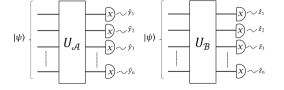
Figure 1: Schematic of two $n$-modal Gaussian projective measurements applied onto state $|\psi\rangle$, resulting in the $n$ quadratures $\hat{y}_{i}$’s or $\hat{z}_{i}$’s. These measurements can be implemented by applying a Gaussian unitary ($U_{A}$ or $U_{B}$) onto $|\psi\rangle$ and measuring the $\hat{x}$-quadratures of the $n$ modes. Our uncertainty relation, Eq. (32), expresses the complementarity between the $\hat{y}_{i}$’s and $\hat{z}_{i}$’s, or equivalently between the linear canonical transforms associated with $U_{A}$ and $U_{B}$.

II Linear canonical transforms

Before deriving our uncertainty relations, we need to properly define fractional Fourier transforms (FRFTs) along with their generalization to LCTs. Some early papers on FRFTs appeared in the 1920’s, but this topic became investigated in depth only more recently in the fields of signal processing and quantum optics (see, e.g., Pei ; Bultheel ; Morsche ; Ozaktasbook ; Ozaktas for more details). In one dimension, the FRFT of a wave function $f(x)$ can be understood as the new wave function obtained when the Wigner function corresponding to $f(x)$ undergoes a rotation of angle $\alpha$ in phase space. If $\alpha=\pi/2$, then the FRFT simply coincides with the usual Fourier transform, connecting the time and frequency domains in the field of signal processing or the canonically conjugate $x$- and $p$-quadratures in quantum optics. Mathematically, the one-dimensional FRFT of function $f(x)$ is defined as

$$\mathcal{F}_{\alpha}(y)=\sqrt{\frac{1-i\cot\alpha}{2\pi}}\;e^{\frac{i}{2}y^{2}\cot\alpha}\int e^{\frac{-iyx}{\sin\alpha}}e^{\frac{i}{2}x^{2}\cot\alpha}f(x)\,dx$$ (6)

The one-dimensional FRFT can be generalized to one-dimensional LCTs by including all affine linear transformations in phase space $(x,p)$, going beyond rotations. Accordingly, the LCT of wave function $f(x)$ is the new wave function obtained when the corresponding Wigner function undergoes a symplectic transformation $\mathcal{S}$. The one-dimensional LCT of $f(x)$ is defined as

$$\mathcal{F}_{\mathcal{S}}(y)=\sqrt{\frac{1}{2\pi ib}}\;e^{\frac{id}{2b}y^{2}}\int e^{\frac{-iyx}{b}}e^{\frac{ia}{2b}x^{2}}f(x)\,dx$$ (7)

where $\mathcal{S}=\begin{pmatrix}a&b\\ c&d\end{pmatrix}$ is a symplectic matrix with $a$, $b$, $c$, and $d$ being real parameters, and $b\neq 0$.

The notion of LCT can readily be extended to $n$ dimensions, the resulting transformation being also sometimes called $n$-dimensional FRFT. The physical interpretation is straightforward, namely a LCT is the transformation of a $n$-dimensional wave function $f(\vec{x})$ that is effected by any symplectic transformation in the $2n$-dimensional phase space of variables $(x_{1},x_{2},\cdots x_{n})$ and $(p_{1},p_{2},\cdots p_{n})$. We write the symplectic matrix $\mathcal{S}$ as

$$\mathcal{S} = \begin{pmatrix}a&b\\ c&d\end{pmatrix}$$ (8)

$$= \begin{pmatrix}\mathds{1}&0\\ db^{-1}&\mathds{1}\end{pmatrix}\begin{pmatrix}b&0\\ 0&b^{-1}\end{pmatrix}\begin{pmatrix}0&\mathds{1}\\ -\mathds{1}&0\end{pmatrix}\begin{pmatrix}\mathds{1}&0\\ b^{-1}a&\mathds{1}\end{pmatrix}$$

where $a$, $b$, $c$, and $d$ are $n\times n$ real matrices, $\openone$ is the $n\times n$ identity matrix, and $\det(b)\neq 0$. Since $\mathcal{S}$ is symplectic, it obeys the constraint

$$\mathcal{S}J\mathcal{S}^{T}=J\mathrm{\leavevmode\nobreak\ \leavevmode\nobreak\ \leavevmode\nobreak\ \leavevmode\nobreak\ \leavevmode\nobreak\ with\leavevmode\nobreak\ }J=\begin{pmatrix}0&\mathds{1}\\ -\mathds{1}&0\end{pmatrix}$$ (9)

being the symplectic form, so that $\det(S)=1$. This also implies that $ab^{T}$ and $cd^{T}$ are symmetric matrices, and $ad^{T}-bc^{T}=\mathds{1}$. The corresponding symplectic transformation in phase space is

$$\begin{pmatrix}\vec{y}\\ \vec{q}\end{pmatrix}=\mathcal{S}\begin{pmatrix}\vec{x}\\ \vec{p}\end{pmatrix},$$ (10)

where $\vec{y}=(y_{1},y_{2},\cdots y_{n})^{T}$ and $\vec{q}=(q_{1},q_{2},\cdots q_{n})^{T}$ form a new pair of canonically conjugate $n$-tuples. In state space, the LCT of $f(\vec{x})$ can be written as

$$\mathcal{F}_{\mathcal{S}}[f(\vec{x})](\vec{y}) = \frac{1}{\sqrt{(2\pi)^{n}|\det(b)|}}\int d\vec{x}f(\vec{x})\,e^{-i\,b^{-1}\vec{y}\cdot\vec{x}}$$ (11)

$$\leavevmode\nobreak\ \leavevmode\nobreak\ \leavevmode\nobreak\ \leavevmode\nobreak\ \leavevmode\nobreak\ \leavevmode\nobreak\ \times\;e^{\frac{i}{2}\left[\vec{x}^{T}(b^{-1}a)\vec{x}+\vec{y}^{T}(db^{-1})\vec{y}\right]}$$

$$= C_{db^{-1}}D_{b^{-1}}\mathcal{F}C_{b^{-1}a}[f(\vec{x})](\vec{y})$$

with

$$C_{r}[f](\vec{x}) = e^{\frac{i}{2}\vec{x}^{T}r\vec{x}}f(\vec{x})$$

$$D_{b}[f](\vec{x}) = \sqrt{|\det(b)|}f(b\,\vec{x})$$

$$\mathcal{F}[f](\vec{x}) = \frac{1}{(2\pi)^{n/2}}\int d\vec{y}f(\vec{y})e^{-i\,\vec{x}\cdot\vec{y}}$$ (12)

where $C_{r}$ represents the chirp multiplication, $D_{b}$ the squeezing (or dilation) operator, and $\mathcal{F}$ the usual Fourier transform. These operators are directly related to the decomposition of $\mathcal{S}$ in Eq. (8). Note also that the chirp multiplication (in one dimension) can be expressed as a product of the other two operators, namely $C_{r}=R_{\theta-\pi/2}\cdot D_{\tan\theta}\cdot R_{\theta}$ where $R_{\theta}$ represent the rotation and $r=\tan\theta-\cot\theta$. Finally, note that the set of LCTs in phase space is in one-to-one correspondence with the set of Gaussian unitaries in state space weedbrook , which can indeed be decomposed into passive linear-optics operations (phase shifters and beam splitters, i.e., rotations in phase space) and active squeezing operations (i.e., area-preserving dilations in phase space).

Here are some properties of LCTs that will be useful to prove our results in Section III.

Properties.

1. $\mathcal{F}_{\mathcal{A}}\mathcal{F}_{\mathcal{B}}=\mathcal{F}_{\mathcal{AB}}$

2. $D_{b_{1}}D_{b_{2}}=D_{b_{1}b_{2}}$

3. $\mathcal{F}^{-1}=D_{-1}\mathcal{F}$ where $\mathcal{F}^{-1}$ is the inverse Fourier transform.

4. $\left|C_{r}\,f\right|=\left|f\right|$

Proof.

1. Using Eq. (11) and the corresponding representation in phase space, Eq. (8), we see that $\mathcal{F}_{\mathcal{A}}\mathcal{F}_{\mathcal{B}}$ is represented by the matrix $\mathcal{AB}$. Since the symplectic matrices form a group, the product of two symplectic matrices is a symplectic matrix, which also admits decomposition (8) and thus represents the linear canonical transform $\mathcal{F_{AB}}$.

Proofs of 2, 3 and 4 are straightforward. ∎

III Multidimensional uncertainty relations

III.1 Entropic uncertainty relation between two linear canonical transforms

Let $|\psi\rangle$ be an arbitrary $n$-mode state. We wish to express the complementarity between two incompatible LCTs corresponding to two Gaussian unitaries ($U_{A}$ or $U_{B}$) applied onto $|\psi\rangle$. As shown in Fig. 1, we measure in both cases the $n$-tuple of output $x$-quadratures, which corresponds to applying two possible $n$-modal Gaussian projective measurements on $|\psi\rangle$. The vectors of measurement outcomes are noted, respectively, $\vec{y}=(y_{1},\cdots,y_{n})^{T}$ or $\vec{z}=(z_{1},\cdots,z_{n})^{T}$. Denoting as $\mathcal{A}$ and $\mathcal{B}$ the symplectic transformations associated with $U_{A}$ and $U_{B}$, and writing as $\hat{r}=(\hat{x}_{1},\cdots,\hat{x}_{n},\hat{p}_{1},\cdots,\hat{p}_{n})^{T}$ the $2n$-dimensional vector of input quadratures, we may express the corresponding vectors of output quadratures as

$$\hat{r}_{A}=\mathcal{A}\;\hat{r}\equiv\begin{pmatrix}\vec{y}\\ \vec{q}\end{pmatrix},\quad\hat{r}_{B}=\mathcal{B}\;\hat{r}\equiv\begin{pmatrix}\vec{z}\\ \vec{o}\end{pmatrix}.$$ (13)

where $\vec{q}$ (resp. $\vec{o}$) is the vector of quadratures that are canonically conjugate with $\vec{y}$ (resp. $\vec{z}$). The probability distributions for $\vec{y}$ and $\vec{z}$ are thus given by the squared modulus of the LCTs associated with $U_{A}$ and $U_{B}$, namely $\left|\mathcal{F}_{\mathcal{A}}[\psi(\vec{x})](\vec{y})\right|^{2}$ and $\left|\mathcal{F}_{\mathcal{B}}[\psi(\vec{x})](\vec{z})\right|^{2}$. In order to find an entropic uncertainty relation for $\vec{y}$ and $\vec{z}$, we first express the complementarity between $\mathcal{F}_{\mathcal{A}}$ and $\mathcal{F}_{\mathcal{B}}$ in the following Lemma.

Lemma 1.

Let $\mathcal{F}_{\mathcal{A}}$ and $\mathcal{F}_{\mathcal{B}}$ be two LCTs of a function $f(\vec{x})$ with $\vec{x}=(x_{1},\cdots x_{n})$. Then, their squared moduli satisfy the entropic uncertainty relation

$$h(|\mathcal{F}_{\mathcal{A}}|^{2})+h(|\mathcal{F}_{\mathcal{B}}|^{2})\geq\ln\left((\pi e)^{n}|\det(\mathcal{B}_{b}\mathcal{A}_{a}^{T}-\mathcal{B}_{a}\mathcal{A}_{b}^{T})|\right)$$ (14)

where

$$\mathcal{A}=\begin{pmatrix}\mathcal{A}_{a}&\mathcal{A}_{b}\\ \mathcal{A}_{c}&\mathcal{A}_{d}\end{pmatrix}\quad\text{and}\quad\mathcal{B}=\begin{pmatrix}\mathcal{B}_{a}&\mathcal{B}_{b}\\ \mathcal{B}_{c}&\mathcal{B}_{d}\end{pmatrix}$$ (15)

are the symplectic matrices associated with $\mathcal{F}_{\mathcal{A}}$ and $\mathcal{F}_{\mathcal{B}}$ [acting on the quadrature operators as in Eq. (13)] and $h(\cdot)$ denotes Shannon differential entropy.

Proof.

Let us define the function

$$G\left(\vec{x}\right)=C_{-b^{-1}a}\,\mathcal{F}_{\mathcal{A}}(\vec{x})=e^{-\frac{i}{2}\vec{x}^{T}(b^{-1}a)\vec{x}}\,\mathcal{F}_{\mathcal{A}}\left(\vec{x}\right).$$ (16)

The inverse Fourier transform of $G(\vec{x})$ is

$$g\left(\vec{p}\right)=\mathcal{F}^{-1}[G\left(\vec{x}\right)](\vec{p})=\left[D_{-1}\mathcal{F}\,G\right]\left(\vec{p}\right),$$ (17)

where the second equality results from property 3. Since $\left|G\left(\vec{x}\right)\right|^{2}=\left|\mathcal{F}_{\mathcal{A}}\left(\vec{x}\right)\right|^{2}$, the probability distributions are equal, so that $h\left(\left|G\left(\vec{x}\right)\right|^{2}\right)=h\left(\left|\mathcal{F}_{\mathcal{A}}\left(\vec{x}\right)\right|^{2}\right)$. Then, we may apply Eq. (1) to $G$ and $g$, which gives

$$h\left(\left|\mathcal{F}_{\mathcal{A}}\left(\vec{x}\right)\right|^{2}\right)+h\left(\left|g\left(\vec{p}\right)\right|^{2}\right)\geq n\ln(\pi e).$$ (18)

With the change of variables $\vec{p}\rightarrow b^{-1}\vec{p}$, we have

$$h\left(\left|g\left(\vec{p}\right)\right|^{2}\right) = -\int\left|g\left(\vec{p}\right)\right|^{2}\ln\left|g\left(\vec{p}\right)\right|^{2}d\vec{p}$$ (19)

$$= -\int\left|g\left(b^{-1}\vec{p}\right)\right|^{2}\ln\left|g\left(b^{-1}\vec{p}\right)\right|^{2}\frac{d\vec{p}}{|\det(b)|}.\qquad$$

By using the above properties of LCTs, we have

$$\left|g\left(b^{-1}\vec{p}\right)\right|^{2} = \left|\sqrt{\det(b)}\;D_{b^{-1}}\left[g\right]\left(\vec{p}\right)\right|^{2}$$ (20)

$$= |\det(b)|\;\big{|}\left[D_{b^{-1}}D_{-1}\mathcal{F}\,G\right]\left(\vec{p}\right)\big{|}^{2}$$

$$= |\det(b)|\;\big{|}\left[D_{b^{-1}}D_{-1}\mathcal{F}\,C_{-b^{-1}a}\mathcal{F}_{\mathcal{A}}\right]\left(\vec{p}\right)\big{|}^{2}$$

$$= |\det(b)|\;\big{|}\left[C_{-db^{-1}}D_{{-b^{-1}}}\mathcal{F}\,C_{-b^{-1}a}\mathcal{F}_{\mathcal{A}}\right]\left(\vec{p}\right)\big{|}^{2}$$

$$= |\det(b)|\;\left|\left[\mathcal{F}_{\mathcal{S}_{\ominus}}\mathcal{F}_{\mathcal{A}}\right]\left(\vec{p}\right)\right|^{2}$$

$$= |\det(b)|\left|\left[\mathcal{F}_{\mathcal{S}_{\ominus}\mathcal{A}}\right]\left(\vec{p}\right)\right|^{2},$$

where we have defined $\mathcal{S}_{\ominus}=\left(\begin{array}[]{cc}a&-b\\ -c&d\end{array}\right)$, so by plugging it into Eq. (19), we get

$$h\left(|g\left(\vec{p}\right)|^{2}\right) = h\left(|\mathcal{F}_{\mathcal{S}_{\ominus}\mathcal{A}}\left(\vec{p}\right)|^{2}\right)-\ln|\det(b)|$$ (21)

since $|\mathcal{F}_{\mathcal{S}_{\ominus}\mathcal{A}}|^{2}$ is a normalized function. Now, replacing $h\left(|g\left(\vec{p}\right)|^{2}\right)$ in Eq. (18), we obtain

$$h\left(\left|\mathcal{F}_{\mathcal{A}}\left(\vec{x}\right)\right|^{2}\right)+h\left(|\mathcal{F}_{\mathcal{S}_{\ominus}\mathcal{A}}\left(\vec{p}\right)|^{2}\right)\geq\ln((\pi e)^{n}|\det(b)|).$$ (22)

The last step is simply to define $\mathcal{B}=\mathcal{S}_{\ominus}\mathcal{A}$ or equivalently $\mathcal{S}_{\ominus}=\mathcal{B}\mathcal{A}^{-1}$. Since symplectic matrices form a group and $\mathcal{A}$ and $\mathcal{B}$ are symplectic, $\mathcal{S}_{\ominus}$ is necessarily symplectic too. The property that $\mathcal{A}$ is symplectic translates into

$$\mathcal{A}^{-1}=J\mathcal{A}^{T}J^{T}=\begin{pmatrix}\mathcal{A}_{d}^{T}&-\mathcal{A}_{b}^{T}\\ -\mathcal{A}_{c}^{T}&\mathcal{A}_{a}^{T}\end{pmatrix},$$ (23)

hence $b=\mathcal{B}_{a}\mathcal{A}_{b}^{T}-\mathcal{B}_{b}\mathcal{A}_{a}^{T}$. Replacing $b$ into Eq. (22) completes the proof of Eq. (14), which thus provides a $n$-dimensional entropic uncertainty relation for any two incompatible LCTs. ∎

Note that in the special case of one mode ($n=1$), we recover the result obtained by Guanlei et al. Guanlei2 for one-dimensional LCTs, namely

$$h(|\mathcal{F}_{\mathcal{A}}|^{2})+h(|\mathcal{F}_{\mathcal{B}}|^{2})\geq\ln\left(\pi e|ab^{\prime}-a^{\prime}b|\right)$$ (24)

for two $2\times 2$ matrices $\mathcal{A}=\begin{pmatrix}a&b\\ c&d\end{pmatrix}$ and $\mathcal{B}=\begin{pmatrix}a^{\prime}&b^{\prime}\\ c^{\prime}&d^{\prime}\end{pmatrix}$ (see Eq. (20) in Ref. Guanlei2 ). Furthermore, for one-dimensional FRFTs (when $\mathcal{A}$ and $\mathcal{B}$ are simply rotations), we recover Eq. (5) (see Eq. (15) in Ref. Guanlei ). Now, back to the $n$-mode case, if we choose $\mathcal{A}=\mathds{1}$ and $\mathcal{B}$ being the direct sum of $\pi/2$ rotations on each modes (i.e., the usual $n$-dimensional Fourier transform), then $\mathcal{A}_{a}=\mathds{1}$, $\mathcal{A}_{b}=0$, $\mathcal{B}_{a}=0$, and $\mathcal{B}_{b}=\mathds{1}$, so that $\mathcal{B}_{b}\mathcal{A}_{a}^{T}-\mathcal{B}_{a}\mathcal{A}_{b}^{T}=\mathds{1}$. Hence, we get back to the original entropic uncertainty relation of Bialynicki-Birula and Mycielski, Eq. (1). Finally, if we consider twice the same measurement, i.e., $\mathcal{A}=\mathcal{B}$, then

$$\mathcal{S}_{\ominus} = \mathcal{A}\mathcal{A}^{-1}=\begin{pmatrix}\mathcal{A}_{a}&\mathcal{A}_{b}\\ \mathcal{A}_{c}&\mathcal{A}_{d}\end{pmatrix}\begin{pmatrix}\mathcal{A}_{d}^{T}&-\mathcal{A}_{b}^{T}\\ -\mathcal{A}_{c}^{T}&\mathcal{A}_{a}^{T}\end{pmatrix}$$ (25)

$$= \begin{pmatrix}\mathcal{A}_{a}\mathcal{A}_{d}^{T}-\mathcal{A}_{b}\mathcal{A}_{c}^{T}&\,\,-\mathcal{A}_{a}\mathcal{A}_{b}^{T}+\mathcal{A}_{b}\mathcal{A}_{a}^{T}\\ \mathcal{A}_{c}\mathcal{A}_{d}^{T}-\mathcal{A}_{d}\mathcal{A}_{c}^{T}&\,\,-\mathcal{A}_{c}\mathcal{A}_{b}^{T}+\mathcal{A}_{d}\mathcal{A}_{a}^{T}\end{pmatrix}.\quad$$

But since $\mathcal{S}_{\ominus}=\mathds{1}$, we have $\mathcal{A}_{b}\mathcal{A}_{a}^{T}-\mathcal{A}_{a}\mathcal{A}_{b}^{T}=\leavevmode\nobreak\ 0$, so that the lower bound in Eq. (14) is $-\infty$. This means that we have no lower limit on the entropy $h(|\mathcal{F}_{\mathcal{A}}|^{2})$ so the probability distribution $|\mathcal{F}_{\mathcal{A}}|^{2}$ can be arbitrarily narrow, as expected.

Interestingly, in the special case where $\mathcal{A}=\openone$, it is possible to find a simpler alternative proof of Lemma 1. We define

$$\mathcal{S}=\begin{pmatrix}\mathcal{B}_{a}&\mathcal{B}_{b}\\ -(\mathcal{B}_{b}^{-1})^{T}&0\end{pmatrix}.$$ (26)

and may easily check that $\mathcal{S}$ is a symplectic matrix by verifying that $\mathcal{S}J\mathcal{S}^{T}=J$. Indeed

$$\mathcal{S}J\mathcal{S}^{T}=\begin{pmatrix}-\mathcal{B}_{b}\mathcal{B}_{a}^{T}+\mathcal{B}_{a}\mathcal{B}_{b}^{T}&\mathcal{B}_{b}\mathcal{B}_{b}^{-1}\\ -(\mathcal{B}_{b}^{-1})^{T}\mathcal{B}_{b}^{T}&0\end{pmatrix},$$ (27)

is equal to $J$ since $\mathcal{B}_{a}\mathcal{B}_{b}^{T}$ is a symmetric matrix and $\det(\mathcal{B}_{b})\neq 0$ (as $\mathcal{B}$ is also a symplectic matrix). Thus, $\mathcal{S}$ transforms $\hat{r}$ into a new vector of quadratures,

$$\mathcal{S}\hat{r}=\begin{pmatrix}\vec{z}\\ -(\mathcal{B}_{b}^{-1})^{T}\vec{x}\end{pmatrix}$$ (28)

where $\vec{z}$ is the vector of position quadratures in $\hat{r}_{B}$ [see Eq. (13)]. Since $\mathcal{S}$ is symplectic, $\vec{z}$ and $-(\mathcal{B}_{b}^{-1})^{T}\vec{x}$ are two vectors of canonically conjugate quadratures, which we may plug into Eq. (1), giving

$$h\left(-(\mathcal{B}_{b}^{-1})^{T}\vec{x}\right)+h(\vec{z})\geq n\ln(\pi e).$$ (29)

By using the scaling property of the differential entropy, we have $h(-(\mathcal{B}_{b}^{-1})^{T}\vec{x})=h(\vec{x})+\ln(|\det((\mathcal{B}_{b}^{-1})^{T})|)$, so that Eq. (29) becomes

$$h(\vec{x})+h(\vec{z})\geq\ln\left((\pi e)^{n}|\det(\mathcal{B}_{b})|\right).$$ (30)

Since the probability distribution of $\vec{x}$ is $\left|\mathcal{F}_{\mathcal{\openone}}\right|^{2}$ and that of $\vec{z}$ is $\left|\mathcal{F}_{\mathcal{B}}\right|^{2}$, we recover Lemma 1 when $\mathcal{A}=\mathds{1}$.

III.2 Entropic uncertainty relation based on a matrix of commutators

Lemma 1 provides an entropic uncertainty relation for any two $n$-dimensional LCTs, $\mathcal{F}_{\mathcal{A}}$ and $\mathcal{F}_{\mathcal{B}}$. As we show in the following theorem, this uncertainty relation can also be expressed in terms of a matrix of commutators between the measured variables. This is our main result.

Theorem 1.

Let $\vec{y}=(\hat{y}_{1},\cdots\hat{y}_{n})^{T}$ be a vector of commuting quadratures and $\vec{z}=(\hat{z}_{1},\cdots\hat{z}_{n})^{T}$ be another vector of commuting quadratures. Let the components of $\vec{y}$ and $\vec{z}$ be written each as a linear combination of the $(\hat{x},\hat{p})$ quadratures of a $n$-modal system, namely

$$\hat{y}_{i} = \sum_{k=1}^{n}a_{i,k}\,\hat{x}_{k}+\sum_{k=1}^{n}a^{\prime}_{i,k}\,\hat{p}_{k}\qquad(i=1,\cdots n)$$

$$\hat{z}_{j} = \sum_{k=1}^{n}b_{j,k}\,\hat{x}_{k}+\sum_{k=1}^{n}b^{\prime}_{j,k}\,\hat{p}_{k}\qquad(j=1,\cdots n).$$ (31)

Then, the probability distributions of the vectors of jointly measured quadratures $\hat{y}_{i}$’s or $\hat{z}_{j}$’s satisfy the entropic uncertainty relation

$$h(\vec{y})+h(\vec{z})\geq\ln\left((\pi e)^{n}|\det K|\right)$$ (32)

where $K_{ij}=[\hat{y}_{i},\hat{z}_{j}]$ denotes the $n\times n$ matrix of commutators (which are scalars) and $h(\cdot)$ denotes Shannon differential entropy.

Proof.

Since the quadratures $\hat{y}_{i}$ commute, $[\hat{y}_{i},\hat{y}_{j}]=0$, $\forall i,j$, they can be jointly measured, and similarly for the $\hat{z}_{j}$’s. Thus, the $n$ measured quadratures correspond here to the output of $\mathcal{F}_{\mathcal{A}}$ or $\mathcal{F}_{\mathcal{B}}$ described by the symplectic matrix $\mathcal{A}$ or $\mathcal{B}$, as defined in Eq. (15). We simply have to compute the commutator between quadrature $\hat{y}_{i}$ (at the output of $\mathcal{F}_{\mathcal{A}}$) and $\hat{z}_{j}$ (at the output of $\mathcal{F}_{\mathcal{B}}$):

$$K_{ji} = [\hat{y}_{j},\hat{z}_{i}]$$ (33)

$$= \sum_{k=1}^{2n}\sum_{m=1}^{2n}\mathcal{A}_{jk}\mathcal{B}_{im}[\hat{r}_{k},\hat{r}_{m}]$$

$$= i\sum_{m=1}^{2n}\left(\sum_{k=1}^{n}\mathcal{A}_{jk}\mathcal{B}_{im}\delta_{m,k+n}-\sum_{k=n+1}^{2n}\mathcal{A}_{jk}\mathcal{B}_{im}\delta_{m,k-n}\right)$$

$$= i\left(\sum_{k=1}^{n}\mathcal{A}_{jk}\mathcal{B}_{i,k+n}-\sum_{k=n+1}^{2n}\mathcal{A}_{jk}\mathcal{B}_{i,k-n}\right)$$

$$= i\left(\sum_{k=1}^{n}\mathcal{A}_{jk}\mathcal{B}_{i,k+n}-\mathcal{A}_{j,k+n}\mathcal{B}_{ik}\right)$$

$$= i\left(\sum_{k=1}^{n}(\mathcal{A}_{a})_{jk}(\mathcal{B}_{b})_{ik}-(\mathcal{A}_{b})_{jk}(\mathcal{B}_{a})_{ik}\right)$$

$$= i\left(\mathcal{B}_{b}\mathcal{A}_{a}^{T}-\mathcal{B}_{a}\mathcal{A}_{b}^{T}\right)_{ij}$$

Using Lemma 1, we know that the probability distributions $|\mathcal{F}_{\mathcal{A}}(\vec{y})|^{2}$ and $|\mathcal{F}_{\mathcal{B}}(\vec{z})|^{2}$ satisfy the entropic uncertainty relation, Eq. (14). Since $\mathcal{B}_{b}\mathcal{A}_{a}^{T}-\mathcal{B}_{a}\mathcal{A}_{b}^{T}=-iK^{T}$, we conclude that $|\det(\mathcal{B}_{b}\mathcal{A}_{a}^{T}-\leavevmode\nobreak\ \mathcal{B}_{a}\mathcal{A}_{b}^{T})|=|\det(K)|$, which concludes the proof of Eq. (32). ∎

We now show that this result holds even if we jointly measure $n$ quadratures on a larger-dimensional system.

Theorem 1.

(Extended version.) Let $\vec{y}_{n}=\leavevmode\nobreak\ (\hat{y}_{1},\cdots\hat{y}_{n})^{T}$ be a vector of commuting quadratures and $\vec{z}_{n}=\leavevmode\nobreak\ (\hat{z}_{1},\cdots\hat{z}_{n})^{T}$ be another vector of commuting quadratures. Let each components of the $\vec{y}_{n}$ and $\vec{z}_{n}$ be written as a linear combination of the $(\hat{x},\hat{p})$ quadratures of a $N$-modal system with $N>n$, namely

$$\hat{y}_{i} = \sum_{k=1}^{N}a_{i,k}\,\hat{x}_{k}+\sum_{k=1}^{N}a^{\prime}_{i,k}\,\hat{p}_{k}\qquad(i=1,\cdots n)$$

$$\hat{z}_{j} = \sum_{k=1}^{N}b_{j,k}\,\hat{x}_{k}+\sum_{k=1}^{N}b^{\prime}_{j,k}\,\hat{p}_{k}\qquad(j=1,\cdots n)$$ (34)

Then, the probability distributions of the vectors of jointly measured quadratures $\hat{y}_{i}$’s or $\hat{z}_{j}$’s satisfy the entropic uncertainty relation

$$h(\vec{y}_{n})+h(\vec{z}_{n})\geq\ln\left((\pi e)^{n}|\det K|\right)$$ (35)

where $K_{ij}=[\hat{y}_{i},\hat{z}_{j}]$ denotes the $n\times n$ matrix of commutators (which are scalars) and $h(\cdot)$ denotes Shannon differential entropy.

Proof.

The $N$-dimensional vectors $\vec{y}$ and $\vec{z}$ can be decomposed as

$$\vec{y}=\begin{pmatrix}\vec{y}_{n}\\ \vec{y}_{>}\end{pmatrix},\qquad\vec{z}=\begin{pmatrix}\vec{z}_{n}\\ \vec{z}_{>}\end{pmatrix},$$ (36)

with $\vec{y}_{n}=(y_{1},\cdots y_{n})^{T}$ or $\vec{z}_{n}=(z_{1},\cdots z_{n})^{T}$ being the $n$ measured quadratures, while $\vec{y}_{>}=(y_{n+1},\cdots y_{N})^{T}$ or $\vec{z}_{>}=(z_{n+1},\cdots z_{N})^{T}$ are being traced over. We write

$$\hat{y}_{i}=\sum_{k=1}^{2N}\mathcal{A}_{i,k}\,\hat{r}_{k}\qquad\hat{z}_{j}=\sum_{k=1}^{2N}\mathcal{B}_{j,k}\,\hat{r}_{k}$$ (37)

with $i,j=1,\cdots n$, which generalizes Eq. (13) in the case where $\hat{r}$ is a $2N$-dimensional vector and $\mathcal{A}$ and $\mathcal{B}$ are $2N\times 2N$ symplectic matrices (we only need to specify the upper block of size $n\times 2N$ of $\mathcal{A}$ and $\mathcal{B}$, which defines $\hat{y}_{i}$ or $\hat{z}_{j}$, and complete the matrices by ensuring that they remain symplectic).

We first note that the right-hand side term of Eq. (35) is invariant under symplectic transformations (if both symplectic matrices $\mathcal{A}$ or $\mathcal{B}$ are multiplied by a same symplectic matrix). Indeed, the commutation relations are preserved along symplectic transformations and the determinant is invariant under permutations (the order of the quadratures is irrelevant), hence $\det(K)$ is invariant. Thus, we may always apply some symplectic transformation on the $N$ modes so that the measured quadratures in the first case are $y_{i}=x_{i}$, with $i=1,\cdots n$. The two upper blocks of matrix $\mathcal{A}$ are then given by

$$\mathcal{A}_{a}=\begin{pmatrix}\mathds{1}_{n\times n}&0_{n\times(N-n)}\\ \cdots&\cdots\end{pmatrix}_{N\times N}$$ (38)

and

$$\mathcal{A}_{b}=\begin{pmatrix}0_{n\times n}&0_{n\times(N-n)}\\ \cdots&\cdots\end{pmatrix}_{N\times N}$$ (39)

where we do not need to specify the matrix elements denoted with a dot.

Next, we may assume with no loss of generality that the two upper blocks of $\mathcal{B}$ are given by

$$\mathcal{B}_{a}=\begin{pmatrix}B_{n\times n}&C_{n\times(N-n)}\\ D_{(N-n)\times n}&\mathds{1}_{(N-n)\times(N-n)}\end{pmatrix}_{N\times N}$$ (40)

and

$$\mathcal{B}_{b}=\begin{pmatrix}B^{\prime}_{n\times n}&C^{\prime}_{n\times(N-n)}\\ 0_{(N-n)\times n}&\mathds{1}_{(N-n)\times(N-n)}\end{pmatrix}_{N\times N},$$ (41)

with $B$ and $C$ containing all $b_{j,k}$ entries for $j=1,\cdots,n$ and $k=1,\cdots,N$, and $B^{\prime}$ and $C^{\prime}$ containing all $b^{\prime}_{j,k}$ entries for $j=1,\cdots,n$ and $k=1,\cdots,N$. This is the case because the last $N-n$ quadratures $\vec{z}_{>}$ are traced over, so they may be chosen arbitrarily as long as $\mathcal{B}$ remains symplectic. This means that we must check that $\mathcal{B}_{a}\mathcal{B}_{b}^{T}$ is symmetric, which implies that

$$D=\left(C-C^{\prime}\right)^{T}(B^{\prime})^{-T}$$ (42)

where $(\cdot)^{-T}$ stands for the inverse of the transpose of the matrix. Thus, the matrix $D$ can always be chosen in order to ensure that $\mathcal{B}$ is symplectic. It is easy to write the $n\times n$ restricted matrix of commutators of the measured quadratures $\vec{y}_{n}$ and $\vec{z}_{n}$ (the first $n$ quadratures of $\vec{y}$ and $\vec{z}$), giving $|\det K|=|\det B^{\prime}|$, so the inverse of $B^{\prime}$ is well defined as long as $\det K\neq 0$.

At this point, we only need to prove Eq. (35) in case the upper blocks of $\mathcal{A}$ and $\mathcal{B}$ are defined as above and $|\det K|$ is replaced by $|\det B^{\prime}|$. As before, we define the symplectic matrix

$$\mathcal{S}=\begin{pmatrix}\mathcal{B}_{a}&\mathcal{B}_{b}\\ -(\mathcal{B}_{b})^{-T}&0\end{pmatrix}.$$ (43)

It transforms the vector of quadratures $\hat{r}$ into

$$\mathcal{S}\,\hat{r}=\begin{pmatrix}\mathcal{B}_{a}\,\vec{x}+\mathcal{B}_{b}\,\vec{p}\\ -(\mathcal{B}_{b})^{-T}\vec{x}\end{pmatrix}=\begin{pmatrix}\vec{z}_{n}\\ \vec{z}_{>}\\ -(B^{\prime})^{-T}\vec{x}_{n}\\ (C^{\prime})^{T}(B^{\prime})^{-T}\vec{x}_{n}-\vec{x}_{>}\end{pmatrix}$$ (44)

where $\vec{x}_{n}=(x_{1},\cdots x_{n})^{T}$, $\vec{x}_{>}=(x_{n+1},\cdots x_{N})^{T}$. This implies that $\vec{z}_{n}$ and $-(B^{\prime})^{-T}\vec{x}_{n}$ are canonically conjugate $n$-tuples, so that we may apply Eq. (1) on the reduced state of the first $n$ modes, giving

$$h\left(-(B^{\prime})^{-T}\vec{x_{n}}\right)+h(\vec{z_{n}})\geq n\ln(\pi e).$$ (45)

Using the scaling property of the differential entropy $h(-(B^{\prime})^{-T}\vec{x_{n}})=h(\vec{x_{n}})+\ln(|\det(B^{\prime})^{-T}|)$, we obtain

$$h(\vec{x}_{n})+h(\vec{z}_{n})\geq\ln((\pi e)^{n}|\det B^{\prime}|)$$ (46)

This implies Eq. (35), thus completing the proof of the extended version of Theorem 1. ∎

Interestingly, Eq. (35) coincides with Eq. (4) in the special case $n=1$. Thus, our Theorem 1 can be viewed as an extension of the result by Huang huang when we measure more than one mode ($n>1$). As already mentioned, we can check that if $\mathcal{A}=\mathds{1}$ and $\mathcal{B}$ is a direct sum of $\pi/2$-rotations on each modes (i.e., the usual Fourier transform), then $K=-i\mathds{1}$ and we recover Bialynicki-Birula and Mycielski relation, Eq. (1).

III.3 Extension to Rényi entropies

The Shannon differential entropy is a special case of the family of Rényi differential entropies defined as

$$h_{\alpha}(|f(\vec{x})|^{2})=\frac{1}{1-\alpha}\ln\left(\int d\vec{x}\,(|f(\vec{x})|^{2})^{\alpha}\right)$$ (47)

when $\alpha\rightarrow 1$. Let us now derive generalized entropic uncertainty relations for these entropies.

Theorem 2.

Let $\vec{y}=(\hat{y}_{1},\cdots\hat{y}_{n})^{T}$ be a vector of commuting quadratures, $\vec{z}=(\hat{z}_{1},\cdots\hat{z}_{n})^{T}$ be another vector of commuting quadratures, and let the components of these vectors be written each as a linear combination of the $(\hat{x},\hat{p})$ quadratures of a $N$-modal system ($N\geq n$). Then, the probability distributions of the vectors of jointly measured quadratures $\hat{y}_{i}$’s or $\hat{z}_{j}$’s satisfy the Rényi entropic uncertainty relation

$$h_{\alpha}(\vec{y})+h_{\beta}(\vec{z}) \geq \frac{n\ln(\alpha)}{2\left(\alpha-1\right)}+\frac{n\ln(\beta)}{2\left(\beta-1\right)}$$ (48)

$$\leavevmode\nobreak\ \leavevmode\nobreak\ +n\ln(\pi)+\ln\left|\det K\right|.$$

where

$$\frac{1}{\alpha}+\frac{1}{\beta}=2,\qquad\alpha>0,\qquad\beta>0,$$ (49)

$K_{ij}=[\hat{y}_{i},\hat{z}_{j}]$ is the matrix of commutators (which are scalars), and $h_{\alpha}(\cdot)$ is the Rényi differential entropy as defined in Eq. (47).

Proof.

The proof follows exactly the same steps as the proof of Lemma 1 and Theorem 1 (both versions) except that Eq. (1) is replaced by its counterpart for Rényi entropies birula2

$$h_{\alpha}(\vec{x})+h_{\beta}(\vec{p})\geq n\ln(\pi)+\frac{n\ln(\alpha)}{2\left(\alpha-1\right)}+\frac{n\ln(\beta)}{2\left(\beta-1\right)}$$ (50)

for $(\alpha,\beta)$ satisfying Eq. (49). Note that Rényi entropies also verify the scaling property $h_{\alpha}(S\vec{x})=h_{\alpha}(\vec{x})+\ln|S|$. ∎

As expected, in the limit where $\alpha\rightarrow 1$ and $\beta\rightarrow 1$, we recover our uncertainty relations for Shannon differential entropies. Also, in a one-dimensional case ($N=n=1$), Eq. (48) coincides with the result found in Guanlei2 .

III.4 Covariance-based uncertainty relation

Finally, by exploiting Theorem 1, it is also possible to derive an uncertainty relation in terms of covariance matrices. This can been viewed as a $n$-dimensional extension of the usual Robertson uncertainty relation in position and momentum spaces where, instead of expressing the complementarity between observables $\hat{A}$ and $\hat{B}$ (which are linear combinations of quadratures), namely

$$\Delta\hat{A}\,\Delta\hat{B}\geq|[\hat{A},\hat{B}]|/2$$ (51)

with $[\hat{A},\hat{B}]$ being a scalar, we consider the complementarity between two $n$-tuples of commuting observables.

Theorem 3.

Let $\vec{y}=(\hat{y}_{1},\cdots\hat{y}_{n})^{T}$ be a vector of commuting quadratures, $\vec{z}=(\hat{z}_{1},\cdots\hat{z}_{n})^{T}$ be another vector of commuting quadratures, and let the components of these vectors be written each as a linear combination of the $(\hat{x},\hat{p})$ quadratures of a $N$-modal system ($N\geq n$). Let $\gamma^{\mathcal{A}}_{ij}=\langle\{\hat{y}_{i},\hat{y}_{j}\}\rangle/2-\langle\hat{y}_{i}\rangle\langle\hat{y}_{j}\rangle$ and $\gamma^{\mathcal{B}}_{ij}=\leavevmode\nobreak\ \langle\{\hat{z}_{i},\hat{z}_{j}\}\rangle/2-\langle\hat{z}_{i}\rangle\langle\hat{z}_{j}\rangle$ be the (reduced) covariance matrices of the $\hat{y}_{i}$ and $\hat{z}_{i}$ quadratures. Then

$$\left(\det\gamma^{\mathcal{A}}\right)^{1\over 2}\,\left(\det\gamma^{\mathcal{B}}\right)^{1\over 2}\geq\frac{|\det K|}{2^{n}}$$ (52)

where $K_{ij}=[\hat{y}_{i},\hat{z}_{j}]$ denotes the commutator matrix.

Proof.

Let us define the entropy powers of $\vec{y}$ and $\vec{z}$ as

$$N_{\mathcal{A}}=\frac{1}{2\pi e}e^{\frac{2}{n}h(\vec{y})},\quad N_{\mathcal{B}}=\frac{1}{2\pi e}e^{\frac{2}{n}h(\vec{z})},$$ (53)

which allows us to rewrite Eq. (32) as an entropy-power uncertainty relation (see hertz )

$$N_{\mathcal{A}}N_{\mathcal{B}}\geq\frac{|\det K|^{2/n}}{4}.$$ (54)

Since the maximum entropy for a fixed covariance matrix is reached by the Gaussian distribution, we have that $N_{\mathcal{A}}\leq\leavevmode\nobreak\ (\det\gamma^{\mathcal{A}})^{1/n}$ and $N_{\mathcal{B}}\leq\leavevmode\nobreak\ (\det\gamma^{\mathcal{B}})^{1/n}$. Combining these inequalities with Eq. (54), we prove our theorem. ∎

In the one-mode case, we obtain $\Delta\hat{y}_{1}\Delta\hat{z}_{1}\geq|[\hat{y}_{1},\hat{z}_{1}]|/2$ which is Robertson uncertainty relation applied to the two quadratures $\hat{y}_{1}$ and $\hat{z}_{1}$, as already mentioned. Thus, Theorem 3 extends this relation to two joint measurements of $n$ modes and accounts for the correlations between the $y_{i}$’s via the term $\det\gamma^{\mathcal{A}}$ (as well as between the $z_{j}$’s via the term $\det\gamma^{\mathcal{B}}$). Note, however, that this covariance-based uncertainty relation is less strong than the entropic uncertainty relation since Theorem 3 follows from Theorem 1.

IV Conclusions

We have derived an entropic uncertainty relation which applies to any two $n$-dimensional LCTs $\mathcal{F}_{\mathcal{A}}(\vec{y})$ and $\mathcal{F}_{\mathcal{B}}(\vec{z})$ or any two $n$-modal Gaussian projective measurements resulting in outcomes $\vec{y}$ and $\vec{z}$. As implied by our Theorem 1, the sum of the entropy of the probability distributions for $\vec{y}$ and $\vec{z}$ is lower bounded by a quantity that depends on the determinant of the matrix of commutators $[\hat{y}_{i},\hat{z}_{j}]$, a quantity that is invariant under symplectic transformations. This is a generalization of the usual entropic uncertainty relation (1) due to Bialynicki-Birula and Mycielski in the case of any two $n$-dimensional observables that are not canonically conjugate but are connected by an arbitrary LCT.

Theorem 1 can also be viewed as a natural extension of the uncertainty relation (4) due to Huang huang . As shown in Figure 1, the two considered measurements can be realized by applying a Gaussian unitary $U_{A}$ or $U_{B}$ before measuring the $\hat{x}$ quadratures. If we restrict ourselves to measuring the $\hat{x}$ quadrature of the first mode only, then the resulting quadrature is $\hat{A}$ or $\hat{B}$ as defined in Eq. (3). Thus, our entropic uncertainty relation generalizes Huang’s setup by including the measurement of any number of modes instead of the first one only. It naturally accounts for the correlations between the measured $y_{i}$’s (as well as $z_{j}$’s) via the use of joint entropies. Following the same scheme, we also recover the usual entropic uncertainty relation (1) by applying either the identity ($U_{\mathcal{A}}=\mathds{1}$) or a tensor product of $\pi/2$ rotations on all mode ($U_{\mathcal{B}}=R_{\pi/2}^{\otimes n}$) before measuring all $x$ quadratures.

Our results still hold true (with some adaptations) when Shannon entropies are replaced by Rényi entropies, as proven in Theorem 2. They also imply a generalized version of Robertson uncertainty relation expressing the complementarity between two $n$-tuples of quadrature observables in terms of the determinant of a commutator matrix, see Theorem 3.

As a final note, it must be stressed that we have restricted ourselves to observables that are linear combinations of the $\hat{x}$ and $\hat{p}$ quadratures throughout this work, which implies that all commutators $[\hat{y}_{i},\hat{z}_{j}]$ are scalars, as well as $\det K$. However, we believe that it should be possible to extend Theorem 1 to general vectors of commuting Hermitian operators $\vec{A}$ and $\vec{B}$. Then, all commutators would be replaced by their mean values, in analogy with the usual Robertson relation. We therefore suggest the following conjecture:

Conjecture 1.

Let $\vec{A}=(A_{1},\cdots A_{n})$ be a vector of commuting observables, $\vec{B}=(B_{1},\cdots B_{n})$ be another vector of commuting observables and $|\psi\rangle$ be the state of the system. The probability distributions of the jointly measured observables $A_{i}$’s or $B_{j}$’s in state $|\psi\rangle$ satisfy the entropic uncertainty relation

$$h(\vec{A})+h(\vec{B})\geq\ln\left((\pi e)^{n}|\det\langle\psi|K|\psi\rangle|\right)$$ (55)

where $K_{ij}=[A_{i},B_{j}]$

This would be a further generalization of the entropic uncertainty relation, also implying an extended Robertson relation involving a matrix of mean values of commutators instead of Eq. (52). Investigating this conjecture is an interesting topic of future work.

Acknowlegments: We thank Michael G. Jabbour for useful discussions. This work was supported by the F.R.S.-FNRS Foundation under Project No. T.0199.13. A.H. acknowledges financial support from the F.R.S.-FNRS Foundation.

References

• (1) W. Heisenberg, Z. Phys. 43, 172 (1927).
• (2) E. H. Kennard, Z. Physik 44, 326 (1927).
• (3) E. Schrödinger, Preuss. Akad. Wiss. 14, 296 (1930).
• (4) H. P. Robertson, Phys. Rev. 35, 667A (1930).
• (5) I. I. Hirschman, Am. J. Math. 79, 152 (1957).
• (6) I. Bialynicki-Birula and J. Mycielski, Commun. Math. Phys. 44, 129 (1975).
• (7) W. Beckner, Ann. Math. 102, 159 (1975).
• (8) P. J. Coles, M. Berta, M. Tomamichel, and S. Wehner, Rev. Mod. Phys. 89, 15002 (2017).
• (9) A. Hertz, M. G. Jabbour, and N. J. Cerf, J. Phys. A 50, 385301 (2017).
• (10) Y. Huang, Phys. Rev. A 83 052124 (2011).
• (11) X. Guanlei, W. Xiaotong and X. Xiaotong, Signal Process. 89 2692 (2009).
• (12) A. Bultheel and H. Martinez-Sulbaran, Bull. Belg. Math. Soc. 13 971 (2006).
• (13) S.C. Pei and J.J Ding, IEEE Trans. Sig. Proc. 49 (4), 878 (2001).
• (14) H.G. ter Morsche and P.J. Oonincx, Tecnical Report PNA-R9919, CWI, Amsterdam (1999).
• (15) H.M. Ozaktas, Z. Zalevsky and M.A. Kutay. The fractional Fourier tansform. Wiley, Chichester (2001).
• (16) H.M. Ozaktas and M.A. Kutay, Adv. Imag. Elect. Phys. 106 239 (1999).)
• (17) C. Weedbrook, S. Pirandola, R. Garcia-Patron, N. J. Cerf, T. C. Ralph, J. H. Shapiro, and S. Lloyd, Rev. Mod. Phys. 84, 621 (2012).
• (18) X. Guanlei, W. Xiaotong and X. Xiaotong, IET Signal Process. 3 (5) 392– 402 (2009).
• (19) I. Bialynicki-Birula, Phys. Rev. A 74 052101 (2006).