Change Detection in a Dynamic Stream of Attributed Networks

Abstract

While anomaly detection in static networks has been extensively studied, only recently, researchers have focused on dynamic networks. This trend is mainly due to the capacity of dynamic networks in representing complex physical, biological, cyber, and social systems. This paper proposes a new methodology for modeling and monitoring of dynamic attributed networks for quick detection of temporal changes in network structures. In this methodology, the generalized linear model (GLM) is used to model static attributed networks. This model is then combined with a state transition equation to capture the dynamic behavior of the system. Extended Kalman filter (EKF) is used as an online, recursive inference procedure to predict and update network parameters over time. In order to detect changes in the underlying mechanism of edge formation, prediction residuals are monitored through an Exponentially Weighted Moving Average (EWMA) control chart. The proposed modeling and monitoring procedure is examined through simulations for attributed binary and weighted networks. The email communication data from the Enron corporation is used as a case study to show how the method can be applied in real–world problems.

Keywords: Extended Kalman Filter, Generalized Linear Model, State–Space Model, Temporal Change.

Introduction

The relationship of entities in a complex physical, biological, cyber, and social system can mostly be captured by networks. As such, development of mathematical models and analytical tools that can characterize the interaction of network entities has attracted significant attention. In early efforts, most research has focused on static modeling of networks, in which either a single snapshot or aggregated historical data of a system are used for modeling and analysis (ERDdS & R&WI,, 1959; Frank & Strauss,, 1986; Kim & Leskovec,, 2012; Hoff et al.,, 2002). However, in reality, most networks represent time-varying systems that exhibit intrinsic dynamic behavior. In other words, the underlying structure of such networks slowly evolves/changes over time. As a result, recent studies have focused on modeling and analysis of dynamic networks. Examples of such studies include Erdos–Renyi–Gilbert model, in which an edge or a group of edges are added to the network over time with some fixed probability (ERDdS & R&WI,, 1959), Barabï¿œsi–Albert model that employs preferential attachment to connect a new node to an existing network (Barabási & Albert,, 1999), small–world model, in which shortcut edges are added to an initial regular network with probability proportional to the distance between the nodes (Watts & Strogatz,, 1998; Kleinberg,, 2002), and Markovian models that allow both vertices and edges to be added and deleted over time (Xu & Hero,, 2014; Sarkar & Moore,, 2005; Hanneke et al.,, 2010; Goldenberg et al.,, 2010). The underlying assumption of these models is that the network slowly evolves/changes over time without abrupt changes in their underlying mechanism. In reality, however, the occurrence of shocks and abrupt changes in dynamic networks is very common. For example, resignation of a key employee or occurrence of a conflict in an organization may cause a significant change in the professional network of employees. Therefore, developing tools and techniques to detect such shocks is critical for the analysis of dynamic networks.

This paper focuses on combining dynamic network modeling of a complex phenomenon with statistical process control (SPC) techniques for quick detection of temporal changes in network structures. The objective is twofold: first, to determine the underlying mechanism that governs the edge formation of a dynamic network stream during a reference (in-control) period; and, second, to identify time periods when edges are generated from different mechanisms. In a corporation, for example (as will be discussed in the case study section), analysis of employees communications helps better understand the organizational structure and interactions. At the same time, it would be useful to detect structural changes in the communications network and find the corresponding root causes such as a fraudulent action or a significant change in the organizational structure. The main challenge in developing an effective monitoring method for dynamic network streams is to capture and distinguish the gradual change of a network stream resulting from the underlying dynamic mechanism from abrupt changes caused by shocks to the system. Otherwise, the false alarm rate of the monitoring procedure significantly increases. By a gradual change, we refer to any form of autocorrelation (i.e. temporal correlation) in a network stream. For example, in a colleagues–and–family network, a seasonality behavior might be expected, as one might communicate with colleagues during a week, and with family during the weekends. Such a trend is part of the natural behavior of the network stream and should not be detected as a change, rather it should be captured in the model as a gradual trend. Existing methods fail to address this challenge, and therefore, they are not effective in monitoring dynamic networks.

In the past decade, change detection in network streams has received special attention in the computer science community (Ranshous et al.,, 2015) and various detection methods have been developed based on community discovery and similarity measures (Duan et al.,, 2009; Papadimitriou et al.,, 2010; Koutra et al.,, 2013), compression techniques (Hirose et al.,, 2009), tensor decomposition (Sun et al.,, 2006a, b; Koutra et al.,, 2012), and probabilistic modeling (Aggarwal et al.,, 2011). However, these studies lack a comprehensive statistical component that distinguishes significant changes (assignable causes) from those that might naturally appear due to random disturbances (random causes). Moreover, they do not explicitly model the dynamic evolution of the system. Another group of studies, mainly proposed by the statistics community, employ SPC charts to identify changes. A comprehensive review of these methods is given by Woodall et al., (2016). Many of these methods, however, focus on monitoring of the network connectivity measures including average degree, closeness, betweenness, and density to detect temporal changes (McCulloh,, 2009; McCulloh & Carley,, 2011). These measures can also be calculated for a fixed window scanning over a graph (sub–graphs) to obtain the so–called scan statistics (Marchette,, 2012). Monitoring scan statistics (Priebe et al.,, 2005; Neil et al.,, 2013; Sparks & Ickowicz,, 2013) can improve the detection of local changes in network streams, but it is computationally expensive. Recently, Azarnoush et al., (2016) combined the statistical modeling of attributed (labeled) binary networks with SPC to detect changes in network streams. In this study, they showed that monitoring the connectivity measures can overlook particular forms of change in network streams, and defined the connectivity of two nodes as a function of node attributes (e.g. age, sex, education, etc.) to model the network structure and to detect temporal changes. One major drawback of all the aforementioned studies, including Azarnoush et al., (2016), is that they do not properly consider the dynamic evolution of network streams. That is, these works extract the features or model the entire network independent from the previous network snapshots and ignore the potential autocorrelation in the network stream. In order to address this issue, this paper leverages network attributes to explicitly model network dynamics and to separate it from abrupt changes. Many real-world systems can be modeled using attributed (labeled) networks. For example, in the Enron corpus (Perry et al.,, 2013; Xu & Hero,, 2014), each node represents an employee with an attribute denoting his/her role in the company (i.e. president, vice–president, CEO, manager, etc.). In a social network, each user might have attributes such as age, location, occupation, etc. These attributes can provide an effective means for statistical modeling and monitoring of a network stream.

The main goal of this paper is to propose a new modeling and change detection methodology for attributed network streams that exhibit intrinsic dynamic behavior. For this purpose, we integrate GLM used for static modeling of attributed networks with state transition models that capture the dynamic behavior of network streams. The integrated model updated over time using the extended Kalman filter (EKF) along with an exponentially weighted moving average (EWMA) control chart creates a monitoring procedure for quick detection of abrupt changes in network streams. Our proposed method in this paper extends monitoring approach in Azarnoush et al., (2016) in two ways. First, we extend their network modeling method for binary edges to weighted networks through GLM. That is, our proposed method is capable of modeling a variety of network streams wherein the edges can be modeled by a distribution from the exponential family including Bernoulli (e.g. binary networks), Poisson (e.g. weighted networks), normal (e.g. flow network), etc. Second, we consider the potential dynamic (autocorrelation) in the network stream by including a state transition equation over the network parameters. Azarnoush et al., (2016) try to take this dependency into account by using a moving window approach that combines the data of the current network snapshot with a few previous snapshots when estimating the network parameters. This approach, although simple, is only effective where the network dynamics is very simple (e.g. linear trend). If used for more complex dependencies (e.g. autoregressive) the moving window approach will lead to a large false alarm rate (or less detection power) due to residual dynamics not captured by this approach. For example, in a colleagues-and-family network, a seasonality behavior might be expected, as one might communicate with colleagues during a week, and with family during the weekends. Modeling these networks independent from the previous ones (or even with moving window) fails to capture such a trend and increases the number of false alarms. To alleviate this issue, this paper includes an explicit state transition model to capture the correlation between the network snapshots.

It is noteworthy to mention that Wang et al., (2012) used control charts to monitor the Kalman estimation of the time that an order completes an stage in a supply chain network. In this work, the supply chain network is fixed and does not change over time, and hence their method cannot be used for modeling and monitoring of dynamic structure of a network stream. In our work, however, we provide a dynamic model to capture and separate both gradual trends and abrupt changes in a stream of networks.

The organization of the paper is as follows: We begin with an overview of the proposed methodology along with the notations used in this paper. Next, we describe a static model for attributed networks built on the GLM, and extend the static network model to the dynamic case by combining the GLM with a state transition model and the EKF. This is followed by describing the monitoring procedure for temporal change detection. Next, performance of the proposed method is evaluated using simulated network streams. A real–world example based on Enron corpus is then provided as a case study. Finally, the paper is concluded in the last section.

Overview of the Proposed Methodology

The overview of the proposed methodology for network modeling and monitoring is given in Figure 1. We begin with modeling static attributed networks using GLM, in which the connectivity of any pair of nodes is estimated by a function of the similarity of their attributes. As GLM provides a general regression framework for exponential family distributions, it can be used to model a broad type of node connectivities. For example, for modeling the existence, rate, and volume of communications among nodes, Bernoulli, Poisson, and normal or gamma distributions can be used, respectively. Next, to model the inherent dynamic of a network stream, we construct a state–space model (SSM) on the parameters of the GLM (i.e. regression coefficients) and use the EKF to estimate and update model parameters over time. In this procedure, we employ the estimation of time $t-1$ to generate a one–step–ahead prediction of the network at time $t$, which is used to compute Pearson residuals (Myers et al.,, 2012). Finally, an EWMA chart is constructed to monitor the Pearson residuals, and to detect abrupt changes.

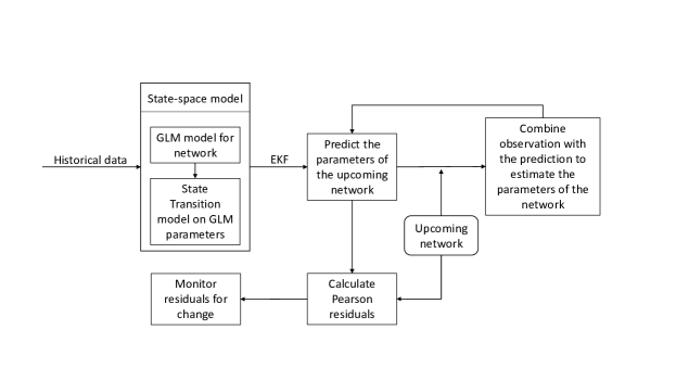
Figure 1: Overall procedure of network modeling and change detection

In this paper, we use the following notations. We denote an observed network at time $t$ with its corresponding adjacency matrix denoted by $\boldsymbol{W}_{t}=\left[w_{ij,t}\right]$, where $w_{ij,t}$ is the weight of an edge connecting nodes $i$ and $j$ at the time point $t$. In the case of binary networks, $w_{ij,t}=1$ if an edge connects nodes $i$ and $j$, and $w_{ij,t}=0$ otherwise. We denote the set of all networks up to time $t$ by $\boldsymbol{W}_{(t)}=\left\{\boldsymbol{W}_{1},\boldsymbol{W}_{2},\cdots,\boldsymbol{W}_{t}\right\}$. In general, we assume that networks are directed and there is no self-edge in the networks, i.e. $w_{ii,t}=0$ for any $i$ and $t$. Here, without loss of generality, we assume the total number of nodes remains fixed over time, and denote the number of possible edges in a network by $m=n\left(n-1\right)$, where $n$ is number of nodes. We suppose that networks are attributed and use $\boldsymbol{x}_{ij,t}$ to denote a $p$–dimensional vector of attributes corresponding to the edge between nodes $i$ and $j$ at time $t$. We let $\boldsymbol{X}_{t}=\left[\mathbf{1\;}\boldsymbol{x}_{ij,t}^{\mathtt{T}}\right]$ to denote the attribute matrix of size $m\times\left(p+1\right)$, where $\mathbf{1}$ is an $m$–dimensional vector of ones corresponding to the intercept. Note that in the case of undirected networks, $\boldsymbol{W}_{t}$ is a symmetric matrix and $\boldsymbol{x}_{ij,t}=\boldsymbol{x}_{ji,t}$. We also denote the vectorized representation of the adjacency matrix with $\boldsymbol{w}_{t}=vec\left(\left[w_{ij,t}\right]\right)$ for $i\neq j$. Here, the operator $vec\left(.\right)$ transforms the matrix $\boldsymbol{W}_{t}=\left[w_{ij,t}\right]$ into a vector of size $m$. Finally, we denote the parameters of a network that statistically relates $\boldsymbol{w}_{t}$ to $\boldsymbol{X}_{t}$ with a $p+1$ dimensional vector, $\boldsymbol{\beta}_{t}$.

Modeling of Attributed Network Streams

We begin with modeling a given attributed network $\boldsymbol{W}_{t}$ at an arbitrary time $t$ using GLM. Detailed concepts and properties of GLM can be found in (Nelder & Baker,, 1972). Given a set of attributes, we parametrize a network $\boldsymbol{W}_{t}$ by a vector of parameters $\boldsymbol{\beta}_{t}$, which transforms the network into its attribute space. This model assumes that every entry of an adjacency matrix $\boldsymbol{W}_{t}$ is an independent realization of an exponential family distribution (e.g. Bernoulli or Poisson) with parameter $\theta_{ij,t}$ given the attributes of an edge. This parameter denotes the probability of forming an edge between nodes $i$ and $j$ in a given binary network, or represents the average communication rate between two nodes in a given weighted network, at time $t$. GLM models the parameters $\theta_{ij,t}$ as a function of a linear combination of attributes, i.e., $\boldsymbol{\theta}_{t}=vec\left(\left[\theta_{ij,t}\right]\right)=g\left(\boldsymbol{X}_{t}\boldsymbol{\beta}_{t}\right)$, where $g:\mathbb{R\rightarrow\mathbb{R}}$ is an appropriate link function that depends on the type of probability distribution. Examples of link functions are $g\left(x\right)=\frac{1}{1+\exp\left(-x\right)}$ and $g\left(x\right)=e^{x}$ that can be used for modeling binary and weighted networks, receptively. To find the maximum likelihood estimate of the parameter $\boldsymbol{\beta}_{t}$ and its covariance matrix denoted as $\boldsymbol{P}_{t}$, one can use iteratively reweighted least square (IRWLS) algorithm (Nelder & Baker,, 1972) provided in the Appendix.

The static attributed network model estimates the network parameter $\boldsymbol{\beta}_{t}$, through GLM, for a given adjacency matrix and a set of attributes at time $t$. However, this approach does not consider the information of previously observed network snapshots, and consequently cannot capture network dynamics in the network stream $\boldsymbol{W}_{(t)}$. To address this issue, we integrate GLM with SSM that incorporates the information of prior networks for a more accurate estimation of model parameters. Specifically, we consider $\boldsymbol{\beta}_{t}$ as the state of the system that generates noisy observations through an observation equation given by

$$\begin{cases}w_{ij,t}\sim f\left(\theta_{ij,t}\right)\\ \boldsymbol{\theta}_{t}=vec\left(\left[\theta_{ij,t}\right]\right)=g\left(\boldsymbol{X}_{t}\boldsymbol{\beta}_{t}\right)\end{cases},$$ (1)

where $f\left(\theta_{ij,t}\right)$ denotes the probability density function of an exponential family distribution with parameter $\theta_{ij,t}$. The observation equation connects the parameters of the exponential family distribution to the network attributes and facilitates transforming the network to its attribute space. To complete the SSM, we consider the following linear state transition equation:

$$\boldsymbol{\beta}_{t}=\boldsymbol{F}\boldsymbol{\beta}_{t-1}+\boldsymbol{\xi}+\boldsymbol{\epsilon}_{t},$$ (2)

where $\boldsymbol{F}$ is the state transition matrix, $\boldsymbol{\xi}$ is a vector of constants that determines the mean value of the parameter $\boldsymbol{\beta}_{t}$, and $\boldsymbol{\epsilon}_{t}$ is the white noise assumed to follow a Gaussian distribution with mean zero and covariance matrix $\boldsymbol{Q}_{t}$. The transition matrix $\boldsymbol{F}$ is assumed either to be known, or to be estimated using system identification techniques (Ljung,, 1998). To estimate the model parameters $\boldsymbol{\beta}_{t}$, an inference procedure is required. If the SSM were linear, the Kalman filter (KF) procedure could achieve the optimal estimate of the states in terms of the least square error (Kalman,, 1960). However, clearly the observation model in (1) is nonlinear. Therefore, we employ the EKF shown to be effective in incorporating nonlinearity in parameter estimation (Fahrmeir & Kaufmann,, 1991). Similar to KF, EKF provides a recursive estimation procedure that only uses the current network snapshot (at time $t$) and the previous parameter estimates (at time $t-1$) to update the parameter estimates at time $t$. This significantly reduces the computation burden and avoids the out–of–memory issue as the network stream grows large. In the following sub-sections, we first describe the EKF approach, and then we present an approximate but simpler alternative estimation procedure based on the KF framework that replaces the nonlinear observation equation with a linear one.

Dynamic Estimation via Extended Kalman Filter

Let $\boldsymbol{\beta}_{t|t-1}$ be the Kalman prediction of $\boldsymbol{\beta}_{t}$ given all the previous observations $\boldsymbol{W}_{\left(t-1\right)}$, and let $\boldsymbol{\beta}_{t|t}$ be the Kalman estimation of $\boldsymbol{\beta}_{t}$ given all the observations up to time $t$, i.e., $\boldsymbol{W}_{\left(t\right)}$. Similarly, let $\boldsymbol{P}_{t|t-1}$ and $\boldsymbol{P}_{t|t}$ denote Kalman prediction and estimation of the covariance matrix of coefficients, $\boldsymbol{P}_{t}$. The EKF linearizes the observation equation about the predicted state $\boldsymbol{\beta}_{t|t-1}$, using the Taylor expansion to achieve a sub–optimal estimate of the state value. Let $\boldsymbol{G}_{t}$ denotes the Jacobian of $g$ evaluated at $\boldsymbol{\beta}_{t|t-1}$. This matrix is a $\left(p+1\right)\times m$ matrix obtained by $\boldsymbol{G}_{t}=\left.\frac{\partial g}{\partial\boldsymbol{\beta}_{t}}\right|_{\boldsymbol{\beta}_{t|t-1}}$. Thus, the EKF prediction equations of the state $\boldsymbol{\beta}_{t}$ and its covariance matrix $\boldsymbol{P}_{t}$ for the SSM given in (1) and (2) can be written as follows (Fahrmeir & Kaufmann,, 1991):

$$\boldsymbol{\beta}_{t|t-1}=\boldsymbol{F}\boldsymbol{\beta}_{t-1|t-1}+\boldsymbol{\xi},$$ (3)

$$\boldsymbol{P}_{t|t-1}=\boldsymbol{F}\boldsymbol{P}_{t-1|t-1}\boldsymbol{F}^{\mathtt{T}}+\boldsymbol{Q}_{t}.$$ (4)

The prediction of the observation at time $t$, i.e., $\boldsymbol{w}_{t|t-1}$, is given by the observation equation,

$$\boldsymbol{w}_{t|t-1}=g\left(\boldsymbol{X}_{t}\boldsymbol{\beta}_{t|t-1}\right),$$ (5)

and consequently Kalman estimates are obtained by

$$\boldsymbol{\beta}_{t|t}=\boldsymbol{\beta}_{t|t-1}+\boldsymbol{K}_{t}\left(\boldsymbol{w}_{t}-\boldsymbol{w}_{t|t-1}\right),$$ (6)

$$\boldsymbol{P}_{t|t}=\left(\boldsymbol{I}-\boldsymbol{K}_{t}\boldsymbol{G}_{t}\right)\boldsymbol{P}_{t|t-1},$$

where $\boldsymbol{K}_{t}$ is the Kalman gain given by $\boldsymbol{K}_{t}=\boldsymbol{P}_{t|t-1}\boldsymbol{G}_{t}\left(\boldsymbol{G}_{t}^{\mathtt{T}}\boldsymbol{P}_{t|t-1}\boldsymbol{G}_{t}+\boldsymbol{R}_{t}\right)^{-1}$. Here, $\boldsymbol{R}_{t}$ is an $m\times m$ diagonal matrix, which represents the variance of observations and is estimated based on the underlying network distribution and the observation prediction $\boldsymbol{w}_{t|t-1}$. The estimated parameter $\boldsymbol{\beta}_{t|t}$ provides a sub–optimal estimate of the network parameters at time $t$ given a sequence of networks $\boldsymbol{W}_{\left(t\right)}$ (Fahrmeir & Kaufmann,, 1991). As examples, the detailed information and equations of the estimation procedure for binary and weighted networks are given in subsequent sections.

Binary Networks

Consider a binary network at an arbitrary time $t$, i.e., $\boldsymbol{W}_{t}$. The binary network can be parametrized by a set of parameters $\theta_{ij,t}$ that denotes the probability of forming an edge between nodes $i$ and $j$. Thus, given two nodes, each element of the adjacency matrix $\boldsymbol{W}_{t}$ is a realization of a Bernoulli distribution with parameter $\theta_{ij,t}$, i.e., $w_{ij,t}\sim\textrm{Bernoulli}\left(\theta_{ij,t}\right)$. Let the logistic function $g\left(x\right)=\frac{1}{1+\exp\left(-x\right)}$ be the appropriate link function related to the Bernoulli distribution. Then, the ML estimate of the parameter $\boldsymbol{\beta}_{t}$ is achieved by maximizing the following log-likelihood function using the IRWLS given in the appendix:

$$l\left(\boldsymbol{\beta}_{t},\boldsymbol{X}_{t};\boldsymbol{w}_{t}\right)=\boldsymbol{w}_{t}^{\mathtt{T}}\log\left(\textrm{div}\left(\boldsymbol{1},\boldsymbol{1}+\exp\left(-\boldsymbol{X}_{t}\boldsymbol{\beta}_{t}\right)\right)\right)+\left(\boldsymbol{1}-\boldsymbol{w}_{t}\right)^{\mathtt{T}}\log\left(\textrm{div}\left(\exp\left(-\boldsymbol{X}_{t}\boldsymbol{\beta}_{t}\right),\boldsymbol{1}+\exp\left(-\boldsymbol{X}_{t}\boldsymbol{\beta}_{t}\right)\right)\right),$$

where $\mathbf{1}$ is a vector of size $m$ whose elements are $1$, $\textrm{div}\left(\boldsymbol{x},\boldsymbol{y}\right)$ is the element by element division of vectors $\boldsymbol{x}$ and $\boldsymbol{y}$, and the functions $\log\left(.\right)$ and $\exp\left(.\right)$ operate element–wise on the input vectors. Now, assuming the parameter $\boldsymbol{\beta}_{t}$ follows the state transition equation given in (2), the Jacobian matrix $G_{t}$ is computed by

$$\boldsymbol{G}_{t}=\left.\frac{\partial}{\partial\boldsymbol{\beta}_{t}}\left(\textrm{div}\left(\boldsymbol{1},\boldsymbol{1}+\exp\left(-\boldsymbol{X}_{t}\boldsymbol{\beta}_{t}\right)\right)\right)\right|_{\boldsymbol{\beta}_{t|t-1}}=\boldsymbol{X}_{t}^{\mathtt{T}}\textrm{diag}\left(\exp\left(-\boldsymbol{X}_{t}\boldsymbol{\beta}_{t|t-1}\right)\right)\left(\textrm{diag}\left(\mathbf{1}+\exp\left(-\boldsymbol{X}_{t}\boldsymbol{\beta}_{t|t-1}\right)\right)\right)^{-2},$$

where, $\textrm{diag}(\mathbf{x})$ is a diagonal matrix whose diagonal elements are the elements of a vector $\mathbf{x}$. The estimation of the network parameters $\beta_{t}$ is then achieved through the equation (6). The covariance matrix of observations $\boldsymbol{R}_{t}$ is an $m\times m$ diagonal matrix whose diagonal element is obtained by $\left[r_{uu,t}\right]=w_{u,t|t-1}\left(1-w_{u,t|t-1}\right)$, where $w_{u,t|t-1}$ refers to the $u^{th}$ element of the prediction vector $\boldsymbol{w}_{t|t-1}$ computed in (5).

Weighted Networks

Consider a weighted network at an arbitrary time $t$, i.e., $\boldsymbol{W}_{t}$, in which weights represent the number of communications between two nodes. This network is parametrized by a set of parameters $\theta_{ij,t}$, denoting the communication rate between two nodes $i$ and $j$. Specifically, we assume given two nodes, each element of the adjacency matrix $\boldsymbol{W}_{t}$ is a realization of a Poisson distribution with parameter $\theta_{ij,t}$, i.e., $w_{ij,t}\sim\textrm{Poisson}\left(\theta_{ij,t}\right)$. Let $g\left(x\right)=e^{x}$ be the link function related to the Poisson distribution. Then, the ML estimate of the parameter $\boldsymbol{\beta}_{t}$ is achieved by maximizing the following log-likelihood function using the IRWLS given in the appendix:

$$l\left(\boldsymbol{\beta}_{t},\boldsymbol{X}_{t};\boldsymbol{w}_{t}\right)=\boldsymbol{w}_{t}^{\mathtt{T}}\exp\left(-\boldsymbol{X}_{t}\boldsymbol{\beta}_{t}\right)-\mathbf{1^{\mathtt{T}}}\exp\left(-\boldsymbol{X}_{t}\boldsymbol{\beta}_{t}\right),$$

where $\mathbf{1}$ is a vector of size $m$ whose elements are 1. Now, suppose that the parameter $\boldsymbol{\beta}_{t}$ follows a linear state transition equation (2), then $\boldsymbol{G}_{t}$ is given by

$$\boldsymbol{G}_{t} =\left.\frac{\partial}{\partial\boldsymbol{\beta}_{t}}\left(\exp\left(-\boldsymbol{X}_{t}\boldsymbol{\beta}_{t}\right)\right)\right|_{\boldsymbol{\beta}_{t|t-1}}=\boldsymbol{X}_{t}^{\mathtt{T}}\textrm{diag}\left(\exp\left(\boldsymbol{X}_{t}\boldsymbol{\beta}_{t|t-1}\right)\right).$$

Given $\boldsymbol{G}_{t}$, the estimation of the network parameters $\boldsymbol{\beta}_{t}$ is achieved through equation (6). The covariance matrix of observations $\boldsymbol{R}_{t}$ is an $m\times m$ diagonal matrix with diagonal elements $\left[r_{uu,t}\right]=w_{u,t|t-1}$, where $w_{u,t|t-1}$ refers to the $u^{th}$ element of the prediction vector $w_{t|t-1}$ computed in (5).

Approximate Estimation via Kalman Filter

When the size of a network (adjacency matrix) is large, one may consider replacing the nonlinear observation equation with a linear equation with respect to $\boldsymbol{\beta}_{t}$. This linearization can significantly simplify the inference procedure. Let denote the static ML estimate of a network parameter at time $t$ by $\hat{\boldsymbol{\beta}_{t}}$. It is known that $\hat{\boldsymbol{\beta}_{t}}$ asymptotically follows a Gaussian distribution with mean $\boldsymbol{\beta}_{t}$ and the covariance matrix $\boldsymbol{P}_{t}$ (Myers et al.,, 2012). Therefore, as the link function for the Gaussian distribution is linear, one can rewrite the observation equation in a linear form as $\hat{\boldsymbol{\beta}_{t}}=\boldsymbol{\beta}_{t}+\boldsymbol{v}_{t}$ where $\boldsymbol{v}_{t}$ is a random $\left(p+1\right)$–vector of a zero–mean Gaussian distribution with the covariance matrix of $\boldsymbol{R}_{t}$ . Consequently, the SSM becomes linear as follows:

$$\begin{cases}\boldsymbol{\beta}_{t}=\boldsymbol{F}\boldsymbol{\beta}_{t-1}+\boldsymbol{\xi}+\boldsymbol{\epsilon}_{t},\\ \hat{\boldsymbol{\beta}_{t}}=\boldsymbol{\beta}_{t}+\boldsymbol{v}_{t}.\end{cases}$$ (7)

With the linear observation model, KF can be used to predict and estimate the parameters $\boldsymbol{\beta}_{t}$ by the following recursive equations:

$$\boldsymbol{\beta}_{t|t}=\boldsymbol{\beta}_{t|t-1}+\boldsymbol{K}_{t}\left(\hat{\boldsymbol{\beta}_{t}}-\boldsymbol{\beta}_{t|t-1}\right),$$ (8)

$$\boldsymbol{K}_{t}=\boldsymbol{P}_{t|t-1}\left(\boldsymbol{P}_{t|t-1}+\boldsymbol{R}_{t}\right)^{-1},$$ (9)

$$\boldsymbol{P}_{t|t}=\left(\boldsymbol{I}-\boldsymbol{K}_{t}\right)\boldsymbol{P}_{t|t-1},$$ (10)

where $\boldsymbol{\beta}_{t|t-1}$ and $\boldsymbol{P}_{t|t-1}$ are obtained by (3) and (4).

Monitoring of Dynamic Network Streams

Our proposed modeling approach provides a means for estimating and updating the parameters of a dynamic attributed network stream. That is, it can capture the network dynamics and the autocorrelation structure among the network snapshots. This section proposes a monitoring procedure for detecting abrupt changes in a stream of attributed networks caused by a shock different from the underlying dynamic mechanism of the network stream. In this paper, we focus on Phase II monitoring where we assume that the in-control model and its initial parameters $\boldsymbol{F}$, $\boldsymbol{\xi}$, etc., are either known or can be estimated from an in-control sequence of attributed networks denoted by $\boldsymbol{W}_{\left(T\right)}=\left\{\boldsymbol{W}_{1},\boldsymbol{W}_{2},\cdots,\boldsymbol{W}_{T}\right\}$. For each incoming network snapshot, the network parameters are predicted using the EKF or KF equations discussed before. Then, the vector of updated parameters $\boldsymbol{\beta}_{t+1|t}$ is used to predict the adjacency matrix at time $t$ for $t=T+1,...$, using the appropriate link function, i.e., $\boldsymbol{w}_{t+1|t}=g\left(\boldsymbol{X}_{t}\boldsymbol{\beta}_{t+1|t}\right)$, where $\boldsymbol{w}_{t+1|t}$ is the vectorized version of the corresponding adjacency matrix $W_{t+1|t}$ and is of size $m$. Next, the vector of Pearson residuals of size $m$ denoted by $\boldsymbol{r}_{t+1}$ is computed by (Myers et al.,, 2012)

$$r_{i,t+1}=\frac{w_{i,t+1}-w_{i,t+1|t}}{\sqrt{var\left(w_{i,t+1|t}\right)}};\>\mathrm{for}\>t=T,T+1,...,$$

where, $w_{i,t+1}$ is the the $i^{th}$ element of vectorized version of the adjacency matrix observed at time $t+1$, $w_{i,t+1|t}$ is the $i^{th}$ element of vectorized version of predicted adjacency matrix, and $r_{i,t+1}$ is the $i^{th}$ element of the residual vector $\boldsymbol{r}_{t+1}$. The prediction variance $var\left(w_{i,t+1|t}\right)$ depends on the distribution of the edge formation in the network. For example, in the case of binary network the variance is given by $var\left(w_{i,t+1|t}\right)=w_{i,t+1|t}\left(1-w_{i,t+1|t}\right)$, and in the case of weighted networks, it is given by $var\left(w_{i,t+1|t}\right)=w_{i,t+1|t}$.

If the process is in-control, Pearson residuals, $r_{i,t+1}$, asymptotically and independently follow a standard normal distribution. Therefore, one can construct an EWMA control chart to test the hypothesis whether $E(r_{i,t+1})=0$ for $t=T,T+1,...$ and $i=1,2,\cdots,m$. However, instead of monitoring each $r_{i,t+1}$, we monitor $\bar{r}_{t+1}=\frac{1}{m}{\textstyle\sum_{i=1}^{m}}r_{i,t+1}$ that also follows a normal distribution with mean zero, in the case of in-control data. The EWMA statistic at time $t+1$ is computed by $z_{t+1}=\lambda\bar{r}_{t+1}+\left(1-\lambda\right)z_{t}$, where $\lambda$ is the weight factor, and $z_{0}=0.$ The upper control limit (UCL) and the lower control limit (LCL) of the EWMA control chart at time $t$ are given by

$$UCL_{t}=l\times s\sqrt{\frac{\lambda}{1-\lambda}\left(1-\left(1-\lambda\right)^{2t}\right)},$$

$$LCL_{t}=-l\times s\sqrt{\frac{\lambda}{1-\lambda}\left(1-\left(1-\lambda\right)^{2t}\right)},$$

where $s$ is the in–control standard deviation of $\bar{r}_{t}$ and should be estimated based on the reference set $\boldsymbol{W}_{\left(T\right)}$, and $l$ and $\lambda$ are obtained through Monte Carlo simulations so that a desired in–control average run length (ARL) is achieved as detailed in the next section. If $z_{T+1}\geq UCL_{T+1}$ or $z_{T+1}\leq LCL_{T+1}$, we reject the null hypothesis, indicating a change has occurred in the network stream.

Performance Evaluation Using Simulation

This section evaluates the performance of the proposed methodology in detecting abrupt changes by using simulated streams of networks. We compare the performance of the proposed method with two benchmark approaches. The first benchmark is the static GLM that at each sampling time fits a GLM using only the current network data. In this setting, we consider the current network estimate as a prediction for the next network snapshot to calculate residuals. The second benchmark is a variant method for handling network dynamics proposed by Azarnoush et al., (2016). They suggested to aggregate the last $l_{w}$ observed networks in order to predict the upcoming network. The predicted values from each method are then used for calculating the Pearson residuals. The out–of–control average and standard deviation of run lengths are considered as performance measures for comparison.

For this simulation study, we consider a stream of communication networks of college students. Each network snapshot contains the communication information of $50$ students during a week. The age of students ranging from $20$ to $40$ is one of the two attributes used in this simulation, and is denoted by $a$. We assume that in an in-control situation the number of contacts between two students $i$ and $j$ depends on their age difference $a_{ij}=|a_{i}-a_{j}|$. That is, two students with smaller age difference are more likely to contact each other. Furthermore, we suppose five students are members of an association that holds cultural events and requests the active members to promote the events. Therefore, when the association members are active, they have an excessive communication with their network members. The association membership is modeled by a binary variable $c_{ij}$, and is considered as the second attribute. This attribute is one if its corresponding edge is adjacent to an association member, and is zero otherwise. Therefore, the vector of edge attributes denoted by $\boldsymbol{x}_{ij}=[a_{ij};c_{ij}]$, consists of a continuous and a binary variable.

We generate two types of networks: First, we consider binary networks in which an edge between two nodes at week $t$ represents at least one contact between two students during that week. Second, we simulate weighted networks, in which the weight of an edge encodes the number of times two students contacted during a particular week. For simulating a binary graph, we assume the probability of an edge between two nodes is given by the following logistic function $\theta_{ij,t}=\frac{1}{1+\exp\left(-\boldsymbol{\beta}_{t}^{\mathtt{T}}\left[1;\boldsymbol{x}_{ij}\right]\right)}.$ In the case of weighed networks, we suppose that weights follow a Poisson distribution, in which the average number of contacts is given by an exponential function as follows: $\theta_{ij,t}=\exp\left(\boldsymbol{\beta}_{t}^{\mathtt{T}}\left[1;\boldsymbol{x}_{ij}\right]\right)$. Here, $\boldsymbol{\beta}_{t}^{\mathtt{T}}=\left[\beta_{1,t}\,\,\beta_{2,t}\,\,\beta_{3,t}\right]$ is the vector of the model parameters, where $\beta_{1,t}$ is an intercept, and $\beta_{2,t}$ and $\beta_{3,t}$ represent the effect of $a_{ij,t}$ and $c_{ij,t}$ on the probability (or weight), respectively. The underlying dynamic of the communication network stream is generated through a state transition model given by $\boldsymbol{\beta}_{t}=\boldsymbol{F}\boldsymbol{\beta}_{t-1}+\boldsymbol{\xi}+\boldsymbol{\epsilon}_{t}$. In the simulations, we use $\boldsymbol{\beta}_{0}^{\mathtt{T}}=\left[-1\,\,0.05\,\,0\right]$ as initial state values, and $\boldsymbol{F}=0.7\boldsymbol{I}_{3\times 3}$, $\boldsymbol{\xi}^{\mathtt{T}}=\left[-0.6\,\,0.03\,\,0\right]$ as the parameters of the state transition model. Furthermore, we assume $\boldsymbol{\epsilon}_{t}\sim NID\left(0,\boldsymbol{Q}\right)$, where $\boldsymbol{Q}$ is a $3\times 3$ diagonal matrix with $Q_{11}=0.01$, $Q_{22}=0.0001$, $Q_{33}=0.05$. We set the initial value of $\beta_{3,t}$ to zero, indicating that the association members are inactive at the time. To generate a sequence of networks, we first generate a sequence of state values $\left\{\boldsymbol{\beta}_{t}\right\}_{t=1}^{100}$ through the state transition equation with initial values of $\boldsymbol{\beta}_{0}$. Then, a sequence of edge formation rates $\left\{\theta_{ij,t}\right\}$ is calculated through the corresponding link functions. When simulating a binary network, we generate a random number from a Bernoulli distribution with the calculated parameters $\theta_{ij,t}$ and place an edge between two nodes if the generated value is equal to one. In the case of weighted networks, we produce weights through a Poisson distribution with mean $\theta_{ij,t}$. The generated sequence of networks is considered as an input to the proposed methodology.

To evaluate the performance of the proposed methodology for each network type, we consider two scenarios where a change is imposed at time $t=\tau$ by increasing or decreasing the value of $\beta_{i,\tau}$ by $\delta\sigma_{i}$, where $\delta$ is a constant representing the magnitude of the change and $\sigma_{i}$ denotes the standard deviation of the parameter $\beta_{i}$ prior to the change given by $\sigma_{i}=\sqrt{\frac{Q_{ii}}{\left(1-F_{ii}\right)^{2}}}$. The two scenarios are as follows:

Scenario 1: We assume at time $\tau=50$, students are graduating and therefore the overall communication level is reduced. We model this change by reducing the second parameter of the transition equation by $\delta\sigma_{2}$. That is $\beta_{2,\tau}=F_{22}\beta_{2,\tau-1}+\xi_{2}+\epsilon_{2,\tau}-\delta\sigma_{2}$. This scenario represents a global change affecting all nodes.

Scenario 2: We suppose at time $\tau=50$, the student members of the association decide to become active. We model this change by increasing $\beta_{3}$ by $\delta\sigma_{3}$, i.e., $\beta_{3,\tau}=F_{33}\beta_{3,\tau-1}+\xi_{3}+\epsilon_{3,\tau}+\delta\sigma_{3}$. This scenario represents a local change, in which only few of the nodes have excessive communications with the entire network.

The control limits are calculated using the Monte–Carlo simulations to achieve the in–control ARL ($ARL_{0}$ ) of $200$. These values are obtained through $2000$ replications of the simulation and the in–control sequence of $5000$ networks. First, a network sequence of length 5000 is generated based on the in–control model. This stream is used as a reference set to estimate the standard deviation of the Pearson residuals, $s$. Then, we generate 2000 in–control network sequences of length 5000 and determine the ARL for a given pair of $l$ and $\lambda$. We repeat this procedure for several pairs of $l$ and $\lambda$ to find those resulting in $ARL_{0}$ of $200$. The resulting $l$ and $\lambda$ values for each method are reported in Table 1. We use these parameters to identify the control limits for change detection. For illustration, we plot the EWMA charts shown in the Figure 2. This figure gives an example of detection performance of each method in different scenarios. The charts illustrate the EWMA values calculated based on the Pearson residuals.

Table 1: Values of $l$ and $\lambda$ that achieves $ARL_{0}=200$

$\left(l,\lambda\right)$	Static model	Sliding static model	Dynamic model
Binary	$\left(1.79,0.3\right)$	$\left(3.33,0.1\right)$	$\left(2.44,0.1\right)$
Weighted	$\left(2.00,0.3\right)$	$\left(3.61,0.1\right)$	$\left(2.53,0.1\right)$

Binary network
Scenario 1	Scenario 2
Weighted network
Scenario 1	Scenario 2

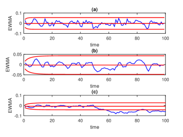
(a)

(b)

(c)

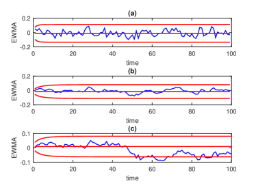
(d)

Figure 2: Plot of EWMA statistics versus time. Shift of magnitude $\delta=2$ imposed at $\tau=50$. In each figure, (a), (b), and (c) represents static model, sliding static model with $l_{w}=5$, and the dynamic model.

To compare the performance of the proposed method with the benchmarks that ignore the dynamic evolution of networks, we compute the out–of–control ARL ($ARL_{1}$) for each scenario using 2000 simulation replications. Figure 3 along with Table 2 report the performance of the proposed and benchmark methods for each network type and scenario. As it can be seen from the Figure, our proposed method that considers the dynamic evolution of the network can detect smaller changes (i.e. $\delta<2.5$) faster (with smaller standard error) than both benchmark methods in all the cases. For example, in Scenario 1, the $ARL_{1}\,\left(SERL\right)$ values of our dynamic method for detecting a change with the magnitude of $\delta=1.5$ in binary network streams is 8.57 (0.144), while these values for the static and sliding static methods are, respectively, 113.27 (3.869) and 59.32 (2.770). This indicates that the dynamic method can detect such a change around 15 and 9 times faster than the benchmark methods.

The main reason that benchmark methods fail to detect small changes is that these methods do not properly capture autocorrelation structure among the network snapshots (i.e. gradual changes) caused by network dynamics, resulting in a small $ARL_{0}$ (or large false alarm rate). Therefore, by keeping $ARL_{0}$ close to 200, these methods lose the detection power leading to large $ARL_{1}$. Another reason for poor performance of the static method is that they have a very short window of opportunity for detecting a change. In the static method, we predict the next network only based on the current network estimations. If a change appears upon the arrival of the next network (i.e. new regime starts) the difference between the arriving network and its prediction is larger than the previous cases, representing a change. However, if this change is not detected at the change point, the prediction of the future networks are made based on the estimation of the networks that are already generated based on the new regime and therefore the residuals become small. This short window of opportunity in detection of changes is also reflected in the standard errors of the benchmark methods, reported in Table 2. The large standard error values indicate that a change is either detected very quickly or never been detected by the benchmarks. For larger changes (i.e. $\delta\geq 2.5$) the performance of all three methods are comparable, though the proposed method still has slightly smaller detection delay in the case of binary networks.

For the local change in binary networks (Scenario 2), the excessive communication cannot be completely captured, due to the limited data. This limitation is reflected in the detection power of all three methods. That is, all three methods have larger $ARL_{1}$ values compared with the corresponding global changes. Nevertheless, the dynamic method significantly outperforms the benchmarks in detecting a local change in binary networks. This again shows the importance of capturing the network dynamics and its effect in change detection. When we model the communication considering the number of contacts (weighted networks), the local change is more apparent and can be detected by all three methods when it is large enough. However, our proposed method can still detect smaller local changes faster in weighted network streams.

Binary network
Scenario 1 (a)	Scenario 2 (b)
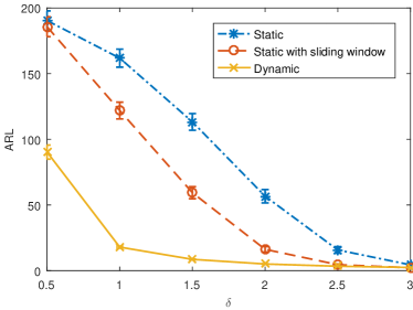
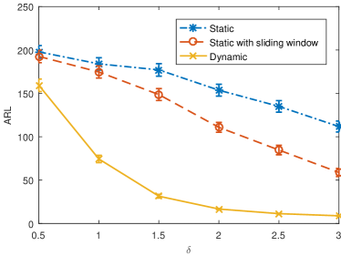
Weighted network
Scenario 1 (c)	Scenario 2 (d)

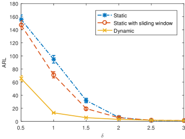
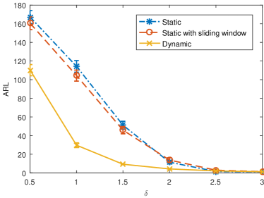
Figure 3: Average run length as a function of change magnitude for the proposed modeling framework and the benchmarks

Table 2: Standard error ($\frac{\sigma_{ARL_{1}}}{\sqrt{n}}$ for $n=2000$) as a function of change magnitude for the proposed modeling framework and the benchmarks

Binary network
Scenario 1	Scenario 2
$\delta$ Static Sliding static Dynamic $0.5$ 4.494 4.617 3.270 $1$ 4.156 3.874 0.486 $1.5$ 3.869 2.770 0.144 $2$ 3.096 1.260 0.083 $2.5$ 1.520 0.319 0.051 $3$ 0.785 0.053 0.036	$\delta$ Static Sliding static Dynamic $0.5$ 4.406 4.416 4.387 $1$ 4.319 4.256 2.580 $1.5$ 4.391 4.161 1.298 $2$ 4.171 3.444 0.403 $2.5$ 4.053 3.298 0.189 $3$ 3.828 2.821 0.145
Weighted network
Scenario 1	Scenario 2
$\delta$ Static model Sliding static Dynamic $0.5$ 4.184 3.954 2.633 $1$ 3.543 2.860 0.257 $1.5$ 2.110 1.262 0.109 $2$ 0.735 0.828 0.057 $2.5$ 0.056 0.027 0.031 $3$ 0.020 0.019 0.014	$\delta$ Static Sliding static Dynamic $0.5$ 4.273 4.154 3.653 $1$ 3.878 3.613 1.544 $1.5$ 2.577 2.366 0.178 $2$ 1.122 1.496 0.090 $2.5$ 0.103 0.543 0.042 $3$ 0.020 0.024 0.016

1 Case Study: Enron’s Dynamic Email Network

In this section, to show how our proposed method can be applied to real problems, we model and monitor the Enron email communication network. The Enron corpus consist of about 0.5 millions of email communications among $184$ employees of the Enron corporation from 1998 to 2002 (Priebe et al.,, 2005). This dataset can be represented by a sequence of directed networks, where each network represents one week of email communications. A directed edge is placed between nodes $i$ and $j$ at time $t$ if at least one email has been sent from employee $i$ to the employee $j$ during week $t$. The role of each employee within the company is available and used to set the attributes of networks. The roles consist of CEO, president, vice–president, manager, director, trader, and employee. For simplicity, we focus on the emails sent among president (P), mangers and directors (MR), and CEO. The combination of these roles result in a categorical attribute for each edge with nine possible values (i.e. CEO-CEO, CEO–P, CEO–MR, …), which are represented by dummy variables. Note that in these networks, given the attributes (employee roles), the existence of an edge between two nodes is independent from the existence of other edges.

First, we aggregate 30 initial weeks of data into a single network and estimate the initial value of the network parameters using the static method. We select first 30 weeks due to small number of emails available during that period. We also set $F$ to be identity matrix and $\xi$ to be zero, which mimics a random walk process. The dynamic model with EKF is used to infer the parameters of each graph. The estimated parameters were used to calculate the Pearson residuals and to detect changes in the stream of networks. We use data from week 31 to 60 as an in-control stream to estimate the standard deviation of Pearson residuals used to calculate the control limits. Figure 4 illustrates the EWMA chart of the Pearson residuals obtained from the proposed dynamic model. As can be seen, the EWMA chart signals between week 79 and 89. These out-of-control signals relate to the time period that Enron scandal was revealed (Azarnoush et al.,, 2016).

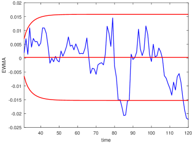
Figure 4: EWMA chart of the Pearson residuals obtained from the proposed dynamic model. The chart signals between week 79 and 89 that matches the time of a major event in Enron history

To further explore the change and its potential causes, we calculate the probability of an edge between two nodes with particular roles. Because of the few exchanged emails during the first 30 weeks, we do not include those weeks in the results. Figure 5a illustrates the communication probability of two CEOs. As shown, this probability drastically changes at weeks $76$ and $89$. This result is consistent with the observation in the study by Xu & Hero, (2014). Based on this observation, we speculate that the underlying reason behind the change is an excessive communication among the CEOs. We setup another EWMA chart, shown in Figure 5b, based on the Pearson residual of sub-networks whose nodes represent the CEOs. As it is illustrated, the control chart detects both jumps in the CEOs communication. These jumps relate to the CEO resignation at the Enron Corporation because of the famous scandal.

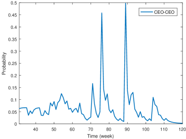
(a)

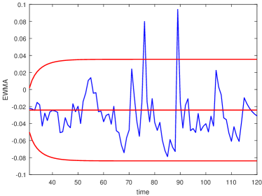
(b)

Figure 5: Analysis of Enron data (a) Estimated probability of communication between two CEOs (b) Change detection using Pearson residuals of the CEO–CEO sub–graphs.

2 Conclusion

In this paper, we proposed a new methodology for modeling and monitoring of attributed network streams. First, we modeled static networks using GLM. Next, we introduced a state transition model over the network parameters to capture its dynamics. Using the EKF, we predicted network parameters used for calculating the Pearson residuals (i.e. the standardized residuals between the predicted and observed networks). Pearson residuals were then monitored by using EWMA control charts for quick detection of abrupt changes. We examined the proposed method using both simulated and real data. In the simulation study, we generated a stream of attributed networks representing interactions among college students both in the form of binary and weighted networks. We considered two change scenarios for each type of the networks, one modeling a global change and one representing a local change in the stream of networks. The proposed method was compared with two benchmarks, which fail to fully capture the network dynamics. The results showed that the proposed method’s detection delay is significantly smaller than two benchmarks, particularly when the change magnitude is small. Furthermore, the performance of all three methods deteriorated when detecting local changes in binary networks. This was due to the lack of data in capturing the excessive communications. However, the dynamic method still outperformed both of the benchmarks in detection of local changes. Finally, we used the Enron corpus as a case study. Our method detected the excessive communication of the CEO’s related to the time period that Enron scandal was revealed. The results of the case study agree with other studies on the Enron data. In recent years, several authors proposed different techniques for community detection in networks. A potential future research direction is to combine the community detection techniques with the proposed methodology to detect changes in the community structures over time.

Appendix: Iteratively Reweighted Least Square Method

Assume that observations $w_{ij,t}$, denoting the weight of the edge between nodes $i$ and $j$ at time $t$, come from a distribution in exponential family distribution. That is, $w_{ij,t}\sim f\left(w_{ij,t};\theta_{ij,t}\right)$ with

$$f\left(w_{ij,t};\theta_{ij,t}\right)=\exp\left\{\frac{w_{ij,t}\theta_{ij,t}-b\left(\theta_{ij,t}\right)}{a\left(\phi_{ij,t}\right)}+c\left(w_{ij,t},\phi_{ij,t}\right)\right\}.$$

Here, $\theta_{ij,t}$ and $\phi_{ij,t}$ are canonical and dispersion parameters respectively, and $a\left(.\right)$, $b\left(.\right)$, and $c\left(.\right)$ are known function related to the particular distribution. We assume $a\left(\phi_{ij,t}\right)=\frac{\phi_{ij,t}}{p}$, which holds for most of the distributions in the exponential family including the Bernoulli and Poisson distributions. The constant $p$ is assumed to be known a priori. Now, assume $\theta_{ij,t}=g\left(\left[1,b_{ij}\right]^{\mathtt{T}}\boldsymbol{\beta}_{t}\right)$ where, $g\left(.\right)$ is the link function and $\boldsymbol{x}_{ij}$ is the attribute vector of an edge between nodes $i$ and $j$.

Given a network with the adjacency matrix $\left[w_{ij,t}\right]$, and attributes $\boldsymbol{x}_{ij}$, the goal of IRWLS is to estimate the parameter $\boldsymbol{\beta}_{t}$ by maximizing the log–likelihood function

$$l\left(w_{ij,t};\theta_{ij,t}\right)=\sum_{i=1}^{n}\sum_{j=1}^{n}\frac{w_{ij,t}\theta_{ij,t}-b\left(\theta_{ij,t}\right)}{a\left(\phi\right)}+c\left(w_{ij,t},\phi\right)$$

The IRWLS algorithm works as follows: Given a trial estimate of $\hat{\boldsymbol{\beta}_{t}}$, one calculates $\eta_{ij,t}=\left[1,\boldsymbol{x}_{ij}\right]^{\mathtt{T}}\hat{\boldsymbol{\beta}_{t}}$, and $\hat{\theta}_{ij,t}=g\left(\left[1,\boldsymbol{x}_{ij}\right]^{\mathtt{T}}\hat{\boldsymbol{\beta}_{t}}\right)$. These quantities are used in calculation of working dependent variable $z_{ij,t}=\hat{\eta}_{ij,t}+\left(w_{ij,t}-\hat{\theta}_{ij,t}\right)\frac{d\eta_{ij,t}}{d\theta_{ij,t}}$, and the iterative weights $q_{ij,t}=\frac{p}{\left(\frac{\partial^{2}b}{\partial\theta_{ij,t}^{2}}\right)\left(\frac{d\eta_{ij,t}}{d\theta_{ij,t}}\right)^{2}}$, where all the derivatives are evaluated at the trial estimate. Given the working dependent variable and the weights, one can re–estimate the $\boldsymbol{\beta}_{t}$ using the weighted least square formulation as

$$\hat{\boldsymbol{\beta}_{t}}=\left(\boldsymbol{X}^{\mathtt{T}}\boldsymbol{Q}_{t}\boldsymbol{X}\right)^{-1}\boldsymbol{X}^{\mathtt{T}}\boldsymbol{Q}_{t}\boldsymbol{z}_{t},$$

where $\boldsymbol{X}$ is the matrix of the attributes, $\boldsymbol{Q}_{t}$ is a diagonal matrix with diagonal elements $q_{ij,t}$, and $\boldsymbol{z}_{t}$ is a vector with elements $z_{i}$. This procedure can simply be done using the Matla$b^{\circledR}$ function glmfit from the Statistics and Machine Learning Toolbo$x^{\left(TM\right)}$.

References

- Aggarwal et al., (2011) Aggarwal, Charu C, Zhao, Yuchen, & Yu, Philip S. 2011. Outlier detection in graph streams. Pages 399–409 of: Data engineering (icde), 2011 ieee 27th international conference on. IEEE.
- Azarnoush et al., (2016) Azarnoush, Bahareh, Paynabar, Kamran, Bekki, Jennifer, & Runger, George. 2016. Monitoring temporal homogeneity in attributed network streams. Journal of quality technology, 48(1), 28.
- Barabási & Albert, (1999) Barabási, Albert-László, & Albert, Réka. 1999. Emergence of scaling in random networks. science, 286(5439), 509–512.
- Duan et al., (2009) Duan, Dongsheng, Li, Yuhua, Jin, Yanan, & Lu, Zhengding. 2009. Community mining on dynamic weighted directed graphs. Pages 11–18 of: Proceedings of the 1st acm international workshop on complex networks meet information & knowledge management. ACM.
- ERDdS & R&WI, (1959) ERDdS, P, & R&WI, A. 1959. On random graphs i. Publ. math. debrecen, 6, 290–297.
- Fahrmeir & Kaufmann, (1991) Fahrmeir, Ludwig, & Kaufmann, Heinz. 1991. On kalman filtering, posterior mode estimation and fisher scoring in dynamic exponential family regression. Metrika, 38(1), 37–60.
- Frank & Strauss, (1986) Frank, Ove, & Strauss, David. 1986. Markov graphs. Journal of the american statistical association, 81(395), 832–842.
- Goldenberg et al., (2010) Goldenberg, Anna, Zheng, Alice X, Fienberg, Stephen E, & Airoldi, Edoardo M. 2010. A survey of statistical network models. Foundations and trends® in machine learning, 2(2), 129–233.
- Hanneke et al., (2010) Hanneke, Steve, Fu, Wenjie, Xing, Eric P, et al. 2010. Discrete temporal models of social networks. Electronic journal of statistics, 4, 585–605.
- Hirose et al., (2009) Hirose, Shunsuke, Yamanishi, Kenji, Nakata, Takayuki, & Fujimaki, Ryohei. 2009. Network anomaly detection based on eigen equation compression. Pages 1185–1194 of: Proceedings of the 15th acm sigkdd international conference on knowledge discovery and data mining. ACM.
- Hoff et al., (2002) Hoff, Peter D, Raftery, Adrian E, & Handcock, Mark S. 2002. Latent space approaches to social network analysis. Journal of the american statistical association, 97(460), 1090–1098.
- Kalman, (1960) Kalman, Rudolph Emil. 1960. A new approach to linear filtering and prediction problems. Journal of basic engineering, 82(1), 35–45.
- Kim & Leskovec, (2012) Kim, Myunghwan, & Leskovec, Jure. 2012. Multiplicative attribute graph model of real-world networks. Internet mathematics, 8(1-2), 113–160.
- Kleinberg, (2002) Kleinberg, Jon. 2002. Small-world phenomena and the dynamics of information. Advances in neural information processing systems, 1, 431–438.
- Koutra et al., (2012) Koutra, Danai, Papalexakis, Evangelos E, & Faloutsos, Christos. 2012. Tensorsplat: Spotting latent anomalies in time. Pages 144–149 of: Informatics (pci), 2012 16th panhellenic conference on. IEEE.
- Koutra et al., (2013) Koutra, Danai, Vogelstein, Joshua T, & Faloutsos, Christos. 2013. Deltacon: A principled massive-graph similarity function. arxiv preprint arxiv:1304.4657.
- Ljung, (1998) Ljung, Lennart. 1998. System identification. Springer.
- Marchette, (2012) Marchette, David. 2012. Scan statistics on graphs. Wiley interdisciplinary reviews: Computational statistics, 4(5), 466–473.
- McCulloh, (2009) McCulloh, Ian. 2009. Detecting changes in a dynamic social network. ProQuest.
- McCulloh & Carley, (2011) McCulloh, Ian, & Carley, Kathleen M. 2011. Detecting change in longitudinal social networks. Tech. rept. DTIC Document.
- Myers et al., (2012) Myers, Raymond H, Montgomery, Douglas C, Vining, G Geoffrey, & Robinson, Timothy J. 2012. Generalized linear models: with applications in engineering and the sciences. Vol. 791. John Wiley & Sons.
- Neil et al., (2013) Neil, Joshua, Hash, Curtis, Brugh, Alexander, Fisk, Mike, & Storlie, Curtis B. 2013. Scan statistics for the online detection of locally anomalous subgraphs. Technometrics, 55(4), 403–414.
- Nelder & Baker, (1972) Nelder, John A, & Baker, RJ. 1972. Generalized linear models. Encyclopedia of statistical sciences.
- Papadimitriou et al., (2010) Papadimitriou, Panagiotis, Dasdan, Ali, & Garcia-Molina, Hector. 2010. Web graph similarity for anomaly detection. Journal of internet services and applications, 1(1), 19–30.
- Perry et al., (2013) Perry, Marcus B, Michaelson, Gregory V, & Ballard, M Alan. 2013. On the statistical detection of clusters in undirected networks. Computational statistics & data analysis, 68, 170–189.
- Priebe et al., (2005) Priebe, Carey E, Conroy, John M, Marchette, David J, & Park, Youngser. 2005. Scan statistics on enron graphs. Computational & mathematical organization theory, 11(3), 229–247.
- Ranshous et al., (2015) Ranshous, Stephen, Shen, Shitian, Koutra, Danai, Harenberg, Steve, Faloutsos, Christos, & Samatova, Nagiza F. 2015. Anomaly detection in dynamic networks: a survey. Wiley interdisciplinary reviews: Computational statistics, 7(3), 223–247.
- Sarkar & Moore, (2005) Sarkar, Purnamrita, & Moore, Andrew W. 2005. Dynamic social network analysis using latent space models. Acm sigkdd explorations newsletter, 7(2), 31–40.
- Sparks & Ickowicz, (2013) Sparks, Ross, & Ickowicz, Adrien. 2013. Spatio-temporal disease surveillance: Forward selection scan statistic. arxiv preprint arxiv:1309.7721.
- Sun et al., (2006a) Sun, Jimeng, Tao, Dacheng, & Faloutsos, Christos. 2006a. Beyond streams and graphs: dynamic tensor analysis. Pages 374–383 of: Proceedings of the 12th acm sigkdd international conference on knowledge discovery and data mining. ACM.
- Sun et al., (2006b) Sun, Jimeng, Papadimitriou, Spiros, & Philip, S Yu. 2006b. Window-based tensor analysis on high-dimensional and multi-aspect streams. Pages 1076–1080 of: Icdm, vol. 6.
- Wang et al., (2012) Wang, Shanshan, Wu, Teresa, Weng, Shao-Jen, & Fowler, John. 2012. A control chart based approach to monitoring supply network dynamics using kalman filtering. International journal of production research, 50(11), 3137–3151.
- Watts & Strogatz, (1998) Watts, Duncan J, & Strogatz, Steven H. 1998. Collective dynamics of small-world networks. nature, 393(6684), 440–442.
- Woodall et al., (2016) Woodall, William H, Zhao, Meng J, Paynabar, Kamran, Sparks, Ross, & Wilson, James D. 2016. An overview and perspective on social network monitoring. arxiv preprint arxiv:1603.09453.
- Xu & Hero, (2014) Xu, Kevin S, & Hero, Alfred O. 2014. Dynamic stochastic blockmodels for time-evolving social networks. Selected topics in signal processing, ieee journal of, 8(4), 552–562.