2$\alpha$+$t$ cluster structure in ${{}^{11}{\rm B}}$

Abstract

The 2$\alpha+t$ cluster structure in ¹¹B is investigated by the microscopic generator coordinate method (GCM) with the Brink cluster wave functions. With a proper choice of the parameters of the effective interaction, the calculated energy spectrum shows reasonable agreement with the observed low-lying spectra of both parities. On the basis of the calculated radii, monopole and $B(E2)$ transition strengths, several developed cluster states of ¹¹B are suggested. For the negative-parity states, in addition to the well-known $3/2_{3}^{-}$ cluster state, the $1/2_{2}^{-}$ and $5/2_{3}^{-}$ states are also proposed as the well-developed cluster states. For the positive-parity states, it is found that many states around the 2$\alpha+t$ threshold show the feature of developed clusters. In particular, the $1/2_{2}^{+}$ state is found to have a linear-chain-like structure, which is consistent with the previous antisymmetrized molecular dynamics calculation, but contradicts to the orthogonality condition model calculation. It is also found that many of these positive-parity cluster candidates have the non-negligible isoscalar dipole transition strengths, which require the experimental confirmation.

I Introduction

The study of cluster states of light nuclei Wildermuth and Tang (1977); Fujiwara et al. (1980); Kanada-En’yo et al. (2003); Freer (2007); Horiuchi et al. (2012); Kimura et al. (2016) has always been an important subject in nuclear physics, which provides us with a new perspective for understanding nuclear structure and many-body problem in atomic nuclei. The ${{}^{12}{\rm C}}$ is one of the most typical clustered nuclei. In particular, its famous Hoyle state is known as an $\alpha$ condensed state Tohsaki et al. (2001, 2017) or gas-like state. This kind of well-developed cluster states shows us a novel motion of clusters in a nucleus, which cannot be explained by the single-particle picture. In this decade, the search for the gas-like or well-developed cluster states von Oertzen et al. (2006); Itoh et al. (2011); Yang et al. (2014); He et al. (2014); Zhou et al. (2016); Baba and Kimura (2016) in self-conjugate $n\alpha$ nuclei and also in non-$n\alpha$ nuclei attract great interest both in experiment and theory.

In analogy to the 3$\alpha$ cluster structure in ${{}^{12}{\rm C}}$, it is a very interesting subject to investigate the developed 2$\alpha+t$ cluster structure around the threshold energy in the non-self-conjugate nucleus ${{}^{11}{\rm B}}$. In particular, it is the central interest in this study if we can find the gas-like cluster state analog to the Hoyle state in ${}^{12}{\rm C}$. The early orthogonality condition model (OCM) calculation by Nishioka et al. Nishioka et al. (1979) showed that the $3/2^{-}_{3}$ state at 8.56 MeV and the several negative-parity states around 10 MeV are the promising candidates for the well-developed $2\alpha+t$ clustering, while the low-lying states are the compact shell-model-like states. They also concluded that the positive-parity states have the transient nature between the shell and cluster structure in ${{}^{11}{\rm B}}$.

Decades later, the antisymmetrized molecular dynamics (AMD) calculations showed that Suhara and Kanada-En’yo (2012) the $3/2^{-}_{3}$ state has the prominent $2\alpha+t$ cluster structure without any a-priori assumption on the cluster formation. They also showed that Suhara and Kanada-En’yo (2012) the $3/2^{-}_{3}$ state has the strong IS monopole transition strength from the ground state because of its spatially extended cluster structure whose matter radius is 2.65 fm. This enhancement of the IS monopole transition strength is in good accordance with the observation Kawabata et al. (2007a). On the basis of the analysis using the Brink wave function, they showed that Kanada-En’yo and Suhara (2015) the $t$ cluster has broad spatial distribution around the $2\alpha$ cluster core, which is the reason why they concluded the $3/2^{-}_{3}$ state as the Hoyle analog state.

More recently, Yamada et al. Yamada and Funaki (2010) renewed the Nishioka’s work by performing the OCM calculation with much larger model space. They confirmed that the $3/2_{3}^{-}$ state has a $2\alpha+t$ cluster structure with a large matter radius of 3.00 fm. Furthermore, they reported that the $1/2_{2}^{+}$ state at 12.56 MeV has a dilute cluster structure with a very large nuclear radius of 6 fm. By analyzing the cluster orbits occupied by the $\alpha$ and $t$ clusters, they concluded that the $1/2_{2}^{+}$ state should be regarded as the Hoyle analog state as all clusters are approximately occupying $s$-wave states, while they are not in the $3/2^{-}_{3}$ state. Recently, by a new measurement of $\alpha$ resonant scattering on ⁷Li, Yamaguchi et al. Yamaguchi et al. (2011) did not observe the strong resonance $1/2^{+}$ state at 11.7$-$13.1 MeV, instead, they proposed the existence of another $3/2^{+}$ or $9/2^{+}$ state at 12.63 MeV. So far, the experimental counterpart for this $1/2_{2}^{+}$ state has not been identified yet.

Thus, two different Hoyle analog states, the $3/2^{-}_{3}$ and $1/2^{+}_{2}$ states, were suggested as the candidates of the Hoyle analog state by two different types of the theoretical models, AMD Suhara and Kanada-En’yo (2012); Kanada-En’yo and Suhara (2015) and OCM Yamada and Funaki (2010). The former (the $3/2^{-}_{3}$ state) is experimentally identified well by its pronounced IS monopole transition, but cannot have the $s$-wave nature because of its spin and parity. On the other hand, the $1/2^{+}_{2}$ state can have the $s$-wave nature which is the most prominent characteristics of the Hoyle state. However, its existence Yamaguchi et al. (2011) is experimentally uncertain as it may be a broad resonance and cannot be populated by the IS monopole transition from the ground state. It is also noted that no microscopic cluster models report the existence of the $1/2^{+}$ state with the $s$-wave nature, and only the semi-microscopic calculations (OCM) report it.

This contradicting and puzzling situation motivated us to conduct the study of the $2\alpha+t$ cluster states based on the microscopic cluster model. We will study the cluster states in the framework of the generator coordinate method (GCM) using the Brink wave functions as the basis wave functions. Based on the excitation energies, radii, and the transition strengths, we will discuss the possible developed cluster states in ${{}^{11}{\rm B}}$. Our main interests in this work are as follows. (1) The property of the $3/2^{-}_{3}$ state. Is it consistent with the other theories and experiments? (2) Are there other pronounced cluster states in the negative-parity states other than $3/2^{-}_{3}$ state? (3) Is there the $1/2^{+}$ state with $s$-wave nature by the microscopic model calculation? (4) What is a good experimental probe for the positive-parity cluster states ?

The paper is organized as follows. In Sec. II, we present the formulations of the GCM with 2$\alpha+t$ Brink wave functions for ${{}^{11}{\rm B}}$. Then we will show the results and make discussions in Sec. III. Finally, we present the summary in Sec. IV.

II Theoretical framework

II.1 Hamiltonian and GCM wave function

The Hamiltonian used in the present study includes the kinetic energy, effective nucleon-nucleon and Coulomb interactions,

$$H=\sum_{i=1}^{11}t_{i}-t_{\rm cm}+\sum_{i<j}^{11}v_{NN}+\sum_{i<j}^{11}v_{\rm Coul},$$ (1)

where $t_{\rm cm}$ denotes the center-of-mass kinetic energy which is exactly removed from the total energy. As the effective nucleon-nucleon interaction, we employed the Volkov No.2 interaction Volkov (1965) combined with the spin-orbit part of the G3RS interaction Yamaguchi et al. (1979); Okabe and Abe (1979) which is given as,

$$v_{NN}= \sum_{n=1}^{2}v_{n}e^{-r_{ij}^{2}/a_{n}^{2}}(W+BP_{\sigma}-HP_{\tau}-MP_{\sigma}P_{\tau})$$

$$+\sum_{n=1}^{2}w_{n}e^{-r_{ij}^{2}/b_{n}^{2}}P(^{3}O)\bm{L}\cdot\bm{S}.$$ (2)

Here $P_{\sigma}$, $P_{\tau}$, and $P(^{3}O)$ denote the spin and isospin exchange operators and the projection operator to the triplet-odd states, respectively. The parameter set is listed in Table. 1, which is slightly modified from that adopted in Ref. Suhara and Kanada-En’yo (2012) to reproduce the binding energy of the ground state and the splitting between the $3/2^{-}_{1}$ and $1/2^{-}_{1}$ states, simultaneously.

Table 1: Adopted parameter set for the Volkov No.2 interaction and the spin-orbit part of the G3RS interaction. The units of $v_{n}$ and $w_{n}$ are MeV. The units of $a_{n}$ and $b_{n}$ are fm and fm^-2, respectively

$v_{1}$	$v_{2}$	$a_{1}$	$a_{2}$	$W$	$B$	$H$	$M$
$-60.65$	$61.14$	$1.80$	1.01	0.41	0.125	0.125	0.59
$w_{1}$	$w_{2}$	$b_{1}$	$b_{2}$
$2800$	$-2800$	$0.4472$	$0.60$

In this study, we employ the Brink wave function Brink (1966) for the basis wave function of the GCM calculation. The system composed of the 2$\alpha+t$ clusters located at $\bm{R}_{1},\bm{R}_{2}$, and $\bm{R}_{3}$ is described as follows,

$$\Phi(\{R\},s) =\mathcal{A}[\Phi_{\alpha}(\mbox{\boldmath$R$}_{1})\Phi_{\alpha}(\mbox{\boldmath$R$}_{2})\Phi_{t}(\mbox{\boldmath$R$}_{3},s)],$$ (3)

$$\Phi_{\alpha}(\bm{R}) =\mathcal{A}\{\phi(\bm{R})\chi_{n\uparrow}\cdots\phi(\bm{R})\chi_{p\downarrow}\},$$ (4)

$$\Phi_{t}(\bm{R},s) =\mathcal{A}\{\phi(\bm{R})\chi_{n\uparrow}\phi(\bm{R})\chi_{n\downarrow}\phi(\bm{R})\chi_{ps}\},$$ (5)

$$\phi(\mbox{\boldmath$R$}) =\Bigl{(}\frac{1}{\pi b^{2}}\Bigr{)}^{3/4}e^{-\left(\mbox{\boldmath$r$}-\mbox{\boldmath$R$}\right)^{2}/(2b^{2})},$$ (6)

where $\Phi_{\alpha}$ and $\Phi_{t}$ denote the wave functions of $\alpha$ and $t$ clusters, respectively. $\phi(\mbox{\boldmath$R$})$ is the Gaussian wave packet for the single nucleon located at $\bm{R}$. The size parameter $b$ is chosen as $1/(2b^{2})=0.235$ fm^-2. $\chi_{p\uparrow},...,\chi_{n\downarrow}$ represent the spin-isospin wave functions, and the spin of the proton in the $t$ cluster denoted by $s$ is either of up or down. $\bm{R}_{1}$, $\bm{R}_{2},$ and $\bm{R}_{3}$ are the generator coordinates and abbreviated as $\{R\}=\{\mbox{\boldmath$R$}_{1},\mbox{\boldmath$R$}_{2},\mbox{\boldmath$R$}_{3}\}$. The condition $4\bm{R}_{1}+4\bm{R}_{2}+3\bm{R}_{3}=0$ is imposed to remove the center-of-mass motion.

By the parity and angular-momentum projections, we obtain the projected wave functions,

$$\Phi^{J\pi}_{MK}(\{R\},s)=P^{J}_{MK}(\Omega)P^{\pi}\Phi(\{R\},s),$$ (7)

where $P^{\pi}$ and $P^{J}_{MK}(\Omega)$ denote the parity and angular momentum projectors. Then the projected basis wave functions with different values of the generator coordinates $\{R\}$, $s$, and different projections of the angular momentum $K$ are superposed,

$$\Psi^{J\pi}_{M}=\sum_{\{R\}sK}g_{\{R\}sK}\Phi^{J\pi}_{MK}(\{R\},s).$$ (8)

The coefficients of the superposition $g_{\{R\}sK}$ and the eigenenergies $E$ are obtained by solving the Hill-Wheeler equation Ring and Schuck (2004),

$$\sum_{\{R^{\prime}\}s^{\prime}K^{\prime}}g_{\{R^{\prime}\}s^{\prime}K^{\prime}}\braket{\Phi^{J\pi}_{MK}(\{R\},s)}{H}{\Phi^{J\pi}_{MK^{\prime}}(\{R^{\prime}\},s^{\prime})}$$

$$=E\sum_{\{R^{\prime}\}s^{\prime}K^{\prime}}g_{\{R^{\prime}\}s^{\prime}K^{\prime}}\braket{\Phi^{J\pi}_{MK}(\{R\},s)}{\Phi^{J\pi}_{MK^{\prime}}(\{R^{\prime}\},s^{\prime})}.$$ (9)

From the GCM wave function, we can directly calculate physical quantities such as radii and the transition probabilities.

In the practical calculation, the generator coordinates $\{R\}=\{\bm{R}_{1},\bm{R}_{2},\bm{R}_{3}\}$ are chosen so that their inter-distances $R_{ij}=|\bm{R}_{i}-\bm{R}_{j}|$ range from 1 to 6 fm with an interval of 1 fm. This choice of the generator coordinate, together with the degree-of-freedom of the triton spin direction, yields 186 Brink wave functions to be used as the basis wave function of the GCM calculation. To check the stability of the obtained GCM wave functions, we also performed GCM calculations by adopting larger model spaces for comparison. For example, we increased the maximum length of the inter-distance up to 8 fm, and found that the obtained states around and below the $2\alpha+t$ threshold, which are of our interest in the present study, are almost stable. More importantly, we confirmed that the general feature of the physical quantities such as the IS monopole transitions are also stable. However, it is also noted that the highly excited states lying well above the $2\alpha+t$ threshold are sensitive to the choice of the model space because of their strong coupling with the many-body continua. This requires the application of some methods to describe broad resonances, which will be our main focus in the next work.

II.2 Isoscalar monopole, dipole, and electric quadrupole transitions

Recent years, the isoscalar monopole (ISM) transition has been regarded as a powerful probe to identify the developed cluster states, since it strongly induces clustering as proved by Yamada et al. Yamada et al. (2008, 2012). Indeed, many cluster states in light stable nuclei including the $3/2^{-}_{3}$ state of ${}^{11}{\rm B}$ are experimentally known to have enhanced ISM transition strength from the ground state. In this study, we utilize the ISM strengths from the low-lying $1/2^{+}_{1}$ and $5/2^{+}_{1}$ states to identify the clustered $1/2^{+}$ and $5/2^{+}$ states, although the direct measurement of the transition strength is not easy. The ISM operator $\mathcal{M}^{\rm ISM}$ and the reduced transition strength from the state $\ket{J_{i}M_{i}}$ to the state $\ket{J_{f}M_{f}}$ are defined as,

$$\mathcal{M}^{\rm ISM} =\sum_{i=1}^{A}(\bm{r}_{i}-\bm{r}_{\rm cm})^{2},$$ (10)

$$B(ISM;J_{i}\rightarrow J_{f}) =|\braket{J_{f}M_{f}}{\mathcal{M}^{\rm ISM}}{J_{i}M_{i}}|^{2},$$ (11)

where $\bm{r}_{i}$ and $\bm{r}_{\rm cm}$ denote the $i$th nucleon coordinate and the center-of-mass, respectively.

In addition to the ISM transition, the isoscalar dipole (ISD) transition has been proposed as an another probe Chiba et al. (2016); Kanada-En’yo (2016); Chiba et al. (2017) for the clustering. The transition operator and strength are defined as,

$$\mathcal{M}^{\rm ISD}_{\mu} =\sum_{i=1}^{A}(\bm{r}_{i}-\bm{r}_{\rm cm})^{3}Y_{1\mu}(\widehat{\bm{r}_{i}-\bm{r}_{\rm cm}}),$$ (12)

$$B(ISD;J_{i}\rightarrow J_{f}) =\sum_{M_{f}\mu}|\braket{J_{f}M_{f}}{\mathcal{M}^{\rm ISD}_{\mu}}{J_{i}M_{i}}|^{2}.$$ (13)

It is noted that the ISD excitation from the $3/2^{-}$ ground state yields the excited $1/2^{+}$, $3/2^{+}$, and $5/2^{+}$ states. We expect that the magnitude of the ISD transition strengths can be a clustering measure for these spin-parity states.

The electric quadrupole transition strength is also calculated to investigate the band structure. Its transition operator and strength are given as,

$$\mathcal{M}_{\mu}^{\rm E2}=e^{2}\sum_{i=1}^{A}(\bm{r}_{i}-\bm{r}_{\rm cm})^{2}Y_{2\mu}(\widehat{\bm{r}_{i}-\bm{r}_{\rm cm}})\frac{1-\tau_{iz}}{2},$$ (14)

$$B(E2;J_{i}\rightarrow J_{f})=\sum_{M_{f}\mu}|\braket{J_{f}M_{f}}{\mathcal{M}^{\rm E2}_{\mu}}{J_{i}M_{i}}|^{2}.$$ (15)

Here $\tau_{iz}$ is the isospin projection of the $i$th nucleon. We use the $B(E2)$ strength to assign the possible band structure of the excited states.

II.3 Overlap between GCM and projected Brink wave functions

A GCM wave function is a superposition of many projected Brink wave functions having different generator coordinates $\{R\}$, spin $s$, and different projections of the angular momentum $K$ in the body-fixed frame. Therefore, it is not straightforward to assign cluster configuration to each GCM wave function. For this purpose, it is convenient to introduce the overlap between the GCM and projected Brink wave functions. Here, the body-fixed frame and the Brink wave function used as a reference state are defined as illustrated in Fig.  1.

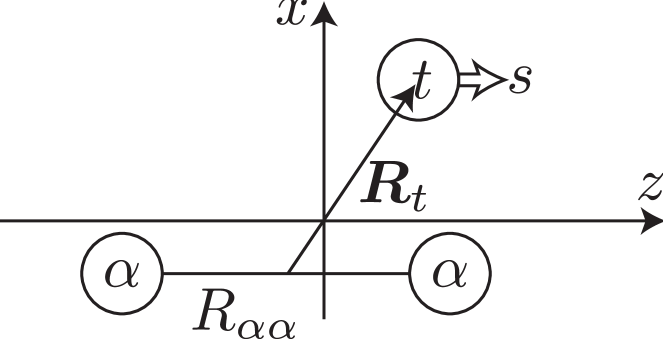
Figure 1: Schematic figure of 2$\alpha+t$ Brink wave function, which is used to define the squared overlap given by Eq. (16).

The two $\alpha$ clusters are aligned along the $z$ axis with the inter-cluster distance $R_{\alpha\alpha}$, and the $t$ cluster is located at $\bm{R}_{t}$ on the $zx$-plane. The triton spin direction is represented by $s$. With this Brink wave function denoted by $\Phi(R_{\alpha\alpha},\bm{R}_{t},s)$, the squared overlap with the GCM wave function is defined as

$$O(R_{\alpha\alpha},\bm{R}_{t}) =\sum_{sKs^{\prime}K^{\prime}}\braket{\Psi^{J\pi}_{M}}{P^{J\pi}_{MK}\Phi(R_{\alpha\alpha},\bm{R}_{t},s)}S_{sKs^{\prime}K^{\prime}}^{-1}$$

$$\times\braket{P^{J\pi}_{MK^{\prime}}\Phi(R_{\alpha\alpha},\bm{R}_{t},s^{\prime})}{\Psi^{J\pi}_{M}}.$$ (16)

Here $S_{sKs^{\prime}K^{\prime}}$ denotes the overlap between the reference Brink wave functions,

$$S_{sKs^{\prime}K^{\prime}}=\braket{P^{J\pi}_{MK}\Phi(R_{\alpha\alpha},\bm{R}_{t},s)}{P^{J\pi}_{MK^{\prime}}\Phi(R_{\alpha\alpha},\bm{R}_{t},s^{\prime})},$$ (17)

and its inverse satisfies the relationship,

$$\sum_{s^{\prime}K^{\prime}}S_{sKs^{\prime}K^{\prime}}S^{-1}_{s^{\prime}K^{\prime}s^{\prime\prime}K^{\prime\prime}}=\delta_{ss^{\prime\prime}}\delta_{KK^{\prime\prime}}.$$ (18)

We expect that the magnitude of thus-defined squared overlap is a good measure to find the 2$\alpha$ clusters with inter-cluster distance $R_{\alpha\alpha}$ and the triton cluster at the position $\bm{R}_{t}$. We will use this quantity to discuss the distribution of $t$ cluster around the 2$\alpha$ cluster core. It must be noted that $O(R_{\alpha\alpha},\bm{R}_{t})$ does not correspond to the probability, because the Brink wave functions with different cluster positions are unorthogonal to each other. In other words, the integral of the squared overlap,

$$4\pi\int dR_{\alpha\alpha}d^{3}R_{t}\ R_{\alpha\alpha}^{2}O(R_{\alpha\alpha},\bm{R}_{t}),$$ (19)

is larger than unity by its definition.

III Results and Discussions

III.1 Energy levels

Figure 2 shows the energy levels obtained by the present calculation (GCM) and they are compared with the experimental data, OCM Yamada and Funaki (2010) and AMD Suhara and Kanada-En’yo (2012) calculations. Note that, in the present calculation, the $3/2^{-}_{1}$ and $1/2^{-}_{1}$ energies are fitted to the experiment to determine the parameter set of the effective interaction, but other states are not. We see that thus-determined parameter set plausibly describes the low-lying positive- and negative-parity bound states (the states below the ${}^{7}{\rm Li}+\alpha$ threshold) and qualitatively agrees with the observation, although it does not bound the $3/2^{+}_{1}$ state in contradiction to the experiment. It is also noted that the ${}^{7}{\rm Li}+\alpha$ and $2\alpha+t$ threshold energies and the energies of the ${}^{7}{\rm Li}(3/2^{-})$ and ${}^{7}{\rm Li}(1/2^{-})$ are also reasonably described, indicating that the parameter set yields reasonable inter-cluster potential for the $\alpha+t$ system.

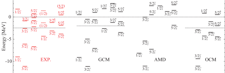
Figure 2: Comparison of obtained energy levels from GCM, AMD Suhara and Kanada-En’yo (2012), OCM Yamada and Funaki (2010) calculations and experiments Kelley et al. (2012) for the ${{}^{11}{\rm B}}$. The shown experimental and theoretical excitation energies are relative to their corresponding 2$\alpha$+$t$ threshold energies. The above and below dash lines represent the 2$\alpha$+$t$ and ⁷Li($3/2^{-}$)+$\alpha$ threshold, respectively.

In addition to the bound states, the calculation yields highly excited states around and above the threshold energies. In particular, as we will discuss in the following, the states around the $2\alpha+t$ threshold energy such as the $1/2_{2}^{-}$, $3/2_{3}^{-}$ and $1/2_{2}^{+}$ states are the candidates of the pronounced clustering. We see that these highly excited states can also be assigned to the observed states from their excitation energies.

The AMD calculation Suhara and Kanada-En’yo (2012) yields the negative-parity spectrum quite similar to ours, because a similar interaction parameter set except for much weaker spin-orbit strength ($w_{1}=-w_{2}=1600$) was employed. However, we see that it yields quite different positive-parity spectrum and no state exists below the $2\alpha+t$ threshold. The origin of the difference between the present and AMD calculations can be explained as follows. In the AMD study, the intrinsic wave functions were calculated before the angular momentum projection, which does not necessarily yield the energy minimum state after the angular momentum projection. Therefore, it can fail to describe the lowest energy states for a given spin and parity. Indeed, as we see later, the lowest $1/2^{+}$ state obtained by the AMD calculation has the linear-chain-like structure, which is similar to our $1/2^{+}_{2}$ state. On the other hand, the $1/2^{+}_{1}$ state obtained by the present calculation looks missing in the AMD result.

The OCM calculation Yamada and Funaki (2010) adopts the inter-cluster potentials which reproduce the $\alpha+\alpha$ and $\alpha+t$ systems, and introduces phenomenological three-cluster interaction to reproduce the binding energy of ${}^{11}{\rm B}$. It yields similar energy spectra to ours, and the positive-parity spectrum shows slightly better agreement with the experiment. As explained later, the structure of the $1/2^{+}$ state is quite different between the OCM and the present calculation, which may originates in the difference of the effective interaction. One should also note that the observed deepest positive-parity state is the $1/2_{1}^{+}$ state, while the OCM and present calculations fail to reproduce the correct order of the positive-parity states.

III.2 Negative-parity states in ${{}^{11}{\rm B}}$ 

III.2.1 radii and transition strengths

We begin with the ground state of ${{}^{11}{\rm B}}$ and the excited $3/2^{-}$ states, namely $J^{\pi}=3/2_{1}^{-}$, $3/2_{2}^{-}$, and $3/2_{3}^{-}$ states. These negative-parity states have been well studied by AMD, OCM, and experiments, and the comparison with these results would be useful for verifying present calculations.

Table 2: Root-mean-square (r.m.s) radii in the unit of fm for mass distribution of negative-parity states from GCM Brink, AMD Suhara and Kanada-En’yo (2012), OCM Yamada and Funaki (2010) and experiment.

State	GCM Brink	AMD	OCM	Experiment
$3/2_{1}^{-}$	2.38	2.29	2.22	2.09 $\pm$ 0.12
$3/2_{2}^{-}$	2.64	2.46	2.23
$3/2_{3}^{-}$	2.99	2.65	3.00

In Table 2, the root-mean-square (r.m.s) radii of the $3/2^{-}$ states from different cluster models and experiment are shown. For the ground state, the theoretical models, especially our GCM Brink model, overestimate the experiment. This may be due to the underestimation of the cluster distortion effect in the ground state by the cluster models. However, it is noted that the present calculation plausibly yields the electric quadrupole moment of the ground state 4.07 $e^{2}\text{fm}^{2}$, which fairly agrees with the observed value 4.07(3) $e^{2}\text{fm}^{2}$ Stone (2005). As for the excited $3/2^{-}$ states, the GCM Brink and OCM both predict larger radii than the ground state. In particular, the radius of the $3/2_{3}^{-}$ state is approximately 3.0 fm and it is comparable with that of the Hoyle state. The radius of this state from AMD is also relatively large indicating the pronounced clustering of this state.

Table 3: Calculated values of isoscalar monopole transition strengths in the unit of $\rm fm^{4}$. The corresponding results from AMD Suhara and Kanada-En’yo (2012), OCM Yamada and Funaki (2010), and experiment Kawabata et al. (2007a) are also shown for comparison.

	GCM Brink	AMD	OCM	Experiment
$3/2_{1}^{-}\to 3/2_{2}^{-}$	8.42	2.5	$-$	< 9
$3/2_{1}^{-}\to 3/2_{3}^{-}$	147	150	92	96 $\pm$ 16

As already discussed in Refs. Kawabata et al. (2007a); Yamada et al. (2008), the enhanced monopole transition strength from the ground state is a good measure of the clustering of the excited states, and the $3/2^{-}_{3}$ state is known to have fairly large transition strength. In Table 3, we compare our results of the isoscalar monopole transition strengths with those from AMD, OCM, and experiment. The observed large ISM transition strength Kawabata et al. (2007a), $B(ISM;3/2_{1}^{-}\to 3/2_{3}^{-}$)=96 $\pm$ 16 fm⁴, provides us with a strong support for the developed cluster structure of $3/2_{3}^{-}$ state. The AMD and OCM confirmed the large ISM transition strength successively. Now, in our calculations, we also obtained a quite large ISM transition strength, $B(ISM;3/2_{1}^{-}\to 3/2_{3}^{-}$)=147 fm⁴, which is consistent with the experimental data and quite close to the AMD result. We also note that the calculated ISM transition strength from the ground state to the second $3/2^{-}$ state is 8.42 fm⁴, which is also consistent with the experiment (< 9 fm⁴). From these observations, i.e. the large radius and ISM transition strength, the AMD, OCM, and the present GCM Brink reach the same conclusion; the $3/2_{3}^{-}$ state is a very developed cluster state of ${{}^{11}{\rm B}}$.

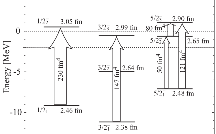
Figure 3: The GCM-Brink energy levels, r.m.s radii for the mass distributions (right side of the energy levels), and the isoscalar monopole transition strengths (stronger than 30 fm⁴) for the negative-parity states in ${{}^{11}{\rm B}}$. The above and below dash lines are corresponding to the 2$\alpha$+$t$ threshold energy and ⁷Li($3/2^{-}$)+$t$ threshold energy, respectively. Units for the energy and radius are MeV and fm, respectively.

Besides the well-confirmed $3/2_{3}^{-}$ cluster state, there also exist several $1/2^{-}$ and $5/2^{-}$ states around the 2$\alpha+t$ or ${}^{7}{\rm Li}+t$ threshold energies, which are also the candidates of the developed cluster states. We expect that the ISM transitions from the low-lying $1/2^{-}$ and $5/2^{-}$ states serve as a measure of the clustering. Figure 3 summarizes the calculated energies, r.m.s radii and ISM transition strengths of the $1/2^{-}$ and $5/2^{-}$ states together with those for the $3/2^{-}$ states. Firstly, it is noted that the radii of the low-lying $1/2^{-}_{1}$ and $5/2^{-}_{1}$ states are as small as the ground state indicating their compact shell-model nature as already pointed out by Nishioka et al. Nishioka et al. (1979). Compared to these compact states, the $1/2^{-}$ and $5/2^{-}$ states around the $2\alpha+t$ threshold have larger radii comparable with or larger than the $3/2^{-}_{3}$ state indicating their dilute clustering. Moreover, it must be noted that the ISM transition strengths to these dilute states are considerably enhanced. Although it is difficult to directly measure these quantities, we consider that they are important signature of the cluster development. Thus, the present result suggests that $1/2^{-}_{2}$ and $5/2^{-}_{3}$ states also have dilute cluster structure.

Table 4: Comparison of the $B(E2)$ strengths of negative-parity states between the GCM Brink, AMD Kawabata et al. (2007b); Suhara and Kanada-En’yo (2012) calculations and the observation Kelley et al. (2012). The unit is $e^{2}\rm fm^{4}$.

Transition	GCM Brink	AMD	Experiment
$1/2_{1}^{-}\to 3/2_{1}^{-}$	4.80	4.6	5.2 $\pm$ 0.8
$1/2_{1}^{-}\to 3/2_{2}^{-}$	15.5	13.4	$116_{-26}^{+233}$
$3/2_{1}^{-}\to 3/2_{2}^{-}$	0.07	0.02	$0.83_{-0.51}^{+0.71}$
$3/2_{1}^{-}\to 3/2_{3}^{-}$	1.5	0.84	$-$
$3/2_{1}^{-}\to 5/2_{1}^{-}$	14.3	13.8	13.3 $\pm$ 4.8
$3/2_{1}^{-}\to 5/2_{2}^{-}$	2.7	0.6	$\leq$ 0.02
$5/2_{1}^{-}\to 5/2_{2}^{-}$	1.6	$-$	0.49 $\pm$ 0.39

We next discuss the $B(E2)$ transition strengths which are useful to test the accuracy of the present calculation and to identify possible band structure. In Table 4, several $B(E2)$ transition strengths between low-lying states are listed to compare the theoretical results with the observations. Basically, the present GCM Brink results are qualitatively consistent with the AMD results. Namely, the transitions $3/2^{-}_{1}\to 5/2^{-}_{1}$ and $1/2^{-}_{1}\to 3/2^{-}_{2}$ are enhanced, while others are not. This characteristics reasonably agrees with the observation indicating that the present calculation is reliable.

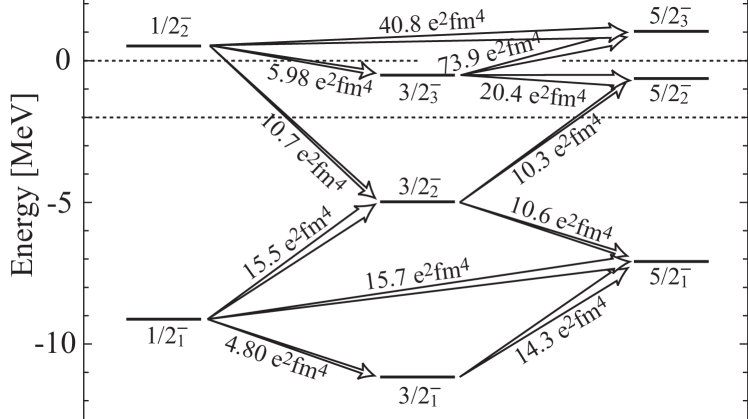
Figure 4: Calculated $B(E2)$ transition strengths between the negative-parity states in ${{}^{11}{\rm B}}$. The transition strengths lower than 4.80 $e^{2}\rm fm^{4}$ are not shown.

Then, we discuss the possible band structure from the systematics of the $B(E2)$ strengths summarized in Fig. 4. There are several points to be noted in this figure. Firstly, the transition strength $1/2^{-}_{1}\to 3/2^{-}_{2}$ is strong, while that for $1/2^{-}_{1}\to 3/2^{-}_{1}$ is not. This is because the $1/2^{-}_{1}$ and $3/2^{-}_{2}$ states are dominated by the $K^{\pi}=1/2^{-}$ component, while the $3/2^{-}_{2}$ state is dominated by the $K^{\pi}=3/2^{-}$ component. On the other hand, the $5/2^{-}$ states are the admixture of the $K^{\pi}=3/2^{-}$ and $1/2^{-}$ components. This explains, for example, why the $5/2^{-}_{1}$ state has strong transitions from all of the $1/2^{-}_{1}$, $3/2^{-}_{1}$ and $3/2^{-}_{2}$ states. Despite of the $K^{\pi}=3/2^{-}$ and $5/2^{-}$ admixture in the $5/2^{-}$ states, we suggest a $K^{\pi}=3/2^{-}$ band composed of the $3/2^{-}_{1}$ and $5/2_{1}^{-}$ states, and a $K^{\pi}=1/2^{-}$ band composed of the $1/2^{-}_{1}$ , $3/2^{-}_{2}$ and $5/2^{-}_{2}$ states.

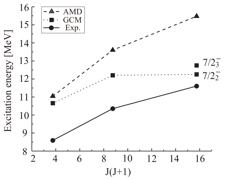
Figure 5: Comparison of the calculated $K^{\pi}=3/2^{-}$ bands with GCM Brink ($3/2^{-}_{3}$, $5/2^{-}_{3}$, and $7/2^{-}_{2}$), AMD ($3/2^{-}_{3}$, $5/2^{-}_{3}$, and $7/2^{-}_{3}$), and the experimental band ($3/2^{-}_{3}$, $5/2^{-}_{3}$, and $7/2^{-}_{3}$) suggested in Ref. Yamaguchi et al. (2011).

Secondly, we see that the $1/2_{2}^{-}$, $3/2_{3}^{-}$, and $5/2_{3}^{-}$ states, which we classified as the pronounced cluster states, have large transition strengths because of their large radii. It can be seen that the transition $1/2_{2}^{-}\to 3/2^{-}_{3}$ is rather weak, while $1/2_{2}^{-}\to 5/2^{-}_{3}$ is strong. Again, it is explained by the $K^{\pi}=3/2^{-}$ dominance in the $3/2^{-}_{2}$ state, and the $K^{\pi}=1/2^{-},\ 3/2^{-}$ admixture in the $5/2^{-}$ states.

Furthermore, it is found that the transition $3/2_{3}^{-}\to 5/2_{3}^{-}$ is considerably enhanced. The AMD calculation also found the significantly large transition between $3/2_{3}^{-}$ and $5/2_{3}^{-}$ states (and also the $7/2_{3}^{-}$ and $9/2_{3}^{-}$ states), and hence they suggested a possible band formation built on the $3/2^{-}_{3}$ state as shown in Fig. 5. In the present calculation, we find two possible candidates of the $7/2^{-}$ states which can be assinged as the band member state. The $7/2^{-}_{2}$ and $7/2^{-}_{3}$ are located at 12.25 and 12.75 MeV, respectively. Their $E2$ transition strengths from the $5/2^{-}_{3}$ state are 26.6 and 5.8 $e^{2}\rm fm^{4}$, and those from the $3/2^{-}_{3}$ state are 18.3 and 23.4 $e^{2}\rm fm^{4}$. However, because of the coupling with the continuum, present results for $7/2^{-}$ states are somewhat ambiguous. Experimentally, by the resonant scattering, a possible candidate for this rotational band was reported by Yamaguchi et al. Yamaguchi et al. (2011).

Finally, we note that the compact shell-model states ($1/2^{-}_{1}$, $3/2^{-}_{1}$ and $5/2^{-}_{1}$ states) and the dilute cluster states ($1/2^{-}_{2}$, $3/2^{-}_{3}$, and $5/2^{-}_{3}$ states) are disconnected by the $E2$ transitions due to their considerably different structure. We also note that the $3/2^{-}_{2}$ and $5/2^{-}_{2}$ states have strong transition with both of the compact shell-model and dilute cluster states. This may be because of their transient character between shell and cluster as seen in their intermediate radius sizes.

III.2.2 distribution of $t$ cluster

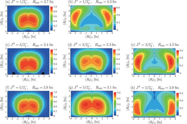
Figure 6: Contour plots of the squared overlap $O(R_{\alpha\alpha},\bm{R}_{t})$ defined by Eq. (16) for the $J^{\pi}=1/2^{-}$, $3/2^{-}$, and $5/2^{-}$ states as a function of $\bm{R}_{t}$. The horizontal axis corresponds to the $z$ component of $\bm{R}_{t}$, while the vertical axis corresponds to the $x$ component. The optimum distance between 2$\alpha$ clusters which maximizes the squared overlap is also shown.

To study the cluster configuration in the negative-parity states, the squared overlap ${O}(R_{\alpha\alpha},\bm{R}_{t})$ defined by Eq. (16) was calculated. The distance between 2$\alpha$ clusters $R_{\alpha\alpha}$ is chosen to be an optimum value so that the squared overlap is maximized with the proper choice of $\bm{R}_{t}$. Thus, by fixing the $R_{\alpha\alpha}$, the contour plots of $O(R_{\alpha\alpha},\bm{R}_{t})$ are shown in Fig. 6, which show how the $t$ cluster is distributed around the 2$\alpha$ clusters in ${{}^{11}{\rm B}}$.

Figure 6 clearly shows that the optimum values of $R_{\alpha\alpha}$ for the low-lying states ($1/2_{1}^{-}$, $3/2_{1}^{-}$, and $5/2_{1}^{-}$) are smaller than those of the high-lying cluster states. In these low-lying states, we also see that the distribution of the $t$ cluster is confined to a rather small region reflecting the compact shell-model structure. For example, in case of the ground state, the squared overlap has the maximum value of ${O}(R_{\alpha\alpha},\bm{R}_{t})=0.93$ with $R_{\alpha\alpha}=2.4$ fm and $|\bm{R}_{t}|=2.2$ fm. This means that the ground state can be reasonably approximated by a single Brink wave function with small inter-cluster distance.

The high-lying cluster states ($1/2_{2}^{-}$, $3/2_{3}^{-}$, and $5/2_{3}^{-}$) show quite contrasting characteristics. Firstly, they all have relatively large optimum $R_{\alpha\alpha}$, which are larger than 4 fm. Moreover, the $t$ cluster has a wider distribution. For example, in the case of the gas-like cluster state $3/2_{3}^{-}$, the squared overlap has the maximum value of $O(R_{\alpha\alpha},\bm{R}_{t})=0.57$ with $R_{\alpha\alpha}=4.2$ fm and $|\bm{R}_{t}|=4.0$ fm. The smaller value of the maximum overlap and larger value of the inter-cluster distance indicate that the state cannot be approximated by a single cluster configuration due to its dilute gas-like nature. It must be noted that the $1/2^{-}_{2}$ and $5/2_{3}^{-}$ states also show quite similar distributions, and hence, we conclude that they also have dilute cluster structure.

As a whole for the negative-parity states, with the increase of excitation energy, we see that the compact shell-model states evolve to the developed cluster states. The $3/2_{2}^{-}$ and $5/2_{2}^{-}$ can be regarded as the intermediate states, which have larger $R_{\alpha\alpha}$ and wider $t$-cluster distributions than the ground state.

III.3 Positive-parity states in ${{}^{11}{\rm B}}$ 

III.3.1 radii and transition strengths

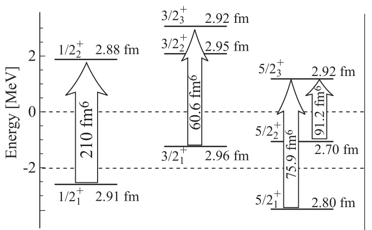
Figure 7: The GCM-Brink energy levels, r.m.s radii for the mass distributions (right side of the energy levels), and the isoscalar monopole transition strengths (stronger than 60 fm⁴) for the positive-parity states in ${{}^{11}{\rm B}}$. The above and below dash lines are corresponding to the 2$\alpha$+$t$ threshold energy and ⁷Li($3/2^{-}$)+$t$ threshold energy, respectively. The Units for the energy and radius are MeV and fm, respectively.

In general, compared with the negative-parity states, the calculated positive-parity states are located at relatively high energy region, and are all around the 2$\alpha+t$ or ${}^{7}{\rm Li}(3/2^{-})+t$ threshold energies. Therefore, it seems that more positive-parity states are promising to have developed cluster structure.

Table 5: The r.m.s radii for mass distributions of $1/2^{+}$ states from GCM Brink and OCM calculations Yamada and Funaki (2012). The unit is fm.

State	GCM Brink	OCM
$1/2_{1}^{+}$	2.91	2.82
$1/2_{2}^{+}$	2.88	5.93

Similar to the nagative-parity case, we expect that the well-developed positive-parity cluster states should also have pronounced monopole transition strengths from the $1/2^{+}_{1}$, $3/2^{+}_{1}$, and $5/2^{+}_{1}$ states. Figure 7 shows the calculated energy levels, r.m.s radii, and the ISM transition strengths for the positive-parity states. For the $J^{\pi}=1/2^{+}$ states, a very strong ISM transition strength between $1/2^{+}_{1}$ and $1/2^{+}_{2}$ states was obtained, which reaches 210 fm⁴ and even much stronger than the ISM strength between the ground and $3/2^{-}_{3}$ states. The strong ISM transitions also occur between the $3/2^{+}_{1}$ state and $3/2^{+}_{3}$ state, and between the $5/2^{+}_{1}$ state and $5/2^{+}_{3}$ state. Indeed, from the view of radius, except for the $5/2^{+}_{2}$ state, all the other states have very large radii comparable with that of the developed $3/2^{-}_{3}$ cluster state, which indicate that these most positive-parity states can be considered as the candidates of cluster states in ${{}^{11}{\rm B}}$.

In the OCM calculation, the obtained $1/2^{+}_{2}$ state is a strong candidate for the Hoyle-analogue state in which all clusters occupy the dilute $s$-wave state. An important feature for this state obtained by the OCM study is its extremely large radius, 5.93 fm. However, in the present calculation, the radius of the $1/2^{+}_{2}$ state is not so large and even smaller than that of the $1/2^{+}_{1}$ state, which can be seen in Table 5. This means that the $1/2^{+}_{2}$ states obtained by the GCM Brink and OCM are incompatible, which will be discussed later.

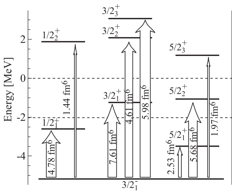
Figure 8: ISD transitions from the ground state to the positive-parity states in ${{}^{11}{\rm B}}$.

Besides the ISM transition, the ISD transition is another useful probe for the clustering. Since most of the calculated positive-parity states have large radii, we expect that the isoscalar dipole transition can be enhanced. Unexpectedly, the obtained ISD transition strengths are not enhanced as shown in Fig. 8. The calculated transition strengths range from 1.4 to 7.6 fm⁶, which are not as strong as the single-particle estimate 21.6 $\rm fm^{6}$. These strengths should be directly compared with the experimental data to test the wave functions of the present calculation. There must be some kind of underlying theoretical reason for these relatively weak but distinct strengths, which will be explored in the future.

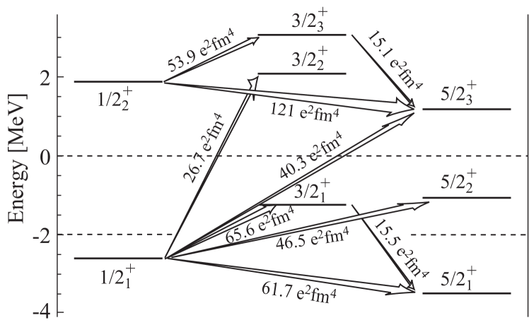
Figure 9: Positive-parity energy levels with the $B(E2)$ transition strengths (stronger than 15 $e^{2}$fm⁴).

Next, we focus on the $B(E2)$ transition strengths shown in Fig. 9. Clearly, the excited states are classified into two groups; ($1/2^{+}_{1}$, $3/2^{+}_{1}$, $5/2^{+}_{1}$) and ($1/2^{+}_{2}$, $3/2^{+}_{3}$, $5/2^{+}_{3}$), which are mutually connected with strong transitions. These two groups of states show quite similar pattern. For example, the strengths $B(E2;1/2^{+}_{1}\to 3/2^{+}_{1})$ and $B(E2;1/2^{+}_{2}\to 3/2^{+}_{3})$ are both quite strong and larger than 50 $e^{2}\rm fm^{4}$ while the strengths $B(E2;3/2^{+}_{1}\to 5/2^{+}_{1})$ and $B(E2;3/2^{+}_{3}\to 5/2^{+}_{3})$ are about 15 $e^{2}\rm fm^{4}$. The $3/2^{+}_{2}$ state is admixture of the $K^{\pi}=1/2^{+}$ and $3/2^{+}$ components, which explains the non-negligible transition strength between $1/2^{+}_{1}$ and $3/2^{+}_{2}$ states. Another fact to be reminded is, as we already mentioned, that there are also very strong monopole transitions between the corresponding states.

III.3.2 distribution of $t$ cluster

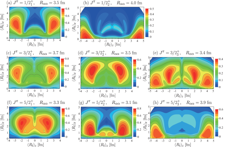
Figure 10: Contour plots of the squared overlap $O(R_{\alpha\alpha},\bm{R}_{t})$ defined by Eq. (16) for the $J^{\pi}=1/2^{+}$, $3/2^{+}$, and $5/2^{+}$ states as a function of $\bm{R}_{t}$. The horizontal axis corresponds to the $z$ component of $\bm{R}_{t}$, while the vertical axis corresponds to the $x$ component. The optimum distance between 2$\alpha$ clusters which maximizes the squared overlap is also shown.

Figure 10 is the contour plot of the squared overlap between the Brink wave function and GCM wave function for the positive-parity states. Overall, most of the positive-parity states show the pronounced clustering as expected, in which the optimum 2$\alpha$ distance $R_{\alpha\alpha}$ is very large and the triton cluster has relatively broad distribution. We see that there are several different patterns in the $t$ cluster distributions.

First and most obviously, the obtained $1/2^{+}_{2}$ state has a linear-chain structure. In Fig 10 (b), it can be seen that the squared overlap is largest at each end of the $z$ axis ($(R_{t})_{x}=0$ and $|(R_{t})_{z}|=4.3$ fm), but rapidly decreases in other region. This indicates that the $t$ cluster is mostly confined in the linearly aligned $\alpha$-$\alpha$-$t$ or $t$-$\alpha$-$\alpha$ configuration. The squared overlap has a maximum value 0.476 when $R_{\alpha\alpha}=4.0$ fm and $|\bm{R}_{t}|=4.3$ fm, which approximately corresponds to touching three clusters. This explains why the r.m.s radius of the $1/2^{+}_{2}$ state is not so large and even smaller than that of the $1/2^{+}_{1}$ state. It is noted that the $1/2^{+}_{1}$ state obtained by the AMD calculation Suhara and Kanada-En’yo (2012) has quite similar linear-chain structure. The reported excitation energy 13.6 MeV is also very close to the present result 13.0 MeV. Therefore, we may be able to conclude that our $1/2^{+}_{2}$ state and the $1/2^{+}_{1}$ state reported by AMD calculation are identical state. The reason for the missing $1/2^{+}$ state in the AMD calculation corresponding to our $1/2^{+}_{1}$ state may be due to the calculation procedure applied in the AMD study. They performed the energy variation before the angular momentum projection, which occasionally fails to describe the energetically unfavored states.

In contrast to the AMD result, the OCM calculation reported no linear-chain configurations, but reported the dilute gas-like charactor of the $1/2^{+}_{2}$ state. Therefore, it is a quite interesting and important problem to clarify the character of the $1/2^{+}_{2}$ state.

Moreover, in addition to the $1/2^{+}_{2}$ state, the $5/2^{+}_{3}$ state also shows a kind of bent linear-chain structure, e.g., the maximum square overlap 0.54 appears at $(R_{t})_{x}=0.8$ fm and $|(R_{t})_{z}|=3.9$ fm. In fact, we have mentioned that these two states have been strongly connected by $E2$ transition and the strength $B(E2;1/2^{+}_{2}\to 5/2^{+}_{3})$ is as high as 121 $e^{2}$fm⁴. In Fig. 10, from the distributions of triton cluster, it can be seen that the isosceles triangle shape is not favored for the cluster states in ${{}^{11}{\rm B}}$. In addition, the $5/2^{+}_{1}$ state is shown having a compact cluster structure, considering it is the lowest positive-parity state in our calculations and it has a relatively small radius, which can be considered as a transient state in ${{}^{11}{\rm B}}$.

IV Summary

In this study, we investigated cluster states in ${{}^{11}{\rm B}}$ using the GCM Brink wave functions. Firstly, with a proper choice of the parameters of the effective interaction, the energy spectrum including the negative-parity and positive-parity states were reproduced in the present framework. Moreover, based on the calculated radii and monopole transition strengths, several cluster states around the 2$\alpha$+$t$ threshold energy were suggested in ${{}^{11}{\rm B}}$. Some rotational bands were also discussed according to the obtained $B(E2)$ transition strengths. Furthermore, by calculating the squared overlap between GCM Brink and projected Brink wave functions, the $t$-cluster distributions were shown for different states and the proposed cluster states were further supported.

For negative-parity states in ${{}^{11}{\rm B}}$, the $1/2_{2}^{-}$ and $5/2_{3}^{-}$ states as well as the well-known $3/2_{3}^{-}$ state were shown to be the well-developed cluster states. The obtained $3/2_{3}^{-}$ and $5/2_{3}^{-}$ states were strongly connected by $E2$ transitions and a rotational cluster band $K^{\pi}$=$3/2^{-}$ was proposed. In the description of the negative-parity states of ${{}^{11}{\rm B}}$, GCM Brink, AMD, and OCM actually are quite consistent and they provide us with similar results from the comparisons. As for the positive-parity states, most states around 2$\alpha$+$t$ threshold show some features of cluster structure. Most importantly, it is found that the obtained $1/2_{2}^{+}$ state can be considered as a linear-chain-like state, which is consistent with the $1/2_{1}^{+}$ state from AMD but very different from the obtained $1/2_{2}^{+}$ state from OCM. To clarify further the characters of positive-parity cluster states especially the $1/2_{2}^{+}$ cluster state, the experimental data for the isoscalar dipole transition strengths were highly required.