Message Passing Stein Variational Gradient Descent

Abstract

Stein variational gradient descent (SVGD) is a recently proposed particle-based Bayesian inference method, which has attracted a lot of interest due to its remarkable approximation ability and particle efficiency compared to traditional variational inference and Markov Chain Monte Carlo methods. However, we observed that particles of SVGD tend to collapse to modes of the target distribution, and this particle degeneracy phenomenon becomes more severe with higher dimensions. Our theoretical analysis finds out that there exists a negative correlation between the dimensionality and the repulsive force of SVGD which should be blamed for this phenomenon. We propose Message Passing SVGD (MP-SVGD) to solve this problem. By leveraging the conditional independence structure of probabilistic graphical models (PGMs), MP-SVGD converts the original high-dimensional global inference problem into a set of local ones over the Markov blanket with lower dimensions. Experimental results show its advantages of preventing vanishing repulsive force in high-dimensional space over SVGD, and its particle efficiency and approximation flexibility over other inference methods on graphical models.

1 Introduction

Stein variational gradient descent (SVGD) (Liu & Wang, 2016) is a recently proposed inference method. To approximate an intractable but differentiable target distribution, it constructs a set of particles iteratively along the optimal gradient direction in a vector-valued reproducing kernel Hilbert space (RKHS) towards minimizing the KL divergence. SVGD does not confine the approximation within parametric families as commonly done in traditional variational inference (VI) methods. Besides, SVGD is more particle efficient than traditional Markov Chain Monte Carlo (MCMC) methods: it generates diverse particles due to the deterministic repulsive force induced by kernels instead of Monte Carlo randomness. These benefits make SVGD an appealing method and gain a lot of interest (Pu et al., 2017; Haarnoja et al., 2017; Liu et al., 2017; Feng et al., 2017).

As a kernel-based method, the performance of SVGD relies on the choice of kernels and corresponding RKHS. In previous work, an isotropic vector-valued RKHS with a kernel defined by some distance metric (Euclidean distance) over all the dimensions is used. Examples include the RBF kernel (Liu & Wang, 2016) and the IMQ kernel (Gorham & Mackey, 2017). However, as discussed in Aggarwal et al. (2001) and Ramdas et al. (2015), distance metrics and corresponding kernels suffer from the curse of dimensionality. Thus, a natural question is, is the performance of SVGD also affected by the dimensionality?

We observe that the dimensionality negatively affects the performance of SVGD: its particles tend to collapse to modes and this phenomenon becomes more severe with higher dimensions. To understand this phenomenon, we analyze the impact of dimensionality on the repulsive force, which is critical for SVGD to work as an inference method for minimizing the KL divergence, and attribute the reason partially to the negative correlation between the repulsive force and the dimensionality under some assumption about the variational distribution through theoretical analysis and experimental verifications. Our analysis takes an initial step towards understanding the non-asymptotic behavior of SVGD with a finite number of particles, which is important since inferring high dimensional distributions with a limited computational and storage resource is common in practice.

We propose Message Passing SVGD (MP-SVGD) to solve this problem when the target distribution is compactly described via a probabilistic graphical model (PGM) and thus the conditional independence structure can be leveraged. MP-SVGD converts the original high-dimensional inference problem into a set of local ones with lower dimensions according to a decomposition of the KL divergence, and solves each local problem iteratively in an RKHS with a local kernel defined over the Markov blanket. Experimental results on both synthetic and real-world settings demonstrate the power of MP-SVGD over SVGD and other inference methods on graphical models.

Related work The idea of converting a global inference problem into several local ones is not new. Traditional methods such as (loopy) belief propagation (BP) (Pearl, 1988), expectation propagation (EP) (Minka, 2001) and variational message passing (VMP) (Winn & Bishop, 2005) all share this spirit. However, VMP makes a strong mean-field and conjugate exponential family assumption, EP requires an exponential family approximation, and loopy BP does not guarantee $q$ to be a globally valid distribution as it relaxes the solution of marginals to be in an outer bound of the marginal polytope (Wainwright & Jordan, 2008). Moreover, loopy BP requires further approximation in message to handle complex potentials, which restricts its expressive power. For example, Nonparametric BP (NBP) (Sudderth et al., 2003) approximates the messages with mixtures of Gaussians; Particle BP (PBP) (Ihler & Mcallester, 2009) approximates the message using an important sampling approach with either the local potential or the estimated beliefs as proposals; and Expectation Particle BP (EPBP) (Lienart et al., 2015) extends PBP with adaptive proposals produced by EP. Another drawback of loopy BP and its variants is that except some special cases where beliefs are tractable (e.g., Gaussian BP), numerical integration is required when using beliefs in subsequent tasks like evaluating the expectation over some test function.

On the other hand, MCMC methods like Gibbs sampling avoid these problems since the expectation can be estimated directly from samples. However, Gibbs sampling can only be used in some cases where the conditional distribution can be sampled efficiently (e.g., Martens & Sutskever (2010)).

Compared to the aforementioned methods, MP-SVGD is more appealing since it requires neither tractable conditional distribution nor restrictions over potentials, which makes it suitable as a general purpose inference tool for graphical models with differentiable densities.

Finally, we note that the idea of improving SVGD over graphical models by leveraging the conditional independence property was developed concurrently and independently by Wang et al. (2017). The difference between their work and ours lies in the derivation of the method and the implications that are explored. Wang et al. (2017) also observed the particle degeneracy phenomenon of SVGD and proposed a similar method called Graphical SVGD by introducing graph structured kernels and corresponding Kernelized Stein Discrepancy (KSD). Rather than that, MP-SVGD is derived by a decomposition of the KL divergence. Moreover, we develop a theoretical explanation for the particle degeneracy phenomenon by analyzing the relation between the dimensionality and the repulsive force.

2 Preliminaries

Given an intractable distribution $p(\mathbf{x})$ where $\mathbf{x}=[x_{1},...,x_{D}]^{\top}\in\mathcal{X}\subset\mathbb{R}^{D}$, variational inference aims to find a tractable distribution $q(\mathbf{x})$ supported on $\mathcal{X}$ to approximate $p(\mathbf{x})$ by minimizing some distribution measure, e.g., the (exclusive) KL divergence $\mathrm{KL}(q\|p)$. Instead of assigning a parametric assumption over $q(\mathbf{x})$, Stein variational gradient descent (SVGD) (Liu & Wang, 2016) constructs $q(\mathbf{x})$ from some initial distribution $q_{0}(\mathbf{x})$ via a sequence of density transformations induced by the transformation on random variable: $\bm{T}(\mathbf{x})=\mathbf{x}+\epsilon\bm{\phi}(\mathbf{x})$, where $\epsilon$ is the step size and $\bm{\phi}(\cdot):\mathcal{X}\to\mathbb{R}^{D}$ denotes the transformation direction. To be tractable and flexible, $\bm{\phi}$ is restricted to a vector-valued reproducing kernel Hilbert space (RKHS) $\mathcal{H}^{D}=\mathcal{H}_{0}\times\cdots\times\mathcal{H}_{0}$, where $\mathcal{H}_{0}$ is the scalar-valued RKHS of kernel $k(\cdot,\cdot)$ which is chosen to be positive definite and in the Stein class of $p$ (Liu et al., 2016). Examples include the RBF kernel $k(\mathbf{x},\mathbf{y})=\exp\big{(}-\|\mathbf{x}-\mathbf{y}\|_{2}^{2}/(2h)\big{)}$ (Liu & Wang, 2016) and the IMQ kernel $k(\mathbf{x},\mathbf{y})=1/\sqrt{1+\|\mathbf{x}-\mathbf{y}\|_{2}^{2}/(2h)}$ (Gorham & Mackey, 2017), where the bandwidth $h$ is commonly chosen according to the median heuristic (Scholkopf & Smola, 2001).

Now, let $q_{[\bm{T}]}$ denote the density of the transformed random variable $\bm{T}(\mathbf{x})=\mathbf{x}+\epsilon\bm{\phi}(\mathbf{x})$ where $\mathbf{x}\sim q$ and $\epsilon$ is small enough so that $\bm{T}$ is invertible. Under this notion, we have

$$\min_{\|\bm{\phi}\|_{\mathcal{H}^{D}}\leq 1}\nabla_{\epsilon}\mathrm{KL}(q_{[\bm{T}]}\|p)|_{\epsilon=0}=-\max_{\|\bm{\phi}\|_{\mathcal{H}^{D}}\leq 1}\mathbb{E}_{\mathbf{x}\sim q}[\mathcal{A}_{p}\bm{\phi}(\mathbf{x})],$$ (1)

where $\mathcal{A}_{p}$ is the Stein operator and

$$\mathcal{A}_{p}\bm{\phi}(\mathbf{x})=\phi(\mathbf{x})^{\top}\nabla_{\mathbf{x}}\log p(\mathbf{x})+\mathrm{trace}(\nabla_{\mathbf{x}}\bm{\phi}(\mathbf{x})).$$

As shown in (Liu et al., 2016) and (Chwialkowski et al., 2016), the right hand side of Eq. (1) has a closed-form solution $\bm{\phi}^{*}/\|\bm{\phi}^{*}\|_{\mathcal{H}^{D}}$ where

$$\bm{\phi}^{*}(\mathbf{x})=\mathbb{E}_{\mathbf{y}\sim q}\left[k(\mathbf{x},\mathbf{y})\nabla_{\mathbf{y}}\log p(\mathbf{y})+\nabla_{\mathbf{y}}k(\mathbf{x},\mathbf{y})\right].$$ (2)

$\bm{\phi}^{*}(\mathbf{x})$ consists of two parts: the kernel smoothed gradient $\mathbf{G}(\mathbf{x};p,q)=\mathbb{E}_{\mathbf{y}\sim q}\left[k(\mathbf{x},\mathbf{y})\nabla_{\mathbf{y}}\log p(\mathbf{y})\right]$ and the repulsive force $\mathbf{R}(\mathbf{x};q)=\mathbb{E}_{\mathbf{y}\sim q}\left[\nabla_{\mathbf{y}}k(\mathbf{x},\mathbf{y})\right]$. By doing the transformation $\mathbf{x}\leftarrow\mathbf{x}+\epsilon\bm{\phi}^{*}(\mathbf{x})$ iteratively, $q_{[\bm{T}]}$ decreases the KL divergence along the steepest direction in $\mathcal{H}^{D}$. The iteration ends when $\bm{\phi}^{*}(\mathbf{x})\equiv 0$ and thus $\bm{T}$ reduces to the identity mapping. This condition is equivalent to $q=p$ when $k(\mathbf{x},\mathbf{y})$ is strictly positive definite in a proper sense (Liu et al., 2016; Chwialkowski et al., 2016).

In practice, a set of particles $\{\mathbf{x}^{(i)}\}_{i=1}^{M}$ are used to practically represent $q(\mathbf{x})$ by the empirical distribution $\hat{q}_{M}(\mathbf{x})=\frac{1}{M}\sum_{i=1}^{M}\delta_{\mathbf{x}^{(i)}}(\mathbf{x})$, where $\delta$ is the Dirac delta function. These particles are are updated iteratively via $\mathbf{x}^{(i)}\leftarrow\mathbf{x}^{(i)}+\epsilon\hat{\bm{\phi}}^{*}(\mathbf{x}^{(i)})$, where

$$\hat{\phi}^{*}(\mathbf{x})=\mathbb{E}_{\mathbf{y}\sim\hat{q}_{M}}\left[k(\mathbf{x},\mathbf{y})\nabla_{\mathbf{y}}\log p(\mathbf{y})+\nabla_{\mathbf{y}}k(\mathbf{x},\mathbf{y})\right].$$ (3)

When $M=1$, the update rule becomes $\mathbf{x}^{(1)}\leftarrow\mathbf{x}^{(1)}+\epsilon\nabla_{\mathbf{x}^{(1)}}\log p(\mathbf{x}^{(1)})$, which corresponds to the gradient method to find the mode of $p(\mathbf{x})$.

3 Towards Understanding the Impact of Dimensionality for SVGD

Kernel-based methods suffers from the curse of dimensionality. For example, Ramdas et al. (2015) demonstrates that the power of nonparametric hypothesis testing using Maximum Mean Discrepancy (MMD) drops polynomially with increasing dimensions. It is reasonable to suspect that SVGD also suffers from similar problems. In fact, as shown in the upper row of Fig. 1, even for $p(\mathbf{x})=\mathcal{N}(\mathbf{x}|\bm{0},\mathbf{I})$, the performance of SVGD is unsatisfactory: though it correctly estimates the mean of $p(\mathbf{x})$, it underestimates the marginal variance, and this problem becomes more severe with higher dimensions. In other words, SVGD suffers from particle degeneracy in high dimensions in which particles become less diverse and tend to collapse to modes of $p(\mathbf{x})$. In this section, we take an initial step toward understanding this through analyzing the repulsive force $\mathbf{R}(\mathbf{x};q)$.

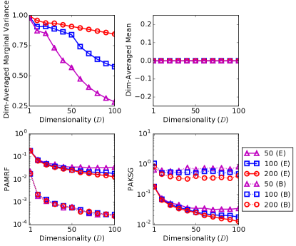
Figure 1: Results for inferring $p(\mathbf{x})=\mathcal{N}(\mathbf{x}|\bm{0},\mathbf{I})$ using SVGD with the RBF kernel, where particles are initialized by $\mathcal{N}(\mathbf{x}|\bm{0},25\mathbf{I})$. Top two figures show the dimension-averaged marginal variance $\frac{1}{D}\sum_{d=1}^{D}\mathrm{Var}_{\hat{q}_{M}}(x_{d})$ and mean $\frac{1}{D}\sum_{d=1}^{D}\mathbb{E}_{\hat{q}_{M}}[x_{d}]$ respectively, and bottom two figures show the particle-averaged magnitude of the repulsive force (PAMRF) $\frac{1}{M}\sum_{i=1}^{M}\|\mathbf{R}(\mathbf{x}^{(i)};\hat{q}_{M})\|_{\infty}$ and kernel smoothed gradient (PAKSG) $\frac{1}{M}\sum_{i=1}^{M}\|\mathbf{G}(\mathbf{x}^{(i)};p,\hat{q}_{M})\|_{\infty}$ respectively, at both the beginning (dotted;B) and the end of iterations (solid;E) with different number of particles $M=50,100$ and $200$.

First we highlight the importance of $\mathbf{R}(\mathbf{x};q)$. Referring to Eq. (2), we have $\phi^{*}(\mathbf{x})=\mathbf{G}(\mathbf{x};p,q)+\mathbf{R}(\mathbf{x};q)$, and we can show that the kernel smoothed gradient $\mathbf{G}(\mathbf{x};p,q)$ corresponds to the steepest direction for maximizing $\mathbb{E}_{\mathbf{x}\sim q}[\log p(\mathbf{x})]$, i.e.,

$$\frac{\mathbf{G}(\mathbf{x};p,q)}{\|\mathbf{G}(\mathbf{x};p,q)\|_{\mathcal{H}^{D}}}=\operatornamewithlimits{argmax}_{\|\bm{\phi}\|_{\mathcal{H}^{D}}\leq 1}\nabla_{\epsilon}\mathbb{E}_{\mathbf{z}\sim q_{[\bm{T}]}}[\log p(\mathbf{z})]|_{\epsilon=0},$$ (4)

where $\mathbf{z}=\bm{T}(\mathbf{x})=\mathbf{x}+\epsilon\bm{\phi}(\mathbf{x})$. The convergence condition $\mathbf{G}(\mathbf{x};p,q)\equiv\bm{0}$ corresponds to $\nabla_{\mathbf{y}}\log p(\mathbf{y})=\bm{0}$ for $q(\mathbf{y})\neq 0$, i.e., the optimal $q(\mathbf{x})$ collapses to modes of $p(\mathbf{x})$. This implies that without $\mathbf{R}(\mathbf{x};q)$, $\mathbf{G}(\mathbf{x};p,q)$ alone corresponds to the gradient method to find modes of $p(\mathbf{x})$. So $\mathbf{R}(\mathbf{x};q)$ is critical for SVGD to work as an inference algorithm for minimizing the KL divergence.

However, with a kernel measuring the global similarity in $\mathcal{X}\subset\mathbb{R}^{D}$ (e.g., the RBF kernel), the repulsive force becomes

$$\mathbf{R}(\mathbf{x};q)=\mathbb{E}_{\mathbf{y}\sim q}\left[\exp\left(-\frac{\|\mathbf{x}-\mathbf{y}\|_{2}^{2}}{2h}\right)\frac{\mathbf{x}-\mathbf{y}}{h}\right].$$

Unlike $\mathbf{G}(\mathbf{x};p,q)$ in which the bandwidth $h$ only appears as a denominator for $\|\mathbf{x}-\mathbf{y}\|_{2}^{2}$ and can be chosen using the median heuristic, the bandwidth in $\mathbf{R}(\mathbf{x};q)$ also appears as a denominator for $\mathbf{x}-\mathbf{y}$. As a result, finding a proper $h$ for $\mathbf{R}(\mathbf{x};q)$ will be hard and the magnitude of $\mathbf{R}(\mathbf{x};q)$ is bounded as

$$\|\mathbf{R}(\mathbf{x};q)\|_{\infty}\leq\mathbb{E}_{\mathbf{y}\sim q}\left[\frac{2}{e}\cdot\frac{\|\mathbf{x}-\mathbf{y}\|_{\infty}}{\|\mathbf{x}-\mathbf{y}\|_{2}^{2}}\right]$$ (5)

for any $h>0$. Intuitively, when $\|\mathbf{x}-\mathbf{y}\|_{\infty}/\|\mathbf{x}-\mathbf{y}\|_{2}^{2}\ll 1$ for most regions of $q$, $\|\mathbf{R}(\mathbf{x};q)\|_{\infty}$ would be small, making SVGD dynamics greatly dependent on $\mathbf{G}(\mathbf{x};p,q)$, especially in the beginning stage where $q$ does not match $p$ and $\|\mathbf{G}(\mathbf{x};p,q)\|_{\infty}$ is large. Besides, though the theoretical convergence condition that $\bm{\phi}^{*}(\mathbf{x})\equiv\bm{0}$ iff $q=p$ still holds, the vanishing repulsive force weakens it in reducing the difference between $\mathbf{G}(\mathbf{x};p,q)\equiv\bm{0}$ and $\bm{\phi}^{*}(\mathbf{x})\equiv\bm{0}$. These characteristics would bring problems in practice when $q$ is approximated by a set of particles $\{\mathbf{x}^{(i)}\}_{i=1}^{M}$: the empirical convergence condition $\hat{\phi}^{*}(\mathbf{x}^{(i)})=\bm{0},\forall i\in\{1,...,M\}$ does not guarantee $\{\mathbf{x}^{(i)}\}_{i=1}^{M}$ to be a good approximation of $p$, and the $\mathbf{G}(\mathbf{x};p,q)$-dominant dynamic would result in collapsing particles.

Now, a natural question is, for which $q$ does this intuition hold? One example is $q$ to be Gaussian as summarized in the following proposition:

Proposition 1.

Given the RBF kernel $k(\mathbf{x},\mathbf{y})$ and $q(\mathbf{y})=\mathcal{N}(\mathbf{y}|\bm{\mu},\bm{\Sigma})$, the repulsive force satisfies

$$\|\mathbf{R}(\mathbf{x};q)\|_{\infty}\leq\frac{\sqrt{D}}{\lambda_{\min}(\bm{\Sigma})(\frac{D}{2}+1)(1+\frac{2}{D})^{\frac{D}{2}}}\|\mathbf{x}-\bm{\mu}\|_{\infty},$$

where $\lambda_{\min}(\bm{\Sigma})$ is the smallest eigenvalue of $\bm{\Sigma}$. By using $\lim_{x\to 0}(1+x)^{1/x}=e$, we have $\|\mathbf{R}(\mathbf{x};q)\|_{\infty}\lesssim\|\mathbf{x}-\bm{\mu}\|_{\infty}/(\lambda_{\min}(\bm{\Sigma})\sqrt{D})$.

Proposition 1 indicates that the upper bound of $\|\mathbf{R}(\mathbf{x};q)\|_{\infty}$ negatively correlates with $D$. In practice, since $\mathbf{R}(\mathbf{x};\hat{q}_{M})$ is an unbiased estimate of $\mathbf{R}(\mathbf{x};q)$, we can also bound $\|\mathbf{R}(\mathbf{x};\hat{q}_{M})\|_{\infty}\lesssim\|\mathbf{x}-\bm{\mu}\|_{\infty}/(\lambda_{\min}(\bm{\Sigma})\sqrt{D})$. Apart from the Gaussian distribution, we can prove that such a negative correlation exists for $\mathbf{R}(\mathbf{x};\hat{q}_{M})$ in a more general case:

Proposition 2.

Let $k(\mathbf{x},\mathbf{y})$ be an RBF kernel. Suppose $q(\mathbf{y})$ is supported on a bounded set $\mathcal{X}$ which satisfies $\|\mathbf{y}\|_{\infty}\leq C$ for $\mathbf{y}\in\mathcal{X}$, and $\mathrm{Var}(y_{d}|y_{1},...,y_{d-1})\geq C_{0}$ almost surely for any $1\leq d\leq D$. Let $\{\mathbf{x}^{(i)}\}_{i=1}^{M}$ be a set of samples of $q$ and $\hat{q}_{M}$ the corresponding empirical distribution. Then, for any $\|\mathbf{x}\|_{\infty}\leq C$, $\alpha,\delta\in(0,1)$, there exists $D_{0}>0$, such that for any $D>D_{0}$,

$$\|R(\mathbf{x};\hat{q}_{M})\|_{\infty}\leq\frac{2}{eD^{\alpha}}$$ (6)

holds with at least probability $1-\delta$.

In proposition 2, the bounded support assumption is relatively mild: examples include distributions defined on the images, in which the pixel intensity lies in a bounded interval. Requiring the conditional variance is larger than some constant reflects that the stochasticity for each dimension will not be eliminated by knowing the values of other dimensions, which is a quite strong assumption. However, as evaluated in experiments, the negative correlation exists for $q$ even when such assumptions do not hold. Thus proposition 2 may be improved with weaker assumptions.

Given these intuitions, we would like to explain the particle degeneracy phenomenon in Fig. 1. As shown in the bottom row, there exists a negative correlation between $\|\mathbf{R}(\mathbf{x};\hat{q}_{M})\|_{\infty}$ and $D$, at both the beginning and the end of iterations. In the beginning stage, $\|\mathbf{G}(\mathbf{x};p,\hat{q}_{M})\|_{\infty}$ keeps almost unchanged while $\|\mathbf{R}(\mathbf{x};\hat{q}_{M})\|_{\infty}$ negatively correlates with $D$. This implies that the SVGD dynamics becomes more $\mathbf{G}(\mathbf{x};p,\hat{q}_{M})$-dominant with larger $D$ at the beginning. When converged, $\hat{\bm{\phi}}^{*}(\mathbf{x}^{(i)})=0$, which corresponds to $\|\mathbf{G}(\mathbf{x}^{(i)};p,\hat{q}_{M})\|_{\infty}=\|\mathbf{R}(\mathbf{x}^{(i)};\hat{q}_{M})\|_{\infty}$. In this case, we find an interesting phenomenon that $\|\mathbf{R}(\mathbf{x};\hat{q}_{M})\|_{\infty}$ tends to be constant with $M=50$ but the marginal variance still decreases with increasing dimensions. A possible explanation for this case is that assuming $q$ is Gaussian with $\bm{\Sigma}=\sigma^{2}\mathbf{I}$, the variance $\sigma^{2}=\lambda_{\min}(\bm{\Sigma})\lesssim\|\mathbf{x}^{(i)}-\bm{\mu}\|_{\infty}/(\|\mathbf{R}(\mathbf{x}^{(i)};\hat{q}_{M})\|_{\infty}\sqrt{D})$ as proved in proposition 1. When $\|\mathbf{R}(\mathbf{x}^{(i)};\hat{q}_{M})\|_{\infty}$ is almost constant (and $\|\mathbf{x}^{(i)}-\bm{\mu}\|_{\infty}$ does not increase faster than $\sqrt{D}$), $\sigma^{2}$ will decrease as $D$ increases.

4 Message Passing SVGD

As discussed in Section 3, the unsatisfying property of SVGD comes from the negative correlation between the dimensionality and the repulsive force. Though the high-dimensional nature of $p(\mathbf{x})$ is inevitable in practice, this problem can be solved for $p(\mathbf{x})$ with conditional independence structure, which is commonly described by probabilistic graphical models (PGMs). Based on this idea, we propose Message Passing SVGD, which converts the original high-dimensional inference problem into a set of local inference problems with lower dimensions.

More specifically, we assume $p(\mathbf{x})$ can be factorized as $p(\mathbf{x})\propto\prod_{F\in\mathcal{F}}\psi_{F}(\mathbf{x}_{F})$ where the factor $F\subset\{1,...,D\}$ denotes the index set and $\mathbf{x}_{F}=[x_{d}]_{d\in F}$. The Markov blanket $\Gamma_{d}=\cup\{F:F\ni d\}\setminus\{d\}$ contains neighborhood nodes of $d$ such that $p(x_{d}|\mathbf{x}_{\neg d})=p(x_{d}|\mathbf{x}_{\Gamma_{d}})$.

4.1 A Decomposition of the KL Divergence

Our method relies on the key observation that we can decompose $\mathrm{KL}(q\|p)$ as

$$\mathrm{KL}(q\|p) =\mathrm{KL}\big{(}q(x_{d}|\mathbf{x}_{\neg d})q(\mathbf{x}_{\neg d})\big{\|}p(x_{d}|\mathbf{x}_{\Gamma_{d}})q(\mathbf{x}_{\neg d})\big{)}$$ (7)

$$\leavevmode\nobreak\ \leavevmode\nobreak\ \leavevmode\nobreak\ \leavevmode\nobreak\ +\mathrm{KL}\big{(}q(\mathbf{x}_{\neg d})\big{\|}p(\mathbf{x}_{\neg d})\big{)},$$

where $\neg d=\{1,...,D\}\setminus\{d\}$ denotes the index set other than $d$. Eq. (7) provides another perspective for minimizing $\mathrm{KL}(q\|p)$: instead of solving a global problem which minimizes $\mathrm{KL}(q\|p)$ over $q(\mathbf{x})$, we can iteratively solve a set of local problems which minimizes the localized divergence over $q(x_{d}|\mathbf{x}_{\neg d})$ by keeping $q(\mathbf{x}_{\neg d})$ fixed, i.e.,

$$\operatornamewithlimits{argmin}_{q(x_{d}|\mathbf{x}_{\neg d})}\mathrm{KL}\big{(}q(x_{d}|\mathbf{x}_{\neg d})q(\mathbf{x}_{\neg d})\big{\|}p(x_{d}|\mathbf{x}_{\Gamma_{d}})q(\mathbf{x}_{\neg d})\big{)}.$$ (8)

This idea resembles EP, which also performs local minimizations iteratively, however, for a localized version of the inclusive KL divergence $\mathrm{KL}(p\|q)$ (Minka, 2001). Another difference is that each local step in EP does not guarantees minimizing a global divergence (Minka, 2005), while solving Problem (8) iteratively corresponds to minimizing the original $\mathrm{KL}(q\|p)$ due to the decomposition in Eq. (7).

Eq. (7) requires decomposing $q(\mathbf{x})$ as $q(x_{d}|\mathbf{x}_{\neg d})$ for each $d$, which makes it useless for VI methods with a parametric $q(\mathbf{x})$ except some special cases (e.g., $q(\mathbf{x})$ is Gaussian or fully factorized as $q(\mathbf{x})=\prod_{d=1}^{D}q(x_{d})$). However, this decomposition is very suitable for transformation based methods like SVGD. Consider the transformation $\mathbf{z}=\bm{T}(\mathbf{x})=[x_{1},...,T_{d}(x_{d}),...,x_{D}]^{\top}$ for $\mathbf{x}\sim q$, where only the $d$th dimension is transformed and other dimensions are kept unchanged, we have $q_{[\bm{T}]}(\mathbf{z}_{\neg d})=q(\mathbf{z}_{\neg d})$. In other words, minimizing $\mathrm{KL}(q_{[\bm{T}]}\|p)$ over $T_{d}$ is equivalent to minimizing $\mathrm{KL}\big{(}q_{[T_{d}]}(x_{d}|\mathbf{x}_{\neg d})q(\mathbf{x}_{\neg d})\big{\|}p(x_{d}|\mathbf{x}_{\Gamma_{d}})q(\mathbf{x}_{\neg d})\big{)}$.

Thus SVGD can be applied to Problem (8) directly, by following $T_{d}:x_{d}\to x_{d}+\epsilon\phi_{d}(\mathbf{x})$ where $\phi_{d}\in\mathcal{H}_{0}$ is associated with the global kernel $k:\mathcal{X}\times\mathcal{X}\to\mathbb{R}$, and solving $\min_{\|\phi_{d}\|_{\mathcal{H}_{0}}\leq 1}\nabla_{\epsilon}\mathrm{KL}(q_{[\bm{T}]}\|p)\big{|}_{\epsilon=0}$. This produces a coordinate-wise version of SVGD. However, the high-dimensional problem still exists due to the global kernel. To reduce the dimensionality, we further restrict the transformation to be dependent only on $x_{d}$ and its Markov blanket, i.e., $T_{d}:x_{d}\to x_{d}+\epsilon\phi_{d}(\mathbf{x}_{S_{d}})$, $\phi_{d}\in\mathcal{H}_{d}$, where $S_{d}=\{d\}\cup\Gamma_{d}$. Here $\mathcal{H}_{d}$ is the RKHS induced by kernel $k_{d}:\mathcal{X}_{S_{d}}\times\mathcal{X}_{S_{d}}\to\mathbb{R}$, where $\mathcal{X}_{S_{d}}=\{\mathbf{x}_{S_{d}},\mathbf{x}\in\mathcal{X}\}$. By doing so, we have the following proposition:

Proposition 3.

Let $\mathbf{z}=\bm{T}(\mathbf{x})=[x_{1},...,T_{d}(x_{d}),...,x_{D}]^{\top}$ with $T_{d}:x_{d}\to x_{d}+\epsilon\phi_{d}(\mathbf{x}_{S_{d}})$, $\phi_{d}\in\mathcal{H}_{d}$ where $\mathcal{H}_{d}$ is associated with the local kernel $k_{d}:\mathcal{X}_{S_{d}}\times\mathcal{X}_{S_{d}}\to\mathbb{R}$. Then, we have

$$\nabla_{\epsilon}\mathrm{KL}(q_{[\bm{T}]}||p)=$$ (9)

$$\leavevmode\nobreak\ \leavevmode\nobreak\ \leavevmode\nobreak\ \leavevmode\nobreak\ \leavevmode\nobreak\ \leavevmode\nobreak\ \nabla_{\epsilon}\mathrm{KL}\big{(}q_{[T_{d}]}(z_{d}|\mathbf{z}_{\Gamma_{d}})q(\mathbf{z}_{\Gamma_{d}})\big{\|}p(z_{d}|\mathbf{z}_{\Gamma_{d}})q(\mathbf{z}_{\Gamma_{d}})\big{)},$$

and the solution for $\min_{\|\phi_{d}\|_{\mathcal{H}_{d}}\leq 1}\nabla_{\epsilon}\mathrm{KL}(q_{[\bm{T}]}|\|p)|_{\epsilon=0}$ is $\phi_{d}^{*}/\|\phi_{d}^{*}\|_{\mathcal{H}_{d}}$, where

$$\phi_{d}^{*}(\mathbf{x}_{S_{d}})= \mathbb{E}_{\mathbf{y}_{S_{d}}\sim q}\big{[}k_{d}(\mathbf{x}_{S_{d}},\mathbf{y}_{S_{d}})\nabla_{y_{d}}\log p(y_{d}|\mathbf{y}_{\Gamma_{d}})$$ (10)

$$+\nabla_{y_{d}}k_{d}(\mathbf{x}_{S_{d}},\mathbf{y}_{S_{d}})\big{]}.$$

As shown in Eq. (10), computing $\phi^{*}(\mathbf{x}_{S_{d}})$ only requires $\mathbf{x}_{S_{d}}\in\mathcal{X}_{S_{d}}$ instead of $\mathbf{x}\in\mathcal{X}$, which reduces the dimension from $D$ to $|S_{d}|$. This would alleviate the vanishing repulsive force problem , especially for the case where $p(\mathbf{x})$ is highly sparse structured such that $|S_{d}|\ll D$ (e.g., pairwise Markov Random Fields), as verified in the experiments on both synthetic and real-world problems.

Similar to the original SVGD, the convergence condition $\phi_{d}^{*}(\mathbf{x}_{S_{d}})\equiv 0$ holds iff $q(x_{d}|\mathbf{x}_{\Gamma_{d}})q(\mathbf{x}_{\Gamma_{d}})\equiv p(x_{d}|\mathbf{x}_{\Gamma_{d}})q(\mathbf{x}_{\Gamma_{d}})$, i.e., $q(x_{d}|\mathbf{x}_{\Gamma_{d}})\equiv p(x_{d}|\mathbf{x}_{\Gamma_{d}})$ when $k_{d}(\mathbf{x}_{S_{d}},\mathbf{y}_{S_{d}})$ is strictly positive definite in a proper sense (Liu et al., 2016; Chwialkowski et al., 2016). In other words, to reduce the dimension, we have to pay the price that $q$ is only conditionally consistent with $p$. This relaxation of $q$ also appears in traditional methods like loopy BP and its variants, in which only marginal consistency is guaranteed (Wainwright & Jordan, 2008).

4.2 Markov Blanket based Kernels

Now, the remaining question is the choice of the local kernel $k_{d}:\mathcal{X}_{S_{d}}\times\mathcal{X}_{S_{d}}\to\mathbb{R}$. We can simply define $k_{d}(\mathbf{x}_{S_{d}},\mathbf{y}_{S_{d}})=f\big{(}\|\mathbf{x}_{S_{d}}-\mathbf{y}_{S_{d}}\|_{2}^{2}/(2h_{S_{d}})\big{)}$ for $f(z)=\exp(-z)$ (i.e., the RBF kernel), with the implicit assumption that all nodes in the Markov blanket contribute equally for node $d$. We call such a $k_{d}$ the Single-Kernel. However, as the factorization of $p(\mathbf{x})\propto\prod_{F\in\mathcal{F}}\psi_{F}(\mathbf{x}_{F})$ is known, we can also define the Multi-Kernel where $k_{d}(\mathbf{x}_{S_{d}},\mathbf{y}_{S_{d}})=\frac{1}{K}\sum_{F\ni d}f\big{(}\|\mathbf{x}_{F}-\mathbf{y}_{F}\|_{2}^{2}/(2h_{F})\big{)}$, where $K$ is the number of factors containing $d$, to reflect the assumption that nodes in different factors may contribute in a different way. By doing so, $R_{d}(\mathbf{x};q)=\frac{1}{K}\sum_{F\ni d}\mathbb{E}_{\mathbf{y}_{F}\in q}\big{[}\nabla_{y_{d}}f\big{(}\|\mathbf{x}_{F}-\mathbf{y}_{F}\|_{2}^{2}/(2h_{F})\big{)}\big{]}$ and we can further reduce the dimension for $R_{d}(\mathbf{x};q)$ from $|S_{d}|$ to $\max\{|F|:F\ni d\}$.

4.3 Final Algorithm

Similar to SVGD, we use a set of particles $\{\mathbf{x}^{(i)}\}_{i=1}^{M}$ to approximate $q$ and this procedure is summarized in Algorithm 1. According to the choice of kernels, we abbreviate MP-SVGD-s for the Single-Kernel and MP-SVGD-m for the Multi-Kernel.

0:  A differentiable target distribution $p(\mathbf{x})$ whose $d$th conditional distribution is $p(x_{d}|\mathbf{x}_{\Gamma_{d}})=p(x_{d}|\mathbf{x}_{-d})$, and a set of initial particles $\{\mathbf{x}^{(i)}\}_{i=1}^{M}$.

0:  A set of particles $\{\mathbf{x}^{(i)}\}_{i=1}^{M}$ as an approximation of $p(\mathbf{x})$.

  for iteration $t$ do

     for $d\in\{1,...,D\}$ do

        $\mathbf{x}^{(i)}_{d}\leftarrow\mathbf{x}_{d}^{(i)}+\epsilon\hat{\phi}_{d}^{*}(\mathbf{x}_{S_{d}}^{(i)})$ where $\epsilon$ is the stepsize, and

$$\hat{\phi}^{*}_{d}(\mathbf{x}_{S_{d}}) =\mathbb{E}_{\mathbf{y}_{S_{d}}\sim\hat{q}_{M}}[k_{d}(\mathbf{x}_{S_{d}},\mathbf{y}_{S_{d}})\nabla_{y_{d}}\log p(y_{d}|\mathbf{y}_{\Gamma_{d}})$$

$$\leavevmode\nobreak\ \leavevmode\nobreak\ \leavevmode\nobreak\ \leavevmode\nobreak\ +\nabla_{y_{d}}k_{d}(\mathbf{x}_{S_{d}},\mathbf{y}_{S_{d}})].$$

     end for

  end for

Algorithm 1 Message Passing SVGD

Updating particles acts in a message passing way as shown in Figure 2: node $d$ receives particles (messages) from its neighbors (i.e., $\{\mathbf{x}_{\Gamma_{d}}^{(i)}\}_{i=1}^{M}$); updates its own particles $\{\mathbf{x}_{d}^{(i)}\}_{i=1}^{M}$; and sends them to its neighbors. Unlike loopy BP, each node sends the same message to its neighbors. This resembles VMP, where messages from the parent to its children in a directed graph are also identical (Winn & Bishop, 2005).

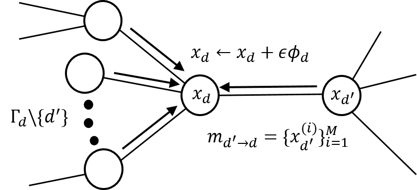
Figure 2: Message passing procedure for node $d$.

5 Experiments

In this section, we experimentally verify our analysis and evaluate the performance of MP-SVGD with other inference methods on both synthetic and real-world examples. We use the RBF kernel with the bandwidth chosen by the median heuristic for all experiments.

5.1 Synthetic Markov Random Fields

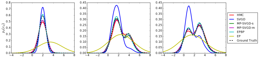
Figure 3: A qualitative comparison of inference methods with 100 particles (except EP) for marginal densities of three randomly selected nodes. Density curves of SVGD, MP-SVGD and HMC are estimated by kernel density estimator with RBF kernels. For EPBP, the curve is drawn by normalizing its beliefs over the fixed interval $[-5,10)$ with bin size $0.01$.

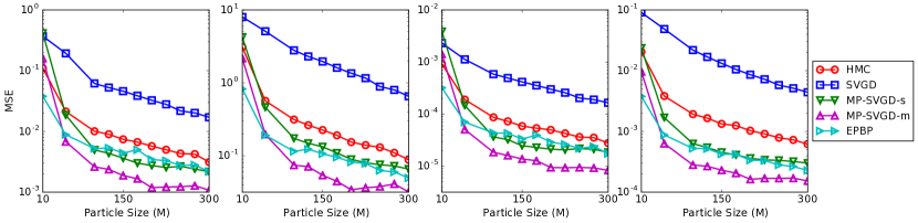
Figure 4: A quantitative comparison of inference methods with varying number of particles. Performance is measured by the MSE of the estimation of expectation $\mathbb{E}_{\mathbf{x}\sim\hat{q}_{M}}[\mathbf{f}(\mathbf{x})]$ for test functions $\mathbf{f}(\mathbf{x})=\mathbf{x}$, $\mathbf{x}^{2}$, $1/(1+\exp(\bm{\omega}\circ\mathbf{x}+\mathbf{b}))$ and $\cos(\bm{\omega}\circ\mathbf{x}+\mathbf{b})$, arranged from left to right, where $\circ$ denotes the element-wise product. Results are averaged over 10 random draws of $\bm{\omega}$ and $\mathbf{b}$, where $\bm{\omega},\mathbf{b}\in\mathbb{R}^{100}$ with $\omega_{d}\sim\mathcal{N}(0,1)$ and $b_{d}\in\mathrm{Uniform}[0,2\pi]$, $\forall d\in\{1,...,100\}$.

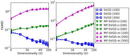
Figure 5: PAMRF $\frac{1}{M}\sum_{i=1}^{M}\|\mathbf{R}(\mathbf{x}^{(i)};\hat{q}_{M})\|_{r}$ for converged $\{\mathbf{x}^{(i)}\}_{i=1}^{M}$ with $r=\infty$ (left) and $r=2$ (right). The grid size ranges from $2\times 2$ to $10\times 10$. The number in the bracket denotes the number of particles.

We follow the settings of (Lienart et al., 2015) and focus on a pairwise MRF on the 2D grid $p(\mathbf{x})\propto\prod_{d\in\mathcal{V}}\psi_{d}(x_{d})\prod_{(d,t)\in\mathcal{E}}\psi_{dt}(x_{d},x_{t})$ with the random variable in each node taking values on $\mathbb{R}$. The node and edge potentials are chosen such that $p(\mathbf{x})$ and its marginals are multimodal, non-Gaussian and skewed:

$$\left\{\begin{array}[]{l}\psi_{d}(x_{d})=\alpha_{1}\mathcal{N}(x_{d}-y_{d}|-2,1)+\alpha_{2}\mathcal{G}(x_{d}-y_{d}|2,1.3)\\ \psi_{dt}(x_{d},x_{t})=\mathcal{L}(x_{d}-x_{t}|0,2)\end{array},\right.$$ (11)

where $y_{d}$ denotes the observed value at node $d$ and is initialized randomly as $y_{d}\sim\alpha_{1}\mathcal{N}(y_{d}-2|-2,1)+\alpha_{2}\mathcal{G}(y_{d}-2|2,1.3)$, $\mathcal{N}(x|\mu,\sigma^{2})\propto\exp(-(x-\mu)^{2}/(2\sigma^{2}))$, $\mathcal{G}(x|\mu,\beta)\propto\exp(-(x-\mu)/\beta+\exp(-(x-\mu)/\beta))$ and $\mathcal{L}(x|\mu,\beta)\propto\exp(-|x-\mu|/\beta)$ denote the density of Gaussian, Gumbel and Laplace distribution, respectively. Parameters $\alpha_{1}$ and $\alpha_{2}$ are set to 0.6 and 0.4. We consider a $10\times 10$ grid except Fig. 5, whose grid size ranges from $2\times 2$ to $10\times 10$. All experimental results are averaged over 10 runs with random initializations.

Since $p(\mathbf{x})$ is intractable, we recover the ground truth by samples drawn by an adaptive version of Hamiltonian Monte Carlo (HMC) (Neal, 2011; Shi et al., 2017). We run 100 chains in parallel with 40,000 samples for each chain after 10,000 burned-in, i.e. 4 million samples in total.

We compare MP-SVGD with SVGD, HMC, EP and EPBP (Lienart et al., 2015). Although widely used in MRFs, Gibbs sampling does not suit this task since the conditional distribution $p(x_{d}|\mathbf{x}_{\Gamma_{d}})$ cannot be sampled directly. So we use uniformly randomly chosen particles from the 4 million ground truth samples as a strong baseline and regard the method as HMC. For EP, we use the Gaussian distribution as the factors, and the moment matching step is done by numerical integration due to the non-Gaussian nature of $p(\mathbf{x})$. EPBP is a variant of BP methods and the original state-of-the-art method on this task. It uses weighted samples to estimate the messages while other methods (except EP) use unweighted samples to approximate $p(\mathbf{x})$ directly.

Fig. 3 provides a qualitative comparison of these methods by visualizing the estimated marginal densities on each node. As is shown, SVGD estimates the marginals undesirably in all cases. For both unimodal and bimodal cases, the SVGD curve exhibits a sharp, peaked behavior, indicating the collapsing trend of its particles. It is interesting to note that in the rightmost figure, more SVGD particles gather around the lower mode. One possible reason is that the lower marginal mode may correspond to a larger mode in the joint distribution, into which SVGD particles tends to collapse. EP provides quite a crude approximation as expected, due to the mismatch between its Gaussian assumption and the non-Gaussian nature of $p(\mathbf{x})$. Other methods perform similarly.

Fig. 4 provides a quantitative comparison in particle efficiency measured by the mean squared error (MSE) of estimated expectation with different particle sizes $M$. For EPBP, $M$ denotes the number of node particles when approximating messages. We observe that SVGD achieves the highest RMSE compared to other methods, reflecting its particle degeneracy. Compared to HMC and EPBP, MP-SVGD achieves comparable and even better results. Besides, MP-SVGD-m achieves lower RMSE than MP-SVGD-s, reflecting the benefits of MP-SVGD-m of leveraging more structural information in designing local kernels.

Fig. 5 compares MP-SVGD with SVGD in particle-averaged magnitude of the repulsive force (PAMRF) $\frac{1}{M}\sum_{i=1}^{M}\|\mathbf{R}(\mathbf{x}^{(i)};\hat{q}_{M})\|_{r}$ at the end of iterations for various dimensions. As expected, the SVGD PAMRF negatively correlates with the dimensionality $D$ while the MP-SVGD PAMRF does not. Besides, both of them exhibit roughly a log linear relationship with the dimensionality. This verifies Proposition 2 that $\|\mathbf{R}(\mathbf{x}^{(i)};\hat{q}_{M})\|_{\infty}$ is upper bounded by $D^{-\alpha}$ for some constant $\alpha$. This also reflects the power of MP-SVGD in preventing the repulsive force from being too small by reducing dimensionality using local kernels. Besides, we observe that MP-SVGD-m PAMRF is higher than MP-SVGD-s PAMRF, which verifies our analysis regarding Single-Kernel and Multi-Kernel: for the pairwise MRF, the dimension for Single-Kernel is $5$ at most (the Markov blanket and the node itself) while the dimension for Multi-Kernel is $2$ at most (the edge) and thus lower dimensionality corresponds to higher repulsive force.

5.2 Image Denoising

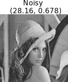
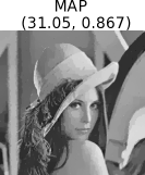
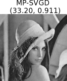
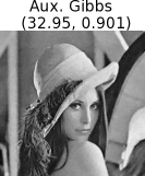
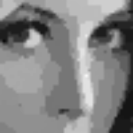
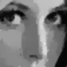
Figure 6: Denoising results for Lena using 50 particles, $256\times 256$ pixels, $\sigma_{n}=10$. The number in bracket is PSNR and SSIM. Upper Row: The full size image; Bottom Row: The $50\times 50$ patches.

Our last experiment is designed for verifying the power of MP-SVGD in real-world application. Following (Schmidt et al., 2010), we formulate image denoising via finding the posterior mean of $p(\mathbf{x}|\mathbf{y})\propto p(\mathbf{y}|\mathbf{x})p(\mathbf{x})$, where the likelihood $p(\mathbf{y}|\mathbf{x})=\mathcal{N}(\mathbf{y}|\mathbf{x},\sigma_{n}^{2}\mathbf{I})$ denotes that the observed image $\mathbf{y}=\mathbf{x}+\mathbf{n}$ for some unknown natural image $\mathbf{x}$ corrupted by Gaussian noise $\mathbf{n}$ with the noise level $\sigma_{n}$. The prior $p(\mathbf{x})$ encodes the statistics of natural images, which is a Fields-of-Experts (FOE) (Roth & Black, 2009) MRF:

$$p(\mathbf{x})\propto\exp(-\frac{\epsilon\|\mathbf{x}\|_{2}^{2}}{2})\prod_{F\in\mathcal{F}}\prod_{i=1}^{N}\phi(\mathbf{J}_{i}^{\mathrm{T}}\mathbf{x}_{F};\bm{\alpha}_{i}),$$ (12)

where $\{\mathbf{J}_{i}\}_{i=1}^{N}$ is a bank of linear filters and the expert function $\phi(\mathbf{J}_{i}^{\mathrm{T}}\mathbf{x}_{F};\bm{\alpha}_{i})=\sum_{j=1}^{J}\alpha_{ij}\mathcal{N}(\mathbf{J}_{i}^{\mathrm{T}}\mathbf{x}_{F}|0,\sigma_{i}^{2}/s_{j})$ is the Gaussian scale mixtures (Woodford et al., 2009). We focus on the pairwise MRF where $\mathcal{F}$ indexes all the edge factors, $\mathbf{J}_{i}=[1,-1]^{\top}$, $N=1$ and $J=15$. All the parameters (i.e., $\epsilon$, $J_{i}$, $\sigma_{i}$ and $s_{j}$) are pre-learned and details can be found in (Schmidt et al., 2010).

We compare SVGD and MP-SVGD with Gibbs sampling with auxiliary variables (Aux. Gibbs), the state-of-the-art method reported in the original paper. The recovered image is obtained by averaging all the particles and its quality is evaluated using the peak signal-to-noise ratio (PSNR) and structural similarity index (SSIM) (Wang et al., 2004). Higher PSNR/SSIM generally means better image quality.

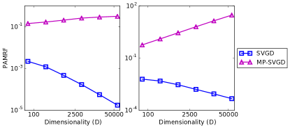
Figure 7: PAMRF $\frac{1}{M}\sum_{i=1}^{M}\|\mathbf{R}(\mathbf{x}^{(i)};\hat{q}_{M})\|_{r}$ for converged $\{\mathbf{x}^{(i)}\}_{i=1}^{M}$ with $r=\infty$ (left) and $r=2$ (right) over rescaled Lena ranged from $8\times 8$ to $256\times 256$. $M=50$ particles are used.

Fig. 6 shows example results for Lena, a benchmark image for comparing denoising methods. Despite the difference in PSNR and SSIM, the image recovered by SVGD lack texture details (especially for the region near the nose of Lena shown in the $50\times 50$ patches), which resembles the image reconstructed by MAP.

Table 1 compares these method quantitatively. As expected, MP-SVGD achieves the best result given the same number of particles. We also find that Aux. Gibbs requires about $200$ particles for $\sigma_{n}=10$ and $400$ to $800$ particles for $\sigma_{n}=20$, to achieve a similar performance of MP-SVGD.

From Fig. 7 we observe a negative/non-negative correlation between the repulsive force and the dimensionality for SVGD/MP-SVGD, respectively, which verifies our analysis again.

Table 1: Denoising results for 10 test images (Lan et al., 2006) from BSD dataset (Martin et al., 2001). The first two rows are cited from (Schmidt et al., 2010) while the other rows are based on our implementation. $M$ denotes the number of particles.

Inference	avg. PSNR		avg. SSIM
	$\sigma_{n}=10$	$\sigma_{n}=20$	$\sigma_{n}=10$	$\sigma_{n}=20$
MAP	30.27	26.48	0.855	0.720
Aux. Gibbs	32.09	28.32	0.904	0.808
Aux. Gibbs ($M=50$)	31.87	28.05	0.898	0.795
Aux. Gibbs ($M=100$)	31.98	28.17	0.901	0.801
SVGD ($M=50$)	31.58	27.86	0.894	0.766
SVGD ($M=100$)	31.65	27.90	0.896	0.767
MP-SVGD ($M=50$)	32.09	28.21	0.905	0.808
MP-SVGD ($M=100$)	32.12	28.27	0.906	0.809

6 Conclusions and Future Work

In this paper, we analyze the particle degeneracy phenomenon of SVGD in high dimensions and attribute it to the negative correlation between the repulsive force and dimensionality. We also propose message passing SVGD (MP-SVGD), which converts the original problem into several local inference problem with lower dimensions, to solve this problem. Experiments on both synthetic and real-world applications show the effectiveness of MP-SVGD.

For future work, we’d like to settle the analysis of the repulsive force and its impact on SVGD dynamics completely and formally. We also want to apply MP-SVGD to more complex real-world applications like pose estimation (Pacheco et al., 2014). Besides, investigating robust kernel with non-decreasing repulsive force is also an interesting direction.

References

- Aggarwal et al. (2001) Aggarwal, C. C., Hinneburg, A., and Keim, D. A. On the surprising behavior of distance metrics in high dimensional spaces. In Proceedings of the International conference on database theory, 2001.
- Chwialkowski et al. (2016) Chwialkowski, K., Strathmann, H., and Gretton, A. A kernel test of goodness of fit. In Proceedings of the International Conference on Machine Learning, 2016.
- Feng et al. (2017) Feng, Y., Wang, D., and Liu, Q. Learning to draw samples with amortized stein variational gradient descent. In Proceedings of the Conference on Uncertainty in Artificial Intelligence, 2017.
- Gorham & Mackey (2017) Gorham, J. and Mackey, L. Measuring sample quality with kernels. In Proceedings of the International Conference on Machine Learning, 2017.
- Haarnoja et al. (2017) Haarnoja, T., Tang, H., Abbeel, P., and Sergey, L. Reinforcement learning with deep energy-based policies. In Proceedings of the International Conference on Machine Learning, 2017.
- Ihler & Mcallester (2009) Ihler, A. T. and Mcallester, D. A. Particle belief propagation. In Proceedings of the International Conference on Artificial Intelligence and Statistics, 2009.
- Koller & Friedman (2009) Koller, D. and Friedman, N. Probabilistic graphical models: principles and techniques. MIT press, 2009.
- Lan et al. (2006) Lan, X., Roth, S., Huttenlocher, D., and Black, M. J. Efficient belief propagation with learned higher-order markov random fields. In European conference on computer vision, 2006.
- Lienart et al. (2015) Lienart, T., Teh, Y. W., and Doucet, A. Expectation particle belief propagation. In Advances in Neural Information Processing Systems, 2015.
- Liu & Wang (2016) Liu, Q. and Wang, D. Stein variational gradient descent: A general purpose bayesian inference algorithm. In Advances In Neural Information Processing Systems, 2016.
- Liu et al. (2016) Liu, Q., Lee, J., and Jordan, M. A kernelized stein discrepancy for goodness-of-fit tests. In Proceedings of the International Conference on Machine Learning, 2016.
- Liu et al. (2017) Liu, Y., Ramachandran, P., Liu, Q., and Peng, J. Stein variational policy gradient. In Proceedings of the Conference on Uncertainty in Artificial Intelligence, 2017.
- Martens & Sutskever (2010) Martens, J. and Sutskever, I. Parallelizable sampling of markov random fields. In Proceedings of the International Conference on Artificial Intelligence and Statistics, 2010.
- Martin et al. (2001) Martin, D., Fowlkes, C., Tal, D., and Malik, J. A database of human segmented natural images and its application to evaluating segmentation algorithms and measuring ecological statistics. In IEEE International Conference on Computer Vision, 2001.
- Minka (2001) Minka, T. Expectation propagation for approximate bayesian inference. In Proceedings of the Conference on Uncertainty in Artificial Intelligence, 2001.
- Minka (2005) Minka, T. Divergence measures and message passing. Technical Report MSR-TR-2005-173, Microsoft Research, 2005.
- Neal (2011) Neal, R. M. Mcmc using hamiltonian dynamics. Handbook of Markov Chain Monte Carlo, 2(11), 2011.
- Pacheco et al. (2014) Pacheco, J., Zuffi, S., Black, M., and Sudderth, E. Preserving modes and messages via diverse particle selection. In Proceedings of the International Conference on Machine Learning, 2014.
- Pearl (1988) Pearl, J. Probabilistic reasoning in intelligent systems: networks of plausible inference. Morgan Kaufmann, 1988.
- Pu et al. (2017) Pu, Y., Gan, Z., Henao, R., Li, C., Han, S., and Carin, L. Vae learning via stein variational gradient descent. In Advances in Neural Information Processing Systems, 2017.
- Ramdas et al. (2015) Ramdas, A., Reddi, S. J., Póczos, B., Singh, A., and Wasserman, L. On the decreasing power of kernel and distance based nonparametric hypothesis tests in high dimensions. In Proceedings of the AAAI Conference on Artificial Intelligence, 2015.
- Roth & Black (2009) Roth, S. and Black, M. J. Fields of experts. International Journal of Computer Vision, 2009.
- Schmidt et al. (2010) Schmidt, U., Gao, Q., and Roth, S. A generative perspective on mrfs in low-level vision. In Computer Vision and Pattern Recognition, 2010.
- Scholkopf & Smola (2001) Scholkopf, B. and Smola, A. J. Learning with kernels: support vector machines, regularization, optimization, and beyond. MIT press, 2001.
- Shi et al. (2017) Shi, J., Chen, J., Zhu, J., Sun, S., Luo, Y., Gu, Y., and Zhou, Y. Zhusuan: A library for bayesian deep learning. arXiv preprint arXiv:1709.05870, 2017.
- Sudderth et al. (2003) Sudderth, E., Ihler, A., Freeman, W., and Willsky, A. Nonparametric belief propagation. In Computer Vision and Pattern Recognition, 2003.
- Wainwright & Jordan (2008) Wainwright, M. J. and Jordan, M. I. Graphical models, exponential families, and variational inference. Foundations and Trends® in Machine Learning, 2008.
- Wang et al. (2017) Wang, D., Zeng, Z., and Liu, Q. Structured stein variational inference for continuous graphical models. arXiv preprint arXiv:1711.07168, 2017.
- Wang et al. (2004) Wang, Z., Bovik, A. C., Sheikh, H. R., and Simoncelli, E. P. Image quality assessment: from error visibility to structural similarity. IEEE transactions on image processing, 2004.
- Winn & Bishop (2005) Winn, J. and Bishop, C. M. Variational message passing. Journal of Machine Learning Research, 2005.
- Woodford et al. (2009) Woodford, O. J., Rother, C., and Kolmogorov, V. A global perspective on map inference for low-level vision. In IEEE International Conference on Computer Vision, 2009.