Theory of Kerr Instability Amplification

Abstract

A new amplification method based on the optical Kerr instability is suggested and theoretically analyzed, with emphasis on the near- to mid-infrared wavelength regime. Our analysis for CaF₂ and KBr crystals shows that one to two cycle pulse amplification by 3-4 orders of magnitude in the wavelength range from $1-14\,\mu$m is feasible with currently available laser sources. At $14\,\mu$m final output energies in the 50 $\mu$J range are achievable corresponding to about 0.2-0.25% of the pump energy. The Kerr instability presents a promising process for the amplification of ultrashort mid-infrared pulses.

1 Introduction

Research in strong field physics and attosecond science has triggered the need for high intensity ultrashort laser sources in the mid-infrared [1, 2, 3]. Currently, the most common generation and amplification methods are based on the second order nonlinearity, such as optical parametric amplifiers (OPAs) [4, 5, 6]; recently the potential for single cycle infrared pulse generation by difference frequency generation has been demonstrated [7].

Although OPAs are currently the leading technology for ultrashort mid-infrared pulse amplification, their development is challenging. For their efficient operation a series of stringent conditions must be met which are intimately connected to the properties of second order nonlinear crystals. Amplification of single-cycle pulses either requires thin crystals (reducing the efficiency), or low dispersion across a spectrum covering the frequencies of the three interacting waves. Moreover, many second-order nonlinear crystals absorb light in the mid-infrared, and moderate damage thresholds also present a limitation.

Here we introduce an alternative concept for mid-infrared amplification based on the Kerr nonlinearity which we call Kerr instability amplification (KIA). In a Kerr nonlinear material parametric four wave mixing processes of the type $\omega_{p}+\omega_{p}-(\omega_{p}\pm\Omega_{s})=\omega_{p}\mp\Omega_{s}$ occur, during which two photons $\omega_{p}$ of the pump field are converted into fields $\varepsilon_{x}(\Omega_{s})$ and $\varepsilon_{x}^{*}(-\Omega_{s})$ with photon energies shifted to the red and blue side of $\omega_{p}$ by $\Omega_{s}$, see Fig. 1. We find that for a wide range of seed frequencies in the interval $-\omega_{p}<\Omega_{s}<\omega_{p}$ there exist transverse wavevectors $k_{\!\perp}$ for which unstable behavior occurs that results in exponential growth. As the transverse wavevector for maximum amplification $\bar{k}_{\!\perp}(\Omega_{s})$ is finite, emission is noncollinear with the pump pulse. Mathematically, the instability emerges from a coupling between the wave equations for $\varepsilon_{x}(\Omega_{s})$ and $\varepsilon^{*}_{x}(-\Omega_{s})$. This yields a second order Mathieu-type equation that contains unstable solutions. The wavevectors of the instability $\mathbf{K}(\pm\Omega_{s})$ fulfill the relation $\mathbf{K}(\Omega_{s})=2\mathbf{k}_{p}+\mathbf{K}(-\Omega_{s})$, see Fig. 1, so that phase matching is automatically fulfilled. Outside the unstable range, the phases of $\varepsilon_{x}(\Omega_{s})$ and $\varepsilon_{x}^{*}(-\Omega_{s})$ are mismatched and regular four wave mixing dynamics ensues. Through this instability a Kerr nonlinear material irradiated by a high intensity pump pulse can act as an amplifier for a noncollinear seed pulse.

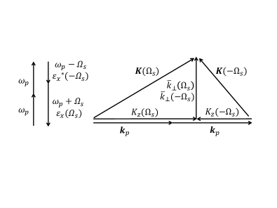
Figure 1: Schematic of Kerr instability amplification (KIA). Left: parametric four wave mixing process of the type $2\omega_{p}-(\omega_{p}\pm\Omega_{s})=\omega_{p}\mp\Omega_{s}$ where $\omega_{p}$ is the pump frequency and $-\omega_{p}<\Omega_{s}<\omega_{p}$ is the seed frequency. Right: there exist transverse wavevectors for which unstable behavior occurs; gain is maximum for the transverse wavevector $\bar{k}_{\perp}(\Omega_{s})$. The instability evolves as $\varepsilon_{x}(\Omega_{s})=\exp(i(\omega_{p}+\Omega_{s})t-i\mathbf{K}(\Omega_{s})\mathbf{x})$ and $\varepsilon_{x}^{*}(-\Omega_{s})=\exp(-i(\omega_{p}-\Omega_{s})t+i\mathbf{K}(-\Omega_{s})\mathbf{x})$. Here, $\mathbf{K}(\Omega_{s})=(\bar{k}_{\perp}(\Omega_{s}),0,K_{z}(\Omega_{s}))$. Phase matching of the instability is automatically fulfilled as the wavevector of the instability $\mathbf{K}(\Omega_{s})$ fulfills the relation $\mathbf{K}(\Omega_{s})=2\mathbf{k}_{p}+\mathbf{K}(-\Omega_{s})$. For a more detailed discussion, see Eq. (12) and below.

It is well known that intense laser pulses propagating in Kerr nonlinear materials result in self focusing, breakup and the formation of stable filaments. From these filaments conical emission occurs – the emission of broad band radiation at a frequency dependent angle to the filament; for a review see Ref. [8]. KIA is similar to conical emission, however it occurs long before filamentation happens, in the limit where the Kerr nonlinearity has not substantially modified the pump pulse.

A complete characterization of KIA requires knowledge of the complex wavevector of the instability in the whole spectral and transverse wavevector ($k_{\!\perp}$) domain. This is obtained here by an extended linear stability analysis. In the limits of $\Omega_{s}=0$ and $k_{\!\perp}=0$ KIA gain reduces to the well known cases of filamentation instability [10] and modulation instability [11], respectively.

Our theoretical results are used for a proof-of-principle feasibility analysis of KIA on the basis of two infrared materials, CaF₂ and KBr. We find that amplification of seed wavelengths in the range from $1\,\mu$m to 14$\,\mu$m is possible with amplification factors and seed pulse energies that are competitive with OPAs; over most of the wavelength range single-cycle pulse amplification is supported. We believe that with optimization and further progress in infrared pump laser source development, KIA has the potential to become a versatile tool for ultrashort pulse amplification in the infrared.

2 Theory of Kerr instability amplification

A summary of all the parameters and definitions used in our derivation is given in the supplement [12]. Our analysis of KIA starts from Maxwell’s equations for a Kerr ($\chi^{(3)}$) nonlinear material, cast into a vector wave equation for the electric field, $\mathbf{E}(\mathbf{x},t)=E_{p}\hat{\mathbf{x}}\exp(i\omega_{p}t-ik_{p}z)+\boldsymbol{\varepsilon}(\mathbf{x},t)+{\rm c.c.}$; the electric field is chosen as a superposition of a pump continuous wave (cw) polarized along $x$ and a perturbation, $\boldsymbol{\varepsilon}$. Here $E_{p}$ is the pump electric field strength, $\omega_{p}$ is the pump laser frequency, and $k_{p}$ is the pump wavevector defined below.

Inserting the ansatz into the vector wave equation and keeping only terms $\mathrm{O}(\boldsymbol{\varepsilon})$ gives

$$\left(\partial_{z}^{2}+\boldsymbol{\nabla}^{2}_{\perp}-\boldsymbol{\nabla}(\boldsymbol{\nabla\cdot})-{\partial_{t}^{2}\over c^{2}}n^{2}\!\star\right)\boldsymbol{\varepsilon}=\frac{E_{p}^{2}\partial_{t}^{2}}{c^{2}}\chi^{(3)}\!\star\mathbf{P}(\boldsymbol{\varepsilon})\text{}$$ (1)

with $\mathbf{P}=2\left(\boldsymbol{\varepsilon}+2\hat{x}\varepsilon_{x}\right)+\left(\boldsymbol{\varepsilon}^{*}+2\hat{x}\varepsilon_{x}^{*}\right)\exp[2i(\omega_{p}t-k_{p}z)]$; the star symbol, $\star$, represents convolution. The cw field is a solution of the vector wave equation for $k_{p}=(n_{p}^{2}+n_{n}(\omega_{p}))^{1/2}\omega_{p}/c$ and drops out of Eq. (1). Here, $n(\omega)$ is the linear refractive index defined in the frequency domain, $n_{p}=n(\omega_{p})$, and $n_{n}=3\chi^{(3)}E_{p}^{2}=n_{2}I_{p}$ is the nonlinear refractive index with $n_{2}$ the optical Kerr nonlinearity coefficient, and $I_{p}$ the pump intensity. We assume $n_{n}$ constant, which is a reasonable approximation for frequencies much smaller than the material bandgap. Next, we define $\boldsymbol{\varepsilon}=\mathbf{v}(\mathbf{x},t)\exp(i\omega_{p}t-ik_{p}z)$ and perform a Fourier transform of Eq. (1) from coordinates $x,y,t$ to $\mathbf{k}_{\perp},\Omega=\omega-\omega_{p}$, where $\mathbf{k}_{\perp}=(k_{x},k_{y})$ defines the transverse wavevector. The Fourier transform is denoted as $\hat{F}(\varepsilon_{x})=\tilde{\varepsilon}_{x}(z,\omega,\mathbf{k}_{\perp})=\tilde{v}_{x}(z,\Omega,\mathbf{k}_{\perp})\exp(-ik_{p}z)$. The Fourier transformed wave equation is

$$\left[(\partial_{z}-ik_{p})^{2}+k_{v}^{2}-k_{\perp}^{2}\right]\tilde{v}_{x}=-k_{n}^{2}\,\tilde{v}_{x(-)}^{*},$$ (2)

where $k_{v}^{2}(\omega)=k^{2}(\omega)+2k^{2}_{n}(\omega)$ is the wavevector experienced by the perturbation; it is composed of a linear contribution, $k=n\omega/c$, and a nonlinear wavevector, $k_{n}=n_{n}^{1/2}\omega/c$; $k_{\perp}^{2}=k_{x}^{2}+k_{y}^{2}$ is the transverse wavevector squared. Also, we use the notation $\tilde{v}_{x}^{*}(-\Omega)=\tilde{v}_{x(-)}^{*}$. Note that the wavevector $k_{v}$ of the perturbation contains twice the nonlinearity of the pump wavevector, $k_{p}$, which comes from the first two terms in $\mathbf{P}$ defined below Eq. (1). Also, we have assumed small nonlinearity, $n_{n}/n^{2}\ll 1$, for which the $\boldsymbol{\nabla}(\boldsymbol{\nabla\cdot})$ operator coupling different polarization directions in Eq. (1) can be neglected. Materials for which $n\rightarrow 0$ violate this assumption and require separate consideration [9].

The equation for $\tilde{v}^{*}_{x(-)}$ is obtained by taking the complex conjugate of Eq. (2) and by replacing $\Omega\rightarrow-\Omega$ in all $\Omega$-dependent functions,

$$\left[\left(\partial_{z}+ik_{p}\right)^{2}+k_{v(-)}^{2}-k_{\perp}^{2}\right]\tilde{v}^{*}_{x(-)}=-k^{2}_{n(-)}\tilde{v}_{x}\text{.}$$ (3)

Here, $k^{2}_{v(-)}=k_{v}^{2}(\omega_{p}-\Omega)$, and the minus in $k^{2}_{n(-)}$ has the same meaning.

In order to make further progress the sign swapped functions need to be specified. To this end, they need to be split in even/odd parts that are symmetric/antisymmetric with regard to sign change. We start with $k_{v}(\omega)$ and introduce $\eta=\sqrt{n^{2}+2n_{n}}\approx n+n_{n}/n$ and $\eta_{p}=\eta(\omega_{p})$. The refractive index can be recast into $\eta(\omega)=\eta_{p}+\Delta\eta(\Omega)$, where $\Delta\eta(\Omega)=\eta_{g}(\Omega)+\eta_{u}(\Omega)$ is split into even and odd parts, $\eta_{g,u}={1\over 2}[\Delta\eta(\Omega)\pm\Delta\eta(-\Omega)]$, so that $\eta_{g}(-\Omega)=\eta_{g}(\Omega)$ and $\eta_{u}(-\Omega)=-\eta_{u}(\Omega)$. Inserting these definitions we obtain $k_{v}=k_{v}(\omega_{p})+D_{g}+D_{u}$, where

$$D_{g}(\Omega) =\frac{\eta_{g}(\Omega)\omega_{p}+\eta_{u}(\Omega)\Omega}{c}\text{,}$$ (4a)

$$D_{u}(\Omega) =\frac{(\eta_{p}+\eta_{g}(\Omega))\Omega+\eta_{u}(\Omega)\omega_{p}}{c}\text{.}$$ (4b)

Using the above definitions, the sign flipped wavevector is given by $k_{v(-)}=k_{v}(\omega_{p})+D_{g}-D_{u}$. In the absence of nonlinearity, $\eta_{p,g,u}\rightarrow n_{p,g,u}$, $k_{v}\rightarrow k$, and $D_{g,u}$ become the linear even and odd dispersion terms. For $\Omega/\omega_{p}\ll 1$, $n_{u}\approx n_{p}^{\prime}\Omega$ and $n_{g}\approx n_{p}^{\prime\prime}\Omega^{2}/2$ so that to lowest order we obtain from Eq. (4) $D_{g}\approx(\beta_{2}/2)\Omega^{2}$ and $D_{u}\approx\beta_{1}\Omega$ with $\beta_{1}=[dk/d\omega](\omega_{p})=(n_{p}+n_{p}^{\prime}\omega_{p})/c$ group velocity and $\beta_{2}=[d^{2}k/d\omega^{2}](\omega_{p})=(n_{p}^{\prime\prime}\omega_{p}+2n_{p}^{\prime})/c$ group velocity dispersion; prime and double prime denote first and second frequency derivative, respectively. Since we treat $n_{n}$ as constant, the sign flip operation for the nonlinear wavevector is trivial, $k^{2}_{n(-)}=n_{n}(\omega_{p}-\Omega)^{2}/c^{2}$.

Using Eq. (3) to eliminate $\tilde{v}^{*}_{x(-)}$ in Eq. (2) results in a fourth order differential equation. Inserting the Ansatz $\tilde{v}_{x}\propto\exp(iK_{v}z)$ with $K_{v}(\Omega)$ a complex wavevector yields the quartic equation

$$\left[(K_{v}^{2}-D_{\rm u}^{2}\sigma^{2})+(D_{u}^{2}-k_{\rm p}^{2})(\sigma^{2}-1)+k_{\perp}^{2}\right]^{2}-$$

$$- 4k_{\rm p}^{2}\left(K_{v}+D_{\rm u}\sigma\right)^{2}-k^{2}_{\rm n}k^{2}_{\rm n(-)}=0\text{}$$ (5)

with $\sigma(\Omega)=(k_{v}(\omega_{p})+D_{g})/k_{p}$. By using $k_{v}(\omega_{p})\approx k_{p}+k^{2}_{n}(\omega_{p})/(2k_{p})$ we obtain the approximate expression $\sigma^{2}-1\approx(k_{n}(\omega_{p})/k_{p})^{2}+2D_{\rm g}/k_{\rm p}$ for later use. The dominant part of the solution is given by the the second term, which gives $K_{v}\approx-D_{\rm u}\sigma$. As a result, we can approximate in the first term of Eq. (5) $K_{v}^{2}-(D_{u}\sigma)^{2}\approx-2D_{u}\sigma(K_{v}+D_{u}\sigma)$. This amounts to neglecting backward propagating solutions and results in a reduction to a quadratic equation,

$$4(K_{v}+\sigma D_{u})^{2}\left(k_{p}^{2}-(\sigma D_{u})^{2}\right)-4(K_{v}+\sigma D_{u})\times$$

$$\times\sigma D_{u}\left(\kappa_{\!\perp}^{2}-k^{2}_{\!\perp}\right)-\left(\kappa_{\!\perp}^{2}-k^{2}_{\!\perp}\right)^{2}+\left(k_{n}k_{n(-)}\right)^{2}=0\text{.}$$ (6)

Here, $\kappa_{\!\perp}^{2}(\Omega)=(k_{p}^{2}-D_{u}^{2})(\sigma^{2}-1)$. Solution of Eq. (6) yields $K_{v}=K_{u}(\Omega)+K_{g}(\Omega)$ with

$$K_{u}(\mathbf{k}_{\perp},\Omega) =-\sigma D_{u}\left[1-{1\over 2}{\kappa_{\!\perp}^{2}-k^{2}_{\!\perp}\over k_{p}^{2}-(\sigma D_{u})^{2}}\right]$$ (7a)

$$K_{g}(\mathbf{k}_{\perp},\Omega) =-{1\over 2}{k_{p}\sqrt{\left(\kappa_{\!\perp}^{2}-k^{2}_{\!\perp}\right)^{2}-\delta_{\!\perp}^{4}}\over k_{p}^{2}-(\sigma D_{u})^{2}}\text{;}$$ (7b)

$\delta_{\!\perp}^{2}$ is defined below. In the appropriate limits [12], Eq. (7b) goes over into the temporal modulation instability [11], and the spatial filamentation instability [10]. Note that the quadratic equation corresponds to a second order Mathieu-type differential equation that supports unstable solutions. When the argument of the square root in $K_{g}$ is negative, exponential growth happens with intensity gain $g=-2\mathrm{Im}(K_{g})$. In the limit of $k_{p}^{2}=(\sigma D_{u})^{2}$, which occurs for $\Omega\approx\pm\omega_{p}$, the quadratic equation (6) reduces to a linear equation and $K$ becomes real; this has to be treated separately. For each frequency $\Omega$ the gain $g$ is maximum at transverse wavevector

$$\bar{k}_{\!\perp}(\Omega)=\begin{cases}\kappa_{\!\perp}&\mathrm{for}\,\,\kappa_{\!\perp}^{2}\geq 0\\ 0&\mathrm{for}\,\,\kappa_{\!\perp}^{2}<0\end{cases}$$ (8)

and is denoted by $\bar{g}=g(k_{\!\perp}=\bar{k}_{\!\perp}(\Omega),\Omega)$ with

$$\bar{g}(\Omega)=\begin{cases}{k_{p}\sqrt{\delta_{\!\perp}^{4}-\left(\kappa_{\!\perp}^{2}-\bar{k}^{2}_{\!\perp}\right)^{2}}\over k_{p}^{2}-(\sigma D_{u})^{2}}&\mathrm{elsewhere}\\ 0&\mathrm{for}\,\,\kappa_{\!\perp}^{2}<0,\kappa_{\!\perp}^{4}>\delta_{\!\perp}^{4};\end{cases}$$ (9)

As $g(k_{\!\perp}^{2}=\bar{k}_{\!\perp}^{2}\pm\delta_{\!\perp}^{2})=0$, the transverse wavevector halfwidth squared over which KIA gain occurs for a given $\Omega$ is given by

$$\delta_{\!\perp}^{2}(\Omega)={k_{n}k_{n(-)}\over k_{p}}\sqrt{k_{p}^{2}-(\sigma D_{u})^{2}}\text{}$$ (10)

The relation $k_{\!\perp}^{2}=\bar{k}_{\!\perp}^{2}\pm\delta_{\!\perp}^{2}$ defines curves in the $k_{\!\perp}-\Omega$ plane at which gain disappears. The curve defined by the expression with the minus sign exists only for $\kappa_{\!\perp}^{2}\geq\delta_{\!\perp}^{2}$.

3 Kerr instability amplification in the plane wave limit

3.1 Theory

A seed plane wave

$$\tilde{v}_{x}(z=0)=(2\pi)^{3/2}E_{\rm s}\delta(k_{x}-\bar{k}_{\!\perp s})\delta(k_{y})\delta(\Omega-\Omega_{s})$$ (11)

experiences maximum gain according to the above relations; here, $\bar{k}_{\!\perp s}=\bar{k}_{\!\perp}(\Omega_{s})$. After material length $l$ the electric field is determined by the inverse Fourier transform of $\tilde{v}_{x}(0)\exp(iK_{v}l)$ which yields

$$\varepsilon_{x}(\mathbf{x},t) =E_{s}\exp\left({1\over 2}\bar{g}(\Omega_{s})l-i\mathbf{K}_{s}\mathbf{x}+i\omega_{s}t\right)\text{.}$$ (12)

Here, $\mathbf{K}_{s}=\mathbf{K}(\Omega_{s})=(\bar{k}_{\!\perp s},0,K_{zs})$ is the seed wavevector, $K_{zs}=K_{z}(\Omega_{s})=k_{p}+[\sigma D_{u}](\Omega_{s})$, $\mathbf{x}=(x,y,z=l)$, $\omega_{s}=\omega_{p}+\Omega_{s}$, and $E_{s}$ is the seed electric field strength. We find that optimum amplification takes place when the seed propagation axis lies on a cone around the pump wavevector with half-angle

$$\theta_{s}=\theta(\Omega_{s})=\arctan\left(\bar{k}_{\!\perp s}/K_{zs}\right)$$ (13)

Note that $\theta_{s}$ is related to but not the same as the conical emission angle. Conical emission grows out of noise and operates in the regime of filamentation where the pump pulse has been drastically modified through Kerr nonlinearity and other processes. Seeded amplification happens over distances long before filamentation sets in.

Further, we would like to point out that KIA is automatically phase matched, unlike conventional three- or four-wave mixing processes, see also the schematic in Fig. 1. The space dependent phase of the perturbation terms is $\tilde{v}_{x}\propto\exp(-i\mathbf{K}(\Omega_{s})\mathbf{x})$ and $\tilde{v}_{x(-)}^{*}\propto\exp(i\mathbf{K}(-\Omega_{s})\mathbf{x})$. As $\bar{k}_{\!\perp}(\Omega_{s})=\bar{k}_{\!\perp}(-\Omega_{s})$ and $K_{z}(-\Omega_{s})=-K_{z}(\Omega_{s})$, the left and right hand side of Eq. (2) are automatically phase matched. This is not the case outside the instability regime, where $K_{g}$ becomes real, as $K_{g}(\Omega_{s})=K_{g}(-\Omega_{s})$, which is the conventional regime of four wave mixing.

3.2 Discussion of results

Equations (7) - (13) characterize KIA over the whole frequency and transverse wavevector space. In the following, these equations are discussed on the basis of CaF₂ and KBr in Figures 2 and 3, respectively; we chose two different pump wavelengths $\lambda_{p}=0.85,2.1\,\mu$m. The CaF₂ crystal has a transmission window from $0.3-8\,\mu$m [14], $n_{2}=2\times 10^{-16}$ cm²/W [15], and $n$ is taken from Ref. [16]. The KBr crystal transmits from $0.25-25\,\mu$m [14], $n_{2}=6\times 10^{-16}$ cm²/W [17], and $n$ is taken from Ref. [18]. The Kerr nonlinear index has a maximum for frequencies around the bandgap, and decreases on the infrared side asymptotically towards the zero-frequency limit [19]. In the wavelength range of interest here, far away from the bandgap, $n_{2}$ undergoes little variation.

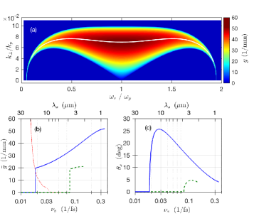
Figure 2: Plane wave amplification in CaF₂ crystal with $n_{2}=2\times 10^{-16}$ cm²/W; $I_{p}=50$ TW/cm². (a) g versus $\omega_{s}/\omega_{p}$ and $k_{\!\perp}/k_{p}$; $\lambda_{p}=0.85\,\mu$m; white line indicates $\bar{k}_{\!\perp}$. (b) Maximum gain $\bar{g}=g(\bar{k}_{\!\perp})$ versus $\nu_{s}$ (bottom) and $\lambda_{s}$ (top); red dotted line represents absorption. (b)-(c) $\lambda_{p}=0.85,2.1\,\mu$m corresponds to blue full, green dashed curves, respectively. (c) $\theta_{s}$ from Eq. (13) versus $\nu_{s}$ and $\lambda_{s}$.

In Fig. 2(a) the intensity gain profile $g$ from Eq. (7b) is plotted versus $\omega_{s}/\omega_{p}$ and $k_{\!\perp}/k_{p}$; the full white line represents $\bar{k}_{\!\perp}$; pump wavelength $\lambda_{p}=2\pi c/\omega_{p}=0.85\,\mu$m and pump intensity is $I_{p}=50$ TW/cm². The validity of the analytical results has been tested by comparison to a numerical solution of wave equation (2); they are found to be in excellent agreement. Amplification occurs over a wide spectral range from $0.45-15\,\mu$m. Gain terminates along two curves which are defined by the relation discussed below Eq. (10).

In Fig. 2(b) the maximum gain $\bar{g}$ is shown on the infrared side versus seed frequency $\nu_{s}$ (bottom axis) and seed wavelength $\lambda_{s}$ (top axis); the two pump wavelengths $\lambda_{p}=0.85,2.1\,\mu$m correspond to the blue full and green dashed curves, respectively in 2(b) and (c). Maximum gain reaches a global maximum when pump and seed frequency are equal and drops towards longer wavelengths. Further, $\bar{g}$ increases with pump frequency. For $\lambda_{p}=0.85\,\mu$m the gain is still substantial at $\lambda_{s}=15\,\mu$m; amplification ($\exp(\bar{g}l)$) by more than 4 orders of magnitude can be obtained in a $l=0.5$ mm long crystal. Note that gain and absorption balance each other at $\lambda_{s}=20\,\mu$m. As a result, the medium becomes transparent in the presence of the pump beam. For $\lambda_{p}=2.1\,\mu$m the gain extends only over a narrow spectral interval. The reason for this behavior becomes clear from Fig. 2(c), where the angle for maximum amplification, Eq. (13), is plotted for the same two pump wavelengths.

For $\lambda_{p}=2.1\,\mu$m, $\theta_{s}$ reaches a maximum close to the pump wavelength and then drops to zero. This property arises from the functional form of $n(\omega)$. The angle $\theta_{s}$ depends on $\bar{k}_{\!\perp}$ which depends on $\kappa_{\!\perp}^{2}\propto\sigma^{2}-1\approx n_{n}/n_{p}^{2}+(2/n_{p})(\eta_{g}+\eta_{u}\Omega_{s}/\omega_{p})$. Depending on the material and $\lambda_{p}$, the two terms $\eta_{g}$ and $\eta_{u}\Omega_{s}/\omega_{p}$ can have opposite or equal signs. In this particular case, they are of opposite sign and comparable magnitude, so that for decreasing $\nu_{s}$, $\kappa_{\perp}^{2}$ becomes negative. From Eqs. (8) and (9) we see that then $\bar{k}_{\!\perp}=\bar{g}=0$ so that both gain and $\theta_{s}$ become zero. A similar behavior can be seen for $\lambda_{p}=0.85\,\mu$m, however stretched out over a wider spectral interval.

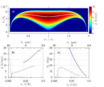
Figure 3: Plane wave amplification in KBr crystal with $n_{2}=6\times 10^{-16}$ cm²/W; $I_{p}=8$ TW/cm². (a) g versus $\omega_{s}/\omega_{p}$ and $k_{\!\perp}/k_{p}$; $\lambda_{p}=2.1\,\mu$m; white line indicates $\bar{k}_{\!\perp}$. (b) Maximum gain $\bar{g}$ versus $\nu_{s}$ (bottom) and $\lambda_{s}$ (top); red dotted line represents absorption. (b)-(c) $\lambda_{p}=0.85,2.1\,\mu$m corresponds to blue full, green dashed lines, respectively. (c) $\theta_{s}$ from Eq. (13) versus $\nu_{s}$ and $\lambda_{s}$.

In Fig. 3, the results for a KBr crystal are shown for a pump intensity $I_{p}=8$ TW/cm²; same line styles as in Fig. 2 are used. The intensity gain profile $g$ in Fig. 3(a) is plotted for $\lambda_{p}=2.1\,\mu$m. In contrast to CaF₂, in KBr, $\lambda_{p}=2.1\,\mu$m works very well and gain extends up to twice the transmission window, see also Fig. 3(b). The maximum gain is still substantial at the edge of the transmission window, see the red dotted line. There amplification of more than four orders of magnitude can be achieved over a crystal length $l=2$ mm. For $\lambda_{p}=0.85\,\mu$m, the gain is confined to a narrower spectral range (up to $8\,\mu$m). The reason becomes clear from Fig. 3(c).

For $\lambda_{p}=0.85\,\mu$m, the angle rises sharply for increasing seed wavelength. This comes from the fact that both terms in $\sigma^{2}-1$ carry the same sign. Here, the gain terminates when the denominator in Eq. (7b) goes to zero for $k_{p}=\sigma D_{u}$. By contrast for $\lambda_{p}=2.1\,\mu$m, the signs are again different and we see a similar behavior as in Fig. 2(c). Clearly, $n(\omega)$ strongly influences KIA and therefore presents a critical design parameter.

4 Kerr instability amplification of finite pulses

In extension of our plane wave analysis above, we explore KIA of finite pulses in a noncollinear setup with seed and pump pulses inclined at the optimum gain angle $\theta_{\rm s}$. We also expect KIA of Bessel-Gaussian seed pulses to work well, as the KIA profile is of Bessel-Gaussian nature. This will be subject to future research.

4.1 Theory

Our analysis relies on assuming a pump plane wave. This is justified, as long as the pump pulse is wider than the seed pulse so that its intensity varies weakly over the seed pulse. The seed pulse is assumed to be inclined at $\theta_{\rm s}$ along $x$ with a Gaussian spatial and temporal profile and field strength $E_{s}$; the spatial and temporal $1/e^{2}$-widths are $\mathrm{w}_{x}(0)=\mathrm{w}_{x}=2/\Delta_{x}$, $\mathrm{w}_{y}(0)=\mathrm{w}_{y}=2/\Delta_{y}$ and $\tau=\tau(0)$, respectively. The initial Gaussian seed pulse in the Fourier domain is given by

$$\tilde{v}_{x}(0)={2^{3/2}E_{s}f(\Omega)\over\Delta_{x}\Delta_{y}\Delta_{\omega}}\exp\left(-\left(\frac{k_{x}-\bar{k}_{\perp s}}{\Delta_{x}}\right)^{2}-\left(\frac{k_{y}}{\Delta_{y}}\right)^{2}\right)\text{,}$$ (14)

where $f=\exp(-(\Omega-\Omega_{s})^{2}/\Delta_{\omega}^{2})$ with $\Delta_{\omega}(0)=\Delta_{\omega}=2/\tau$. As the transverse wavevector of maximum amplification $\bar{k}_{\!\perp}(\Omega)$ varies as a function of frequency, (transverse) beam center and amplification maximum move increasingly apart with growing $|\Omega-\Omega_{s}|$. In the strong amplification limit the transverse beam center will align with the amplification maximum, resulting in an angular chirp [20], i.e. different frequency components have slightly different transverse wavevector centers. The amplified pulse spectrum can be approximately evaluated analytically by Taylor expanding the gain $g$ about $\bar{k}_{\!\perp}(\Omega)$; to leading order this results in a Gaussian intensity amplification profile, where

$$g\approx\bar{g}-g_{2}\,(k_{x}-\bar{k}_{\!\perp})^{2}\text{,}\,\,\,\,\,\,g_{2}={2k_{p}\bar{k}_{\!\perp}^{2}\over\delta_{\!\perp}^{2}(k_{p}^{2}-(\sigma D_{u})^{2})}\text{.}$$ (15)

The gain only modifies the $k_{x}$ pulse profile. Together with Eq. (7a) we obtain the Fourier beam amplitude after amplifier length $l$

$$\tilde{v}_{x}(\mathbf{k}_{\perp},l,\Omega)=\tilde{v}_{x}(0)\exp\left(-i\sigma D_{u}l+\frac{1}{2}\bar{g}l\right)\exp\left(-\frac{i}{2}\alpha lk_{y}^{2}\right)$$

$$\times\exp\left(-\frac{l}{2}(g_{2}+i\alpha)(k_{x}-\bar{k}_{\perp})^{2}-i\alpha l\bar{k}_{\perp}(k_{x}-\bar{k}_{\perp})\right)\text{,}$$ (16)

where $\alpha(\Omega)=\sigma D_{u}/(k_{p}^{2}-(\sigma D_{u})^{2})$. Propagation in free space after the amplifier for a length $l_{1}$ is not considered here; it can be accounted for by multiplying Eq. (16) with the factor $\exp\{-il_{1}[k(\Omega)-(1/2)k_{\!\perp}^{2}/k(\Omega)]\}$.

Inverse Fourier transform with regard to $\mathbf{k}_{\perp}$ gives a complex shifted Gaussian beam

$$\tilde{v}_{x}(x,y,l,\Omega) =\frac{E_{s}\tau\mathrm{w}_{x}\mathrm{w}_{y}}{\sqrt{2q_{x}q_{y}}}f(\Omega)\exp\left(({\gamma\over 2}-i\varkappa)l+i\bar{k}_{\!\perp s}x\right)$$

$$\times\exp\left(-{(x-x_{c})^{2}\over q_{x}}-{y^{2}\over q_{y}}\right)\text{}$$ (17)

with $\gamma=\bar{g}-g_{2}\,(\bar{k}_{\!\perp}-\bar{k}_{\!\perp s})^{2}$ and $\varkappa=\sigma D_{u}-(\alpha/2)(\bar{k}_{\!\perp}^{2}-\bar{k}_{\!\perp s}^{2})$; further, $q_{x}=\mathrm{w}_{x}^{2}+2(g_{2}+i\alpha)l$, $q_{y}=\mathrm{w}_{y}^{2}+2i\alpha l$ are related to the $1/e^{2}$-beam widths via $\mathrm{w}^{2}_{x,y}(l)=|q_{x,y}|^{2}/\mathrm{Re}(q_{x,y})$, and the complex shift of beam center is given by $x_{c}=x_{cr}+ix_{ci}=\alpha l\bar{k}_{\!\perp s}+ig_{2}l\,\left(\bar{k}_{\!\perp}-\bar{k}_{\!\perp s}\right)$. We use the following notation; subscript, $s$, denotes ($\Omega_{s}$); otherwise the argument is ($\Omega$).

From Eq. (17) the intensity spectrum follows as

$$|\tilde{v}_{x}(x,y,l,\Omega)|^{2} =\frac{(E_{s}\tau\mathrm{w}_{x}\mathrm{w}_{y})^{2}}{2|q_{x}q_{y}|}|f(\Omega)|^{2}\exp\left(\Gamma l\right)$$

$$\times\exp\left(-{2(x-\xi_{cr})^{2}\over\mathrm{w}_{x}^{2}(l)}-{2y^{2}\over\mathrm{w}_{y}^{2}(l)}\right)\text{.}$$ (18)

Due to contributions from the imaginary parts in the exponent of (17) the shift of the beam center changes to $\xi_{cr}=x_{cr}+x_{ci}(\mathrm{Im}(q_{x})/\mathrm{Re}(q_{x}))$; the gain changes to $\Gamma=\bar{g}-g_{2}\,(\bar{k}_{\!\perp}-\bar{k}_{\!\perp s})^{2}(\mathrm{w}_{x}^{2}/\mathrm{Re}(q_{x}))$. Taylor expansion of the gain about $\Omega_{s}$ yields $\Gamma(\Omega)=\Gamma_{s}+\Gamma^{\,\prime}_{s}(\Omega-\Omega_{s})+(1/2)\,\Gamma^{\,\prime\prime}_{s}(\Omega-\Omega_{s})^{2}$. As a result, the amplified spectrum remains Gaussian. Integration over $\Omega$ by using the method of stationary phase results in a spectral $1/e^{2}$-width $\Delta_{\omega}(l)=2/\tau_{g}(l)$. Here, $\tau_{g}(l)=(\tau^{2}-\Gamma^{\,\prime\prime}_{s}l)^{1/2}$ is the gain modified temporal $1/e^{2}$-duration which corresponds to the actual pulse duration $\tau(l)$ when dispersive effects are small. Finally, integration over transverse coordinates yields the amplified seed pulse energy

$$\frac{W_{s}(l)}{W_{s}(0)}=\frac{\mathrm{w}_{x}}{\sqrt{\mathrm{Re}[q_{x}(\Omega_{s})]}}\frac{\tau}{\tau_{g}(l)}\exp\left(\Gamma_{s}l+\frac{(\Gamma^{\,\prime}_{s}l)^{2}}{2\tau_{g}^{2}(l)}\right)\text{,}$$ (19)

where $W_{s}(0)=(\pi/2)^{3/2}I_{s}\tau\mathrm{w}_{x}\mathrm{w}_{y}$ and $I_{s}$ are the initial seed pulse energy and intensity. The spatio-temporal profile could also be calculated by Taylor expanding the exponent in Eq. (17) to second order in $\Omega$ followed by an inverse Fourier transform. Due to the onerous complexity this is not done here. Instead spatio-temporal profiles and $\tau(l)$ are determined numerically from Eq. (17).

4.2 Results

KIA operates in the limit where the amplified seed intensity is small compared to the pump peak intensity, so that nonlinear terms in Eq. (1) are negligible. This is fulfilled for $I_{s}(l)=I_{p}/10$ [13]. The corresponding amplified seed pulse energy is $W_{s}(l)=(\pi/2)^{3/2}I_{s}(l)\tau(l)\mathrm{w}_{x}(l)\mathrm{w}_{y}(l)$, from which together with Eq. (19) the initial pulse energy and intensity are obtained.

Efficient amplification requires the seed pulse to stay close to the pump pulse center over the whole amplification distance. This requirement sets a lower limit for pump pulse duration and width, and thereby for the minimum pump energy.

There are four factors that cause an increase in pump energy requirements: i) the inclination between pump and seed pulse axes, resulting in a walk-off $\xi_{cr}$ between beam centers; ii) widening of the seed beam widths $\mathrm{w}_{x,y}(l)$ due to diffraction and transverse spectral gain narrowing; iii) a temporal walk-off, $\Delta\beta_{1}l$, caused by the difference $\Delta\beta_{1}=\beta_{1s}-\beta_{1}$ between seed group velocity $\beta_{1s}=[dK_{u}/d\Omega](\Omega_{s})$ and pump group velocity $\beta_{1}$ defined below Eq. (4); iv) lengthening of the seed pulse duration $\tau(l)$ due to spectral gain narrowing and dispersive effects.

These 4 conditions determine the required pump pulse parameters as $\mathrm{w}_{p}=r(\mathrm{w}_{x}(l)+0.5\xi_{cr})$ and $\tau_{p}=r(\tau(l)+0.5|\Delta\beta_{1}|l)$; the factor $1/2$ comes from the assumption that pump and seed beam centers are aligned at half of the material length; we chose the factor by which the pump beam is wider than the final shifted seed beam as $r=3$ [13]. As a result, the minimum pump energy for KIA to operate efficiently is $W_{p}=(\pi/2)^{3/2}I_{p}\tau_{p}\mathrm{w}^{2}_{p}$ assuming a radially symmetric transverse pump beam.

Furthermore, the pump beam radius underlies another restriction; it needs to be wide enough to avoid self focusing. We determine $\mathrm{w}_{p}$ from the requirement that the material length $l=l_{sf}/5$, where $l_{sf}=\mathrm{w}_{p}(n_{p}/(2n_{n}))^{1/2}$ is the distance for critical self focusing [22]. The initial seed beam width $\mathrm{w}_{x}$ is determined from a solution of

$$l_{sf}\sqrt{2n_{n}\over n_{p}}=\mathrm{w}_{p}=r(\mathrm{w}_{x}(l)+0.5\xi_{cr})$$ (20)

with $\mathrm{w}_{x}(l)$ defined below Eq. (17); further, we assume $\mathrm{w}_{y}=\mathrm{w}_{x}$. Additional parameters to be considered are the nonlinear length $l_{n}=2k_{p}/k_{n}^{2}=2n_{p}c/(n_{n}\omega_{p})$ and dispersive length $l_{d}=2\tau_{p}^{2}/\beta_{2}$ of the pump pulse. In the limit of strong KIA the nonlinear length is shorter than the material length. As a result, $l_{d}\gg l$ to avoid pump pulse stretching through the combined action of nonlinear phase modulation and dispersion.

Finally, to keep amplification lengths short it is desirable to use high pump intensities. The obvious limit is the material damage threshold intensity $I_{th}=(2/\pi)^{1/2}F_{th}/\tau_{p}$ with $F_{th}$ the damage threshold fluence.

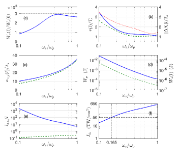
Figure 4: KIA of single cycle pulse $\tau(0)=T_{s}=2\pi/\omega_{s}$ in CaF₂; $n_{2}=2\times 10^{-16}$ cm²/W; $I_{p}=50$ TW/cm², $\lambda_{p}=0.85\,\mu$m, $l=8/\bar{g}$; $\mathrm{w}_{p}$ and $\tau_{p}$, see text above Eq. (20); $\mathrm{w}_{x}(0)=\mathrm{w}_{y}(0)$ is determined from Eq. (20). (a) Seed pulse energy increase $W_{s}(l)/W_{s}(0)$ from Eq. (19) versus $\omega_{s}/\omega_{p}$; black dashed line corresponds to the cw limit $\exp(\bar{g}l)=\exp(8)\approx 3000$. (b) $\tau(l)/T_{s}$ (blue full), $\tau_{g}(l)/T_{s}$ (green, dashed), and group velocity walk off between pump and seed, $|\Delta\beta_{1}|l/T_{s}$, versus $\omega_{s}/\omega_{p}$ (red, dotted). (c) $w_{x}(l)/\lambda_{s}$ (blue, full) and $w_{y}(l)/\lambda_{s}$ (green, dashed) versus $\omega_{s}/\omega_{p}$; initial beam radius is not plotted as $w_{y}(l)\approx w_{x}(0)=w_{y}(0)$. (d) Minimum required pump energy $W_{p}$ (blue, full), see text above Eq. (20), and corresponding seed energy $W_{s}(l)$ (green, dashed) versus $\omega_{s}/\omega_{p}$. (e) dispersive length $l_{d}/l$ (blue, full) and nonlinear length $l_{n}/l$ (green, dashed) versus $\omega_{s}/\omega_{p}$. (f) Damage threshold intensity $I_{th}$ versus $\omega_{s}/\omega_{p}$; dashed lines indicate where $I_{p}=I_{th}$.

The quantitative results for finite pulse KIA in CaF₂ and KBr are shown in Figs. 4 and 5, respectively. We assume a material length $l=8/\bar{g}(\Omega_{s})$ corresponding to a plane wave amplification factor of $\exp(8)\approx 3000$; the amplifier length $l$ is changed with frequency $\omega_{s}$ to make the plane wave amplification factor constant for all frequencies. The pump peak intensities for CaF₂ and KBr are chosen $I_{p}=50$ TW/cm² and $I_{p}=8$ TW/cm², respectively. Following the results of the plane wave analysis above, we chose $\lambda_{p}=0.85\,\mu$m and $\lambda_{p}=2.1\,\mu$m for CaF₂ and KBr, respectively. The damage threshold fluence of CaF₂ and KBr in the sub-ps pulse duration regime is $F_{th}=6.7$ J/cm² and $F_{th}=3.3$ J/cm² [21], respectively; for $n_{2}$ see caption. We assume single cycle initial seed pulses with $I_{s}(l)=I_{p}/10$; initial seed pulse radius is determined from a solution of Eq. (20).

Seed pulse energy increase $W_{s}(l)/W_{s}(0)$ in Fig. 4(a) is close to the plane wave value $\exp(\bar{g}l)\approx 3000$ (black, dashed line) for $\omega_{s}/\omega_{p}\geq 0.5$ and drops from there; at $\omega_{s}/\omega_{p}=0.2$ amplification is still more than a factor of 1000.

In Fig. 4(b) the $1/e^{2}$-pulse duration $\tau(l)$ (blue, full) is obtained from transverse space integration over the spatio-temporal intensity profile; the intensity profile is calculated as the absolute square of the Fourier transform of Eq. (17). The pulse duration $\tau(l)$ is compared to $\tau_{g}(l)$ (green, dashed) which is the gain widened pulse duration defined below Eq. (18); it is obtained from the spectral width and does not contain dispersive widening. Comparison shows that up to $\omega_{s}/\omega_{p}\approx 0.3$ amplification of single cycle pulses is possible and that the influence of dispersive effects is weak; even at $\omega_{s}/\omega_{p}=0.2$ amplification of two cycle pulses is still feasible. Below that the pulse duration rises quickly due to a mixture of gain and dispersive widening. Finally, the red dotted line indicates the shift between peak of seed and pump pulse due to group velocity mismatch.

Widening of the seed beam radius is not dramatic, as can be seen in Fig. 4(c). This is due to the fact that a large pump beam radius is required to avoid self-focusing. This results in a large seed beam radius, as in our above design considerations the seed radius increases proportional with the pump radius. In general, it is desirable to choose the seed beam radius as large as possible to optimize energy extraction from the pump beam. We find that (green, dashed) $\mathrm{w}_{y}(l)\approx\mathrm{w}_{x}(0)=\mathrm{w}_{y}(0)$ which is why the initial pulse radii are not plotted. Amplification moderately widens $\mathrm{w}_{x}(l)$ (blue, full), as defined below Eq. (17), and results in a beam asymmetry which is weak over most of the frequency range.

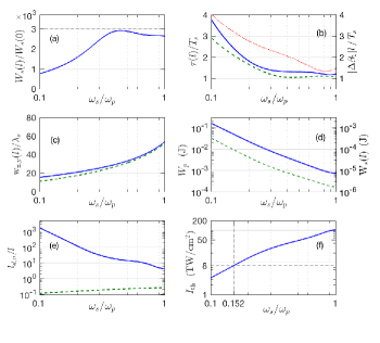
Figure 5: KIA of single cycle pulse $\tau(0)=T_{s}$ in KBr; $n_{2}=6\times 10^{-16}$ cm²/W; $I_{p}=8$ TW/cm², $\lambda_{p}=2.1\,\mu$m, $l=8/\bar{g}$; $\mathrm{w}_{p}$ and $\tau_{p}$, see text above Eq. (20); $\mathrm{w}_{x}(0)=\mathrm{w}_{y}(0)$ is determined from Eq. (20). (a) Seed pulse energy increase $W_{s}(l)/W_{s}(0)$ from Eq. (19) versus $\omega_{s}/\omega_{p}$; black dashed line corresponds to the cw limit $\exp(\bar{g}l)\approx 3000$. (b) $\tau(l)/T_{s}$ (blue full), $\tau_{g}(l)/T_{s}$ (green, dashed), and group velocity walk off between pump and seed, $|\Delta\beta_{1}|l/T_{s}$, versus $\omega_{s}/\omega_{p}$ (red, dotted). (c) $w_{x}(l)/\lambda_{s}$ (blue, full) and $w_{y}(l)/\lambda_{s}$ (green, dashed) versus $\omega_{s}/\omega_{p}$; initial beam radius is not plotted as $w_{y}(l)\approx w_{x}(0)=w_{y}(0)$. (d) Minimum required pump energy $W_{p}$ (blue, full), see text above Eq. (20), and corresponding seed energy $W_{s}(l)$ (green, dashed) versus $\omega_{s}/\omega_{p}$. (e) dispersive length $l_{d}/l$ (blue, full) and nonlinear length $l_{n}/l$ (green, dashed) versus $\omega_{s}/\omega_{p}$. (f) Damage threshold intensity $I_{th}$ versus $\omega_{s}/\omega_{p}$; dashed lines indicate where $I_{p}=I_{th}$.

In Fig. 4(d) the minimum pump pulse energy needed for KIA to work and the corresponding amplified seed pulse energy are plotted versus $\omega_{s}/\omega_{p}$. Naturally, higher seed energies can be obtained when more pump energy is available. At $\omega_{s}/\omega_{p}=0.2$ we find $W_{p}=4$ mJ which is comfortably available in Ti:sapphire laser systems. The pump energy is larger than the final seed energy by a factor of about $400-500$.
The nonlinear length $l_{n}$ (green dashed) is shorter than the amplifier length, see Fig. 4(e). The dispersive length $l_{d}$ (blue, full) is between two to four orders of magnitude longer than the medium length so that no significant pump pulse distortions are expected through the interplay of Kerr nonlinearity and group velocity dispersion.
Finally, Fig. 4(f) shows the damage threshold intensity $I_{th}$ for a pump pulse with pulse duration $\tau(l)$. The dashed line indicates the value of $\omega_{s}/\omega_{p}=0.165$ at which $I_{p}=I_{th}$. As a result, we can conclude that amplification for a wavelength range between $\lambda_{s}=0.85\,\mu$m and $\lambda_{s}\approx 5.2\,\mu$m is possible. The damage intensity presents a main limitation in extending KIA to even longer wavelengths. Reducing $I_{p}$ does not help. This results in an increase of material length $l$ to achieve the same amplification; longer $l$ results in larger $\tau(l)$, and in an enhanced walk-off, which results in turn in longer pump pulse duration $\tau_{p}$ and reduced damage threshold intensity.
Figure 5 shows the results for KBr. The results are qualitatively similar to what was found for CaF₂ in Fig. 4; therefore we focus on a discussion of Fig. 5(d) and (f). The minimum required pump energy $W_{p}\approx 20$ mJ at $\omega_{s}/\omega_{p}=0.2$. This is in the range of what can be achieved by current state of the art Ho:YAG femtosecond amplifier systems operating at wavelengths $\lambda_{p}=1.9-2.1\,\mu$m [4]. The corresponding seed amplified energy is $W_{s}\approx 50\,\mu$J. From 5(f) we find that KIA is possible for $\omega_{s}/\omega_{p}>0.152$ corresponding to a maximum seed wavelength of $\lambda_{s}\approx 14\,\mu$m.
Finally, it is interesting to look at the quality of the amplified pulses. Again our two systems behave fairly similar, which is why we show only the results for CaF₂ and $\lambda_{p}=0.85\,\mu$m; for other parameters see Fig. 4. In Fig. 6(a),(c) the spatio-spectral intensity profile $|\tilde{\varepsilon}_{x}(x,y=0,z=l,\omega)|^{2}$ is plotted for $\omega_{s}/\omega_{p}=0.2,0.4$, respectively; Figures 6(b),(d) show the corresponding spatio-temporal profiles $|\varepsilon_{x}(x,y=0,z=l,t)|^{2}$; peak values are normalized to unity. The spectrum peak is shifted off $\omega/\omega_{s}=1$ towards higher frequencies. This comes from the fact that the blue part of the seed spectrum is amplified more strongly, as for $\omega_{s}/\omega_{p}\leq 0.4$ $\bar{g}$ increases towards higher seed frequencies. Further, the spectrum exhibits some asymmetry which is not contained in the quadratic expansion of $\Gamma$ below Eq. (18); accounting for it analytically would require expansion to third order.

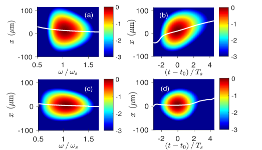
Figure 6: Spatio-spectral (a,c) and spatio-temporal (b,d) intensity profiles of seed pulses amplified in CaF₂ for $\omega_{s}/\omega_{p}=0.2,0.4$, respectively; parameters are the same as in Fig. 4; peaks are normalized to unity; time is given with reference to time $t_{0}$ of the pulse peak and normalized to the optical cycle $T_{s}$. The white lines indicate the transverse pulse maximum.

The fact that maximum gain $\bar{g}$ is experienced at finite transverse wavevector $\bar{k}_{\perp}(\Omega)$, the value of which is frequency dependent, results in a Gaussian pulse in space domain shifted by $x_{c}$, see Eq. (17). The real part of the shift $\xi_{cr}$ manifests as an off-axis shift of the pulse center, see the white line in 6(a),(c); the shift changes slightly with frequency as a result of the angular chirp, i.e. each frequency experiences optimum amplification at a slightly different angle. The angular chirp needs to be compensated, as otherwise the frequency dependent shift of the pulse center will continue growing during free space propagation [13], resulting in a degradation of the pulse quality. The imaginary part $x_{ci}$ has an effect on the spatio-temporal pulse in 6(b),(d). It creates an x-dependent group velocity component which skews the pulse in the $x-t$ plane. The pulse distortion becomes pronounced for $\omega_{s}/\omega_{p}\leq 0.2$ and is negligible for $\omega_{s}/\omega_{p}\geq 0.35$.

5 Conclusion

We have introduced a new concept for amplification of mid infrared pulses based on the Kerr instability. Our proof-of-principle theoretical analysis of KIA in CaF₂ and KBr crystals demonstrates the potential to amplify pulses in the wavelength range $\approx 1-14\,\mu$m. Whereas plane wave amplification in KBr extends to $40\mu$m, material damage limits finite pulse KIA to about $14\mu$m. There, seed pulse output energies in the $50\,\mu$J range appear feasible with a ratio of pump to seed pulse energy in the range 400-500. Our numbers are comparable to the performance of optical parametric amplifiers.
The biggest three advantages of KIA are the capacity for single cycle pulse amplification, that it is intrinsically phase matched, and its simplicity and versatility; Kerr materials are more easily available than infrared materials with second order nonlinearity. Further, amplifier wavelength can be selected by simply changing the angle between pump and seed beam. The biggest drawback is an angular chirp acquired during amplification that needs to be controlled. There exist methods to that end, from a simple prism to more sophisticated techniques [23]. Alternatively, it should also be possible to identify favorable materials that minimize the angular chirp, as the angular chirp is greatly influenced by the frequency dependence of the refractive index.
The results shown here are promising, but most likely still far from optimum. There is a huge parameter space to be explored, such as all potential infrared crystals. Further, KIA can be optimized by determining favorable optical properties (e.g. refractive index) from our theory and then designing corresponding (meta) materials. Moreover, restrictions of the amplification range arising from material damage can be mitigated by crystal cooling and parameter optimization. Finally, the KIA profile is of Bessel-Gaussian nature. Therefore KIA should lend itself naturally to the amplification of Bessel-Gauss beams.
See Supplement 1 for supporting content.

6 Supplementary Material

6.1 Limiting cases of KIA theory

In the limits of $\mathbf{k}_{\perp}=0$ and $\Omega=0$, Eq. (7b) reduces to the temporal modulation instability [11], and the spatial filamentation instability [10], respectively. For $\Omega/\omega_{p}\ll 1$ and $n_{n}\ll 1$ we can approximate $D_{u}\approx\beta_{1}\Omega$, $D_{g}\approx\beta_{2}\Omega^{2}/2$, $\sigma\approx 1$, $k_{p}^{2}-(\sigma D_{u})^{2}\approx k_{p}^{2}$, $\delta_{\!\perp}^{2}\approx k_{n}^{2}(\omega_{p})$. By using the approximation below Eq. (5) we find $\sigma^{2}-1\approx(k_{n}(\omega_{p})/k_{p})^{2}+2D_{g}/k_{p}$ and obtain

$$g\approx\sqrt{\left({k_{n}^{2}(\omega_{p})\over k_{p}}\right)^{2}-\left({k_{n}^{2}(\omega_{p})\over k_{p}}+{\beta_{2}\Omega^{2}}-{k_{\perp}^{2}\over k_{p}}\right)^{2}}\text{.}$$ (21)

By setting $\Omega=0$ in Eq. (21), a relation for the filamentation instability is obtained in agreement with [10]. By setting $k_{\perp}=0$ and by introducing the fiber nonlinear coefficient $\gamma=n_{2}\omega_{p}/(2n_{p}cA_{\rm eff})$ we can express the nonlinear term as $k_{n}^{2}(\omega_{p})/k_{p}=2\gamma P_{p}$. Here $I_{p}=P_{p}/A_{\rm eff}$, $A_{\rm eff}$ is the effective fiber pulse area, and $P_{p}$ the pump peak power. The equation resulting from Eq. (21) agrees with the gain for modulation instability in fibers [11],

$$g\approx\sqrt{(\beta_{2}\Omega^{2})^{2}+4\gamma P_{p}\beta_{2}\Omega^{2}}\text{.}$$ (22)

Finally, note that we have defined the total refractive index, $(n_{p}^{2}+n_{n})^{1/2}$, differently to Ref. [11], where $n_{p}+n_{n}$ is used; as a result $2\gamma n_{p}$ corresponds to $\gamma$ defined in Ref. [11].

6.2 Summary of definitions and parameters

In the following a summary of the definintions and variables used in this work is given. For variables defined in the text we give the equation number and use $\uparrow$ or $\downarrow$ to indicate the location of the defnition with regard to the equation number.

Location	Variable	Description
Section II
$\uparrow$(1)	$\mathbf{E}(\mathbf{x},t)$	$\mathbf{E}(\mathbf{x},t)=\boldsymbol{\varepsilon}(\mathbf{x},t)+$
		$\hat{\mathbf{x}}E_{p}\exp(i\omega_{\rm p}t-ik_{p}z)+{\rm c.c.}$
$\uparrow$(1)	${E_{p}}$	Pump electric field amplitude
$\uparrow$(1)	$\omega_{p}$	Pump angular frequency
$\downarrow$(1)	$k_{p}$	Pump wavevector
$\uparrow$(1)	$\boldsymbol{\varepsilon}(\mathbf{x},t)$	Small perturbation (seed)
$\downarrow$(1)	$n(\omega)$	Linear refractive index
$\downarrow$(1)	$n_{2}$	Optical Kerr nonlinear index
$\downarrow$(1)	$n_{n}$	$n_{n}=n_{2}I_{p}$
$\downarrow$(1)	$I_{p}$	Pump intensity
$\uparrow$(2)	$\boldsymbol{v}(\mathbf{x},t)$	$\boldsymbol{v}(\mathbf{x},t)=\boldsymbol{\varepsilon}(\mathbf{x},t)\exp(-i\omega_{\rm p}t+ik_{\rm p}z)$
$\uparrow$(2)	$\boldsymbol{k}_{\perp}$	Transverse wavevector
$\uparrow$(2)	$\tilde{\boldsymbol{v}}(z,\boldsymbol{k}_{\perp},\Omega)$	Fourier transform of $\boldsymbol{v}(\mathbf{x},t)$
$\downarrow$(2)	$k_{v}$	$k_{v}=\sqrt{k^{2}+2k_{n}}$

Location	Variable	Description
Section II
$\downarrow$(2)	$k$	$k=n(\omega)\omega/c$
$\downarrow$(2)	$k_{n}$	$k_{n}=\sqrt{n_{n}}\omega/c$
$\downarrow$(2)	$k_{\perp}^{2}$	$k_{\perp}^{2}=k_{x}^{2}+k_{y}^{2}$
$\downarrow$(2)	$\tilde{\boldsymbol{v}}_{(-)}^{*}$	$\tilde{\boldsymbol{v}}_{(-)}^{*}=\tilde{\boldsymbol{v}}^{*}(-\Omega)$
$\downarrow$(3)	$\eta$	$\eta=\sqrt{n^{2}+2n_{n}}$
$\downarrow$(3)	$\eta_{p}$	$\eta_{p}=\eta(\omega_{p})=\eta(\Omega=0)$
$\uparrow$(4)	$\Delta\eta(\Omega)$	$\Delta\eta(\Omega)=\eta(\omega_{p}+\Omega)-\eta_{p}$
$\uparrow$(4)	$\eta_{g}(\Omega)$	$\eta_{g}(\Omega)=[\Delta\eta(\Omega)+\Delta\eta(-\Omega)]/2$
$\uparrow$(4)	$\eta_{u}(\Omega)$	$\eta_{u}(\Omega)=[\Delta\eta(\Omega)-\Delta\eta(-\Omega)]/2$
(4a)	$D_{g}(\Omega)$	Even dispersion function
(4b)	$D_{u}(\Omega)$	Odd dispersion function
$\downarrow$(4)	$\beta_{1}$	$\beta_{1}=[dk/d\omega](\omega_{p})$
$\downarrow$(4)	$\beta_{2}$	$\beta_{2}=[d^{2}k/d\omega^{2}](\omega_{p})$
$\downarrow$(5)	$\sigma$	$\sigma=[k_{v}(\omega_{p})+D_{g}]/k_{p}$
$\downarrow$(5)	$\sigma^{2}-1$	$\sigma^{2}-1\approx(k_{n}(\omega_{p})/k_{p})^{2}+2D_{\rm g}/k_{\rm p}$
$\uparrow$(7)	$\kappa_{\perp}$	$\kappa_{\perp}=\sqrt{(k_{p}^{2}-D_{u}^{2})(\sigma^{2}-1)}$
$\uparrow$(7)	$K_{v}$	$K_{v}=K_{u}+K_{g}$
(7a)	$K_{u}$	$K_{u}=-\sigma D_{u}\left[1-\frac{(\kappa_{\perp}^{2}-k_{\perp})^{2}}{2(k_{p}^{2}-\sigma^{2}D_{u}^{2})}\right]$
(7b)	$K_{g}$	$K_{g}=-\frac{k_{p}\sqrt{(\kappa_{\perp}^{2}-k_{\perp})^{2}-\delta_{\perp}^{4}}}{2(k_{p}^{2}-\sigma^{2}D_{u}^{2})}$
$\uparrow$(8)	$g$	Intensity gain, $g=-2\rm{Im}(K_{g})$
(8)	$\bar{k}_{\perp}$	Transverse wavevector for max gain
(9)	$\bar{g}$	Max intensity gain
(10)	$\delta_{\perp}$	Transverse instability
		half-width
Section III
$\downarrow$(11)	$l$	Kerr material length
$\downarrow$(11)	$\bar{k}_{\perp s}$	$\bar{k}_{\perp s}=\bar{k}_{\perp}(\Omega_{s})$
$\downarrow$(12)	$\mathbf{K}(\Omega_{s})$	Instability wavevector
$\downarrow$(12)	$K_{z}$	$K_{z}=k_{p}+\sigma D_{u}$
$\downarrow$(12)	$K_{zs}$	$K_{zs}=K_{z}(\Omega_{s})$
$\downarrow$(12)	$E_{s}$	Seed electric field strength
$\downarrow$(12)	$\omega_{s}$	$\omega_{s}=\omega_{p}+\Omega_{s}$
$\downarrow$(12)	$\nu_{s}$	Seed frquency, $\nu_{s}=\omega_{s}/(2\pi)$
(13)	$\theta_{s}$	$\theta_{s}=\arctan\left(\bar{k}_{\perp s}/K_{zs}\right)$
$\downarrow$(13)	$\lambda_{p,s}$	Pump, seed wavelength

Location	Variable	Description
Section IV
$\uparrow$(14)	$\mathrm{w}_{x,y}(0)$	$1/e^{2}$ initial seed widths,
		$\mathrm{w}_{x,y}(0)=\mathrm{w}_{x,y}$
$\uparrow$(14)	$\Delta_{x,y}$	$\Delta_{x,y}=2/\mathrm{w}_{x,y}$
$\uparrow$(14)	$\tau(0)$	$1/e^{2}$ initial seed duration,
		$\tau(0)=\tau=T_{s}$
$\uparrow$(14)	$\Delta_{\omega}$	$\Delta_{\omega}=2/\tau$
(14)	$\tilde{v}_{x}(0)$	Initial Fourier-transformed
		Gaussian seed pulse
$\downarrow$(14)	$f(\Omega)$	$f(\Omega)=\exp\left(-(\Omega-\Omega_{s})^{2}/\Delta_{\omega}^{2}\right)$
(15)	$g_{2}$	$g_{2}=\frac{2k_{p}\bar{k}_{\perp}^{2}}{\delta_{\perp}^{2}(k_{p}^{2}-\sigma^{2}D_{u}^{2})}$
(16)	$\tilde{v}_{x}(\boldsymbol{k}_{\perp},l,\Omega)$	Fourier beam amplitude at $l$
$\downarrow$(16)	$\alpha$	$\alpha=\frac{\sigma D_{u}}{k_{p}^{2}-\sigma^{2}D_{u}^{2}}$
(17)	$\tilde{v}_{x}(x,y,l,\Omega)$	Amplified, shifted seed
$\downarrow$(17)	$\gamma$	$\gamma=\bar{g}-g_{2}(\bar{k}_{\perp}-\bar{k}_{\perp s})^{2}$
$\downarrow$(17)	$\varkappa$	$\varkappa=\sigma D_{u}-\alpha/2(\bar{k}_{\perp}^{2}-\bar{k}_{\perp s}^{2})$
$\downarrow$(17)	$q_{x}$	$q_{x}=\mathrm{w}_{x}^{2}+2(g_{2}+i\alpha)l$
$\downarrow$(17)	$q_{y}$	$q_{y}=\mathrm{w}_{y}^{2}+2i\alpha l$
$\downarrow$(17)	$\mathrm{w}_{x,y}(l)$	$\mathrm{w}_{x,y}(l)=\frac{\left|q_{x,y}\right|}{\sqrt{\mathrm{Re}\left(q_{x,y}\right)}}$
$\downarrow$(17)	$x_{c}$	Complex seed center,
		$x_{c}=x_{cr}+ix_{ci}$
$\downarrow$(17)	$x_{cr}$	$x_{cr}=\alpha l\bar{k}_{\perp s}$
$\downarrow$(17)	$x_{ci}$	$x_{ci}=g_{2}l(\bar{k}_{\perp}-\bar{k}_{\perp s})$
(18)	$|\tilde{v}_{x}(l)|^{2}$	Intensity spectrum of amplified
		complex-shifted Gaussian seed
$\downarrow$(18)	$\xi_{cr}$	$\xi_{cr}=x_{cr}+x_{ci}(\rm{Im}(q_{x})/\rm{Re}(q_{x}))$
$\downarrow$(18)	$\Gamma$	$\Gamma=\bar{g}-g_{2}(\bar{k}_{\perp}-\bar{k}_{\perp s})^{2}\frac{\mathrm{w}_{x}^{2}}{\mathrm{Re}(q_{x})}$
$\downarrow$(18)	${\Gamma_{s}}$	${\Gamma_{s}}={\Gamma}(\Omega_{s})$
$\downarrow$(18)	$\tau_{g}(l)$	$\tau_{g}(l)=\sqrt{\tau^{2}-\Gamma_{s}^{\prime\prime}l}$
$\downarrow$(18)	$\Delta_{\omega}(l)$	$\Delta_{\omega}(l)=2/\tau_{g}(l)$
$\uparrow$(19)	$\tau(l)$	Actual pulse duration after $l$
(19)	$W_{s}(l)$	Amplified seed pulse energy
$\downarrow$(19)	$W_{s}(0)$	Initial seed pulse energy
		$W_{s}(0)=(\pi/2)^{3/2}I_{s}\tau\mathrm{w}_{x}\mathrm{w}_{y}$
$\downarrow$(19)	$I_{s}$	Initial seed intensity
$\uparrow$(20)	$\Delta\beta_{1}$	Group velocity mismatch,
		$\Delta\beta_{1}=\beta_{1s}-\beta_{1}$
$\uparrow$(20)	wp	Pump width,
		$\mathrm{w}_{p}=r\left(\mathrm{w}_{x}(l)+0.5\xi_{cr}\right)$

Location	Variable	Description
Section IV
$\uparrow$(20)	$\tau_{p}$	Pump duration,
		$\tau_{p}=r\left(\tau(l)+0.5|\Delta\beta_{1}|l\right)$
$\uparrow$(20)	$r$	Pump to seed width ratio, $r=3$
$\uparrow$(20)	$W_{p}$	Pump energy,
		$W_{p}=(\pi/2)^{3/2}I_{p}\tau_{p}\mathrm{w}^{2}_{p}$
$\uparrow$(20)	$l_{sf}$	Self-focusing length,
		$l_{sf}=\mathrm{w}_{p}\sqrt{n_{p}/(2n_{n})}$
$\downarrow$(20)	$l_{n}$	Nonlinear length, $l_{n}=2n_{p}c/(n_{n}\omega_{p})$
$\downarrow$(20)	$l_{d}$	Dispersion length, $l_{d}=2\tau_{p}^{2}/\beta_{2}$
$\downarrow$(20)	$F_{th}$	Damage threshold fluence
$\downarrow$(20)	$I_{th}$	Damage threshold intensity,
		$I_{th}=\sqrt{2/\pi}F_{th}/\tau_{p}$

Table 1: Summary of the variables, their locations, and definitions used in this work.

References

• [1] S. Ghimire et al., Observation of high-order harmonic generation in a bulk crystal, Nature physics 7, 138 (2011).
• [2] A. Schiffrin et al. Optical-field-induced current in dielectrics, Nature 493, 70 (2013).
• [3] R. Gattass and E. Mazur, Femtosecond laser micromachining in transparent materials, Nature photonics 2, 219 (2008).
• [4] P. Malevich et al., High energy and average power femtosecond laser for driving mid-infrared optical parametric amplifiers, Opt. Lett. 38, 2746 (2013).
• [5] B. E. Schmidt et al. Frequency domain optical parametric amplification, Nature communications 5, 3643 (2014).
• [6] C. Manzoni and G. Cerullo, Design criteria for ultrafast optical parametric amplifiers, Journal of Optics 18, 103501 (2016).
• [7] P. Krogen et al., Generation and multi-octave shaping of mid-infrared intense single-cycle pulses, Nature Photonics textbf11, 222 (2017).
• [8] A. Couairon, A. Mysyrowicz, Femtosecond filamentation in transparent media, Phys. Rep. 441, 47 (2007).
• [9] M. Z. Alam, I. De Leon, R. W. Boyd, Large optical nonlinearity of indium tin oxide in its epslion-near-zero region, Science 352, 795 (2016).
• [10] V. I. Bespalov and V. I. Talanov, Filamentary structure of light beams in nonlinear liquids, JETP Lett. 3, 307 (1966).
• [11] G. Agrawal, Nonlinear fiber optics, 5th edition, Academic Press (2012).
• [12] see supplementary material
• [13] G. Vampa et al., The ultimate laser amplifier, in preparation 2017.
• [14] E. D. Palik, Handbook of optical constants of solids II, Academic Press, Boston (1991).
• [15] D. Milam, M. J. Weber, and A. J. Glass, Nonlinear refractive index of fluoride crystals, Appl. Phys. Lett. 31, 822 (1977).
• [16] I. H. Malitson, A redetermination of some optical properties of calcium fluoride, App. Opt. 2, 1103 (1963).
• [17] R. DeSalvo, A. A. Said, D. J. Hagan, A. W. Van Stryland, and M. Sheik Bahae, Infrared to ultraviolet measurement of two-photon abosrption and $n_{2}$ in wide bandgap solilds, IEEE J. Quantum Electr. 32, 1324 (1996).
• [18] H. H. Li, Refractive index of alkali halides and its wavelength and temperature derivatives, J. Phys. Chem. Ref. Data 5, 329 (1976).
• [19] M. Sheik-Bahae, D. C. Hutchings, D. J. Hagan, E. W. Van Stryland, Dispersion of bound electronic nonlinear refraction in solids, IEEE J. Quant. Electr. 27, 1269 (1991)
• [20] X.Gu, S. Akturk, R. Trebino, Spatial chirp in ultrafast optics, Opt. Commun. 242, 599 (2004).
• [21] L. Gallais and M. Commadre, Laser-induced damage thresholds of bulk and coating optical materials at 1030 nm, 500 fs, Appl. Opt. 53, A186 (2014).
• [22] R. W. Boyd, Nonlinear Optics, Third edition, Academic Press, Amsterdam 2008.
• [23] O. Mendoza-Yero, G. Minguez-Vega, J. Lanzis, and V. Climent, Diffractive pulse shaper for arbitrary waveform generation, Opt. Lett. 35, 535 (2010).