Convolutional Neural Network with Word Embeddings for
Chinese Word Segmentation

Abstract

Character-based sequence labeling framework is flexible and efficient for Chinese word segmentation (CWS). Recently, many character-based neural models have been applied to CWS. While they obtain good performance, they have two obvious weaknesses. The first is that they heavily rely on manually designed bigram feature, i.e. they are not good at capturing n-gram features automatically. The second is that they make no use of full word information. For the first weakness, we propose a convolutional neural model, which is able to capture rich $n$-gram features without any feature engineering. For the second one, we propose an effective approach to integrate the proposed model with word embeddings. We evaluate the model on two benchmark datasets: PKU and MSR. Without any feature engineering, the model obtains competitive performance — 95.7% on PKU and 97.3% on MSR. Armed with word embeddings, the model achieves state-of-the-art performance on both datasets — 96.5% on PKU and 98.0% on MSR, without using any external labeled resource.

1 Introduction

Unlike English and other western languages, most east Asian languages, including Chinese, are written without explicit word delimiters. However, most natural language processing (NLP) applications are word-based. Therefore, word segmentation is an essential step for processing those languages. CWS is often treated as a character-based sequence labeling task Xue et al. (2003); Peng et al. (2004). Figure 1 gives an intuitive explaination. Linear models, such as Maximum Entropy (ME) Berger et al. (1996) and Conditional Random Fields (CRF) Lafferty et al. (2001), have been widely used for sequence labeling tasks. However, they often depend heavily on well-designed hand-crafted features.

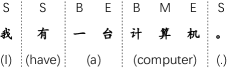
Figure 1: Chinese word segmentation as a sequence labeling task. This figure presents the common BMES (Begining, Middle, End, Singleton) tagging scheme.

Recently, neural networks have been widely used for NLP tasks. Collobert et al. (2011) proposed a unified neural architecture for various sequence labeling tasks. Instead of exploiting hand-crafted input features carefully optimized for each task, their system learns internal representations automatically. As for CWS, there are a series of works, which share the main idea with Collobert et al. (2011) but vary in the network architecture. In particular, feed-forward neural network Zheng et al. (2013), tensor neural network Pei et al. (2014), recursive neural network Chen et al. (2015a), long-short term memory (LSTM) Chen et al. (2015b), as well as the combination of LSTM and recursive neural network Xu and Sun (2016) have been used to derive contextual representations from input character sequences, which are then fed to a prediction layer.

Despite of the great success of above models, they have two weaknesses. The first is that they are not good at capturing n-gram features automatically. Experimental results show that their models perform badly when no bigram feature is explicitly used. One of the strengths of neural networks is the ability to learn features automatically. However, this strength has not been well exploited in their works. The second is that they make no use of full word information. Full word information has shown its effectiveness in word-based CWS systems Andrew (2006); Zhang and Clark (2007); Sun et al. (2009). Recently, Liu et al. (2016); Zhang et al. (2016) utilized word embeddings to boost performance of word-based CWS models. However, for character-based CWS models, word information is not easy to be integrated.

For the first weakness, we propose a convolutional neural model, which is also character-based. Previous works have shown that convolutional layers have the ablity to capture rich n-gram features Kim et al. (2016). We use stacked convolutional layers to derive contextual representations from input sequence, which are then fed into a CRF layer for sequence-level prediction. For the second weakness, we propose an effective approach to incorporate word embeddings into the proposed model. The word embeddings are learned from large auto-segmented data. Hence, this approach belongs to the category of semi-supervised learning.

We evaluate our model on two benchmark datasets: PKU and MSR. Experimental results show that even without the help of explicit $n$-gram feature, our model is capable of capturing rich n-gram information automatically, and obtains competitive performance — 95.7% on PKU and 97.3% on MSR (F score). Furthermore, armed with word embeddings, our model achieves state-of-the-art performance on both datasets — 96.5% on PKU and 98.0% on MSR, without using any external labeled resource.

2 Architecture

In this section, we introduce the architecture from bottom to top.

2.1 Lookup Table

The first step to process a sentence by deep neural networks is often to transform words or characters into embeddings Bengio et al. (2003); Collobert et al. (2011). This transformation is done by lookup table operation. A character lookup table $M_{char}\in\mathbb{R}^{|V_{char}|\times d}$ (where $|V_{char}|$ denotes the size of the character vocabulary and $d$ denotes the dimension of embeddings) is associated with all characters. Given a sentence $\mathcal{S}=(c_{1},c_{2},...,c_{L})$, after the lookup table operation, we obtain a matrix $X\in\mathbb{R}^{L\times d}$ where the $i$’th row is the character embedding of $c_{i}$.

Besides the character, other features can be easily incorporated into the model (we shall see word feature in section 3). We associate to each feature a lookup table (some features may share the same lookup table) and the final representation is calculated as the concatenation of all corresponding feature embeddings.

2.2 Convolutional Layer

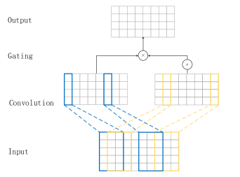
Figure 2: Structure of a convolutional layer with GLU. There are five input channels and four output channels in this figure.

Many neural network models have been explored for CWS. However, experimental results show that they are not able to capure $n$-gram information automatically Pei et al. (2014); Chen et al. (2015a, b). To achieve good performance, $n$-gram feature must be used explicitly. To overcome this weakness, we use convolutional layers Waibel et al. (1989) to encode contextual information. Convolutional neural networks (CNNs) have shown its great effectiveness in computer vision tasks Krizhevsky et al. (2012); Simonyan and Zisserman (2014); He et al. (2016). Recently, Zhang et al. (2015) applied character-level CNNs to text classification task. They showed that CNNs tend to outpeform traditional $n$-gram models as the dataset goes larger. Kim et al. (2016) also observed that character-level CNN learns to differentiate between different types of $n$-grams — prefixes, suffixes and others, automatically.

Our network is quite simple — only convolutional layers is used (no pooling layer). Gated linear unit (GLU) Dauphin et al. (2016) is used as the non-linear unit in our convolutional layer, which has been shown to surpass rectified linear unit (ReLU) on the language modeling task. For simplicity, GLU can also be easily replaced by ReLU with performance slightly hurt (with roughly the same number of network parameters). Figure 2 shows the structure of a convolutional layer with GLU. Formally, we define the number of input channels as $N$, the number of output channels as $M$, the length of input as $L$ and kernel width as $k$. The convolutional layer can be written as

$$F(X)=(X*W+b)\otimes\sigma(X*V+c)$$

where $*$ denotes one dimensional convolution operation, $X\in\mathbb{R}^{L\times N}$ is the input of this layer, $W\in\mathbb{R}^{k\times N\times M}$, $b\in\mathbb{R}^{M}$, $V\in\mathbb{R}^{k\times N\times M}$, $c\in\mathbb{R}^{M}$ are parameters to be learned, $\sigma$ is the sigmoid function and $\otimes$ represents element-wise product. We make $F(X)\in\mathbb{R}^{L\times M}$ by augmenting the input $X$ with paddings.

A succession of convolutional layers are stacked to capture long distance information. From the perspective of each character, information flows in a pyramid. Figure 3 shows a network with three convolutional layers stacked. On the topmost layer, a linear transformation is used to transform the output of this layer to unnormalized label scores $E\in\mathbb{R}^{L\times C}$, where $C$ is the number of label types.

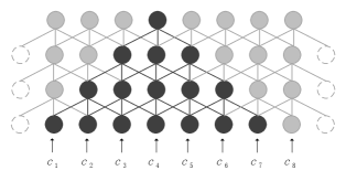
Figure 3: Stacked convolutional layers. There is one input layer on the bottom and three convolutional layers on the top. Dashed white circles denote paddings. Black circles and lines mark the pyramid in the perspective of $c_{4}$.

2.3 CRF Layer

For sequence labeling tasks, it is often beneficial to explicitly consider the correlations between adjacent labels Collobert et al. (2011).

Correlations between adjacent labels can be modeled as a transition matrix $T\in\mathbb{R}^{C\times C}$. Given a sentence $\mathcal{S}=(c_{1},c_{2},...,c_{L})$, we have corresponding scores $E\in\mathbb{R}^{L\times C}$ given by the convolutional layers. For a label sequence $y=(y_{1},y_{2},...,y_{L})$, we define its unnormalized score to be

$$s(\mathcal{S},y)=\sum\limits_{i=1}^{L}{E_{i,y_{i}}}+\sum_{i=1}^{L-1}{T_{y_{i},y_{i+1}}}.$$

then the probability of the label sequence is defined as

$$P(y|\mathcal{S})=\frac{e^{s(\mathcal{S},y)}}{\sum_{y\prime\in\mathcal{Y}}e^{s(\mathcal{S},y\prime)}}$$

where $\mathcal{Y}$ is the set of all valid label sequences. This actually takes the form of linear chain CRF Lafferty et al. (2001). Then the final loss of the proposed model is defined as the negative log-likehood of the ground-truth label sequence $y^{*}$

$$\mathcal{L}(\mathcal{S},y^{\star})=-logP(y^{\star}|\mathcal{S}).$$

During training, the loss function is minimized by back propagation. During test, Veterbi algorithm is applied to quickly find the label sequence with maximum probability.

3 Integration with Word Embeddings

Character-based CWS models have the superiority of being flexible and efficient. However, full word information is not easy to be incorporated. There is another type of CWS models: the word-based models. Models belong to this category utilize not only character-level information, but also word-level Zhang and Clark (2007); Andrew (2006); Sun et al. (2009). Recent works have shown that word embeddings learned from large auto-segmented data lead to great improvements in word-based CWS systems Liu et al. (2016); Zhang et al. (2016). We propose an effective approach to integrate word embeddings with our character-based model. The integration brings two benefits. On the one hand, full word information can be used. On the other hand, large unlabeled data can be better exploited.

Length	Features
1	$\underline{c_{i}}$
2	$c_{i-1}\underline{c_{i}}\quad\underline{c_{i}}c_{i+1}$
3	$c_{i-2}c_{i-1}\underline{c_{i}}\quad c_{i-1}\underline{c_{i}}c_{i+1}\quad\underline{c_{i}}c_{i+1}c_{i+2}$
4	$c_{i-3}c_{i-2}c_{i-1}\underline{c_{i}}\quad c_{i-2}c_{i-1}\underline{c_{i}}c_{i+1}$
	$c_{i-1}\underline{c_{i}}c_{i+1}c_{i+2}\quad\underline{c_{i}}c_{i+1}c_{i+2}c_{i+3}$

Table 1: Word features at position $i$ given a sentence $\mathcal{S}=(c_{1},c_{2},...,c_{L})$. Only the words that include the current character $c_{i}$ (marked with underline) are considered as word feature. Hence, the number of features can be controlled in a reasonable range. We also restrict the max length of words to 4 since few words contain more than 4 characters in Chinese. Note that the feature space is still tremendous ($O(N^{4})$, where $N$ is the number of characters).

To use word embeddings, we design a set of word features, which are listed in Table 1. We associate to the word features a lookup table $M_{word}$. Then the final representation of $c_{i}$ is defined as

$$\begin{split}R(c_{i})=&M_{char}[c_{i}]\oplus\\ &M_{word}[c_{i}]\oplus M_{word}[c_{i-1}c_{i}]\oplus\dots\oplus\\ &M_{word}[c_{i}c_{i+1}c_{i+2}c_{i+3}]\end{split}$$

where $\oplus$ denotes the concatenation operation. Note that the max length of word features is set to 4, therefore the feature space is extremely large ($O(N^{4})$). A key step is to shrink the feature space so that the memory cost can be confined within a feasible scope. In the meanwhile, the problem of data sparsity can be eased. The solution is as following. Given the unlabeled data $\mathcal{D}_{un}$ and a teacher CWS model, we segment $\mathcal{D}_{un}$ with the teacher model and get the auto-segmented data $\mathcal{D}_{un}^{\prime}$. A vocabulary $V_{word}$ is generated from $\mathcal{D}_{un}^{\prime}$ where low frequency words are discarded . We replace $M_{word}[*]$ with $M_{word}[\emph{UNK}]$ if $*\notin V_{word}$ (UNK denotes the unknown words).

To better exploit the auto-segmented data $\mathcal{D}_{un}^{\prime}$, we adopt an off-the-self tool word2vec Mikolov et al. (2013) to pretrain the word embeddings. The whole procedure is summarized as following setps:

1. Train a teacher model that does not rely on word feature.

2. Segment unlabeled data $\mathcal{D}$ with the teacher model and get the auto-segmented data $\mathcal{D}^{\prime}$.

3. Build a vocabulary $V_{word}$ from $\mathcal{D}^{\prime}$. Replace all words not appear in $V_{word}$ with UNK.

4. Pretrain word embeddings on $\mathcal{D}^{\prime}$ using word2vec.

5. Train the student model with word feature using the pretrained word embeddings.

Note that no external labeled data is used in this procedure.

4 Experiments

4.1 Settings

Datasets We evaluate our model on two benchmark datasets, PKU and MSR, from the second International Chinese Word Segmentation Bakeoff Emerson (2005). Both datasets are commonly used by previous state-of-the-art models. For both datasets, last 10% of the training data are used as development set. The unlabeled data used in this work is news data collected by Sogou .

We do not perform any preprocessing for these datasets, such as replacing continuous digits and English characters with a single token.

Dropout Dropout Srivastava et al. (2014) is a very efficient method for preventing overfit, especially when the dataset is small. We apply dropout to our model on all convolutional layers and embedding layers. The dropout rate is fixed to 0.2.

Hyper-parameters For both datasets, we use the same set of hyper-parameters, which are presented in Table 2. For all convolutional layers, we just use the same number of channels. Following the practice of designing very deep CNN in computer vision Simonyan and Zisserman (2014), we use a small kernal width, i.e. 3, for all convolutional layers. To avoid computational inefficiency, we use a relatively small dimension, i.e. 50, for word embeddings.

Hyper-parameters	Value
dimension of character embedding	200
dimension of word embedding	50
number of conv layers	5
number of channels per conv layer	200
kernel width of filters	3
dropout rate	0.2

Table 2: Hyper-parameters we choose for our model.

Models	PKU			MSR
	P	R	F	P	R	F
Tseng (2005)	94.6	95.4	95.0	96.2	96.6	96.4
Zhang and Clark (2007)	-	-	94.5	-	-	97.2
Zhao and Kit (2011)	-	-	95.40	-	-	97.58
Sun et al. (2012)	95.8	94.9	95.4	97.6	97.2	97.4
Zhang et al. (2013)	96.5	95.8	96.1	-	-	97.45
Pei et al. (2014)	-	-	95.2	-	-	97.2
Chen et al. (2015a)∗⋄	96.5	96.3	96.4	97.4	97.8	97.6
Chen et al. (2015b)∗⋄	96.6	96.4	96.5	97.5	97.3	97.4
Cai and Zhao (2016)⋄	95.8	95.2	95.5	96.3	96.8	96.5
Liu et al. (2016)	-	-	95.67	-	-	97.58
Zhang et al. (2016)	-	-	95.7	-	-	97.7
Xu and Sun (2016)∗⋄	-	-	96.1	-	-	96.3
CONV-SEG	96.1	95.2	95.7	97.4	97.3	97.3
WE-CONV-SEG (+ word embeddings)	96.8	96.1	96.5	97.9	98.1	98.0

Table 3: Performance of our models and previous state-of-the-art models. Note that Chen et al. (2015a, b); Xu and Sun (2016) used a external Chinese idiom dictionary. To make the comparison fair, we mark them with ^∗. Chen et al. (2015a, b); Cai and Zhao (2016); Xu and Sun (2016) also preprocessed the datasets by replacing the conitinous English character and digits with a unique token. We mark them with ^⋄.

Pretraining Character embeddings and word embeddings are pretrained on unlabeled or auto-segmented data by word2vec. Since the pretrained embeddings are not task-oriented, they are fine-tuned during supervised training by normal backpropagation.

Optimization Adam algorithm Kingma and Ba (2014) is applied to optimize our model. We use default parameters given in the original paper and we set batch size to 100. For both datasets, we train no more than 100 epoches. The final models are chosen by their performance on the development set.

Weight normalization Salimans and Kingma (2016) is applied for all convolutional layers to accelerate the training procedure and obvious acceleration is observed.

4.2 Main Results

Table 3 gives the performances of our models, as well as previous state-of-the-art models. Two proposed models are shown in the table:

• CONV-SEG  It is our preliminary model without word embeddings. Character embeddings are pretrained on large unlabeled data.

• WE-CONV-SEG  On the basis of CONV-SEG, word embeddings are used. We use CONV-SEG as the teacher model (see section 3).

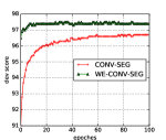
(a)

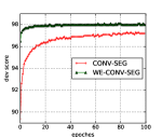
(b)

Figure 4: Learning curves (dev scores) of our models on PKU (left) and MSR (right).

Our preliminary model CONV-SEG achieves competitive performance without any feature engineering. Armed with word embeddings, WE-CONV-SEG obtains state-of-the-art performance on both PKU and MSR datasets without using any external labeled data. WE-CONV-SEG outperforms state-of-the-art neural model Zhang et al. (2016) in a large margin (+0.8 on PKU and +0.3 in MSR). Chen et al. (2015b) preprocessed all datasets by replacing Chinese idioms with a single token and thus their model obtains excellent score on PKU dataset. However, WE-CONV-SEG achieves the same performance on PKU and outperforms their model on MSR, without any data preprocessing.

We also observe that WE-CONV-SEG converges much faster compared to CONV-SEG. Figure 4 presents the learning curves of the two models. It takes 10 to 20 epoches for WE-CONV-SEG to converge while it takes more than 60 epoches for CONV-SEG to converge.

4.3 Network Depth

Network depth shows great influence on the performance of deep neural networks. A too shallow network may not fit the training data very well while a too deep network may overfit or is hard to train. We evaluate the performance of the proposed model with varying depth. Figure 5 shows the results. It is obvious that five convolutional layers is a good choise for both datasets. When we increase the depth from 1 to 5, the performance is improved significantly. However, when we increase depth from 5 to 7, even to 11 and 15, the performance is almost unchanged. This phenomenon implies that CWS rarely relies on context larger than 11 . With more training data, deeper networks may perform better.

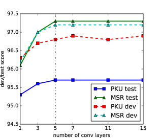
Figure 5: Scores on dev set and test set with respect to the number of convolutional layers. The vertical dashed line marks the depth we choose.

4.4 Pretraining Character Embeddings

Model Options	PKU	MSR
without pretraining	94.7	96.7
with pretraining	95.7	97.3

Table 4: Test performances with or without pretraining character embeddings. “without pretraining” means that the character embeddings are randomly initialized.

Previous works have shown that pretraining character embeddings boost the performance of neural CWS models significantly Pei et al. (2014); Chen et al. (2015a, b); Cai and Zhao (2016). We verify this and get a consistent conclusion. Table 4 shows the performances with or without pretraining. Our model obtains significant improvements (+1.0 on PKU and +0.6 on MSR) with pretrained character embeddings.

4.5 N-gram Features

Models	PKU	MSR	PKU	MSR
Cai and Zhao (2016)⋄	95.5	96.5	-	-
Zheng et al. (2013)	92.8‡	93.9‡	-	-
Pei et al. (2014)	94.0	94.9	-	-
Chen et al. (2015a)	94.5†	95.4†	96.1∗	96.2∗
Chen et al. (2015b)	94.8†	95.6†	96.0∗	96.6∗
Xu and Sun (2016)	-	-	96.1∗	96.3∗
CONV-SEG	95.7	97.3	-	-
Pei et al. (2014)	95.2	97.2	-	-
	(+1.2)	(+2.3)
Chen et al. (2015a)	-	-	96.4∗	97.6∗
			(+0.3)	(+1.4)
Chen et al. (2015b)	-	-	96.5∗	97.3∗
			(+0.5)	(+0.7)
AVEBE-CONV-SEG	95.4	97.1	-	-
	(-0.3)	(-0.2)
W2VBE-CONV-SEG	95.9	97.5	-	-
	(+0.2)	(+0.2)

Table 5: The first/second group summarize results of models without/with bigram feature. The number in the parentheses is the absolute improvement given by explicit bigram feature. Results with ^∗ used external dictionary. Results with ^† come from Cai and Zhao (2016). Results with ^‡ come from Pei et al. (2014). ^⋄ marks word-based models.

In this section, we test the ability of our model in capturing n-gram features. Since unigram is indispensable and trigram is beyond memory limit, we only consider bigram.

Bigram feature has shown to play a vital role in character-based neural CWS models Pei et al. (2014); Chen et al. (2015a, b). Without bigram feature, previous models perform badly. Table 5 gives a summarization. Without bigram feature, our model outperforms previous character-based models in a large margin (+0.9 on PKU and +1.7 on MSR). Compared with word-based model Cai and Zhao (2016), the improvements are also significant (+0.2 on PKU and +0.8 on MSR).

Then we arm our model with bigram feature. The bigram feature we use is the same with Pei et al. (2014); Chen et al. (2015a, b). The dimension of bigram embedding is set to 50. Following Pei et al. (2014); Chen et al. (2015a, b), the bigram embeddings are initialized by the average of corresponding pretrained character embeddings. The result model is named AVEBE-CONV-SEG and the performance is shown in Table 5. Unexpectedly, the performance of AVEBE-CONV-SEG is worse than the preliminary model CONV-SEG that uses no bigram feature (-0.3 on PKU and -0.2 on MSR). This result is dramatically inconsistent with previous works, in which the performance is significantly improved by the method. We also observe that the training cost of AVEBE-CONV-SEG is much lower than CONV-SEG. Hence we can conclude that the inconsistency is casued by overfitting. A reasonable conjecture is that the model CONV-SEG already capture abundant bigram feature automatically, therefore the model is tend to overfit when bigram feature is explicitly added.

A practicable way to overcome overfitting is to introduce priori knowledge. We introduce priori knowledge by using bigram embeddings directly pretrained on large unlabeled data, which is simmillar with Mansur et al. (2013). We convert the unlabeled text to bigram sequence and then apply word2vec to pretrain the bigram embeddings directly. The result model is named W2VBE-CONV-SEG, and the performance is also shown in Table 5. This method leads to substantial improvements (+0.5 on PKU and +0.4 MSR) over AVEBE-CONV-SEG. However, compared to CONV-SEG, there are only slight gains (+0.2 on PKU and MSR).

All above observations verify that our proposed network has considerable superiority in capturing n-gram, at least bigram features automatically.

4.6 Word Embeddings

Word embeddings lead to significant improvements over the strong baseline model CONV-SEG. The improvements come from the teacher model and the large unlabeled data. A natural question is how much unlabeled data can lead to significant improvements. We study this by halving the unlabeled data. Figure 6 presents the results. As the unlabeled data becomes smaller, the performance remains unchanged at the beginning and then becomes worse. This demonstrates that the mass of unlabeled data is a key factor to achieve high performance. However, even with only 68MB unlabeled data, we can still observe remarkable improvements (+0.4 on PKU and MSR). We also observe that MSR dataset is more robust to the size of unlabeled data than PKU dataset. We conjecture that this is because MSR training set is larger than PKU training set.

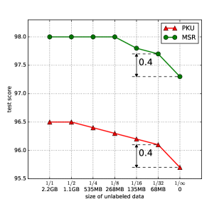
Figure 6: Test performances with varying size of unlabeled data for pretraining word embeddings. With full size, the model is WE-CONV-SEG. With the 0 size, the model degenerates to CONV-SEG.

We also study how the teacher’s performance influence the student. We train other two models that use different teacher models. One of them uses a worse teacher and the other uses a better teacher. The results are shown in Table 6. As expected, the worse teacher indeed creates a worse student, but the effect is marginal (-0.1 on PKU and MSR). And the better teacher brings no improvements. These facts demonstrate that the student’s performance is relatively insensitive to the teacher’s ability as long as the teacher is not too weak.

Models	teacher		student
	PKU	MSR	PKU	MSR
WE-CONV-SEG	95.7	97.4	96.5	98.0
worse teacher	95.4	97.1	96.4	97.9
better teacher	96.5	98.0	96.5	98.0

Table 6: Performances of student models and teacher models. A previous trained model maybe reused in following so that there are some

Not only the pretrained word embeddings, we also build a vocabulary $V_{word}$ from the large auto-segmented data. Both of them should have positive impacts on the improvements. To figure out their contributions quantitatively, we train a contrast model, where the pretrained word embeddings are not used but the word features and the vocabulary are persisted, i.e. the word embeddings are randomly initialized. The results are shown in Table 7. According to the results, we conclude that the pretrained word embeddings and the vocabulary have roughly equal contributions to the final improvements.

Models	PKU	MSR
WE-CONV-SEG	96.5	98.0
-word emb	96.1	97.6
-word feature	95.7	97.3

Table 7: Performances of our models with different word feature options. “-word emb” denotes the model in which word features and the vocabulary are used but the pretrained word embeddings are not. “-word feature” denotes the model that uses no word feature, i.e. CONV-SEG.

5 Related Work

CWS has been studied with considerable efforts in NLP commutinity. Xue et al. (2003) firstly modeled CWS as a character-based sequence labeling problem. They used a sliding-window maximum entropy classifier to tag Chinese characters into one of four position tags, and then coverted these tags into a segmentation using rules. Following their work, Peng et al. (2004) applied CRF to the problem for sequence-level prediction. Recently, under the sequence labeling framework, various neural models have been explored for CWS. Zheng et al. (2013) firstly applied a feed-forward neural network for CWS. Pei et al. (2014) improved upon Zheng et al. (2013) by explicitly modeling the interactions between local context and previous tag. Chen et al. (2015a) proposed a gated recursive neural network (GRNN) to model the combinations of context characters. Chen et al. (2015b) utilized Long short-term memory (LSTM) to capture long distant dependencies. Xu and Sun (2016) combined LSTM and GRNN to efficiently integrate local and long-distance features.

Our proposed model is also a neural sequence labeling model. The difference from above models lies in that CNN is used to encode contextual information. CNNs have been successfully applied in many NLP tasks, such as text classification Kalchbrenner et al. (2014); Kim (2014); Zhang et al. (2015); Conneau et al. (2016), language modeling Kim et al. (2016); Pham et al. (2016); Dauphin et al. (2016), machine translation Meng et al. (2015); Kalchbrenner et al. (2016); Gehring et al. (2016). Experimental results show that the convolutional layers are capable to capture more n-gram features than previous introduced networks. Collobert et al. (2011) also proposed a CNN based seuqence labeling model. However, our model is significantly different from theirs since theirs adopt max-pooling to encode the whole sentence into a fixed size vector and use position embeddings to demonstrate which word to be tagged while ours does not. Our model is more efficient due to the sharing structure in lower layers. Contemporary to this work, Strubell et al. (2017) applied dilated CNN to named entity recognition.

The integration with word embeddings is inspired by word-based CWS models Andrew (2006); Zhang and Clark (2007); Sun et al. (2009). Most recently, Zhang et al. (2016); Liu et al. (2016); Cai and Zhao (2016) proposed word-based neural models for CWS. Particularly, Zhang et al. (2016); Liu et al. (2016) utilized word embeddings learned from large auto-segmented data, which leads to significant improvements. Different from their word-based models, we integrate word embeddings with the proposed character-based model.

Simillar to this work, Wang et al. (2011) and Zhang et al. (2013) also enhanced character-based CWS systems by utilizing auto-segmented data. However, they didn’t use word embeddings, but only used statistics features. Sun (2010) and Wang et al. (2014) combined character-based and word-based CWS model via bagging and dual decomposition respectively and achieved better performance than single model.

6 Conclusion

In this paper, we address the weaknesses of character-based CWS models. We propose a novel neural model for CWS. The model utilizes stacked convolutional layers to derive contextual representations from input sequence, which are then fed to a CRF layer for prediction. The model is capable to capture rich n-gram features automatically. Furthermore, we propose an effective approach to integrate the proposed model with word embeddings, which are pretrained on large auto-segmented data. Evaluation on two benchmark datasets shows that without any feature engineering, much better performance than previous models (also without feature engineering) is obtained. Armed with word embeddings, our model achieves state-of-the-art performance on both datasets, without using any external labeled data.

References

- Abadi et al. (2016) Martín Abadi, Ashish Agarwal, Paul Barham, Eugene Brevdo, Zhifeng Chen, Craig Citro, Greg S Corrado, Andy Davis, Jeffrey Dean, Matthieu Devin, et al. 2016. Tensorflow: Large-scale machine learning on heterogeneous distributed systems. arXiv preprint arXiv:1603.04467.
- Andrew (2006) Galen Andrew. 2006. A hybrid markov/semi-markov conditional random field for sequence segmentation. In Conference on Empirical Methods in Natural Language Processing, pages 465–472.
- Bengio et al. (2003) Yoshua Bengio, R Ducharme, jean, Pascal Vincent, and Christian Janvin. 2003. A neural probabilistic language model. Journal of Machine Learning Research, 3(6):1137–1155.
- Berger et al. (1996) Adam L Berger, Vincent J. Della Pietra, and Stephen A. Della Pietra. 1996. A maximum entropy approach to natural language processing. Computational Linguistics, 22(1):39–71.
- Cai and Zhao (2016) Deng Cai and Hai Zhao. 2016. Neural word segmentation learning for chinese. In Meeting of the Association for Computational Linguistics, pages 409–420.
- Chen et al. (2015a) Xinchi Chen, Xipeng Qiu, Chenxi Zhu, and Xuanjing Huang. 2015a. Gated recursive neural network for chinese word segmentation. In ACL (1), pages 1744–1753.
- Chen et al. (2015b) Xinchi Chen, Xipeng Qiu, Chenxi Zhu, Pengfei Liu, and Xuanjing Huang. 2015b. Long short-term memory neural networks for chinese word segmentation. In Conference on Empirical Methods in Natural Language Processing, pages 1197–1206.
- Collobert et al. (2011) Ronan Collobert, Jason Weston, L Bottou, Michael Karlen, Koray Kavukcuoglu, and Pavel Kuksa. 2011. Natural language processing (almost) from scratch. Journal of Machine Learning Research, 12(1):2493–2537.
- Conneau et al. (2016) Alexis Conneau, Holger Schwenk, Loïc Barrault, and Yann Lecun. 2016. Very deep convolutional networks for natural language processing. arXiv preprint arXiv:1606.01781.
- Dauphin et al. (2016) Yann N. Dauphin, Angela Fan, Michael Auli, and David Grangier. 2016. Language modeling with gated convolutional networks.
- Emerson (2005) Thomas Emerson. 2005. The second international chinese word segmentation bakeoff. In Proceedings of the fourth SIGHAN workshop on Chinese language Processing, volume 133.
- Gehring et al. (2016) Jonas Gehring, Michael Auli, David Grangier, and Yann N. Dauphin. 2016. A convolutional encoder model for neural machine translation.
- He et al. (2016) Kaiming He, Xiangyu Zhang, Shaoqing Ren, and Jian Sun. 2016. Deep residual learning for image recognition. In The IEEE Conference on Computer Vision and Pattern Recognition (CVPR).
- Kalchbrenner et al. (2016) Nal Kalchbrenner, Lasse Espeholt, Karen Simonyan, Aaron Van Den Oord, Alex Graves, and Koray Kavukcuoglu. 2016. Neural machine translation in linear time.
- Kalchbrenner et al. (2014) Nal Kalchbrenner, Edward Grefenstette, and Phil Blunsom. 2014. A convolutional neural network for modelling sentences. In Proceedings of the 52nd Annual Meeting of the Association for Computational Linguistics (Volume 1: Long Papers), pages 655–665, Baltimore, Maryland. Association for Computational Linguistics.
- Kim (2014) Yoon Kim. 2014. Convolutional neural networks for sentence classification. In Proceedings of the 2014 Conference on Empirical Methods in Natural Language Processing (EMNLP), pages 1746–1751, Doha, Qatar. Association for Computational Linguistics.
- Kim et al. (2016) Yoon Kim, Yacine Jernite, David Sontag, and Alexander M. Rush. 2016. Character-aware neural language models. In Proceedings of the Thirtieth AAAI Conference on Artificial Intelligence, AAAI’16, pages 2741–2749. AAAI Press.
- Kingma and Ba (2014) Diederik Kingma and Jimmy Ba. 2014. Adam: A method for stochastic optimization. arXiv preprint arXiv:1412.6980.
- Krizhevsky et al. (2012) Alex Krizhevsky, Ilya Sutskever, and Geoffrey E Hinton. 2012. Imagenet classification with deep convolutional neural networks. pages 1097–1105.
- Lafferty et al. (2001) John D. Lafferty, Andrew Mccallum, and Fernando C. N. Pereira. 2001. Conditional random fields: Probabilistic models for segmenting and labeling sequence data. pages 282–289.
- Liu et al. (2016) Yijia Liu, Wanxiang Che, Jiang Guo, Bing Qin, and Ting Liu. 2016. Exploring segment representations for neural segmentation models.
- Mansur et al. (2013) Mairgup Mansur, Wenzhe Pei, and Baobao Chang. 2013. Feature-based neural language model and chinese word segmentation. In IJCNLP, pages 1271–1277.
- Meng et al. (2015) Fandong Meng, Zhengdong Lu, Mingxuan Wang, Hang Li, Wenbin Jiang, and Qun Liu. 2015. Encoding source language with convolutional neural network for machine translation. arXiv preprint arXiv:1503.01838.
- Mikolov et al. (2013) Tomas Mikolov, Kai Chen, Greg Corrado, and Jeffrey Dean. 2013. Efficient estimation of word representations in vector space. arXiv preprint arXiv:1301.3781.
- Pei et al. (2014) Wenzhe Pei, Tao Ge, and Baobao Chang. 2014. Max-margin tensor neural network for chinese word segmentation. In Meeting of the Association for Computational Linguistics, pages 293–303.
- Peng et al. (2004) Fuchun Peng, Fangfang Feng, and Andrew McCallum. 2004. Chinese segmentation and new word detection using conditional random fields. In Proceedings of the 20th international conference on Computational Linguistics, page 562. Association for Computational Linguistics.
- Pham et al. (2016) Ngoc Quan Pham, Germán Kruszewski, and Gemma Boleda. 2016. Convolutional neural network language models. In Conference on Empirical Methods in Natural Language Processing, pages 1153–1162.
- Salimans and Kingma (2016) Tim Salimans and Diederik P. Kingma. 2016. Weight normalization: A simple reparameterization to accelerate training of deep neural networks.
- Simonyan and Zisserman (2014) Karen Simonyan and Andrew Zisserman. 2014. Very deep convolutional networks for large-scale image recognition. arXiv preprint arXiv:1409.1556.
- Srivastava et al. (2014) Nitish Srivastava, Geoffrey E Hinton, Alex Krizhevsky, Ilya Sutskever, and Ruslan Salakhutdinov. 2014. Dropout: a simple way to prevent neural networks from overfitting. Journal of Machine Learning Research, 15(1):1929–1958.
- Strubell et al. (2017) Emma Strubell, Patrick Verga, David Belanger, and Andrew Mccallum. 2017. Fast and accurate sequence labeling with iterated dilated convolutions.
- Sun (2010) Weiwei Sun. 2010. Word-based and character-based word segmentation models: Comparison and combination. In Proceedings of the 23rd International Conference on Computational Linguistics: Posters, pages 1211–1219. Association for Computational Linguistics.
- Sun et al. (2012) Xu Sun, Houfeng Wang, and Wenjie Li. 2012. Fast online training with frequency-adaptive learning rates for chinese word segmentation and new word detection.
- Sun et al. (2009) Xu Sun, Yaozhong Zhang, Takuya Matsuzaki, Yoshimasa Tsuruoka, and Jun’Ichi Tsujii. 2009. A discriminative latent variable chinese segmenter with hybrid word/character information. In Human Language Technologies: the 2009 Conference of the North American Chapter of the Association for Computational Linguistics, pages 56–64.
- Tseng (2005) Huihsin Tseng. 2005. A conditional random field word segmenter. In In Fourth SIGHAN Workshop on Chinese Language Processing.
- Waibel et al. (1989) Alex Waibel, Toshiyuki Hanazawa, Geoffrey Hinton, Kiyohiro Shikano, and Kevin J Lang. 1989. Phoneme recognition using time-delay neural networks. IEEE transactions on acoustics, speech, and signal processing, 37(3):328–339.
- Wang et al. (2014) Mengqiu Wang, Rob Voigt, and Christopher D Manning. 2014. Two knives cut better than one: Chinese word segmentation with dual decomposition. In Meeting of the Association for Computational Linguistics, pages 193–198.
- Wang et al. (2011) Yiou Wang, Jun ’ Ichi Kazama, Yoshimasa Tsuruoka, Wenliang Chen, Yujie Zhang, and Kentaro Torisawa. 2011. Improving chinese word segmentation and pos tagging with semi-supervised methods using large auto-analyzed data. In International Joint Conference on Natural Language Processing.
- Xu and Sun (2016) Jingjing Xu and Xu Sun. 2016. Dependency-based gated recursive neural network for chinese word segmentation. In The 54th Annual Meeting of the Association for Computational Linguistics, page 567.
- Xue et al. (2003) Nianwen Xue et al. 2003. Chinese word segmentation as character tagging. Computational Linguistics and Chinese Language Processing, 8(1):29–48.
- Zhang et al. (2013) Longkai Zhang, Houfeng Wang, Xu Sun, and Mairgup Mansur. 2013. Exploring representations from unlabeled data with co-training for chinese word segmentation.
- Zhang et al. (2016) Meishan Zhang, Yue Zhang, and Guohong Fu. 2016. Transition-based neural word segmentation. In Meeting of the Association for Computational Linguistics, pages 421–431.
- Zhang et al. (2015) Xiang Zhang, Junbo Zhao, and Yann LeCun. 2015. Character-level convolutional networks for text classification. In Advances in neural information processing systems, pages 649–657.
- Zhang and Clark (2007) Yue Zhang and Stephen Clark. 2007. Chinese segmentation with a word-based perceptron algorithm. In ACL 2007, Proceedings of the Meeting of the Association for Computational Linguistics, June 23-30, 2007, Prague, Czech Republic.
- Zhao and Kit (2011) Hai Zhao and Chunyu Kit. 2011. Integrating unsupervised and supervised word segmentation: The role of goodness measures. Information Sciences, 181(1):163–183.
- Zheng et al. (2013) Xiaoqing Zheng, Hanyang Chen, and Tianyu Xu. 2013. Deep learning for chinese word segmentation and pos tagging. In Conference on Empirical Methods in Natural Language Processing.