Nonlinear magneto-optic effects in doped graphene and gapped graphene: a perturbative treatment

Abstract

The nonlinear magneto-optic responses are investigated for gapped graphene and doped graphene in a perpendicular magnetic field. The electronic states are described by Landau levels, and the electron dynamics in an optical field is obtained by solving the density matrix in the equation of motion. In the linear dispersion approximation around the Dirac points, both linear conductivity and third order nonlinear conductivities are numerically evaluated for infrared frequencies. The nonlinear phenomena, including third harmonic generation, Kerr effects and two photon absorption, and four wave mixing, are studied. All optical conductivities show strong dependence on the magnetic field. At weak magnetic fields, our results for doped graphene agree with those in the literature. We also present the spectra of the conductivities of gapped graphene. At strong magnetic fields, the third order conductivities show peaks with varying the magnetic field and the photon energy. These peaks are induced by the resonant transitions between different Landau levels. The resonant channels, the positions, and the divergences of peaks are analyzed. The conductivities can be greatly modified, up to orders of magnitude. The dependence of the conductivities on the gap parameter and the chemical potential is studied.

I Introduction

Graphene offers many advantages for applications in photonics and optoelectronics Bonaccorso et al. (2010); Bao and Loh (2012); Low and Avouris (2014); Sun et al. (2016); Ferrari et al. (2015), due to tunable optical response and plasmonic excitations in the mid-infrared to the visible, originating from the gapless linear dispersion for the low energy excitations. This also leads to its very large optical nonlinearityGlazov and Ganichev (2014); Cheng et al. (2014, 2015a); Mikhailov (2016), which was first predicted in theoryMikhailov (2007) and then demonstrated in experimentsHendry et al. (2010). Considering the easy integration into silicon based-photonic circuits, it has been suggested as an ideal material to provide nonlinear functionality in photonic devicesVermeulen et al. (2016), and the physical origin of its optical nonlinearities has attracted a lot of attentions. Most applications require an efficient way to tune or control the optical nonlinearities. Recently, it has been proposed that this can be done by using a strong perpendicular magnetic field Yao and Belyanin (2012); Tokman et al. (2013); Yao and Belyanin (2013); Rao and Sipe (2012).

Due to the linear dispersion, the Landau levels (LLs) of graphene show properties different from those in conventional two dimensional electron gas, among which two are especially interesting. One is that the energies of LLs are not equally spaced, and the energy difference between adjacent levels decreases with the level index. The energy of LL at Landau index $n=\cdots,-2,-1,0,1,2,\cdots$ follows $\varepsilon_{n}=\text{sgn}(n)\sqrt{|n|}\hbar\omega_{c}$ where the cyclotron energy is $\hbar\omega_{c}=\sqrt{2\hbar e}v_{F}\sqrt{B}\approx 36\sqrt{B(\text{Tesla})}$ meV with the electron charge $-e$ and the Fermi velocity $v_{F}=10^{6}$ m/s. One of the advantages of the nonequidistant spectrum of LL is that elastic carrier-carrier scattering can be effectively quenched Brem et al. (2017). The other is that the cyclotron energy can be as large as a few tens of meV at several Tesla for magnetic fields. This suggests the possibility of applications in the infrared and the LLs of graphene as an excellent platform for many fundamental physical phenomena, even at room temperature Goerbig (2011). Besides many investigations devoted to the understanding of the linear optical response in magnetic fields Gusynin et al. (2007); Crassee et al. (2010); Pyatkovskiy and Gusynin (2011), the study of nonlinear optical effects in LLs of graphene starts from the theoretical illustrations of two-color coherent control of injection currents by Rao and Sipe Rao and Sipe (2012) and of four wave mixing (FWM) by Yao and Belyanin Yao and Belyanin (2012, 2013). In the latter work, a giant bulk effective optical susceptibility $\chi^{(3)}_{\text{eff}}\sim 5\times 10^{-9}/B(T)$ m²/V² was predicted in full resonant conditions; it was recently experimentally demonstrated by König-Otto et al. in the far infrared König-Otto et al. (2017). The use of the strong optical nonlinearity of such systems has been suggested for generating entangled photons Tokman et al. (2013), for constructing all-optical switches Shiri and Malakzadeh (2017) and tunable lasers König-Otto et al. (2017), for the dynamic control of coherent pulses Yang et al. (2017), and for the demonstration of optical bistability and optical multistability Solookinejad (2016); Hamedi and Asadpour (2015).

Theoretical treatments in literature include Fermi’s golden rule Rao and Sipe (2012), dynamics in the framework of equation of motion Yao and Belyanin (2012, 2013); Tokman et al. (2013); Shiri and Malakzadeh (2017); Yang et al. (2017); König-Otto et al. (2017); Solookinejad (2016); Hamedi and Asadpour (2015), and direct solutions of the Schrödinger equation Kibis et al. (2016) by using numerical simulation or by employing the rotating wave approximation. These studies focus mostly on the transitions between the lowest few LLs, and ignore the contributions from other LLs, because the photon energies are close to the resonant transition energies. The predicted optical susceptibility $\propto 1/B$ can not be general at small magnetic field. In addition, there are several other aspects not well studied in this topic. Firstly, towards a fully understanding of the optical nonlinearity for LLs of graphene, it is necessary to provide a systematic consideration of dependence on the magnetic field, photon energy, chemical potential and so on. Standard perturbative calculations of third order optical nonlinearities, that usually lead to a preliminary understanding of the electronic and optical properties, are still lacking, especially for high photon frequencies. Secondly, with the increasing interests on the third harmonic generation (THG) of graphene Soavi et al. (2017); Jiang et al. (2017), it is also important to show how the magnetic field affects THG responses. Considering the emergence of many other two dimensional materials, some of which can be approximately described by a massive Dirac fermion similar to a gapped graphene, it is of great interests to understand how the LLs in gapped graphene affect the optical nonlinearity Cheng et al. (2015b); Dimitrovski et al. (2017) and whether or not the gap can provide an additional level of control, with respect to opening a gap in graphene for further electronic and photonic applications. Lastly, the light-matter interaction used in published works is mostly described in the velocity gauge (the $\bm{p}\cdot\bm{A}$ interaction). Without any approximation, the velocity gauge is equivalent to the length gauge (the $\bm{r}\cdot\bm{E}$ interaction) for homogeneous fields. However, this equivalence may be broken with adopting approximations of truncated bands and finite region in the Brillouin zone; then the calculation of optical response in the velocity gauge requires a very careful treatment due to the appearance of unphysical “false” divergences Sipe and Ghahramani (1993), which can be fixed by additional efforts of employing the sum rules or conservation laws. Besides, when the linear dispersion approximation is used for graphene, Wang et al. Wang et al. (2016) identified and solved a different divergent problem for the linear conductivity, where the integration over wave vector become divergent for all photon energies. It is widely accepted that the calculation in the length gauge can avoid all these problems without any additional effort. Although it is not clear what problem might be induced in discrete level systems from the velocity gauge, benchmark calculations in the length gauge Aversa and Sipe (1995), which does not lead to such difficulties, would be helpful.

In this work we present perturbative expressions for the linear conductivity and third order conductivity of gapped graphene (GG) and doped graphene (DG) subject to a perpendicular magnetic field, where the light matter interaction is treated in the length gauge $\bm{r}\cdot\bm{E}$ to avoid the use of sum rules and conservation laws. We focus on the spectrum of the linear conductivity and those of the third order conductivities for different nonlinear phenomena, including THG, Kerr effects and two photon absorption (or nonlinear corrections to the linear conductivity, NL), and FWM. We consider the limit as the magnetic field goes to zero, and compare the conductivities of doped graphene with those obtained without the presence of the magnetic field. Furthermore, we present the nonlinear conductivities of gapped graphene, which has only been the subject of a few studies. At a strong magnetic field, we show resonances between discrete LLs and identify the condition for the resonances to arise.

We organize this paper as follows: In section II we present a model Hamiltonian, the matrix elements of the optical dipoles, the equation of motion involving external optical fields, and the perturbative expressions for optical conductivities. In section III, we discuss the limits of the optical conductivity at weak magnetic field, and compare with the well-known conductivities at zero magnetic field. In the same framework we also present the conductivity for gapped graphene. In section IV, we consider the magnetic field dependence of the optical conductivities and discuss the conditions for resonant transitions. In section V, we show the spectra of the optical conductivities at a strong magnetic field. We conclude in section VI.

II Model

Under a perpendicular magnetic field $\bm{B}=B\hat{\bm{z}}$, the electronic states around the Dirac points of graphene are determined by an effective Hamiltonian Yao and Belyanin (2012)

$$H^{0}=\begin{pmatrix}H_{+;\bm{p}+e\bm{A}(\bm{r})}&0\\ 0&H_{-;\bm{p}+e\bm{A}(\bm{r})}\end{pmatrix}$$ (1)

with taking the electron charge as $-e$, the vector potential

$$\bm{A}(\bm{r})=Bx\hat{\bm{y}}\,,$$ (2)

and the Hamiltonian in each valley

$$H_{\nu;\bm{p}}^{0}=v_{F}(p_{x}\sigma_{x}+\nu p_{y}\sigma_{y})+\Delta\sigma_{z}\,.$$ (3)

Here $\nu$ is the valley index taking a value $\nu=+$ for the $\bm{K}$ valley or $\nu=-$ for the $\bm{K}^{\prime}$ valley, $v_{F}$ is the Fermi velocity, $\Delta$ is a mass parameter to induce an energy gap $2\Delta$ in the absence of a magnetic field, and $\sigma_{i}$ ($i=x,y,z$) are the Pauli matrices. The mass parameter, corresponding to asymmetric on-site energies, could be induced by a Si-terminated SiC substrateZhou et al. (2007) or a BN substrate. We use $H^{0}(B,\Delta)$ to explicitly show the magnetic field and mass parameter dependence. By using the transformation

$$H^{0}(-B,-\Delta) = {\cal T}^{-1}H^{0}(B,\Delta){\cal T}\,,$$

$$H^{0}(B,-\Delta) = \begin{pmatrix}0&\sigma_{x}\\ \sigma_{x}&0\end{pmatrix}H^{0}(B,\Delta)\begin{pmatrix}0&\sigma_{x}\\ \sigma_{x}&0\end{pmatrix}\,,$$

where ${\cal T}=i\sigma_{y}K$ is similar to a time reversal operator and $K$ is the complex conjugation operator, we only need to discuss the parameter domain $B\geq 0$ and $\Delta\geq 0$.

Obviously, the $\bm{K}$ and $\bm{K}^{\prime}$ valleys are not coupled in this model, but they are connected through

$$H_{+;\bm{p}}=-\sigma_{y}H_{-;\bm{p}}\sigma_{y}\,.$$ (4)

Thus we can obtain the electronic states in the $\bm{K}^{\prime}$ valley from those in the $\bm{K}$ valley by utilizing this transformation.

II.1 Eigenstates and eigen energies

We first solve the electronic states in the $\bm{K}$ valley for the parameter domain $B\geq 0$ and $\Delta\geq 0$. For the chosen vector potential in Eq. (2), there exists translation symmetry along the $y$ direction, thus the eigen states can be written as $\Psi(\bm{r})=\frac{1}{\sqrt{2\pi}}e^{iky}\Phi(x+l_{c}^{2}k)$. Here $k$ is a quasi wave vector along the $y$ direction, $l_{c}=\sqrt{\hbar/(eB)}$ is the magnetic length, and $\Phi(x)$ is a spinor envelope wave function, which satisfies

$$\begin{pmatrix}\Delta&v_{F}(p_{x}-ieBx)\\ v_{F}(p_{x}+ieBx)&-\Delta\end{pmatrix}\Phi(x)=E\Phi(x)$$ (5)

This eigen equation is solved by employing creation and annihilation operators for LLs

$$\hat{a}=\frac{l_{c}}{\sqrt{2}\hbar}(p_{x}-ieBx)\,,\quad\hat{a}^{{\dagger}}=\frac{l_{c}}{\sqrt{2}\hbar}(p_{x}+ieBx)\,,$$ (6)

with $[\hat{a},\hat{a}^{{\dagger}}]=1$. The eigenstates of the particle number operator $\hat{a}^{{\dagger}}\hat{a}$ are harmonic oscillator states, $\phi_{n}(x)$ $(n=0,1,2,\cdots)$, which are determined from

$$\hat{a}\phi_{0}(x) = 0\,,\quad\Longrightarrow\quad\phi_{0}(x)=\frac{1}{(\sqrt{\pi}l_{c})^{1/2}}\exp\left(-\frac{x^{2}}{2l_{c}^{2}}\right)\,,$$

$$\hat{a}^{{\dagger}}\phi_{n}(x) = \sqrt{n+1}\phi_{n+1}(x)\,,\quad\hat{a}\phi_{n}(x)=\sqrt{n}\phi_{n-1}(x)\,.$$ (7)

Then Eq. (5) becomes

$$\begin{pmatrix}\Delta&\hbar\omega_{c}\hat{a}\\ \hbar\omega_{c}\hat{a}^{{\dagger}}&-\Delta\end{pmatrix}\Phi(x)=E\Phi(x)\,,$$

with the cyclotron energy $\hbar\omega_{c}=\sqrt{2}\hbar v_{F}/l_{c}$. By expanding the eigenstates in the basis of $\{\phi_{n}(x),n=0,1,2,\cdots\}$, $\Phi(x)=\sum_{n}\begin{pmatrix}\varphi_{1;n}\\ \varphi_{2;n}\end{pmatrix}\phi_{n}(x)$, all eigenstates and eigen energies can be identified as

$$\varepsilon_{sn} = s\epsilon_{n}\,,\quad\epsilon_{n}=\sqrt{\Delta^{2}+n(\hbar\omega_{c})^{2}}\,,$$ (8)

$$\Phi_{sn}(x) = \frac{1}{\sqrt{2}}\begin{pmatrix}s\sqrt{1+s\alpha_{n}}\phi_{n-1}(x)\\ \sqrt{1-s\alpha_{n}}\phi_{n}(x)\end{pmatrix}\,.$$ (9)

Here $s$ is a band index taking a value from $+$ for the upper band or $-$ for the lower band; $n$ is a Landau index for LLs taking a value from $n=0,1,2,\cdots$ for $s=-$ or $n=1,2,\cdots$ for $s=+$; and $\alpha_{n}=\Delta/\epsilon_{n}$. We have $\alpha_{0}=1$ for $\Delta>0$, and we use the convention $\phi_{-1}(x)\equiv 0$. The level $n=0$ is special.

We use an additional band index $s$ to label the LLs, which is different from the conventional label used in the literature Yao and Belyanin (2012). However, our notation provides an easy classification of the optical transitions, including intraband transitions, occurring inside one band, and interband transitions, occurring between these two bands. This is very useful for understanding the results at weak magnetic fields. In the limit of $B\to 0$, the energy of LLs becomes continuous, but they can still be treated as an orthogonal and complete basis.

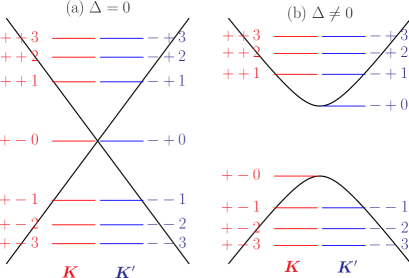
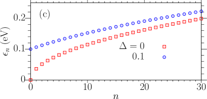
Figure 1: (color online) Illustrations of Landau levels in both valleys for (a) $\Delta=0$ and (b) $\Delta\neq 0$. The black curves are the band structures for zero magnetic field. The Landau levels in $\bm{K}$ ($\bm{K}^{\prime}$) valley are given as red (blue) horizontal lines with level indices $\nu sn$ aside. (c) The energies of Landau levels for (red square) $\Delta=0$ and (blue circle) $\Delta=0.1$ eV.

To summarize, all eigenstates and eigen energies in the $\bm{K}$ valley can be labeled by indices $\{\nu snk\}$ with $\nu=+$, and are given as

$$\Psi_{+snk}(\bm{r}) = \frac{1}{2\sqrt{\pi}}e^{iky}\begin{pmatrix}s\sqrt{1+s\alpha_{n}}\phi_{n-1}(x+l_{c}^{2}k)\\ \sqrt{1-s\alpha_{n}}\phi_{n}(x+l_{c}^{2}k)\end{pmatrix}\,,\quad$$ (10)

$$E_{+snk} = s\epsilon_{n}\,.$$ (11)

Using Eq. (4), we can obtain all eigenstates and eigen energies in the $\bm{K}^{\prime}$ valley as

$$\Psi_{-snk}(\bm{r}) = \sigma_{y}\Psi_{+\bar{s}nk}(\bm{r})\,,$$ (12)

$$E_{-snk} = -E_{+\bar{s}nk}\,,$$ (13)

where the band index $s$ is reversed by hand. They can be organized into a unified form as

$${\begin{array}[]{rcl}E_{\nu snk}&=&s\epsilon_{n}\,,\quad\Psi_{\nu snk}(\bm{r})=\frac{1}{\sqrt{2\pi}}e^{iky}\Phi_{\nu sn}(x+l_{c}^{2}k)\,,\\ \Phi_{\nu sn}(x)&=&\frac{1}{\sqrt{2}}\begin{pmatrix}s\sqrt{1+s\alpha_{n}}\phi_{n-(\nu+1)/2}(x)\\ \sqrt{1-s\alpha_{n}}\phi_{n+(\nu-1)/2}(x)\end{pmatrix}\,,\\ \nu&=&\pm,\quad s=\pm\,,\\ n&\in&\text{integers and }n\geq\frac{1+\nu s}{2}\,.\end{array}}$$

The parameter space of $n$ depends on both $s$ and $\nu$. The eigen energy $E_{\nu snk}$ depends only on the band index $s$ and Landau level index $n$, and each of them has a degeneracy induced by $k$ as ${\cal D}=\frac{1}{2\pi l_{c}^{2}}g_{s}$ with $g_{s}=2$ for spin degeneracy. Figure 1 illustrates the LLs in both valleys for $\Delta=0$ and $\Delta=0.1$ eV. For nonzero $\Delta$, the Landau level $n=0$ in the $\bm{K}$ valley is at the top of the lower band, while the one in the $\bm{K}^{\prime}$ valley is at the bottom of the upper band; As $\Delta$ goes to zero, both of them are at the Dirac points. In this work, we take the Fermi velocity as $v_{F}=10^{6}$ m/s, then the cyclotron energy is $\hbar\omega_{c}\approx 36.3\sqrt{B/1~{}\text{T}}$ meV. In Fig. 1 (c), we show the energies of $\epsilon_{n}$ for $\Delta=0$ and $0.1$ eV.

II.2 Equation of motion and perturbative optical conductivity

When a uniform electric field $\bm{E}(t)$ is applied, the total Hamiltonian is

$$H_{\nu}=H_{\nu;p+e\bm{A}(\bm{r})}^{0}+e\bm{E}(t)\cdot\bm{r}\,.$$ (14)

In the second quantization form, the total Hamiltonian becomes

$$\hat{H}(t)=\sum_{\nu sn}s\epsilon_{n}\int dk\hat{c}_{\nu snk}^{{\dagger}}(t)\hat{c}_{\nu snk}(t)+e\bm{E}(t)\cdot\hat{\bm{r}}(t)\,,$$ (15)

Here $\hat{c}_{\nu snk}(t)$ is the annihilation operator in Heisenberg picture for the state $\Psi_{\nu snk}(\bm{r})$, and it satisfies the anti-commutator $\{\hat{c}_{\nu_{1}s_{1}n_{1}k_{1}},\hat{c}_{\nu_{2}s_{2}n_{2}k_{2}}^{{\dagger}}\}=\delta_{\nu_{1},\nu_{2}}\delta_{s_{1},s_{2}}\delta_{n_{1},n_{2}}\delta(k_{1}-k_{2})$ and $\{\hat{c}_{\nu_{1}s_{1}n_{1}k_{1}},\hat{c}_{\nu_{2}s_{2}n_{2}k_{2}}\}=0$; $\hat{\bm{r}}(t)$ is the position operator in the second quantization form, which is given by

$$\hat{\bm{r}}(t) = \sum_{\nu s_{1}s_{2}\atop n_{1}n_{2}}\bm{\xi}_{\nu;s_{1}n_{1},s_{2}n_{2}}\int dk\hat{c}_{\nu s_{1}n_{1}k}^{{\dagger}}(t)\hat{c}_{\nu s_{2}n_{2}k}(t)$$ (16)

$$+\sum_{\nu sn}\int dk\hat{c}_{\nu snk}^{{\dagger}}(t)\left(-l_{c}^{2}k\hat{\bm{x}}-i\hat{\bm{y}}\frac{\partial}{\partial k}\right)\hat{c}_{\nu snk}(t)\,.\quad\quad$$

The term $\bm{\xi}_{\nu;s_{1}n_{1},s_{2}n_{2}}$ is the Berry connection between states $\Psi_{\nu s_{1}n_{1}}(\bm{r})$ and $\Psi_{\nu s_{2}n_{2}}(\bm{r})$. In the presence of magnetic field, it is convenient to calculate the circularly polarized components $\xi^{\delta}$ defined from a vector $\bm{\xi}=\sum_{\tau=\pm}\xi^{\tau}\hat{\bm{e}}^{\overline{\tau}}$ with $\xi^{\pm}=\frac{1}{\sqrt{2}}(\xi^{x}\pm i\xi^{y})$ and $\hat{\bm{e}}^{\pm}=\frac{1}{\sqrt{2}}(\hat{\bm{x}}\pm i\hat{\bm{y}})$. Here $\tau$ is an index for the circularly polarization direction with taking value from $\pm$, and the notation $\overline{\tau}$ means $\overline{\tau}=-$ ($+$) for $\tau=+$ ($-$). The calculation of Berry connections is listed in Appendix A, which gives

$$\xi_{\nu;s_{1}n_{1},s_{2}n_{2}}^{\tau} = -i\tau w_{s_{1}(n_{2}+\tau),s_{2}n_{2}}^{(\nu\tau)}\delta_{n_{1},n_{2}+\tau}\,,$$ (17)

$$w_{s_{1}n_{1},s_{2}n_{2}}^{(+)} = \frac{l_{c}}{2}\left(s_{1}s_{2}\sqrt{1+s_{1}\alpha_{n_{1}}}\sqrt{1+s_{2}\alpha_{n_{2}}}\sqrt{n_{2}}\right.$$

$$\left.+\sqrt{1-s_{1}\alpha_{n_{1}}}\sqrt{1-s_{2}\alpha_{n_{2}}}\sqrt{n_{1}}\right)\,,$$

$$w_{s_{1}n_{1},s_{2}n_{2}}^{(-)} = w_{s_{2}n_{2},s_{1}n_{1}}^{(+)}\,.$$

Here $(\nu\tau)=(+)$ for $\nu=\tau$ and $(-)$ for $\nu=\overline{\tau}$. The selection rules for $\xi^{\tau}_{\nu;s_{1}n_{1},s_{2}n_{2}}$ between different LLs $n_{1}$ and $n_{2}$ are $n_{1}=n_{2}+\tau$, which is independent of the band index.

The velocity operator is $\hat{\bm{v}}(t)=[\hat{\bm{r}}(t),\hat{H}(t)]/(i\hbar)$, and the current density operator $\hat{\bm{J}}(t)=-e\hat{\bm{v}}(t)$ is

$$\hat{\bm{J}}(t)=-e\sum_{\nu s_{1}s_{2}\atop n_{1}n_{2}}\bm{v}_{\nu;s_{1}n_{1},s_{2}n_{2}}\int dk\hat{c}_{\nu s_{1}n_{1}k}^{{\dagger}}(t)\hat{c}_{\nu s_{2}n_{2}k}(t)\,.$$ (18)

with the matrix elements

$$\bm{v}_{\nu;s_{1}n_{1},s_{2}n_{2}}=i\hbar^{-1}(s_{1}\epsilon_{n_{1}}-s_{2}\epsilon_{n_{2}})\bm{\xi}_{\nu;s_{1}n_{1},s_{2}n_{2}}\,.$$

Because the eigen energies and the velocity matrix elements do not depend on $k$, the dynamics of the current density relies on the dynamics of the effective density matrix operator $\hat{\rho}_{\nu}(t)$, which is defined as

$$\hat{\rho}_{\nu;s_{1}n_{1}s_{2}n_{2}}(t)={\cal D}^{-1}\int dk\hat{c}_{\nu;s_{2}n_{2}k}^{{\dagger}}(t)\hat{c}_{\nu;s_{1}n_{1}k}(t)\,,$$ (19)

with ${\cal D}=1/(\pi l_{c}^{2})$ being the LL degeneracy. The time evolution of $\hat{\rho}_{\nu}(t)$ is determined by the Heisenberg equation

$$i\hbar\frac{\partial\hat{\rho}_{\nu}(t)}{\partial t}=[H_{\nu},\hat{\rho}_{\nu}(t)]+i\hbar\left.\frac{\partial\hat{\rho}_{\nu}(t)}{\partial t}\right|_{scat}\,,$$ (20)

where the last term $\left.\frac{\partial\hat{\rho}_{\nu}(t)}{\partial t}\right|_{scat}$ is the scattering term. By taking the expectation value on both side of above equation with respect to the equilibrium state, we get the matrix elements of $\rho_{\nu;s_{1}n_{1}s_{2}n_{2}}(t)=\langle\hat{\rho}_{\nu;s_{1}n_{1}s_{2}n_{2}}(t)\rangle$ satisfying the equation of motion

$$i\hbar\frac{\partial\rho_{\nu;s_{1}n_{1},s_{2}n_{2}}(t)}{\partial t} = (s_{1}\epsilon_{n_{1}}-s_{2}\epsilon_{n_{2}})\rho_{\nu;s_{1}n_{1},s_{2}n_{2}}(t)$$ (21)

$$+ e\bm{E}(t)\cdot\sum_{sn}\left[\bm{\xi}_{\nu;s_{1}n_{1},sn}\rho_{\nu;sn,s_{2}n_{2}}(t)\right.$$

$$\left.-\rho_{\nu;s_{1}n_{1},sn}(t)\bm{\xi}_{\nu;sn,s_{2}n_{2}}\right]$$

$$- i\Gamma\left[\rho_{\nu;s_{1}n_{1},s_{2}n_{2}}(t)-\rho_{\nu;s_{1}n_{1},s_{2}n_{2}}^{0}\right]\,.\quad\quad$$

Here we describe the scattering by phenomenological relaxation processes with only one relaxation parameter $\Gamma$, $\rho_{\nu;s_{1}n_{1},s_{2}n_{2}}^{0}=\delta_{s_{1},s_{2}}\delta_{n_{1},n_{2}}f_{s_{1}n_{1}}$ is the density matrix element at the equilibrium, $f_{sn}=[1+e^{(s\epsilon_{n}-\mu)/(k_{B}T)}]^{-1}$ is the Fermi-Dirac distribution with a chemical potential $\mu$ and temperature $T$. Note that the $k$ derivative appearing in the Hamiltonian $H(t)$ in Eqs. (15) and (16) does not contribute to the equation of motion, because both the current operator and the density matrix are only related to a term like $\int dk\hat{c}_{k}^{\dagger}\hat{c}_{k}$.

After some algebra listed in the Appendix. B, we get the perturbative linear and third order conductivities. Using the selection rules of $\bm{\xi}$ and $\bm{v}$, the condition for nonzero components of $\sigma^{(1);\tau\alpha}$ is $\tau=\alpha$, and that of $\widetilde{\sigma}^{(3);\tau\alpha\beta\gamma}$ is $\tau=\alpha+\beta+\gamma$. Thus the possible nonzero components of third order conductivity are $\widetilde{\sigma}^{(3);\tau\tau\tau\overline{\tau}}$, $\widetilde{\sigma}^{(3);\tau\tau\overline{\tau}\tau}$, and $\widetilde{\sigma}^{(3);\tau\overline{\tau}\tau\tau}$. The linear conductivity is expressed as

$$\sigma^{(1);\tau\tau}(\omega) = -\frac{ie^{2}}{\hbar}{\cal D}\sum_{\nu s_{1}s_{2}}\sum_{n}\frac{(s_{2}\epsilon_{n+\tau}-s_{1}\epsilon_{n})[w_{s_{2}(n+\tau),s_{1}n}^{(\nu\tau)}]^{2}(f_{s_{2}(n+\tau)}-f_{s_{1}n})}{\hbar\omega+i\Gamma-(s_{1}\epsilon_{n}-s_{2}\epsilon_{n+\tau})}\,,$$ (22)

Although the inversion symmetry is broken for a nonzero mass term $\Delta$, the second order response of optical current is still zero in our approach because the linear dispersion approximation in $H_{\nu;\bm{p}}^{0}$ includes an additional inversion symmetry; the nonzero second order response can be obtained beyond the linear dispersion approximation. The third order conductivities are

$$\sigma^{(3);\tau\alpha\beta\gamma}(\omega_{1},\omega_{2},\omega_{3}) = \frac{1}{6}\left[\widetilde{\sigma}^{(3);\tau\alpha\beta\gamma}(w,\hbar(\omega_{2}+\omega_{3})+i\Gamma,\hbar\omega_{3}+i\Gamma)+\widetilde{\sigma}^{(3);\tau\alpha\gamma\beta}(w,\hbar(\omega_{2}+\omega_{3})+i\Gamma,\hbar\omega_{2}+i\Gamma)\right.$$ (23)

$$+\widetilde{\sigma}^{(3);\tau\beta\alpha\gamma}(w,\hbar(\omega_{1}+\omega_{3})+i\Gamma,\hbar\omega_{3}+i\Gamma)+\widetilde{\sigma}^{(3);\tau\beta\gamma\alpha}(w,\hbar(\omega_{1}+\omega_{3})+i\Gamma,\hbar\omega_{1}+i\Gamma)$$

$$\left.+\widetilde{\sigma}^{(3);\tau\gamma\alpha\beta}(w,\hbar(\omega_{1}+\omega_{2})+i\Gamma,\hbar\omega_{2}+i\Gamma)+\widetilde{\sigma}^{(3);\tau\gamma\beta\alpha}(w,\hbar(\omega_{1}+\omega_{2})+i\Gamma,\hbar\omega_{1}+i\Gamma)\right]\,,$$

with $w=\hbar(\omega_{1}+\omega_{2}+\omega_{3})+i\Gamma$ and

$$\widetilde{\sigma}^{(3);\tau\alpha\beta\gamma}(w,w_{0},w_{3})$$ (24)

$$= -\frac{ie^{4}}{\hbar}{\cal D}\sum_{\nu s_{1}s_{2}\atop s_{3}s_{4}}\sum_{n}\frac{(s_{2}\epsilon_{n}-s_{1}\epsilon_{n-\tau})w_{s_{2}n,s_{1}(n-\tau)}^{(\nu\tau)}}{w-(s_{1}\epsilon_{n-\tau}-s_{2}\epsilon_{n})}\frac{w_{s_{1}(n-\tau),s_{3}(n-\gamma-\beta)}^{(\nu\overline{\alpha})}}{w_{0}-(s_{3}\epsilon_{n-\gamma-\beta}-s_{2}\epsilon_{n})}$$

$$\times\left[\frac{w_{s_{3}(n-\gamma-\beta),s_{4}(n-\gamma)}^{(\nu\overline{\beta})}w_{s_{4}(n-\gamma),s_{2}n}^{(\nu\overline{\gamma})}(f_{s_{2}n}-f_{s_{4}(n-\gamma)})}{w_{3}-(s_{4}\epsilon_{n-\gamma}-s_{2}\epsilon_{n})}\right.$$

$$\quad\quad\left.-\frac{w_{s_{3}(n-\beta-\gamma),s_{4}(n-\beta)}^{(\nu\overline{\gamma})}w_{s_{4}(n-\beta),s_{2}n}^{(\nu\overline{\beta})}(f_{s_{4}(n-\beta)}-f_{s_{3}(n-\beta-\gamma)})}{w_{3}-(s_{3}\epsilon_{n-\beta-\gamma}-s_{4}\epsilon_{n-\beta})}\right]$$

$$+ \frac{ie^{4}}{\hbar}{\cal D}\sum_{\nu s_{1}s_{2}\atop s_{3}s_{4}}\sum_{n}\frac{(s_{2}\epsilon_{n}-s_{1}\epsilon_{n-\tau})w_{s_{2}n,s_{1}(n-\tau)}^{(\nu\tau)}}{w-(s_{1}\epsilon_{n-\tau}-s_{2}\epsilon_{n})}\frac{w_{s_{4}(n-\alpha),s_{2}n}^{(\nu\overline{\alpha})}}{w_{0}-(s_{1}\epsilon_{n-\tau}-s_{4}\epsilon_{n-\alpha})}$$

$$\times\left[\frac{w_{s_{1}(n-\tau),s_{3}(n-\gamma-\alpha)}^{(\nu\overline{\beta})}w_{s_{3}(n-\gamma-\alpha),s_{4}(n-\alpha)}^{(\nu\overline{\gamma})}(f_{s_{4}(n-\alpha)}-f_{s_{3}(n-\gamma-\alpha)})}{w_{3}-(s_{3}\epsilon_{n-\gamma-\alpha}-s_{4}\epsilon_{n-\alpha})}\right.$$

$$\quad\quad\left.-\frac{w_{s_{1}(n-\tau),s_{3}(n-\alpha-\beta)}^{(\nu\overline{\gamma})}w_{s_{3}(n-\alpha-\beta),s_{4}(n-\alpha)}^{(\nu\overline{\beta})}(f_{s_{3}(n-\alpha-\beta)}-f_{s_{1}(n-\tau)})}{w_{3}-(s_{1}\epsilon_{n-\tau}-s_{3}\epsilon_{n-\alpha-\beta})}\right]\,.$$

It is constructive to give the tensor components in Cartesian coordinates. The independent Cartesian components of the linear conductivity are $\sigma^{(1);xx}(\omega)=\sigma^{(1);yy}(\omega)$ and $\sigma^{(1);yx}(\omega)=-\sigma^{(1);xy}$, which can be expressed as

$$\sigma^{(1);xx}(\omega) = \dfrac{1}{2}\sum_{\tau}\sigma^{(1);\tau\tau}(\omega)\,,$$

$$\sigma^{(1);yx}(\omega) = -\dfrac{i}{2}\sum_{\tau}\tau\sigma^{(1);\tau\tau}(\omega)\,.$$ (25)

The independent Cartesian components of the third order conductivity are $\sigma^{(3);dxyy}$, $\sigma^{(3);dyxy}$, and $\sigma^{(3);dyyx}$ with $d=x,y$. The other components can be obtained by $\sigma^{(3);dxxx}=\sigma^{(3);dxyy}+\sigma^{(3);dyxy}+\sigma^{(3);dyyx}$ and by the symmetry $\{x\leftrightarrow y\}$. In this work, we are interested in $\sigma^{(3);dxxx}$, which can be expressed as

$$\sigma^{(3);xxxx} = \frac{1}{4}\sum_{\tau}\left(\sigma^{(3);\tau\tau\tau\overline{\tau}}+\sigma^{(3);\tau\tau\overline{\tau}\tau}+\sigma^{(3);\tau\overline{\tau}\tau\tau}\right)\,,$$

$${\sigma}^{(3);yxxx} = -\frac{i}{4}\sum_{\tau}\tau\left(\sigma^{(3);\tau\tau\tau\overline{\tau}}+\sigma^{(3);\tau\tau\overline{\tau}\tau}+\sigma^{(3);\tau\overline{\tau}\tau\tau}\right)\,.\quad\quad$$ (26)

Obviously, the independent components $\sigma^{(1);xx}$, $\sigma^{(3);xxyy}$, $\sigma^{(3);xyxy}$, and $\sigma^{(3);xyyx}$ are nonzero regardless of the value of the magnetic field, while those of $\sigma^{(1);xy}$, $\sigma^{(3);xyxx}$, $\sigma^{(3);xxyx}$, and $\sigma^{(3);xxxy}$ are not zero only at nonzero magnetic field.

II.3 Resonance and electron-hole symmetry

Here we discuss two general properties of the conductivity. The first is related to the resonant transitions. At a finite magnetic field, all electronic levels are discrete, and both the linear conductivity and the nonlinear conductivity posses many resonant peaks. As an example, the transition diagrams for the unsymmetrized third order conductivity $\widetilde{\sigma}^{(3);\tau\alpha\beta\gamma}(w,w_{0},w_{3})$ in Eq. (24) are shown in Fig. 2.

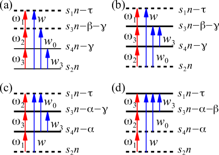
Figure 2: (color online) Optical transitions for $\widetilde{\sigma}_{\nu}^{(3);\tau{\alpha}{\beta}{\gamma}}(w,w_{0},w_{3})$ with $w_{3}=\hbar\omega_{3}+i\Gamma$, $w_{0}=\hbar(\omega_{2}+\omega_{3})+i\Gamma$, and $w=\hbar(\omega_{1}+\omega_{2}+\omega_{3})+i\Gamma$. The subfigures (a), (b), (c), and (d) correspond to the four terms in Eq. (24), respectively. The horizontal lines indicate the LLs, where the indices “$sn$” are labeled at the right; the dashed lines mean the virtual states, while the two solid lines stand for a pair of occupied and unoccupied states; the red arrows indicate the optical transitions with the involved photon frequency $\omega_{i}$ labeled aside; the blue arrows stand for the energies involved in the denominators.

Because the indices $\tau\alpha\beta\gamma$ can only take the values $\pm 1$, each transition involves three photon energies, four bands indices, and at most three and at least two Landau indices. Three arrows associated with $w$, $w_{0}$, and $w_{3}$ correspond to the three energy factors, in a form

$${\cal E}_{s_{1}s_{2}}(w,n,m)=w-(s_{1}\epsilon_{n+m}-s_{2}\epsilon_{n})\,,$$ (27)

appearing in the denominator of the expression in Eq. (24). When ${\cal E}_{s_{1}s_{2}}(w,n,m)=0$, the optical transitions are in resonance, and third order nonlinear conductivity may diverge. The condition ${\cal E}_{ss}(w,n,m)=0$ determines the resonant intraband transition, while the condition ${\cal E}_{s\bar{s}}(w,n,m)=0$ determines the resonant interband transition. The expression of $\widetilde{\sigma}^{(3);\tau\alpha\beta\gamma}(w,w_{0},w_{3})$ includes four full denominators,

$${\cal E}_{s_{1}s_{2}}(w,n,\overline{\tau}){\cal E}_{s_{3}s_{2}}(w_{0},n,\overline{\beta}+\overline{\gamma}){\cal E}_{s_{4}s_{2}}(w_{3},n,\overline{\gamma})\,,$$

$${\cal E}_{s_{1}s_{2}}(w,n,\overline{\tau}){\cal E}_{s_{3}s_{2}}(w_{0},n,\overline{\beta}+\overline{\gamma}){\cal E}_{s_{3}s_{4}}(w_{3},n-\beta,\overline{\gamma})\,,$$

$${\cal E}_{s_{1}s_{2}}(w,n,\overline{\tau}){\cal E}_{s_{1}s_{4}}(w_{0},n-\alpha,\overline{\beta}+\overline{\gamma}){\cal E}_{s_{3}s_{4}}(w_{3},n-\alpha,\overline{\gamma})\,,$$

$${\cal E}_{s_{1}s_{2}}(w,n,\overline{\tau}){\cal E}_{s_{1}s_{4}}(w_{0},n-\alpha,\overline{\beta}+\overline{\gamma}){\cal E}_{s_{2}s_{3}}(w_{3},n-\alpha-\beta,\overline{\gamma})\,.$$

Each of them is composed of three energy factors, depending on field frequency $\omega_{i}$, magnetic field $B$, gap parameter $\Delta$, the Landau indices, and the polarization of the incident light. By varying these parameters, one or more ${\cal E}$ can be zero and lead to a resonance. Usually each energy factor contributes one Lorentz-type divergence as $(\delta E+i\Gamma)^{-1}$. Two energy factors in the denominator may be the same, which could lead to a higher order divergence as $(\delta E+i\Gamma)^{-2}$. Also, it can not be excluded that for some special parameters ($n$, $s_{i}$, $\mu$, $\Delta$, $B$, and $\omega_{i}$) all three energy factors simultaneously satisfy the resonant conditions, and lead to a higher order divergence Yao and Belyanin (2012). We will use this analysis for understanding the peaks in the spectra of the conductivities.

The second is a chemical potential dependence of the conductivity that is related to the electron-hole symmetry. For convenience, we explicitly show the chemical potential dependence as $\sigma^{(1);\tau\alpha}_{\nu}(\omega,\mu)$, $\sigma^{(3);\tau\alpha\beta\gamma}_{\nu}(\omega_{1},\omega_{2},\omega_{3},\mu)$, and $f_{\nu sn}(\mu)$, where the subscript $\nu$ indicates the contribution from each valley. We use the relations in Eqs. (47) and (48), as well as

$$f_{\nu sn}(\mu)=1-f_{\overline{\nu}\bar{s}n}(-\mu)\,,$$ (28)

where the energy relations between two valleys $E_{\nu sn}=-E_{\overline{\nu}\overline{s}n}$ is used. Checking the expressions in Eqs. (22) and (24) we can directly obtain

$$\sigma^{(1);\delta\alpha}_{\tau}(\omega,\mu) = \sigma_{\overline{\tau}}^{(1);\overline{\delta}\overline{\alpha}}(\omega,-\mu)\,,$$ (29)

$$\sigma^{(3);\delta\alpha\beta\gamma}_{\tau}(\omega_{1},\omega_{2},\omega_{3},\mu) = \sigma_{\overline{\tau}}^{(1);\overline{\delta}\overline{\alpha}\overline{\beta}\overline{\gamma}}(\omega_{1},\omega_{2},\omega_{3},-\mu)\,.\quad$$ (30)

Using these relations and from Eqs. (25) and (26), the independent components $\sigma^{(1);xx}$, $\sigma^{(3);xxyy}$, $\sigma^{(3);xyxy}$, and $\sigma^{(3);xyyx}$ are even functions of the chemical potential, while the other independent components $\sigma^{(1);xy}$, $\sigma^{(3);xyxx}$, $\sigma^{(3);xxyx}$, and $\sigma^{(3);xxxy}$ are odd functions of the chemical potential. Therefore, for intrinsic graphene $\mu=0$ or GG, all transverse optical conductivities are zero, e.g., $\sigma^{(1);xy}(\mu=0)=0$, for all temperature.

In the following sections we discuss the linear conductivity and nonlinear conductivities associated with nonlinear phenomena including THG, NL, and FWM. For an incident light $\bm{E}(t)=\bm{E}_{\omega}e^{-i\omega t}+c.c.$, the generated nonlinear current for THG is

$$\bm{J}_{\text{THG}}(t) = e^{-i3\omega t}\bm{E}_{\omega}\cdot\bm{E}_{\omega}\left[\sigma^{(3);xxxx}(\omega,\omega,\omega)\bm{E}_{\omega}+\sigma^{(3);yxxx}(\omega,\omega,\omega)\hat{\bm{z}}\times\bm{E}_{\omega}\right]+c.c.$$ (31)

$$= e^{-i3\omega t}E_{\omega}^{+}E_{\omega}^{-}\left[3\sigma^{(3);+++-}(\omega,\omega,\omega)E_{\omega}^{+}\hat{\bm{e}}^{-}+3\sigma^{(3);---+}(\omega,\omega,\omega)E_{\omega}^{-}\hat{\bm{e}}^{+}\right]+c.c.\,;$$

for incident light $\bm{E}(t)=\bm{E}_{\omega_{p}}e^{-i\omega_{p}t}+\bm{E}_{-\omega_{s}}e^{i\omega_{s}t}+c.c.$, the nonlinear current for FWM is

$$\bm{J}_{\text{FWM}}(t) = e^{-(2\omega_{p}-\omega_{s})t}\left\{\left[2\sigma^{(3);xxyy}(\omega_{p},\omega_{p},-\omega_{s})\bm{E}_{\omega_{p}}+2\sigma^{(3);xyxx}(\omega_{p},\omega_{p},-\omega_{s})\bm{E}_{\omega_{p}}\times\hat{\bm{z}}\right]\bm{E}_{\omega_{p}}\cdot\bm{E}_{-\omega_{s}}\right.$$ (32)

$$\left.+\left[\sigma^{(3);xyyx}(\omega_{p},\omega_{p},-\omega_{s})\bm{E}_{-\omega_{s}}+\sigma^{(3);xxxy}(\omega_{p},\omega_{p},-\omega_{s})\bm{E}_{-\omega_{s}}\times\hat{\bm{z}}\right]\bm{E}_{\omega_{p}}\cdot\bm{E}_{\omega_{p}}\right\}+c.c.$$

$$= e^{-(2\omega_{p}-\omega_{s})t}\sum_{\tau}\hat{\bm{e}}^{\overline{\tau}}\left[\sigma^{(3);\tau\tau\tau\overline{\tau}}(\omega_{p},\omega_{p},-\omega_{s})E_{\omega_{p}}^{\tau}+2\sigma^{(3);\overline{\tau}{\tau}\overline{\tau}{\tau}}(\omega_{p},\omega_{p},-\omega_{s})E_{\omega_{p}}^{\overline{\tau}}\right]E_{\omega_{p}}^{\tau}E_{-\omega_{s}}^{\overline{\tau}}+c.c.\,.$$

By setting $\omega_{s}=\omega_{p}=\omega$, we can get the nonlinear current for the NL process. Due to the symmetry of graphene, there is no THG for single circularly polarized incident light. We focus on the longitudinal current for incident light along the $x$ direction, and note

$$\begin{array}[]{rcl}\sigma^{xxxx}_{\text{THG}}(\omega)&=&\sigma^{(3);xxxx}(\omega,\omega,\omega)\,,\\ \sigma^{xxxx}_{\text{nl}}(\omega)&=&\sigma^{(3);xxxx}(\omega,\omega,-\omega)\,,\\ \sigma_{\text{FWM}}^{xxxx}(\omega_{p},\omega_{s})&=&\sigma^{(3);xxxx}(\omega_{p},\omega_{p},\omega_{s})\,.\end{array}$$ (33)

The transverse conductivities are about two orders of magnitude smaller than the longitudinal ones for most parameters, and are ignored in this work.

III Optical conductivities at weak magnetic field

We first consider the conductivities in a weak magnetic field, where $\hbar\omega_{c}$ is much smaller than the relaxation parameters, the thermal energy, and the involved photon energies. The optical transitions between Landau levels can not be resolved, and it is natural to treat the discrete LLs as continuous levels. As $B\to 0$, the sum over the Landau level index $n$ in Eqs. (22) and (24) can be transformed into an integration over $x$ by the substitution $\epsilon_{n}\to x$, $\epsilon_{n+\tau}\to x+\tau(\hbar\omega_{c})^{2}F_{0}(x)$, and $w^{(\nu\tau)}_{s_{1}n+\tau_{1};s_{2}n+\tau_{2}}\to F(x)+\tau_{1}(\hbar\omega_{c})^{2}F_{1}(x)+\tau_{2}(\hbar\omega_{c})^{2}F_{2}(x)$, where the explicit expression of $F_{i}(x)$ are not important for our next discussion. For linear conductivity $\sigma^{(1);\tau\tau}(\omega)$, the contribution from the weak magnetic field depends on $\tau(\hbar\omega_{c})^{2}\propto\tau B$, thus we get

$$\sigma^{(1);\tau\tau}(\omega)=S^{(1)}_{0}(\omega)-iS^{(1)}_{1}(\omega)B\tau+S^{(1)}_{2}(\omega)B^{2}+\cdots\,.$$ (34)

At weak magnetic field, the leading term of the linear conductivity is

$$\sigma^{(1);xx}(\omega) \approx S^{(1)}_{0}(\omega)\,,$$ (35)

$$\sigma^{(1);xy}(\omega) \approx S^{(1)}_{1}(\omega)B\,.$$ (36)

Similarly, the third order conductivities can be approximated as

$$\sigma^{(3);xxxx}(\omega_{1},\omega_{2},\omega_{3}) \approx S^{(3)}_{0}(\omega_{1},\omega_{2},\omega_{3})\,,$$ (37)

$$\sigma^{(3);yxxx}(\omega_{1},\omega_{2},\omega_{3}) \approx S^{(3)}_{1}(\omega_{1},\omega_{2},\omega_{3})B\,.$$ (38)

The study of this limit has two aims. One is a validity check by comparing our conductivities of doped graphene at very weak magnetic field with those at zero magnetic field, which are already presented in the literature. The other is to approach the third order conductivities for gapped graphene at zero magnetic field.

III.1 Comparison with literature

In the absence of the magnetic field, the optical conductivities of DG have been systematically studied both analytically Cheng et al. (2014, 2015a); Mikhailov (2016) and numerically Cheng et al. (2015b). In the linear dispersion approximation and describing the relaxation in a phenomenological way, analytic expressions are found for linear Hanson (2008), second order Wang et al. (2016); Cheng et al. (2017); Rostami et al. (2017), and third order conductivities Cheng et al. (2015a); Mikhailov (2016). For GG, the linear conductivity has analytic expression for transitions around the Dirac points, and some of the nonlinear conductivities have been numerically extracted Cheng et al. (2015b). All those conductivities are based on a plane wave basis. In this work, these conductivities are considered from a different approach, based on the LLs, and it is interesting to compare them.

Our calculations are done for parameters $B=0.05$ T. Here the treatment of $0.05$ T as weak field can be clearly seen in section IV. Other parameters are $\Gamma=10$ meV, the temperature $T=10$ K, and the Landau index $n$ is taken as $n<N_{c}$ with a cutoff $N_{c}$. For high photon energy, large $N_{c}$ is required for the convergence of the conductivities. Because the photon energy can be as high as around 1 eV, we choose $N_{c}=2\times 10^{6}$ (corresponding to an energy cutoff $\sim 11$ eV) for the calculation of linear conductivity, and $N_{c}=10^{6}$ (the energy cutoff is $\sim 8$ eV) for the nonlinear conductivities. The spectra of the conductivities of DG are plotted in Fig. 3 as thin curves for $\sigma^{(1);xx}$, $\sigma^{xxxx}_{\text{THG}}$, $\sigma^{xxxx}_{\text{nl}}$, and $\sigma^{xxxx}_{\text{FWM}}$; and the linear conductivity of GG $\sigma^{(1);xx}$ is shown in Fig. 3 (a) as thick curves.

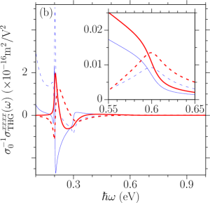
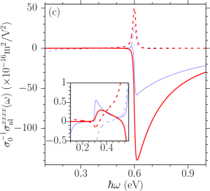
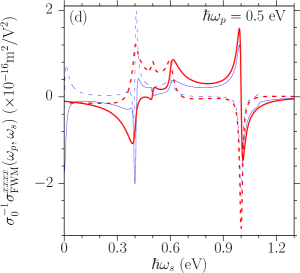
Figure 3: (color online) Spectra of optical conductivities for DG at $\mu=-0.3$ eV (blue thin curves) and GG at $\Delta=0.3$ eV (red thick curves). (a) $\sigma^{(1);xx}(\omega)$, (b) $\sigma^{xxxx}_{\text{THG}}(\omega)$, (c) $\sigma^{xxxx}_{\text{nl}}(\omega)$, (d) $\sigma^{xxxx}_{\text{FWM}}(\omega_{p},\omega)$. The solid (dashed) curves are for the real (imaginary) parts, respectively. The insets in (b) and (c) show the details in given range of the photon energies. Other parameters are $B=0.05$ T, $T=10$ K, and $\Gamma=10$ meV.

The obtained curves overlap with those from analytic expressions Cheng et al. (2015a, b), confirming the equivalence between the LL basis and the plane wave basis.

The comparison can be further extended to the linear conductivity $\sigma^{(1);xy}(\omega)$ or $S_{1}^{(1)}(\omega)$, which is related to the second order conductivities induced by magnetic dipole interactions. In DG, the second order current Cheng et al. (2017) can be expressed as

$$\bm{J}^{(2)}(\bm{r},t) = 2\int\frac{d\bm{q}_{1}d\bm{q}d\omega_{1}d\omega}{(2\pi)^{6}}e^{-i(\omega_{1}+\omega)t+i(\bm{q}_{1}+\bm{q})\cdot\bm{r}}$$ (39)

$$\times\Big{\{}S_{M}^{xxyy}(\omega_{1},\omega)[\bm{q}_{1}\times\bm{E}(\bm{q}_{1}\omega_{1})]\times\bm{E}(\bm{q}\omega)$$

$$+S_{Q}^{xyxy}(\omega_{1},\omega)\bm{q}_{1}\cdot\bm{E}(\bm{q}_{1}\omega_{1})\bm{E}(\bm{q}\omega)$$

$$+S_{Q}^{xxyy}(\omega_{1},\omega)[\bm{E}(\bm{q}_{1}\omega_{1})\bm{q}_{1}\cdot\bm{E}(\bm{q}\omega)$$

$$+\bm{q}_{1}\bm{E}(\bm{q}_{1}\omega_{1})\cdot\bm{E}(\bm{q}\omega)]\Big{\}}\,.$$

In the linear dispersion approximation, the coefficients $S^{xxyy}_{M}$, $S^{xyxy}_{Q}$, and $S^{xxyy}_{Q}$ have analytic expressions Cheng et al. (2017), where the term involving $S_{M}^{xxyy}$ gives the contribution induced by the magnetic dipole interaction. Using the relation $\bm{B}(\bm{q}_{1}\omega_{1})=\frac{1}{\omega_{1}}\bm{q}_{1}\times\bm{E}(\bm{q}_{1}\omega_{1})$ and taking the limit $\bm{q}_{1},\omega_{1},\bm{q}\to 0$, we can recover the uniform magnetic field, and obtain

$$S^{(1)}_{1}(\omega) = \lim\limits_{\omega_{1}\to 0}\left[2\omega_{1}S_{M}^{xxyy}(\omega_{1},\omega)-2\omega_{1}S_{M}^{xxyy}(-\omega_{1},\omega)\right]$$ (40)

$$= -\text{sgn}(\mu)\sigma_{0}\frac{2e(\hbar v_{F})^{2}}{\pi\hbar}\frac{1}{(\hbar\omega)^{2}}\left(\frac{8\mu^{2}}{w^{2}-4\mu^{2}}\right.$$

$$\left.+\frac{8\mu^{2}}{\Gamma^{2}+4\mu^{2}}\frac{2w-i\Gamma}{w}\right)\,,$$

with $w=\hbar\omega+i\Gamma$ and the universal conductivity $\sigma_{0}=e^{2}/(4\hbar)$. In the absence of the relaxation, $S_{1}^{(1)}(\omega)$ agrees with the calculated $\sigma^{(1);xy}(\omega)$ very well.

These two approaches show excellent agreement, which provides a good validity check of the approach based on the LLs. Furthermore, the nonlinear conductivities of GG in the absence of the magnetic field, which has not been systematically studied before, can be obtained from Eqs. (22) and (24) at very weak magnetic field $B=0.05$ T.

III.2 Third order conductivities of GG

We calculate the optical conductivity of GG for a gap parameter $\Delta=0.3$ eV and a chemical potential $\mu=0$ eV. Other parameters are $B=0.05$ T, $T=10$ K, and $\Gamma=10$ meV, which are the same as those in previous section. The largest energy difference between adjacent Landau levels is $\epsilon_{1}-\epsilon_{0}\sim 0.1$ meV, which is much smaller than the relaxation parameter $\Gamma$, and the discreteness of the levels can be smeared out by the relaxation parameters. In Fig. 3 we show the calculated conductivities of GG in thick curves. Because the system has a nonzero gap $2\Delta=0.6$ eV and it is not doped, both the linear and nonlinear conductivities are insensitive to temperature. In DG, the chemical potential $\mu$ can be used to tune the optical nonlinearity because it acts like a chemical potential induced gap for interband transitions, and leads to resonant responses. Analogically, the real gap $2\Delta$ in GG is expected to play similar role. Here we discuss their similarities and differences.

For simplicity we first look at the linear conductivity. As we discussed in the previous section, our calculations are in agreement with the analytic expressions Cheng et al. (2015b). Our numerical results are shown in Fig. 3(a). With photon energy increasing from 0.1 eV to 1 eV, the real part of the linear conductivity is zero for about $\hbar\omega<2\Delta$, quickly turns on for $\hbar\omega\sim 2\Delta$, and then decreases with photon energy to $\sigma_{0}=e^{2}/(4\hbar)$. The imaginary part is negative for all photon energies, which shows the dielectric properties of a gapped graphene. Its magnitude increases from zero at $\hbar\omega=0$ (from the analytic expression) to a maximum value around $\hbar\omega\sim 2\Delta$, and then decreases. Compared to the conductivity of DG at $\mu=\Delta$, there are two main differences: (i) The Drude conductivity disappears because the thermal excited carriers can be ignored, and thus the gapped graphene acts as a dielectric material. (ii) The value of the real part at the photon energy around the gap is larger than that of DG, which can be attributed to the larger values of the dipole matrix elements shown in Fig. 8; similarly, the peak value of its imaginary part is also larger than that of DG.

Now we turn to the nonlinear conductivities of GG. The spectra of $\sigma^{xxxx}_{\text{THG}}(\omega)$ for THG, $\sigma^{xxxx}_{\text{nl}}(\omega)$ for NL, and $\sigma^{xxxx}_{\text{FWM}}(\omega_{p},\omega_{s})$ for FWM are plotted in Fig. 3 (b), (c), and (d), respectively. All spectra show complicated dependence on the photon energy, and they include many resonant peaks. For $\sigma^{xxxx}_{\text{THG}}(\omega)$ in Fig. 3 (b), its value is almost zero at $\hbar\omega=0.1$ eV. With increasing the photon energy, its magnitude increases and reaches a resonant value around $2\times 10^{-16}\times\sigma_{0}$ m²/V² at photon energy $\hbar\omega=0.2$ eV. Then its magnitude generally decreases with the photon energy, and shows two more resonant features around $\hbar\omega=0.3$ eV and $0.6$ eV, but with smaller peak values. The fine structures of $\sigma^{xxxx}_{\text{THG}}$ are located at $\hbar\omega\sim 0.2$ eV, $0.3$ eV, and $0.6$ eV. For $\sigma^{xxxx}_{\text{nl}}(\omega)$ in Fig. 3 (c), we first look at the real part $\text{Re}[\sigma^{xxxx}_{\text{nl}}(\omega)]$. Its value remains close to zero for photon energies $\hbar\omega<0.3$ eV, increases quickly to reach a peak value $\sim 0.3\times 10^{-16}\times\sigma_{0}$ m²/V² around $\hbar\omega\sim 0.35$ eV, and then decreases to cross zero around $\hbar\omega\sim 0.53$ eV. For greater photon energies, the real part reaches a valley with a negative value $\sim-140\times 10^{-16}\times\sigma_{0}$ m²/V² at $\hbar\omega\sim 0.61$ eV. At higher photon energies, its value increases monotonically towards zero. The imaginary part $\text{Im}[\sigma^{xxxx}_{\text{nl}}(\omega)]$ decreases from $\sim 0.07\times 10^{-16}\times\sigma_{0}$ m²/V² at $\hbar\omega=0.1$ eV to a value $\sim-0.15\times 10^{-16}\times\sigma_{0}$ m²/V² at $\hbar\omega\sim 0.31$ eV, then it increases to a peak with value $\sim 50\times 10^{-16}\times\sigma_{0}$ m²/V² at $\hbar\omega\sim 0.6$ eV, and finally decreases to small values for higher photon energy. The fine structures are located at $\hbar\omega\sim 0.3$ eV and $0.6$ eV. The spectrum of $\sigma^{xxxx}_{\text{FWM}}(\omega_{p},\omega_{s})$ in Fig. 3 (d) shows even more complicated structures, which are separated by photon energies at $\hbar\omega\sim 0.4$ eV, $0.5$ eV, $0.6$ eV, and $1.0$ eV. The values are also at the order of magnitude of $10^{-16}\times\sigma_{0}$ m²/V².

All these features can also be found in the spectra of conductivities of DG (thin curves in the same figure), and are all induced by the resonant interband transitions. Some of them are related to the energy of the gap ($E_{g}=2\Delta$ for GG or $E_{g}=2|\mu|$ for DG), with matching the involved photon energies or their sum with the gap energy. For THG, the conditions are $E_{g}=\hbar\omega$, $2\hbar\omega$, or $3\hbar\omega$; for NL, they are $E_{g}=\hbar\omega$ or $E_{g}=2\hbar\omega$; and for FWM, they are $E_{g}=2\hbar\omega_{p}-\hbar\omega_{s}$ and $\hbar\omega_{s}$. The other two resonant features in FWM occur at the conditions $\hbar\omega_{s}=\hbar\omega_{p}$ and $\hbar\omega_{s}=2\hbar\omega_{p}$. They arise from the optically excited free carriers. In fact, for $\hbar\omega_{s}=\hbar\omega_{p}$, FWM reduces to NL $\sigma^{xxxx}_{\text{nl}}(\omega_{p})=\sigma^{xxxx}_{\text{FWM}}(\omega_{p},\omega_{p})$. In our calculation, the NL is finite and the corresponding structure in the spectra of FWM does not change too much. The other condition $\hbar\omega_{s}=2\hbar\omega_{p}$ corresponds to two-color coherent current injection, which show a Lorentz-type divergence as $(\hbar\delta\omega+i\Gamma)^{-1}$ for small $\hbar\delta\omega=2\hbar\omega_{p}-\hbar\omega_{s}$. We conclude that these fine structures of the spectra in GG also come from the interband resonant transitions, and the chemical potential in DG and the gap parameter in GG do have similar role for the interband transition. The values of the resonant peaks of DG and GG are of the same order of magnitude, but differ by a factor of two or three. Some of them are larger and sharper for DG than those for GG, such as the resonance at $0.2$ eV for THG, that at $0.3$ eV for NL, and that at $0.4$ eV for FWM. In general, other peaks for DG are lower than those for GG, similar to that of the linear conductivity.

The differences between the conductivities of DG and GG are also obvious, especially around the zero photon energies. All conductivities of DG show a Drude-like contribution, which tends to diverge for zero photon energy (or large finite value with the inclusion of relaxation). In the relaxation free case, the third order nonlinear conductivities of DG behave as $\sigma^{xxxx}\propto\omega^{-4}$. However, all conductivities of GG at low photon energies give small values; this is consistent with a general conclusion for cold and clean dielectric materials. Aversa and Sipe Aversa and Sipe (1995) have theoretically shown that for a cold and clean dielectric material, the value of $\chi^{(3)}$ should be zero as all frequencies go to zero, which means $\sigma^{xxxx}_{\text{THG}}(0)=0$ and $\sigma^{xxxx}_{\text{nl}}(0)=0$.

This distinction can be further understood from the peaks in Fig. 4, where the absolute values of conductivities are plotted with varying $\mu$ for DG or $\Delta$ for GG. The

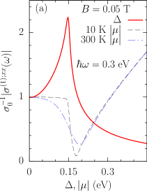
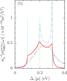
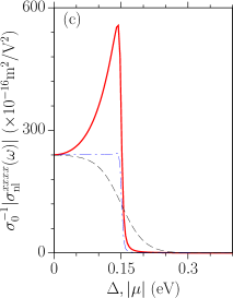
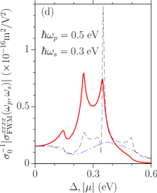
Figure 4: (color online) The $|\mu|$ ($\Delta$) dependence of optical conductivities of DG (GG). (a) $|\sigma^{(1);xx}(\omega)|$, (b) $|\sigma^{xxxx}_{\text{THG}}(\omega)|$, (c) $|\sigma^{xxxx}_{\text{nl}}(\omega)|$, (d) $|\sigma^{xxxx}_{\text{FWM}}(\omega_{p},\omega_{s})|$. The photon energies are chosen as $\hbar\omega=\hbar\omega_{s}=0.3$ eV, $\hbar\omega_{p}=0.5$ eV. Other parameters are $B=0.05$ T and $\Gamma=10$ meV.

photon energies are chosen as $\hbar\omega=\hbar\omega_{s}=0.3$ eV and $\hbar\omega_{p}=0.5$ eV, the magnetic field is $B=0.05$ T, and the temperature is $T=10$ K as well as $300$ K. Note that for a finite gap $\Delta\gg k_{B}T$, all conductivities of GG are insensitive to the temperature; however, temperature remarkably affects those of DG, even smearing out some peaks, as shown in Fig. 4 for $T=10$ K and $300$ K.

IV Magnetic field dependence of optical conductivities

In this section we examine how the magnetic field affects optical conductivities $\sigma^{(1);xx}(\omega)$, $\sigma^{xxxx}_{\text{nl}}(\omega)$, $\sigma^{xxxx}_{\text{THG}}(\omega)$, and $\sigma^{xxxx}_{\text{FWM}}(\omega_{p},\omega_{s})$. The calculations are performed for different gap parameters for GG and chemical potential for DG at a relaxation parameter $\Gamma=10$ meV, temperature $T=10$ K, and fixed photon energies $\hbar\omega=\hbar\omega_{s}=0.3$ eV and $\hbar\omega_{p}=0.5$ eV. The cutoff of the Landau index $N_{c}$ is chosen to satisfy the cutoff energy to be at the order of 10 eV.

IV.1 Results of GG

In Fig. 5, we present the absolute values of conductivities $\sigma^{(1);xx}(\omega)$, $\sigma^{xxxx}_{\text{nl}}(\omega)$, $\sigma^{xxxx}_{\text{THG}}(\omega)$, and $\sigma^{xxxx}_{\text{FWM}}(\omega_{p},\omega_{s})$ of a gapped graphene with varying the magnetic field $B\in[0.05,10]$ T for gap parameters $\Delta=0$, $0.1$, $0.2$, and $0.3$ eV. We note that the transverse components of $\sigma^{(1);xy}$, $\sigma^{(3);xyxx}$, $\sigma^{(3);xxyx}$, and $\sigma^{(3);xxxy}$ are all zero for GG ($\mu=0$).

At a magnetic field $B=0.05$ T, all conductivities have been discussed in the previous section, and the gap dependence is shown in Fig. 4. In Figs. 5 (a, b, d), $\sigma^{(1);xx}(\omega)$, $\sigma^{xxxx}_{\text{THG}}(\omega)$, and $\sigma^{xxxx}_{\text{FWM}}(\omega_{p},\omega_{s})$ show very weak dependence on the magnetic field for $B<B_{c}$, where $B_{c}$ depends on the optical conductivity and the gap parameter. The value of $B_{c}$ increases with the increase of the gap parameter. For $\sigma^{(1);xx}(\omega)$, $B_{c}$ is about $2$ T for both $\Delta=0$ and $0.1$ eV, while it is not less than $10$ T for $\Delta=0.2$ and $0.3$ eV. For $\sigma^{xxxx}_{\text{THG}}(\omega)$ and $\sigma^{xxxx}_{\text{FWM}}(\omega_{p},\omega_{s})$, $B_{c}$ is about $1$, $1.5$, $2$, and $3$ T for $\Delta=0$, $0.1$, $0.2$, and $0.3$ eV, respectively. Obviously, for these three conductivities, the coefficients of $B^{2}$ term in Eq. (34) are negligible. However, $\sigma^{xxxx}_{\text{nl}}$ shows different behavior, where its absolute values for $\Delta=0$ and $0.1$ eV decrease obviously with increasing the magnetic field. This implies the contribution from the $B^{2}$ term has to be taken into account. However, for the other two $\Delta=0.2$ and $0.3$ eV, such dependence is very weak. By checking the optical transitions in Eq (24), $B^{2}$ term may be important in the interference process between two resonant transitions induced by $\omega$ and $\omega+\omega-\omega$ (see Fig.2 (b) in Ref.[Cheng et al., 2014]), which exist only for $\Delta\leq 0.15$ eV.

For $B>B_{c}$, the conductivities oscillate with the magnetic field, and show the following features: (1) For each conductivity at a given $\Delta$, the oscillations are not a periodic function of magnetic field; instead, the change in the field between neighboring oscillation peaks (hereafter noted as an oscillation period) increases with the magnetic field. (2) When varying $\Delta$, both the period and the peak position of the oscillations change, especially for the nonlinear conductivities. The oscillations of $\sigma^{xxxx}_{\text{THG}}$ and $\sigma^{xxxx}_{\text{FWM}}$ at $\Delta=0.3$ eV are simpler than those at the other three values of $\Delta$. (3) The oscillations of $\sigma^{xxxx}_{\text{THG}}$ and $\sigma^{xxxx}_{\text{FWM}}$ are more complicated than those of $\sigma^{(1);xx}$ and $\sigma^{xxxx}_{\text{nl}}$. (4) However, $\sigma^{(1);xx}$ and $\sigma^{xxxx}_{\text{nl}}$ show the same oscillatory behavior (the peak position and the period) for $\Delta=0$, $0.1$, and $0.3$ eV; they show different oscillatory behavior for $\Delta=0.2$ eV. (5) The peak value of each oscillation increases with the magnetic field. For the magnetic field we calculated here, they usually increase by a few times. But for $\sigma^{xxxx}_{\text{THG}}$ at $\Delta=0$ and $0.1$ eV, the peak values can increase by about 20 times. (6) At strong magnetic fields, the magnitude of the conductivities can be close for different gap parameters, and the strong gap dependence of conductivities at weak magnetic field becomes unimport-

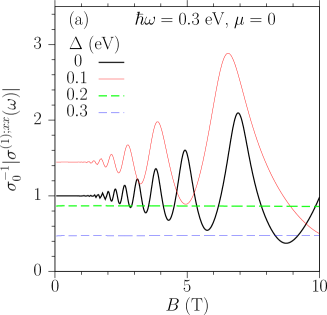
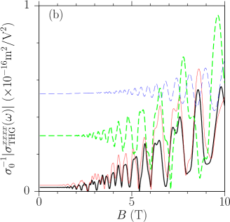
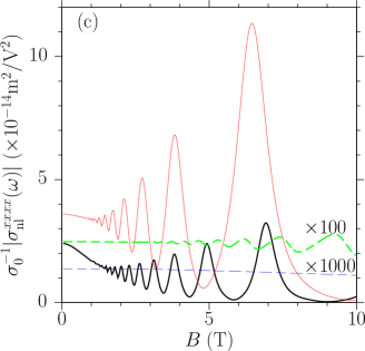
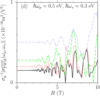
Figure 5: (color online) Magnetic field dependence of the absolute values of optical conductivities of GG. (a) $|\sigma^{(1);xx})\omega)|$, (b) $|\sigma^{xxxx}_{\text{THG}}(\omega)|$, (c) $|\sigma^{xxxx}_{\text{nl}}(\omega)|$, (d) $|\sigma^{xxxx}_{\text{FWM}}(\omega_{p},\omega_{s})|$. The parameters are $\hbar\omega=\hbar\omega_{s}=0.3$ eV, $\hbar\omega_{p}=0.5$ eV, $\Gamma=10$ meV, $\mu=0$, and $T=10$ K. In (b), the curves for $\Delta=0.2$ and $0.3$ eV are scaled by 100 and 1000 times, respectively.

ant. These features are understood as follows.

The peaks of the conductivity are induced by the resonant transitions. Based on the energy factor in Eq. (27), the resonant conditions can be summarized as ${\cal E}_{s_{1}s_{2}}(\epsilon,n,m)=0$, where $\epsilon$ is a transition energy. Around the resonance, the conductivity behaves as a Lorentz type divergence $[{\cal E}_{s_{1}s_{2}}(\epsilon+\delta E+i\Gamma,n,m)]^{-1}$ with respect to $\delta E$. For GG, we find that only the interband transitions lead to resonances, under the condition

$$\epsilon_{n+m}+\epsilon_{n}=\epsilon\,.$$ (41)

Here $n$ is a Landau index varying freely, $(m,\epsilon)$ can be used to identify channel for resonant optical transition. From Eq. (41) the magnetic field can be solved as $B={\cal B}_{e}(\epsilon,n,m)$ with

$${\cal B}_{e} (\epsilon,n,m)=\frac{\epsilon^{2}-(2\Delta)^{2}}{2e\hbar v_{F}^{2}}$$ (42)

$$\times\left[(2n+m)+2\sqrt{n(n+m)+m^{2}\left(\frac{\Delta}{\epsilon}\right)^{2}}\right]^{-1}\,.\quad$$

This solution exists only for $w>2\Delta$, where the photon energy is higher than the energy gap and the interband transitions could be in resonance. The function ${\cal B}_{e}(\epsilon,n,m)$ decreases with $n$, $m$, and $\Delta$, but increases with $\epsilon$. For a fixed channel $(m,\epsilon)$, the resonant transitions induced by the Landau index $n$ occur at the field ${\cal B}_{e}(\epsilon,n,m)$. For large $n$ or $m=0$, $[{\cal B}_{e}(\epsilon,n,m)]^{-1}\propto n$ indicates that the conductivities are approximately periodic in $B^{-1}$, similar to that of de Haas-van Alphen effect; but for the resonance occurring between the lowest several Landau levels, the period is also affected by $m$ and $\Delta/\epsilon$, deviating from the periodicity with respect to $B^{-1}$. The neighboring resonant peaks in the same channel occur between the Landau indices $n$ and $n+1$. The period is then $\Delta B_{n}={\cal B}_{e}(\epsilon,n,m)-{\cal B}_{e}(\epsilon,n+1,m)$. At a large $n\gg m$, the period $\Delta B_{n}\approx-\partial_{n}{\cal B}_{e}(\epsilon,n,m)\approx{\cal B}_{e}(\epsilon,n,m)/n\propto n^{-2}$ decreases quickly with $n$. Therefore at weak magnetic field, the resonance occurs at large $n$, and it is easier to smear out the oscillations, as shown in the region for $B<B_{c}$. However, when there exist multiple resonant channels, their oscillations are mixed and complicated.

We identify the resonant channels. For the linear conductivity, there is only one channel as $(m,\epsilon)=(1,\hbar\omega)$. The resonant magnetic field is given by $B_{1}={\cal B}_{e}(\hbar\omega,n,1)$.

n	0	1	2	3	4	5
$\Delta=0~{}~{}$ eV	68.3	11.7	6.9	4.9	3.8	3.1
$\Delta=0.1$ eV	22.8	6.4	3.8	2.7	2.1	1.7

Table 1: Magnetic field ${\cal B}_{e}(0.3,n,1)$ for different $n$.

In Table 1 we list the values for first several $n$ at $\Delta=0$ and $0.1$ eV. These values agree with the peak positions shown in Fig. 5 (a). For $\Delta\geq 0.15$ eV, there is no interband resonant transitions and thus no oscillations, as shown in Fig. 5 (a).

For the nonlinear conductivities, each denominator includes three energy factors, and there are multiple resonant channels. In some special conditions, it is possible to have more than one of these channels occurring simultaneously. For THG, these channels include $(m,\epsilon)=(1,\hbar\omega)$, $(0,2\hbar\omega)$, $(2,2\hbar\omega)$, and $(1,3\hbar\omega)$. They lead to the following types of divergences

$$\begin{array}[]{rlcl}&[{\cal E}_{+-}(\hbar\omega+i0^{+},n,1))]^{-1}\,,&&[{\cal E}_{+-}(2\hbar\omega+i0^{+},n,0)]^{-1}\,,\\ &[{\cal E}_{+-}(2\hbar\omega+i0^{+},n,2)]^{-1}\,,&&[{\cal E}_{+-}(3\hbar\omega+i0^{+},n,1)]^{-1}\,.\end{array}$$

The magnetic fields for these four channels are $B_{1}={\cal B}_{e}(\hbar\omega,n,1)$, $B_{2}={\cal B}_{e}(2\hbar\omega,n,0)$, $B_{3}={\cal B}_{e}(2\hbar\omega,n,2)$, and $B_{4}={\cal B}_{e}(3\hbar\omega,n,1)$. For $\Delta=0.3$ eV, only the channel $B_{4}$ exists. Because the relevant energy is $3\hbar\omega$, the resonant levels have larger index $n$ than those of the linear conductivity. Inside $[0,10]$ T, the resonant magnetic fields are $9.0$, $8.2$, $7.4$, $6.8$, $6.3$ T, $\cdots$ for $n=8$, $9$, $10$, $11$, $12$, $\cdots$, respectively. The periods of this channel are shorter than that of the channel $(m,\epsilon)=(1,\hbar\omega)$ in linear conductivity. For $\Delta=0.2$ eV, the extra channels $B_{2}$ and $B_{3}$ are added, and lead to the complicated resonances. The fields for resonant transitions can be easily identified by using Eq. (42) and we do not present them here. Similar results are found for $\Delta=0.1$ eV and $\Delta=0$, where all channels are possible. Interestingly, at weak magnetic field, these resonant transitions contribute to the THG conductivity destructively, where the two-photon resonant transitions contribute with a sign opposite to those from one- and three-photon resonant transitions. Their cancellation leads to a small THG conductivity for cases $\Delta=0.0$ and $0.1$ eV. When the magnetic field is strong, the nonequidistant LLs affect the electronic states at low energies more than those at high energies. Therefore, the magnetic field affects one-photon resonant transition more than the other two transitions, and breaks the cancellation to induce an increment up to 20 times for the THG conductivity.

For NL, the possible resonant channels are $(m,\epsilon)=(1,\hbar\omega)$, $(0,2\hbar\omega)$, and $(2,2\hbar\omega)$. They lead to the following divergences

$$\begin{array}[]{rlcl}&[{\cal E}_{+-}(\hbar\omega+i0^{+},n,1)]^{-2}\,,&&[{\cal E}_{+-}(\hbar\omega+i0^{+},n,1)]^{-1}\,,\\ &[{\cal E}_{+-}(\hbar\omega-i0^{+},n,1)]^{-1}\,,&&[{\cal E}_{+-}(2\hbar\omega+i0^{+},n,0)]^{-1}\,,\\ &[{\cal E}_{+-}(2\hbar\omega+i0^{+},n,2)]^{-1}\,.\end{array}$$

There also exists energy factors like $(i0^{+})^{-1}$ and $(2\hbar\omega+i0^{+})^{-1}$. However, neither of them lead to any divergence. There exist several resonant channels, but the one involving ${\cal B}_{e}(\hbar\omega,n,1)$ leads to resonances with higher order divergence ($[{\cal E}_{+-}(\hbar\omega+i0^{+},n,1)]^{-2}$) and is dominant. Thus at $\Delta=0$ and $0.1$ eV, although all channels are possible, the higher order divergence dominates, which is induced by the same resonant channel as that of linear conductivity. It is not surprising that these spectra have the same oscillations as those of linear conductivity. For $\Delta=0.2$ eV, the linear conductivity does not have an available channel, and this higher order divergence channel for NL is also forbidden. However, for NL the other two channels are available. For magnetic field in the range of $[0,10]$ T, the resonant magnetic fields for the channel $(m,\epsilon)=(0,2\hbar\omega)$ are $9.5$, $7.6$, $6.3$, $5.4$, $4.7$, $4.2$ T, $\cdots$ for $n=4$, $5$, $6$, $7$, $8$, $9$, $\cdots$, respectively; those for the channel $(m,\epsilon)=(2,2\hbar\omega)$ are $9.6$, $7.6$, $6.3$, $5.4$, $4.7$, $4.2$ T, $\cdots$ for $n=3$, $4$, $5$, $6$, $7$, $8$, $\cdots$, respectively. The period for $\Delta=0.2$ eV is shorter than those of $\Delta=0$ and $0.1$ eV. For $\Delta=0.3$ eV, no channel is available, and the conductivity shows no oscillations.

For FWM, two frequencies $\omega_{p}$ and $\omega_{s}$ can result in more channels $(m,\epsilon)=(1,\hbar\omega_{s})$, $(1,\hbar\omega_{p})$, $(0,\epsilon_{a})$, $(2,\epsilon_{a})$, $(0,2\hbar\omega_{p})$, $(2,2\hbar\omega_{p})$, and $(1,\epsilon_{b})$ with $\epsilon_{a}=\hbar\omega_{p}-\hbar\omega_{s}$ and $\epsilon_{b}=2\hbar\omega_{p}-\hbar\omega_{s}$. They lead to the following divergences

$$\begin{array}[]{clcl}&[{\cal E}_{+-}(\hbar\omega_{s}-i0^{+},n,1]^{-1}\,,&&[{\cal E}_{+-}(\hbar\omega_{p}+i0^{+},n,1)]^{-1}\,,\\ &[{\cal E}_{+-}(\epsilon_{a}+i0^{+},n,0)]^{-1}\,,&&[{\cal E}_{+-}(\epsilon_{a}+i0^{+},n,2)]^{-1}\,,\\ &[{\cal E}_{+-}(2\hbar\omega_{p}+i0^{+},n,0)]^{-1}\,,&&[{\cal E}_{+-}(2\hbar\omega_{p}+i0^{+},n,2]^{-1}\,,\\ &[{\cal E}_{+-}(\epsilon_{b},n,1)]^{-1}\,.\end{array}$$

In the limit $\omega_{s}=\omega_{p}$, the FWM conductivity is reduced to that of the NL conductivity, and the higher order divergence $(\delta E+i0^{+})^{-2}$ is a combination of two energy factors. We take the case $\Delta=0.3$ eV as an example. The resonances can be induced by the energy factors ${\cal E}_{+-}(2\hbar\omega_{p}+i0^{+},n,0)$, ${\cal E}_{+-}(2\hbar\omega_{p}+i0^{+},n,0)$, and ${\cal E}_{+-}(\epsilon_{b}+i0^{+},n,1)]^{-1}$. For $B\in[0,10]$ T, the resonant magnetic field ${\cal B}_{e}(\epsilon_{b},n,1)$ is $9.9$, $7.1$, $5.5$, and $4.5$ for $n=2$, $3$, $4$, and $5$, respectively. These field values determine the main peaks. The fields ${\cal B}_{e}(2\hbar\omega_{p},n,0)$ and ${\cal B}_{e}(2\hbar\omega_{p},n-1,2)$ are very close with values around $9.35$, $8.68$, $8.1$, and $7.6$ for $n=13$, $14$, $15$, and $16$, respectively. These field values determine the small changes on both sides of the main peaks. Other peaks can be understood in a similar fashion.

IV.2 Results of DG

In Fig. 6, we present the absolute values of conductivities $\sigma^{(1);xx}(\omega)$, $\sigma^{xxxx}_{\text{nl}}(\omega)$, $\sigma^{xxxx}_{\text{THG}}(\omega)$, and $\sigma^{xxxx}_{\text{FWM}}(\omega_{p},\omega_{s})$ of DG at the chemical potential $\mu=0$, $-0.1$, $-0.2$, and $-0.3$ eV, by varying the magnetic field $B$ from $0$ to $10$ T. Because of the finite doping, the transverse conductivity components $\sigma^{(1);xy}$, $\sigma^{(3);xyxx}$, $\sigma^{(3);xxyx}$, and $\sigma^{(3);xxxy}$ are nonzero.

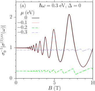
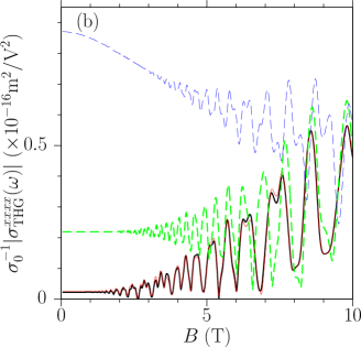
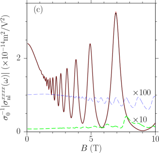
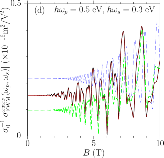
Figure 6: (color online) Magnetic field dependence of the absolute values of optical conductivities of DG (a) $|\sigma^{(1);xx}(\omega)|$, (b) $|\sigma^{xxxx}_{\text{THG}}(\omega)|$, (c) $|\sigma^{xxxx}_{\text{nl}}(\omega)|$, (d) $|\sigma^{xxxx}_{\text{FWM}}(\omega_{p},\omega_{s})|$. The parameters are $\hbar\omega=\hbar\omega_{s}=0.3$ eV, $\hbar\omega_{p}=0.5$ eV, $\Gamma=10$ meV, $\Delta=0$, and $T=10$ K. In (c), the curves for $\mu=-0.2$ and $-0.3$ eV are scaled by 10 and 100 times, respectively.

In the limit of zero magnetic field, the chemical potential dependence of the conductivities has been discussed in literature and also shown in Fig. 4. The effect of the chemical potential is very similar to an energy gap, but they also have essential differences. With increasing the magnetic field, the conductivities at all chemical potentials oscillate. Compared to the conductivities of GG, the optical response of DG shows some different magnetic field dependence: (1) As opposed to the gap parameter dependence, the conductivities have little difference for $\mu=0$ and $-0.1$ eV. All the photon energies we calculated are away from resonance for these two chemical potentials. (2) It can be seen that for a given resonant channel the oscillation period does not depend on the chemical potential. (3) At $\mu=-0.2$ and $-0.3$ eV, $\sigma^{(1);xx}$ and $\sigma^{xxxx}_{\text{nl}}$ show additional fluctuations. They are induced by the difference between the left and right circularly polarized components. In the dc limit, $\sigma^{(1);xy}$ is induced by quantum Hall effects, and its value is determined by the number of doped LLs and shows one plateau for each LL. Similar natures also exist in the longitudinal components and lead to such plateau like fluctuations.

In contrast to the undoped case in GG, where the resonance occur only between the interband transitions, here resonant intraband transitions are also possible. For DG, the values for all possible magnetic fields are given by

$${\cal B}_{s}(\epsilon,n,m) = \frac{\epsilon^{2}}{2e\hbar v_{F}^{2}}\frac{1}{(\sqrt{n+m}+s\sqrt{n})^{2}}$$ (43)

$$\approx 760\left(\frac{\epsilon}{\text{eV}}\right)^{2}\frac{1}{(\sqrt{n+m}+s\sqrt{n})^{2}}\,,$$

with $s=-1$ for resonant intraband transitions and $s=1$ for resonant interband transitions. A simple calculation shows that there is no resonant intraband transition for the photon frequencies considered and the magnetic field in the range of $[0,10]$ T. Thus only the resonant interband transitions are possible in our parameters. The chemical potential does not affect the value of the resonant magnetic field, but it can block some channels for a number of Landau index $n$. This can be clearly seen from the conductivity $\sigma^{(1);xx}(\omega)$ at $\mu=0$, $-0.1$, and $-0.2$. The energy of involved electron/hole in the resonant transition can be approximated as $\pm\hbar\omega/2\sim\pm 0.15$ eV. At room temperature $T=300$ K, both the electron and hole are almost empty for the case $\mu=-0.3$ eV, which lead to

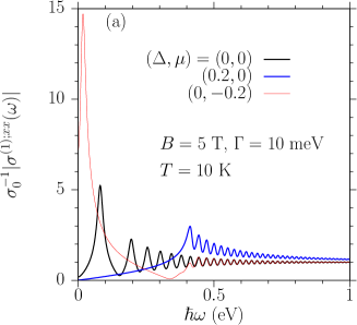
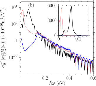
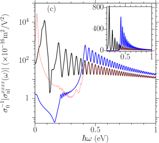
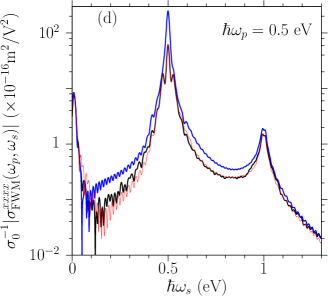
Figure 7: (color online) Spectra of absolute values of optical conductivities of GG and DG at $B=5$ T for different chemical potential and gap parameter $(\Delta,\mu)$. (a) $|\sigma^{(1);xx}(\omega)|$, (b) $|\sigma^{xxxx}_{\text{THG}}(\omega)|$, (c) $|\sigma^{xxxx}_{\text{nl}}(\omega)|$, (d) $|\sigma^{xxxx}_{\text{FWM}}(\omega_{p},\omega_{s})|$. The gap parameter and the chemical potential are $(\Delta,\mu)=(0,0)$, $(0.2,0)$, and $(0,-0.2)$ eV. Other parameters are $\hbar\omega_{p}=0.5$ eV, $\Gamma=10$ meV, and $T=10$ K. The inset in (b) gives the details at low photon energy $\hbar\omega\in[0,0.15]$ eV, and that in (c) gives the details at high photon energy $\hbar\omega\in[0.15,1]$ eV; both $y$-axes are in linear scale. The $y$-axes of the main diagrams of (b), (c), and (d) are in logarithmic scale.

the vanishing of the resonant interband transition. Similar results can be found for $\sigma^{xxxx}_{\text{nl}}(\omega)$. For the nonlinear conductivities, the occupation of levels only affects the transition involving $w_{3}$ in Fig. 2. Because some channels are determined by more than one resonant transition, it is not a surprise that the resonant peaks of $\sigma^{xxxx}_{\text{THG}}$ and $\sigma^{xxxx}_{\text{FWM}}$ are so complicated.

V Optical conductivities at strong magnetic field

In this section we present the conductivities at a strong magnetic field $B=5$ T. The cyclotron energy is $\hbar\omega_{c}=81$ meV, from which the lowest several energy levels are $\epsilon_{n}=0$, $81$, $114$, $140$, $162$, $181$ meV at $n=0,1,2,3,4,5$ for $\Delta=0$ and $\epsilon_{n}=0.2$, $0.216$, $0.230$, $0.244$, $0.257$ at $n=0,1,2,3,4,5$ for $\Delta=0.2$. Both cases show explicit discrete levels. Our numerical results are shown in Fig. 7 for $\sigma^{(1);xx}(\omega)$, $\sigma^{xxxx}_{\text{THG}}(\omega)$, $\sigma^{xxxx}_{\text{nl}}(\omega)$, and $\sigma^{xxxx}_{\text{FWM}}(\omega_{p},\omega_{s})$ at three different chemical potentials and gap parameters $(\Delta,\mu)=(0,0)$, $(0.2,0)$, and $(0,-0.2)$ eV, which are noted as intrinsic graphene (IG), GG, and DG in the following.

The linear conductivity is plotted in Fig. 7 (a). All spectra show oscillations. For photon energies $\hbar\omega>0.4$ eV, the oscillations are similar for all three cases. With the increase of the photon energy, the oscillation period and amplitude decrease. From our results in previous sections, we understand these oscillations from the resonant interband transitions for $\hbar\omega>E_{g}$, which occur between the electronic state “$sn$”$=$“$-n$” and the state “$+(n+1)$” or between “$-(n+1)$” and “$+n$”. The peak positions are determined by the transition energy $\hbar\omega=\epsilon_{n+1}+\epsilon_{n}$, with $n\geq 0$ for GG and $n\geq 6$ for IG and DG. In this region, the conductivity oscillates around the value of conductivity at zero magnetic field. Furthermore, the cases for IG and DG are almost identical, because they have the same optical resonant transitions between the same LLs. When the photon energy $\hbar\omega<0.4$ eV, the conductivities show different behavior. For the case of IG, the interband resonant transitions can be extended to $n=1$; while the special case at $n=0$, corresponding to a transition energy $\hbar\omega=81$ meV, includes both intraband and interband transitions. For the case of DG, the interband transitions are blocked; however, there is one extra peak at $18$ meV. This peak results from the intraband transition between LLs of “$-(n+1)$” and “$-n$” at $n=6$. It is the modified Drude contribution for LLs. For the case of GG, all interband transitions are forbidden, and they result in a smooth linear conductivity. The spectrum of $\sigma^{xxxx}_{\text{nl}}(\omega)$ in Fig. 7 (c) shows dependence on photon energy similar to that of the linear conductivity.

The spectra of THG conductivity $\sigma^{xxxx}_{\text{THG}}(\omega)$ are shown in Fig. 7 (b). For $\hbar\omega$ less than about $0.15$ eV, the spectra of the conductivity include a few peaks for IG and DG, and the values can be as large as $5\times 10^{-13}\sigma_{0}\text{V}^{2}/\text{m}^{2}$. The peaks locate at around $8$, $27$, and $64$ meV for IG, and $4$ and $14.5$ meV for DG. By checking the energies for interband resonant transitions and possible intraband resonant transitions, the peak at $64$ meV is induced by the three-photon resonant interband transitions between “$-1$” and “$+2$” or between “$-2$” and “$+1$”; the peaks at $27$ meV or $8$ meV are induced by resonant intraband transitions, between the LLs around the Fermi surface. From the illustration diagrams listed in Fig. 2, the resonant transitions can occur at any stage of the three transitions; some of them have no requirement for the occupation of the initial and final states. However, the dominant contributions are still from the resonant transitions from an occupied state to an empty state. A similar analysis can be applied to the case of DG, where the first two peaks comes from the intraband transitions around $n=6$. For higher photon energies, many oscillations appear; they are induced by interband transitions, as discussed in previous section. Even at very high photon energies, the conductivity can be tuned by about two orders of magnitude in one oscillation. Because LLs are nonequidistant, the resonant transitions at high photon energies involve very high LL indices, where the magnetic field only modulates the original band structure slightly. Therefore, similar to that of graphene without the presence of a magnetic field, the conductivity decreases as power law of frequency for high photon energies Cheng et al. (2014), but modulated by oscillations from the LLs.

The spectra of the conductivity of FWM process $\sigma^{xxxx}_{\text{FWM}}(\omega_{p},\omega_{s})$ are plotted in Fig. 7 (d). It keeps the features of the results at zero magnetic field, and it shows three resonant peaks at $\hbar\omega_{s}=0$, $\hbar\omega_{p}$, and $2\hbar\omega_{p}$. The first is induced by the Drude-like contributions. At the second one, the FWM process is reduced to NL process. Because the one-photon absorption exists in our parameters, the two-photon absorption process diverges, and the conductivity exhibits a divergent peak. At the third one, the FWM process corresponds to a current injection process, which diverges too. However, although the magnetic field modulates the conductivity, the changes are smaller than those in the conductivities for THG and NL processes.

Here we note that the resonant intraband transitions give huge responses, similar to their contributions at zero magnetic field. However, the magnetic field brings an advantage for controlling the position of resonant peak, from $\hbar\omega=0$ at zero magnetic field to a nonzero value for nonzero magnetic field.

VI Conclusion

In this work, we have investigated the perturbative linear and third order conductivities of gapped graphene and doped graphene in the presence of a perpendicular magnetic field. The electron dynamics are solved from the equation of motion using Landau levels. The light matter interaction is described in the length gauge and the scattering is included in a phenomenological way with only one relaxation parameter. We discuss the nonlinear processes for third harmonic generation, the nonlinear corrections to the linear conductivity, and four wave mixing.

We first show that the Landau levels form a good basis functions even at very weak magnetic field, which can be used to calculate the conductivities of systems without magnetic field. We apply this approach to a doped graphene and the results agree with the calculation from an analytic expression in literature. Using the same approach, we present the optical conductivities of a gapped graphene. Similar to the chemical potential related resonant transition in doped graphene, there exist energy gap related resonant transitions, occurring when any of the involved photon energies matches the band gap. The main difference lies in the absence of the Drude contribution in a gapped graphene, which leads to its temperature insensitivity and dielectric nature below the band gap.

At strong magnetic fields, the Landau levels are discrete and there exist many resonant transitions. Varying the magnetic field in the range of $[0,10]$ T, the nonlinear conductivity can be tuned up to $1-2$ orders of magnitude. There exist different resonant channels, especially in the nonlinear optical response. Some of them can be turned on and off by tuning the the gap parameter and the chemical potential, leading to different oscillation features. We also present a simple condition to identify these resonant transitions. We calculate the spectra of these conductivities at strong magnetic field. The spectra show oscillations, which are induced by the resonant transitions between different Landau levels. At small photon energies, the conductivity of DG show peaks due to the resonant intraband transitions, corresponding to a modified Drude contribution.

In our calculations, the phenomenological relaxation time approximation is a very rough treatment, which is intended to describe all microscopic relaxation processes, many-body effects, and thermal effects in just one parameter. For optical properties in most materials, such treatment will not lead to difficulties because the time scale of optical field is much faster than the scattering processes, and such a treatment is mostly used to remove the divergence in the calculation. Although it is not clear whether or not this is still the case for graphene in a strong magnetic field, the calculation presented here can at least indicates interesting qualitative behavior at the considered frequencies and field strengths, such as the oscillations and the dependence on the gap parameter and chemical potentials. These properties are likely to remain in more sophisticated calculations. Because all these oscillations can be tuned by the strength of the magnetic field, these calculations indicate a new way to control the optical response in the terahertz to the far-infrared.

To connect with experiments like four wave mixing and third harmonic generation, it might be convenient to estimate the output intensity from the input ones. For free-standing graphene, the radiated electric field can be calculated Yao and Belyanin (2012); Boyd (2008) by $E^{x}(2\omega_{1}+\omega_{2})|\approx\sigma^{(3);xxxx}(\omega_{1},\omega_{1},\omega_{2})/(2c\epsilon_{0})[E^{x}(\omega_{1})]^{2}E^{x}(\omega_{2})$, and then the output intensity $I(2\omega_{1}+\omega_{2})$ is given by

$$I(2\omega_{1}+\omega_{2}) \approx \frac{|\sigma^{(3);xxxx}(\omega_{1},\omega_{1},\omega_{2})|^{2}}{(2c\epsilon_{0})^{4}}[I(\omega_{1})]^{2}[I(\omega_{2})]$$ (44)

$$\approx 46.6\left|\frac{\sigma^{(3);xxxx}(\omega_{1},\omega_{1},\omega_{2})}{10^{-14}\sigma_{0}}\right|^{2}$$

$$\times\left[\frac{I(\omega_{1})}{1\text{GW/m}^{2}}\right]^{2}\left[\frac{I(\omega_{2})}{1\text{GW/m}^{2}}\right]\,.$$

The output intensity is directly determined by the square of the conductivity. For fixed input laser pulse, the maximal output intensity can be found when the conductivities are maximized by tuning the magnetic field and the gap parameter/chemical potential. If the graphene is inside a complicated structure, the output can be strongly modified by the design of the structure.

Appendix A Matrix elements of position and velocity operators

Because there is no coupling between different valleys, the position and velocity operators only have matrix elements between the electronic states in the same valley. The matrix elements of position operators are given as

$$\int d\bm{r}\Psi_{\nu s_{1}n_{1}k_{1}}^{{\dagger}}(\bm{r})x\Psi_{\nu s_{2}n_{2}k_{2}}(\bm{r})$$

$$=\delta(k_{1}-k_{2})\left(\xi_{\nu;s_{1}n_{1},s_{2}n_{2}}^{x}-l_{c}^{2}k_{2}\delta_{s_{1},s_{2}}\delta_{n_{1},n_{2}}\right)\,,$$ (45)

$$\int d\bm{r}\Psi_{\nu s_{1}n_{1}k_{1}}^{{\dagger}}(\bm{r})y\Psi_{\nu s_{2}n_{2}k_{2}}(\bm{r})$$

$$=\delta(k_{1}-k_{2})\xi_{\nu;s_{1}n_{1},s_{2}n_{2}}^{y}-i\frac{\partial\delta(k_{1}-k_{2})}{\partial k_{2}}\delta_{s_{1},s_{2}}\delta_{n_{1},n_{2}}\,,\quad$$ (46)

with

$$\xi_{\nu;s_{1}n_{1},s_{2}n_{2}}^{x} = \int dx\Phi_{\nu s_{1}n_{1}}^{{\dagger}}(x)x\Phi_{\nu s_{2}n_{2}}(x)\,,$$

$$\xi_{\nu;s_{1}n_{1},s_{2}n_{2}}^{y} = -\frac{l_{c}^{2}}{\hbar}\int dx\Phi_{\nu s_{1}n_{1}}^{{\dagger}}(x)p_{x}\Phi_{\nu s_{2}n_{2}}(x)\,.$$

Further the circularly polarized components are

$$\xi_{\nu;s_{1}n_{1},s_{2}n_{2}}^{+} = -il_{c}\int dx\Phi_{\nu s_{1}n_{1}}^{{\dagger}}(x)\hat{a}^{\dagger}\Phi_{\nu s_{2}n_{2}}(x)\,,$$

$$\xi_{\nu;s_{1}n_{1},s_{2}n_{2}}^{-} = ~{}~{}il_{c}\int dx\Phi_{\nu s_{1}n_{1}}^{{\dagger}}(x)\hat{a}\Phi_{\nu s_{2}n_{2}}(x)$$ (47)

$$= (\xi_{\nu;s_{2}n_{2},s_{1}n_{1}}^{+})^{\ast}\,.$$

Using the properties of the operator in Eq. (7), we can get Eq. (17). Using the symmetry between two valleys in Eq. (4), we verify

$$\xi^{\tau}_{\nu;s_{1}n_{1},s_{2}n_{2}}=s_{1}s_{2}\xi^{\tau}_{\overline{\nu};\overline{s}_{1}n_{1},\overline{s}_{2}n_{2}}\,.$$ (48)

Therefore, the values of all $\xi^{\tau}_{\nu;s_{1}n_{1},s_{2}n_{2}}$ can be generated from $\xi^{+}_{+;s_{1}(n+1),s_{2}n}$ by Eqs. (47) and (48).

The velocity operator is $\bm{v}_{\nu}=[\bm{r},H_{\nu;p+e\bm{A}(\bm{r})}]/(i\hbar)$. Because the level energy is independent of $k$, it is calculated directly to give

$$\int d\bm{r}\Psi_{\nu s_{1}n_{1}k_{1}}^{{\dagger}}(\bm{r})\bm{v}_{\nu}\Psi_{\nu s_{2}n_{2}k_{2}}(\bm{r})=\delta(k_{1}-k_{2})\bm{v}_{\nu;s_{1}n_{1},s_{2}n_{2}}\,,$$

with

$$\bm{v}_{\nu;s_{1}n_{1}.s_{2}n_{2}}=i\hbar^{-1}(s_{1}\epsilon_{n_{1}}-s_{2}\epsilon_{n_{2}})\bm{\xi}_{\nu;s_{1}n_{1},s_{2}n_{2}}\,.$$

In Fig. 8 we give $i\xi_{+;s_{1}(n+1),s_{2}n}^{+}$ and $v_{+;s_{1}(n+1),s_{2}n}^{+}$ for different $n$ and $s_{i}$. For the special term $n=0$, we have $\xi^{+}_{+;s_{1}1,s_{2}0}=-il_{c}\sqrt{1-s_{1}\alpha_{1}}/\sqrt{2}\delta_{s_{2},-1}$. The optical dipole matrix elements between the same bands ($s_{1}s_{2}=1$) have larger values which increase with $n$. The interband matrix elements ($s_{1}s_{2}=-1$) have smaller values: $\xi_{+;+(n+1),-n}^{+}$ decreases with $n$; $\xi_{+,-(n+1),+n}^{+}$ first increases then decreases, where there exists a maximum value depending on the ratio $\Delta/\hbar\omega_{c}$. For the velocity matrix elements, both intraband and interband terms have similar amplitude. For graphene, they have the values $v_{+;+(n+1),sn}^{+}=-v_{+;-(n+1),sn}^{+}=v_{F}/\sqrt{2}$ for all $n\geq 1$ and $v_{+;s_{1}1,s_{2}0}^{+}=s_{1}v_{F}\delta_{s_{2},-1}$.

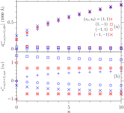
Figure 8: (color online) The landau level index dependence of (a) $i\xi_{+;s_{1}(n+1),s_{2}n}^{+}$ and (b) $v_{+;s_{1}(n+1),s_{2}n}^{+}$ for $B=1$ T and $\Delta=0$ (red symbols) and $\Delta=0.1$ eV (blue symbols).

Appendix B Perturbative optical conductivities

For a weak electric field, Eq. (21) can be solved perturbatively by expanding $\rho_{\nu}(t)$ up to the third order of the electric field as

$$\rho_{\nu}(t) = \rho^{0}_{\nu}+\int\frac{d\omega_{3}}{2\pi}\widetilde{\cal P}^{(1);\gamma}_{\nu}(w_{3})E^{\overline{\gamma}}({\omega_{3}})e^{-i\omega_{3}t}$$ (49)

$$+ \int\frac{d\omega_{2}d\omega_{3}}{(2\pi)^{2}}\widetilde{\cal P}_{\nu}^{(2);\beta\gamma}(w_{0},w_{3})E^{\overline{\beta}}({\omega_{2}})E^{\overline{\gamma}}({\omega_{3}})e^{-i(\omega_{2}+\omega_{3})t}$$

$$+ \int\frac{d\omega_{1}d\omega_{2}d\omega_{3}}{(2\pi)^{3}}\widetilde{\cal P}_{\nu}^{(3);\alpha\beta\gamma}(w,w_{0},w_{3})E^{\overline{\alpha}}({\omega_{1}})E^{\overline{\beta}}({\omega_{2}})$$

$$\times E^{\overline{\gamma}}({\omega_{3}})e^{-i(\omega_{1}+\omega_{2}+\omega_{3})t}+\cdots$$

where $E^{\alpha}({\omega})=\int dtE^{\alpha}(t)e^{i\omega t}$ is the Fourier transform of the field $E^{\alpha}(t)$, $w_{3}=\hbar\omega_{3}+i\Gamma$, $w_{0}=\hbar(\omega_{2}+\omega_{3})+i\Gamma$, $w=\hbar(\omega_{1}+\omega_{2}+\omega_{3})+i\Gamma$; the dependence on $w_{3}$, $w_{0}$, and $w$ is clear from the following expressions. Substituting the expansion above into Eq. (21) and comparing the terms with the same order of electric field at both sides, we get

$$\widetilde{\cal P}_{\nu;s_{1}n_{1},s_{2}n_{2}}^{(1);\gamma}(w_{3}) = \frac{e\xi^{\gamma}_{\nu;s_{1}n_{1},s_{2}n_{2}}(f_{s_{2}n_{2}}-f_{s_{1}n_{1}})}{w_{3}-(s_{1}\epsilon_{n_{1}}-s_{2}\epsilon_{n_{2}})}\,,$$ (50)

$$\widetilde{\cal P}_{\nu;s_{1}n_{1},s_{2}n_{2}}^{(2);\beta\gamma}(w_{0},w_{3}) = \frac{[e\xi^{\beta}_{\nu},\widetilde{\cal P}_{\nu}^{(1);\gamma}(w_{3})]_{s_{1}n_{1},s_{2}n_{2}}}{w_{0}-(s_{1}\epsilon_{n_{1}}-s_{2}\epsilon_{n_{2}})}\,,$$ (51)

$$\widetilde{\cal P}_{\nu;s_{1}n_{1},s_{2}n_{2}}^{(3);\alpha\beta\gamma}(w,w_{0},w_{3}) = \frac{[e\xi^{\alpha}_{\nu},\widetilde{\cal P}_{\nu}^{(2);\beta\gamma}(w_{0},w_{3})]_{s_{1}n_{1},s_{2}n_{2}}}{w-(s_{1}\epsilon_{n_{1}}-s_{2}\epsilon_{n_{2}})}\,.\quad~{}$$ (52)

The total current density is given as $\bm{J}(t)=\langle\hat{\bm{J}}(t)\rangle=J^{\alpha}\hat{\bm{e}}^{\overline{\alpha}}$ with

$$J^{\alpha}(t)=-e{\cal D}\sum_{\tau s_{1}s_{2}\atop n_{1}n_{2}}v^{\alpha}_{\tau;s_{2}n_{2},s_{1}n_{1}}\rho_{\tau;s_{1}n_{1},s_{2}n_{2}}(t)\,.$$ (53)

Correspondingly, the optical current can be expanded as $J^{\delta}(t)=J^{(1);\delta}(t)+J^{(3);\delta}(t)+\cdots$ with

$$J^{(1);\tau}(t) = \int\frac{d\omega_{3}}{2\pi}{\sigma}^{(1);\tau\gamma}(\omega_{3})E^{\gamma}({\omega_{3}})e^{-i\omega_{3}t}\,,$$ (54)

$$J^{(3);\tau}(t) = \int\frac{d\omega_{1}d\omega_{2}d\omega_{3}}{(2\pi)^{3}}\widetilde{\sigma}^{(3);\tau\alpha\beta\gamma}(w,w_{0},w_{3})E^{{\alpha}}({\omega_{1}})$$ (55)

$$\times E^{{\beta}}({\omega_{2}})E^{{\gamma}}({\omega_{3}})e^{-i(\omega_{1}+\omega_{2}+\omega_{3})t}\,,$$

where

$$\sigma^{(1);\tau\alpha}(\omega) = -e{\cal D}\sum_{\tau s_{1}s_{2}\atop n_{1}n_{2}}v^{\tau}_{\nu;s_{2}n_{2},s_{1}n_{1}}$$ (56)

$$\times\widetilde{\cal P}^{(1);\overline{\alpha}}_{\nu;s_{1}n_{1},s_{2}n_{2}}(\hbar\omega+i\Gamma)\,,$$

$$\widetilde{\sigma}^{(3);\tau\alpha\beta\gamma}(\omega_{1},\omega_{2},\omega_{3}) = -e{\cal D}\sum_{\tau s_{1}s_{2}\atop n_{1}n_{2}}v^{\tau}_{\nu;s_{2}n_{2},s_{1}n_{1}}$$ (57)

$$\times\widetilde{\cal P}^{(3);\overline{\alpha}\overline{\beta}\overline{\gamma}}_{\nu;s_{1}n_{1},s_{2}n_{2}}(w,w_{0},w_{3})\,.$$

By substituting Eqs. (50-52) we obtain Eqs. (22) and (24) in the main text.

The independent Cartesian components of the third order conductivity $\widetilde{\sigma}^{(3);dabc}(\omega_{1},\omega_{2},\omega_{3})$ are expressed from the circularly polarized components $\widetilde{\sigma}^{(3);\delta\alpha\beta\gamma}(\omega_{1},\omega_{2},\omega_{3})$ as

$${}{\sigma}^{(3);xxyy} = {}{\sigma}^{(3);yyxx}$$

$$= \frac{1}{4}\sum_{\tau}\left({}{\sigma}^{(3);\tau\tau{\tau}\overline{\tau}}+{}{\sigma}^{(3);\tau{\tau}\overline{\tau}{\tau}}-{}{\sigma}^{(3);\tau\overline{\tau}{\tau}\tau}\right)\,,$$

$${}{\sigma}^{(3);xyxy} = {}{\sigma}^{(3);yxyx}$$

$$= \frac{1}{4}\sum_{\tau}\left({}{\sigma}^{(3);\tau\tau{\tau}\overline{\tau}}-{}{\sigma}^{(3);\tau{\tau}\overline{\tau}{\tau}}+{}{\sigma}^{(3);\tau\overline{\tau}{\tau}\tau}\right)\,,$$

$${}{\sigma}^{(3);xyyx} = {}{\sigma}^{(3);yxxy}$$

$$= \frac{1}{4}\sum_{\tau}\left(-{}{\sigma}^{(3);\tau\tau{\tau}\overline{\tau}}+{}{\sigma}^{(3);\tau{\tau}\overline{\tau}{\tau}}+{}{\sigma}^{(3);\tau\overline{\tau}{\tau}\tau}\right)\,,$$

and

$${}{\sigma}^{(3);xyxx} = -{}{\sigma}^{(3);yxyy}$$

$$= \frac{i}{4}\sum_{\tau}\tau\left({}{\sigma}^{(3);\tau\tau{\tau}\overline{\tau}}+{}{\sigma}^{(3);\tau{\tau}\overline{\tau}{\tau}}-{}{\sigma}^{(3);\tau\overline{\tau}{\tau}\tau}\right)\,,$$

$${}{\sigma}^{(3);xxyx} = -{}{\sigma}^{(3);yyxy}$$

$$= \frac{i}{4}\sum_{\tau}\tau\left({}{\sigma}^{(3);\tau\tau{\tau}\overline{\tau}}-{}{\sigma}^{(3);\tau{\tau}\overline{\tau}{\tau}}+{}{\sigma}^{(3);\tau\overline{\tau}{\tau}\tau}\right)\,,$$

$${}{\sigma}^{(3);xxxy} = -{}{\sigma}^{(3);yyyx}$$

$$= \frac{i}{4}\sum_{\tau}\tau\left(-{}{\sigma}^{(3);\tau\tau{\tau}\overline{\tau}}+{}{\sigma}^{(3);\tau{\tau}\overline{\tau}{\tau}}+{}{\sigma}^{(3);\tau\overline{\tau}{\tau}\tau}\right)\,.$$

References

- Bonaccorso et al. (2010) F. Bonaccorso, Z. Sun, T. Hasan, and A. C. Ferrari, Nat. Photon. 4, 611 (2010).
- Bao and Loh (2012) Q. Bao and K. P. Loh, ACS Nano 6, 3677–3694 (2012).
- Low and Avouris (2014) T. Low and P. Avouris, ACS Nano 8, 1086 (2014).
- Sun et al. (2016) Z. Sun, A. Martinez, and F. Wang, Nat. Photon. 10, 227 (2016).
- Ferrari et al. (2015) A. C. Ferrari, F. Bonaccorso, V. Fal'ko, K. S. Novoselov, S. Roche, P. Bøggild, S. Borini, F. H. L. Koppens, V. Palermo, N. Pugno, J. A. Garrido, R. Sordan, A. Bianco, L. Ballerini, M. Prato, E. Lidorikis, J. Kivioja, C. Marinelli, T. Ryhänen, A. Morpurgo, J. N. Coleman, V. Nicolosi, L. Colombo, A. Fert, M. Garcia-Hernandez, A. Bachtold, G. F. Schneider, F. Guinea, C. Dekker, M. Barbone, Z. Sun, C. Galiotis, A. N. Grigorenko, G. Konstantatos, A. Kis, M. Katsnelson, L. Vandersypen, A. Loiseau, V. Morandi, D. Neumaier, E. Treossi, V. Pellegrini, M. Polini, A. Tredicucci, G. M. Williams, B. H. Hong, J.-H. Ahn, J. M. Kim, H. Zirath, B. J. van Wees, H. van der Zant, L. Occhipinti, A. D. Matteo, I. A. Kinloch, T. Seyller, E. Quesnel, X. Feng, K. Teo, N. Rupesinghe, P. Hakonen, S. R. T. Neil, Q. Tannock, T. Löfwander, and J. Kinaret, Nanoscale 7, 4598 (2015).
- Glazov and Ganichev (2014) M. Glazov and S. Ganichev, Phys. Rep. 535, 101 (2014).
- Cheng et al. (2014) J. L. Cheng, N. Vermeulen, and J. E. Sipe, New J. Phys. 16, 053014 (2014); New J. Phys. 18, 029501 (2016).
- Cheng et al. (2015a) J. L. Cheng, N. Vermeulen, and J. E. Sipe, Phys. Rev. B 91, 235320 (2015a); Phys. Rev. B 93, 039904 (2016).
- Mikhailov (2016) S. A. Mikhailov, Phys. Rev. B 93, 085403 (2016).
- Mikhailov (2007) S. A. Mikhailov, Europhys. Lett. 79, 27002 (2007).
- Hendry et al. (2010) E. Hendry, P. J. Hale, J. Moger, A. K. Savchenko, and S. A. Mikhailov, Phys. Rev. Lett. 105, 097401 (2010).
- Vermeulen et al. (2016) N. Vermeulen, J. Cheng, J. E. Sipe, and H. Thienpont, IEEE Journal of Selected Topics in Quantum Electronics 22, 347 (2016).
- Yao and Belyanin (2012) X. Yao and A. Belyanin, Phys. Rev. Lett. 108, 255503 (2012).
- Tokman et al. (2013) M. Tokman, X. Yao, and A. Belyanin, Phys. Rev. Lett. 110, 077404 (2013).
- Yao and Belyanin (2013) X. Yao and A. Belyanin, J. Phys. Condens. Matter 25, 054203 (2013).
- Rao and Sipe (2012) K. M. Rao and J. E. Sipe, Phys. Rev. B 86, 115427 (2012).
- Brem et al. (2017) S. Brem, F. Wendler, and E. Malic, Phys. Rev. B 96, 045427 (2017).
- Goerbig (2011) M. O. Goerbig, Rev. Mod. Phys. 83, 1193 (2011).
- Gusynin et al. (2007) V. P. Gusynin, S. G. Sharapov, and J. P. Carbotte, J. Phys. Condens. Matter 19, 026222 (2007).
- Crassee et al. (2010) I. Crassee, J. Levallois, A. L. Walter, M. Ostler, A. Bostwick, E. Rotenberg, T. Seyller, D. van der Marel, and A. B. Kuzmenko, Nat. Phys. 7, 48 (2010).
- Pyatkovskiy and Gusynin (2011) P. K. Pyatkovskiy and V. P. Gusynin, Phys. Rev. B 83, 075422 (2011).
- König-Otto et al. (2017) J. C. König-Otto, Y. Wang, A. Belyanin, C. Berger, W. A. de Heer, M. Orlita, A. Pashkin, H. Schneider, M. Helm, and S. Winnerl, Nano Lett. 17, 2184 (2017).
- Shiri and Malakzadeh (2017) J. Shiri and A. Malakzadeh, Laser Phys. 27, 016201 (2017).
- Yang et al. (2017) W.-X. Yang, A.-X. Chen, X.-T. Xie, S. Liu, and S. Liu, Sci. Rep. 7, 2513 (2017).
- Solookinejad (2016) G. Solookinejad, Phys. B 497, 67 (2016).
- Hamedi and Asadpour (2015) H. R. Hamedi and S. H. Asadpour, J. Appl. Phys. 117, 183101 (2015).
- Kibis et al. (2016) O. V. Kibis, S. Morina, K. Dini, and I. A. Shelykh, Phys. Rev. B 93, 115420 (2016).
- Soavi et al. (2017) G. Soavi, G. Wang, H. Rostami, D. Purdie, D. D. Fazio, T. Ma, B. Luo, J. Wang, A. K. Ott, D. Yoon, S. Bourelle, J. E. Muench, I. Goykhman, S. D. Conte, M. Celebrano, A. Tomadin, M. Polini, G. Cerullo, and A. C. Ferrari, arXiv:1710.03694.
- Jiang et al. (2017) T. Jiang, D. Huang, J. Cheng, X. Fan, Z. Zhang, Y. Shan, Y. Yi, Y. Dai, L. Shi, K. Liu, C. Zeng, J. Zi, J. E. Sipe, Y.-R. Shen, W.-T. Liu, and S. Wu, arXiv:1710.04758.
- Cheng et al. (2015b) J. L. Cheng, N. Vermeulen, and J. E. Sipe, Phys. Rev. B 92, 235307 (2015b).
- Dimitrovski et al. (2017) D. Dimitrovski, L. B. Madsen, and T. G. Pedersen, Phys. Rev. B 95, 035405 (2017).
- Sipe and Ghahramani (1993) J. E. Sipe and E. Ghahramani, Phys. Rev. B 48, 11705 (1993).
- Wang et al. (2016) Y. Wang, M. Tokman, and A. Belyanin, Phys. Rev. B 94, 195442 (2016).
- Aversa and Sipe (1995) C. Aversa and J. E. Sipe, Phys. Rev. B 52, 14636 (1995).
- Zhou et al. (2007) S. Y. Zhou, G.-H. Gweon, A. V. Fedorov, P. N. First, W. A. de Heer, D.-H. Lee, F. Guinea, A. H. Castro Neto, and A. Lanzara, Nat. Mater. 6, 770 (2007).
- Note (1) Simply, we can consider a sample with dimensions . The interval of should be , and in the region the number of the states is , which gives the density of states without spin degeneracy as .
- Hanson (2008) G. W. Hanson, J. Appl. Phys. 103, 064302 (2008).
- Cheng et al. (2017) J. L. Cheng, N. Vermeulen, and J. E. Sipe, Sci. Rep. 7, 43843 (2017).
- Rostami et al. (2017) H. Rostami, M. I. Katsnelson, and M. Polini, Phys. Rev. B 95, 035416 (2017).
- Boyd (2008) R. W. Boyd, Nonlinear Optics, 3rd ed. (Academic, 2008).