Meson spectral function and screening masses in magnetized quark gluon plasma

Abstract

We calculate the spectral function in pseudoscalar (scalar) channel in the high temperature phase of QCD in presence of a background magnetic field. Spatial and temporal screening masses are determined from the long distance behavior of the corresponding correlation functions.

Under extreme conditions of temperature and baryon density, strongly interacting matter of quantum chromodynamics (QCD) liberates a large number of degrees of freedom indicating a phase transition to a deconfined, quasi-ideal state known as quark gluon plasma (QGP) Aoki:2006we . There is an overall consensus that heavy ion collision experiments have shown us glimpses of such a state of matter. It is known for sometime that ultra-relativistic motion of charged particles create an intense magnetic field in the early stage of non-central heavy ion collision. The energy scale of the magnetic field thus generated is comparable with the characteristic scale of QCD, for example, $\mathcal{B}\sim m_{\pi}^{2}/e$ at RHIC and could be as high as $\mathcal{B}\sim 10m_{\pi}^{2}/e$ at LHC Kharzeev:2007jp ; Skokov:2009qp ; Bzdak:2011yy ; Voronyuk:2011jd ; Deng:2012pc . Here $m_{\pi}$ is pion mass in vacuum and $e$ is charge of proton. An external magnetic field modifies the QCD vacuum and entails a rich spectrum of phenomena - chiral magnetic effect (CME) Kharzeev:2004ey ; Kharzeev:2007jp ; Buividovich:2009wi ; Fukushima:2010vw , chiral vortical effect (CVE), magnetic catalysis, modification of the phase diagram Bali:2011qj ; Bali:2012zg ; Fraga:2012fs and so on. There are tremendous amount of activities, both theoretical and experimental, going on to understand the properties of QCD matter under an external magnetic field Kharzeev:2013jha . Apart from QCD, effects induced by an external magnetic field is important in astrophysics Harding:2006qn , cosmology Vachaspati:1991nm , physics beyond standard model Gies:2006ca , or condensed matter physics Miransky:2015ava .

Hadronic correlation functions are useful objects to understand the intricate dynamics of QCD Shuryak:1993kg ; DeTar:1987ar ; DeTar:1987xb . Spectral densities of correlation functions encode information of in-medium hadron properties, transport coefficients and electromagnetic emissivity from the hot and dense plasma. Mesonic spectral functions at finite temperature have been calculated in the literature using analytic methods Florkowski:1993bq ; Karsch:2000gi ; Alberico:2006wc ; Vepsalainen:2007ke ; Burnier:2012ze or numerical simulations of lattice QCD Karsch:2003wy ; Aarts:2005hg ; Brandt:2012jc ; Cheng:2010fe . Hadronic correlators in a background magnetic field have also been studied in different settings, see Sadooghi:2016jyf ; Avancini:2016fgq ; Buividovich:2010qe ; Buividovich:2010tn ; Ghosh:2017rjo ; Bandyopadhyay:2017raf ; Bandyopadhyay:2016fyd ; Ghosh:2016evc ; Mukherjee:2017dls for latest development in the field.

The purport of the present paper is to discuss the modification of mesonic spectral densities in the high temperature deconfined phase of QCD. We shall work to $\mathcal{O}\left(\alpha_{s}^{0}\right)$ in the strong coupling constant albeit the effect of magnetic field, by construction, is included to all orders. Neglect of QCD radiative corrections provides a clean benchmark to understand the effect of a magnetic field on the the propagation of mesons and it serves to define an appropriate starting point for a refined analysis with higher order QCD effects systematically embedded. On the phenomenology side, such an approximation may be quite relevant at the top LHC energy and Future circular collider (FCC) respectively.

For brevity, we shall consider only neutral pseudo-scalar (scalar) mesons of chiral quarks in this paper. We also assume that mesons are composed only one kind of quark flavor which will be either $u$ or $d$. Thus our mesons are not physical mesons but these states can be constructed in the laboratory of lattice QCD Bali:2017ian .

Analytic studies in a background magnetic field have rarely been pushed beyond one loop and even at one loop order the calculations are arranged for some special configurations of fields most of the time. If the magnetic field dominates other scales in the problem, then it makes sense to place the charged particles in the lowest Landau level (LLL) because states at higher Landau levels are too heavy to be excited. The beauty of the LLL approximation is that it allows complete separation of motion along the direction parallel to the magnetic field and gyromagnetic motion in the transverse space. Furthermore, it allows much simpler tensorial structure of $n$ point functions and easy Gaussian integrations over transverse momenta of the virtual particles. In general, long distance properties are sensitive to the LLL. However, barring special observable like chiral magnetic current or spin polarization where only LLL contribute, restriction to LLL brings in uncertainty in the calculation. Effect of higher landau levels are accommodated in the loop calculation either by choosing special direction of propagation with respect to the external magnetic field $\left(\vec{p}\parallel\,\textrm{or}\,\bot\,\vec{\mathcal{B}}\right)$ or through a partial resummation of arbitrary Landau levels Kuznetsov:680986 in the strong field limit. Another kind of resummation of Landau levels is applicable when the magnetic field is weaker than pertinent mass scales in the problem. Here the resummation is equivalent to the expansion of the propagator in powers of the magnetic field Chyi:1999fc which is mostly useful to calculate the high frequency tail of the massive correlators Machado:2013yaa ; Cho:2014loa . 

The plan of the present paper is as follows. Notations used in the paper and formalism are introduced in Sec.1. We derive an analytic expression of mesonic spectral density for entire momentum range in Sec.2. This is the central result of the paper. We discuss asymptotic limits of different correlators and find corresponding screening masses in Sec.3.

1 Formalism

For definiteness, we assume a spatio-temporally constant magnetic field along the $z$ direction. The hadronic current is given by $J_{h}\left(\tau,\vec{x}\right)=\bar{q}\left(\tau,\vec{x}\right)\Gamma_{h}q\left(\tau,\vec{x}\right)$. Here, $\Gamma_{h}=1,\gamma_{5}$ for scalar (S), pseudo-scalar (PS) respectively.

Correlation function

Since the magnetic field breaks the isotropy of space, the in-medium correlation functions depend on longitudinal ($z$) and transverse ($x_{\bot}$) coordinates separately,

$$\chi_{h}\left(\tau,x_{\bot},z\right) = \left\langle J_{h}\left(\tau,x_{\bot},z\right)J_{h}^{\dagger}\left(0,0_{\bot},0\right)\right\rangle_{\beta}\,,$$ (1)

$$= \frac{1}{\beta}\sum_{n=-\infty}^{+\infty}\int\frac{d^{3}p}{\left(2\pi\right)^{3}}e^{-i\left(\omega_{n}\tau-\vec{p}\cdot\vec{x}\right)}\chi_{h}\left(\omega_{n},p_{\bot},p_{z}\right)\,.$$

The spectral density $\sigma_{h}\left(\omega,p_{\bot},p_{z}\right)$, upto possible subtractions, is defined as

$$\chi_{h}\left(\omega_{n},p_{\bot},p_{z}\right) = \int_{-\infty}^{+\infty}du\frac{\sigma_{h}\left(u,p_{\bot},p_{z}\right)}{u-i\omega_{n}}\,,$$

$$\Rightarrow\sigma_{h}\left(\omega,p_{\bot},p_{z}\right) = \operatorname{\Im}\chi_{h}\left(i\omega_{n}=\omega+i\epsilon,p_{\bot},p_{z}\right)\,.$$ (2)

Correlation functions of interest can be expressed in terms of the spectral function.

• Temporal meson correlation function :

  $$\chi_{h}^{\tau}\left(\tau,p_{\bot},p_{z}\right) = \int d^{3}x\,e^{-i\vec{p}\cdot\vec{x}}\chi_{h}\left(\tau,x_{\bot},z\right)\,,$$ (3)

  $$= \frac{1}{\beta}\sum_{n=-\infty}^{+\infty}e^{-i\omega_{n}\tau}\chi_{h}\left(\omega_{n},p_{\bot},p_{z}\right)\,,$$

  $$= \int_{0}^{\infty}d\omega\,\sigma_{h}\left(\omega,p_{\bot},p_{z}\right)K\left(\omega,\tau\right)\,,$$

  where, $K\left(\omega,\tau\right)=\frac{\cosh{\omega\left(\tau-\frac{\beta}{2}\right)}}{\sinh{\frac{\beta\omega}{2}}}$.

• Longitudinal correlation function :

  $$\chi_{h}^{z}\left(z\right) = \int_{0}^{\beta}d\tau\int d^{2}x_{\bot}\,\chi_{h}\left(\tau,x_{\bot},z\right)\,,$$ (4)

  $$= \int_{-\infty}^{+\infty}\frac{dp_{z}}{2\pi}e^{ip_{z}z}\int_{0}^{\infty}d\omega\frac{\sigma_{h}\left(\omega,p_{\bot}=0,p_{z}\right)}{\omega}\,.$$

• Transverse plane correlation function

  $$\chi_{h}^{xy}\left(\vec{x}_{\bot}\right) = \int_{0}^{\beta}d\tau\int dz\,\chi_{h}\left(\tau,x_{\bot},z\right)\,,$$ (5)

  $$= \int\frac{d^{2}p_{\bot}}{\left(2\pi\right)^{2}}e^{i\vec{p}_{\bot}\cdot\vec{x}_{\bot}}\int_{0}^{\infty}d\omega\frac{\sigma_{h}\left(\omega,p_{\bot},p_{z}=0\right)}{\omega}\,.$$

If the spectrum of the theory is characterized by simple poles, then the corresponding Fourier transforms will feature exponential fall off at long distance. The inverse of the characteristic range of the correlation function is called the screening mass. In the chiral limit, temporal and spatial screening masses are equal in free theory and given by $m_{\rm scr}=2\pi T$ which has simple interpretation as arising due to independent propagation of two quarks. If we neglect QCD effects, equality of the screening masses still hold for longitudinal and temporal directions even when a magnetic field is present. In the lowest order of perturbation theory, the screening masses are in fact independent of magnetic field and given by free theory value. This is a consequence of the fact that long distance properties of the correlator are determined by LLL which is independent of $\mathcal{B}$. It will be shown later that the transverse plane correlator shows a Gaussian fall off at large distance with a mass scale $\sim\sqrt{\left\lvert q_{f}\mathcal{B}\right\rvert}$, where $q_{f}$ is the charge of the flavor $f$. This is not a screening behavior per se, but reminiscent of the magnetic confinement in the transverse plane with a characteristic scale $r_{\perp}\sim 1/\sqrt{\left\lvert q_{f}\mathcal{B}\right\rvert}$.

Fermion Propagator

The exact charged fermion propagator in a homogeneous external field can be written as

$$\widetilde{S_{f}}\left(x,x^{\prime}\right)=e^{\lambda\left(x,x^{\prime}\right)}\int\frac{d^{4}k}{\left(2\pi\right)^{4}}\,e^{-ik\left(x-x^{\prime}\right)}S_{f}\left(k\right)\,.$$ (6)

Here $S_{f}\left(k\right)$ is the translation and gauge invariant part of the fermion propagator in a background potential $A_{\mu}^{\rm ext}\left(x\right)$. The holonomy factor $\lambda\left(x,x^{\prime}\right)$ breaks gauge and translation invariance. Explicit form of $\lambda$ is not important here, it drops out in a gauge invariant calculation. $S_{f}$ can be decomposed as sum over the discrete Landau levels Chodos:1990vv ; Gusynin:1995nb ,

$$iS_{f}\left(k\right) =ie^{-\rho}\sum_{n=0}^{\infty}\left(-1\right)^{n}D_{n}\left(k_{\parallel},k_{\perp}\right)\Delta_{f}\left(k_{\parallel},\epsilon_{n}\right)\,,$$ (7a)

$$D_{n}\left(k_{\parallel},k_{\perp}\right) =2\left(\not{k}_{\parallel}+m\right)\left(\mathcal{P}^{-}L_{n}\left(2\rho\right)-\mathcal{P}^{+}L_{n-1}\left(2\rho\right)\right)-4\not{k}_{\perp}L_{n-1}^{1}\left(2\rho\right)\,,$$ (7b)

$$\Delta_{f}\left(k_{\parallel},\epsilon_{n}\right) =\left(k_{\parallel}^{2}-\left(\epsilon_{n}\right)^{2}\right)^{-1}=\left(k_{\parallel}^{2}-m_{f}^{2}-2n\left|q_{f}\mathcal{B}\right|\right)^{-1}\,.$$ (7c)

Our notation here is as follows : the four vectors are decomposed into components parallel and perpendicular to magnetic field, $a^{\mu}=a^{\mu}_{\parallel}+a^{\mu}_{\perp}$, where $a^{\mu}_{\parallel}=\left(a^{0},0,0,a^{3}\right)$ and $a^{\mu}_{\perp}=\left(0,a^{1},a^{2},0\right)$. The metric tensor is written as as $g^{\mu\nu}=g^{\mu\nu}_{\parallel}+g^{\mu\nu}_{\perp}$, where $g^{\mu\nu}_{\parallel}=\mathrm{diag}\left(1,0,0,-1\right)$ and $g^{\mu\nu}_{\parallel}=\mathrm{diag}\left(0,-1,-1,0\right)$. The scalar product naturally splits as $a\cdot b=(a\cdot b)_{\parallel}+(a\cdot b)_{\perp}$ where $(a\cdot b)_{\parallel}=a^{0}b^{0}-a^{3}b^{3}$ and $(a\cdot b)_{\perp}=-\left(a^{1}b^{1}+a^{2}b^{2}\right)$. Let us also note that $q_{f}$ and $m_{f}$ are charge and mass of the fermion respectively. We have taken $\rho=\mathbf{k}_{\perp}^{2}/{\left|q_{f}\mathcal{B}\right|}$. $P^{\pm}=\frac{1}{2}\left(1\pm i\gamma^{1}\gamma^{2}\mathrm{sgn}\left(\left|q_{f}\mathcal{B}\right|\right)\right)$ are spin projection operators along the magnetic field direction. $L_{n}^{\alpha}$ are associated Laguerre polynomials. By definition, $L_{n}=0$ if $n<0$.

2 Spectral Function

Figure 1: Magnetically confined but otherwise free meson correlator. Double lines represent exact fermion propagator in a magnetic field.

The correlation function is given by the convolution of fermion propagators. Using the propagator (7) pseudoscalar correlator can be recast in the form,

$$\chi_{ps}\left(\omega,p_{\bot},p_{z}\right) = -4N_{c}\sum_{rs}\int\mkern-24.0mu\sum_{k_{\parallel}}\int\,\frac{d^{2}k_{\bot}}{\left(2\pi\right)^{2}}\,\left(-1\right)^{r+s}e^{-\left(\rho_{k}+\rho_{q}\right)}\Delta_{f}\left(k_{\parallel},\epsilon_{r}\right)\Delta_{f}\left(q_{\parallel},\epsilon_{s}\right)$$

$$\times \left[\mathcal{F}_{r,s}\left\{L_{r}\left(2\rho_{k}\right)L_{s}\left(2\rho_{q}\right)+L_{r-1}\left(2\rho_{k}\right)L_{s-1}\left(2\rho_{q}\right)\right\}\right.$$

$$\left.-16\left(k\cdot q\right)_{\bot}L_{r-1}^{1}\left(2\rho_{k}\right)L_{s-1}^{1}\left(2\rho_{q}\right)\right]+\mathcal{C}$$

$$\text{with}\,\quad\mathcal{F}_{r,s} = \left(s_{\parallel}-2\left\lvert q_{f}\mathcal{B}\right\rvert r-2\left\lvert q_{f}\mathcal{B}\right\rvert s\right)$$ (8)

$\mathcal{C}$ represents terms without discontinuities. Here $s_{\parallel}=\omega^{2}-p_{z}^{2}$ and the sum integral stands for,

$$\int\frac{d^{2}k_{\parallel}}{\left(2\pi\right)^{2}}\rightarrow iT\sum_{k_{0}}\int\frac{dk_{z}}{2\pi}=i\int\mkern-24.0mu\sum_{k_{\parallel}}\,.$$

The frequency sum is most conveniently done using the mixed representation of the propagator,

$$\Delta_{f}\left(\tau\right)=T\sum_{k_{0}}e^{-k_{0}\tau}\Delta_{f}\left(k_{\parallel},\epsilon_{r}\right)\,,$$ (9)

where

$$\Delta_{f}\left(\tau\right)=-\frac{1}{2\omega_{r}\left(k\right)}\left[\left(1-n_{f}\left(\omega_{r}\left(k\right)\right)e^{-\omega_{r}\left(k\right)\tau}\right)-n_{f}\left(\omega_{r}\left(k\right)\right)e^{\omega_{r}\left(k\right)\tau}\right]\,.$$ (10)

Here $\omega_{r}\left(k\right)=\sqrt{k_{z}^{2}+\epsilon_{r}^{2}}$ and $n_{f}$ is Fermi-Dirac distribution function. Let us define

$$\mathcal{T}^{\alpha,\beta,\gamma}_{r,s} =\left(-1\right)^{r+s}\int\,\frac{d^{2}k_{\bot}}{\left(2\pi\right)^{2}}e^{-\left(\rho_{k}+\rho_{q}\right)}L_{r}^{\alpha}\left(2\rho_{k}\right)L_{s}^{\beta}\left(2\rho_{q}\right)\left(\vec{k}_{\bot}\cdot\vec{q}_{\bot}\right)^{\gamma}\,,$$ (11a)

$$\mathcal{I}_{r,s} =-\int\mkern-24.0mu\sum_{k_{\parallel}}\Delta_{f}\left(k_{\parallel},\epsilon_{r}\right)\Delta_{f}\left(q_{\parallel},\epsilon_{s}\right)\,.$$ (11b)

Then the spectral function can be written as,

$$\sigma_{ps}\left(\omega,\vec{p}_{\bot},p_{z}\right)=-4N_{c}\sum_{rs}\left[\mathcal{F}_{rs}\left(\mathcal{T}^{0,0,0}_{r,s}+\mathcal{T}^{0,0,0}_{r-1,s-1}\right)+16\mathcal{T}_{r-1,s-1}^{111}\right]\Im\left(\frac{\mathcal{I}_{r,s}}{\pi}\right)\,.$$ (12)

Similarly the spectral function in the scalar channel can be written as,

$$\sigma_{s}\left(\omega,\vec{p}_{\bot},p_{z}\right)=-4N_{c}\sum_{rs}\left[\mathcal{G}_{r,s}\left(\mathcal{T}^{0,0,0}_{r,s}+\mathcal{T}^{0,0,0}_{r-1,s-1}\right)+16\mathcal{T}_{r-1,s-1}^{111}\right]\Im\left(\frac{\mathcal{I}_{r,s}}{\pi}\right)\,,$$ (13)

where, $\mathcal{G}_{rs}=\left(s_{\parallel}-4m^{2}-2\left\lvert q_{f}\mathcal{B}\right\rvert r-2\left\lvert q_{f}\mathcal{B}\right\rvert s\right)$.

Expressions for $\Im\left(\mathcal{I}_{r,s}\right)$ and $\mathcal{T}$ integrals are worked out in appendices. Let us note that $\mathcal{I}_{r,s}$ are property of the longitudinal $\left(\parallel\right)$ space whereas $\mathcal{T}$ integrals belong to transverse $\left(\perp\right)$ space. This near complete factorization makes the interpretation of the spectral function clear. The correlator in (2) can be thought of as superposition of mesonic states with quark-antiquark pair in $(r,s)$ Landau levels. Each such mesonic state has its own spectral density $\sigma_{r,s}$. $\sigma_{r,s}$ consist of annihilation contribution and scattering contribution which is typical of a thermal medium. What is different in the magnetized plasma is dimensional reduction. Since discontinuity of the correlator is determined by $I_{r,s}$, the structure of the spectral function is essentially that of two dimensional field theory in $\left(0,3\right)$ plane. The gyromagnetic motion in the transverse plane does not lead to any new cut in the energy plane. The background magnetic field acts just like a medium and it shifts the location of cuts in the energy plane by endowing quarks an effective mass $\sim\sqrt{q_{f}B}$. It is the quantized momentum of the charged particles in the transverse plane which acts like a mass term for motion in the longitudinal direction.

$\mathcal{F}_{r,s}$ and $\mathcal{T}$ integrals can be explained in the same way by comparing with the corresponding expressions in the free theory Weldon:1983jn . The magnetic field modifies the scattering amplitudes and these modifications are contained in the $\mathcal{T}$ integrals. $\mathcal{F}_{r,s}$ has the same interpretation as $\mathcal{I}_{r,s}$. We can simply obtain it from free theory by dropping all reference to transverse dynamics $\left(s\to s_{\parallel}\right)$ and augmenting the bare mass by quantized transverse momentum $\left(m^{2}\to m^{2}+2l\left\lvert q_{f}\mathcal{B}\right\rvert\right)$.

We note that spectral function of pseudoscalar and scalar channels are degenerate in the chiral limit $\sigma_{ps}=\sigma_{s}$ although fermions of the theory became “massive”. Thus magnetically generated mass does not lead to chiral symmetry breaking, at least it is not captured in the lowest order of perturbation theory.

The structure of the spectral function is much simplified in two special circumstances - 1) when momentum of the meson is aligned with the magnetic field or 2) when the quark-antiquark pair occupy LLL. Let us pause for while to discuss these two special cases before we disseminate the results.

Spectral function for $\vec{p}_{\bot}=0$.

Let us set $\vec{p}_{\bot}=0$ in (12). $\mathcal{T}$ integrals now reduce to normalization integrals (see (38)),

$$\mathcal{T}_{r,s}^{0,0,0}=\frac{\left\lvert q_{f}\mathcal{B}\right\rvert}{8\pi}\delta_{r,s}\,,\,\,\mathcal{T}_{r,s}^{1,1,1}=\frac{\left\lvert q_{f}\mathcal{B}\right\rvert^{2}}{16\pi}\delta_{r,s}\,.$$ (14)

Substituting (14) in (8), we get

$$\chi^{ps}\left(\omega,p_{z}\right)=-N_{c}\frac{\left\lvert q_{f}\mathcal{B}\right\rvert}{2\pi}\sum_{r}\left(2-\delta_{r,0}\right)\mathcal{F}_{rr}\mathcal{I}_{r,r}-N_{c}\frac{4\left\lvert q_{f}\mathcal{B}\right\rvert^{2}}{\pi}\sum_{r}r\mathcal{I}_{r,r}\,.$$ (15)

The magnetic field dependent contribution in the first term from $\mathcal{F}_{rr}$ cancels similar contribution in the second term. The spectral function now follows as,

$$\chi^{ps}\left(\omega,p_{z}\right)=-N_{c}\frac{\left\lvert q_{f}\mathcal{B}\right\rvert}{2\pi}s_{\parallel}\sum_{r}\left(2-\delta_{r,0}\right)\mathcal{I}_{r,r}\,.$$ (16)

Using (33), the spectral function follows as

$$\sigma_{ps}\left(\omega,p_{z}\right) = N_{c}\frac{\left\lvert q_{f}\mathcal{B}\right\rvert}{8\pi^{2}}\sum_{r}\left(2-\delta_{r,0}\right)\theta\left(s_{\parallel}-4\epsilon_{r}^{2}\right)\frac{1}{\sqrt{1-\frac{4\epsilon_{r}^{2}}{s_{\parallel}}}}\left(1-n_{f}\left(\omega_{r}^{+}\right)-n_{f}\left(\omega_{r}^{-}\right)\right)$$

$$+ N_{c}\frac{\left\lvert q_{f}\mathcal{B}\right\rvert}{8\pi^{2}}\sum_{r}\left(2-\delta_{r,0}\right)\theta\left(-s_{\parallel}\right)\frac{1}{\sqrt{1-\frac{4\epsilon_{r}^{2}}{s_{\parallel}}}}\left(n_{f}\left(\tilde{\omega}_{r}^{+}\right)-n_{f}\left(-\tilde{\omega}_{r}^{-}\right)\right)$$

$$\text{where}\quad\omega_{r}^{\pm} = \frac{\omega}{2}\pm\frac{p_{z}}{2}\sqrt{1-\frac{4\epsilon_{r}^{2}}{s_{\parallel}}}\,,\,\,\,\tilde{\omega}_{r}^{\pm}=\frac{\omega}{2}\pm\frac{\lvert p_{z}\rvert}{2}\sqrt{1-\frac{4\epsilon_{r}^{2}}{s_{\parallel}}}.$$ (17)

In the limit of very weak field, the difference in energy between adjacent Landau levels becomes very small and $r$ in this case can be taken as continuous variable. Replacing summation over $r$ by an integration and using the following identities,

$$n_{f}\left(x\right) = \sum_{r=1}^{\infty}\left(-1\right)^{r+1}e^{-rx}\,,$$ (18)

$$\log{\left(1+e^{-x}\right)} = \sum_{r=1}^{\infty}\frac{\left(-1\right)^{r+1}}{r}e^{-rx}\,,$$ (19)

it is not difficult to show that in the limit of very weak field, the spectral function is approximated by free field value

$$\sigma_{ps}\left(\omega,p_{z}\right)\overset{\left\lvert q_{f}\mathcal{B}\right\rvert\to 0}{\simeq}\frac{N_{c}}{8\pi^{2}}\frac{T}{\lvert p_{z}\rvert}\left[\theta\left(s_{\parallel}-4m^{2}\right)\log{\frac{\cosh{\frac{\beta\tilde{\omega}_{+}}{2}}}{\cosh{\frac{\beta\tilde{\omega}_{-}}{2}}}}+\theta\left(-s_{\parallel}\right)\log{\frac{\left(1+e^{-\beta\tilde{\omega}_{+}}\right)}{\left(1+e^{\beta\tilde{\omega}_{-}}\right)}}\right]\,.$$ (20)

Spectral Function in strong field limit

Suppose all mass scales in the problem are smaller than $\left\lvert q_{f}\mathcal{B}\right\rvert$. We may assume that quarks are occupying the lowest Landau levels, which is the lowest energy state. The fermion propagator in LLL is obtained by setting $n=0$ in (7),

$$iS_{f}^{\rm LLL}\left(k\right)=2ie^{-\frac{\mathbf{k}_{\perp}^{2}}{\left|q_{f}B\right|}}\left(\not{k}_{\parallel}+m_{f}\right)\mathcal{P}^{-}\Delta_{f}\left(k_{\parallel}\right)\,.$$ (21)

Apart from spin projection operator, $\left(\not{k}_{\parallel}+m_{f}\right)\Delta_{f}\left(k_{\parallel}\right)$ is just the free particle propagator in $\parallel$ space. We notice that in the lowest landau level, the dynamics in $\parallel$ and $\perp$ space have been completely separated at the propagator level. The exponential factor in $S_{f}$ is interesting. After Fourier transform, it gives a factor $\exp\left({-\frac{1}{2}\left\lvert q_{f}\mathcal{B}\right\rvert x_{\bot}^{2}}\right)$ which (unlike in free theory) is a non diverging function with maximum at $x_{\bot}=0$. In a magnetic field, the charged particles funnel along the field lines. A quark in LLL, gyrates in an orbit with Larmor radius $r_{\bot}\sim 1/\sqrt{\left\lvert q_{f}\mathcal{B}\right\rvert}$. Thus starting at $x_{\bot}=0$ it will land up within region $\delta x_{\bot}^{2}\sim 1/\left\lvert q_{f}\mathcal{B}\right\rvert$. The spectral function can be obtained from (33) and (45) as,

$$\lvert\sigma_{s}\rvert=\lvert\sigma_{ps}\rvert=\frac{\lvert q_{f}B\rvert}{4\pi^{2}}\frac{e^{-\frac{p_{\bot}^{2}}{2\lvert q_{f}B\rvert}}}{\left(\sqrt{1-\frac{4m^{2}}{s_{\parallel}}}\right)}\left(1-n_{F}\left(\omega_{+}\right)-n_{f}\left(\omega_{-}\right)\right)\theta\left(s_{\parallel}-4m_{f}^{2}\right)\,.$$ (22)

Results for Spectral Function

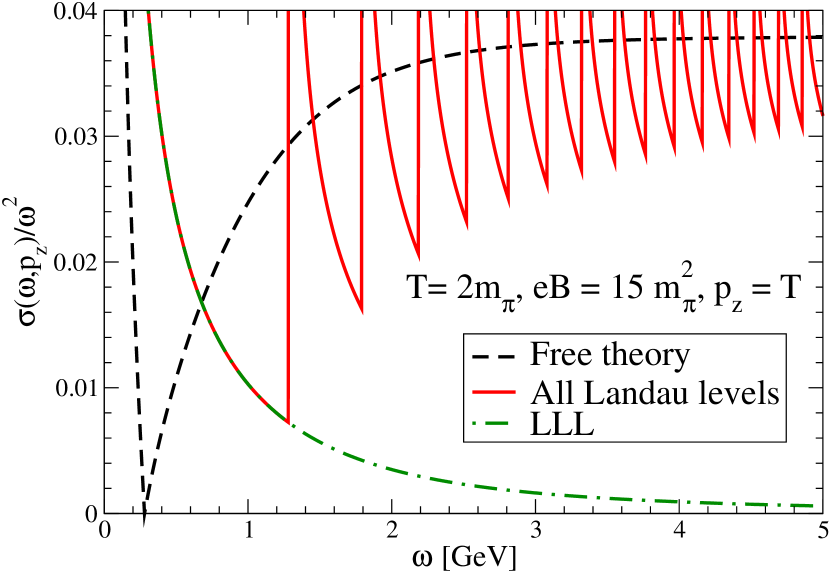
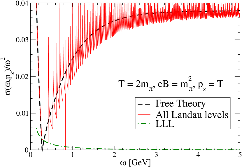
Figure 2: Spectral function in the pseudoscalar channel for two different values of field strength. The meson state is assumed to be made up of massless $u$ quarks.

In Fig. 2, we show spectral function in the limit $p_{\bot}=0$. The sawtooth nature of the spectral function is due to singularities at particle thresholds. Physically at the point of threshold the meson is unstable with respect decay into quark-antiquark pair. The origin of these singularities are dimensional reduction and infinitesimally narrow Landau levels which are artefact of lowest order of perturbation theory. Let us note that the peaks become narrower and the their number increases as the intensity of the magnetic field decreases. This is easy to understand. For a given $\omega$, the highest Landau level that contributes to the spectral function is $r_{\rm max}=\left\lfloor(s_{\parallel}-4m^{2})/(8\left\lvert q_{f}\mathcal{B}\right\rvert)\right\rfloor$ which increases with dwindling magnetic field. On the other hand, in the high frequency tail of the spectral function, the spacing between two successive peaks are given by $\delta\omega\simeq\left\lvert q_{f}\mathcal{B}\right\rvert/4\omega$ $(\omega\gg\left\lvert q_{f}\mathcal{B}\right\rvert)$, which decreases when magnetic field decreases or frequency increases.

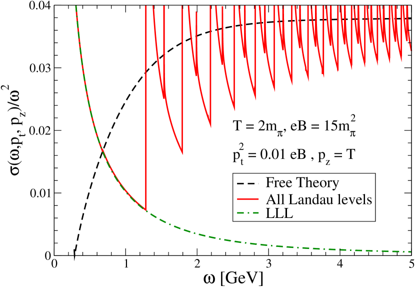
Figure 3: Same as Fig. 2 but for nonzero $p_{\bot}$ and only annihilation contribution is shown in the magnetized case. For $p_{\bot}\to 0$ we should get back Fig. 2. This is shown in the Right panel.

We show in Fig. 3 the spectral function for nonzero transverse momentum. The results are similar in nature to Fig. 2 but more spiky and stay above than the corresponding result at $p_{\bot}=0$. These can be understood as a consequence of availability of more decay channels at nonzero $p_{\bot}$.

3 Screening masses

At zero momenta, the spectral function is obtained from

$$\sigma\left(\omega\right)=N_{c}\sum_{l}\left(2-\delta_{l0}\right)\frac{\left\lvert q_{f}\mathcal{B}\right\rvert}{4\pi^{2}}\theta\left(\omega^{2}-8l\left\lvert q_{f}\mathcal{B}\right\rvert\right)\frac{\omega}{\sqrt{\omega^{2}-8l\left\lvert q_{f}\mathcal{B}\right\rvert}}\tanh{\frac{\beta\omega}{4}}$$ (23)

We notice that far away from the threshold, the spectral function for each mode consist of a frequency independent part together with power suppressed corrections. This is a consequence of dimensional reduction and is in contrast to the free field limit where spectral function grow as $\omega^{2}$.

Now, from (3) and (23), the temporal correlation function can be written as

$$\chi^{\tau}=\chi_{0}^{\tau}+\sum_{l>0}\chi_{l}^{\tau}\,,$$ (24)

where $\chi_{0}^{\tau}$ is the correlator with LLL approximation. $\chi_{0}^{\tau}$ is obtained as,

$$\tilde{\chi}_{0}^{\tau}=N_{c}\frac{\left\lvert q_{f}\mathcal{B}\right\rvert}{2\pi^{2}T^{2}}\left(1-2\tilde{\tau}\right)\frac{\pi}{\sin{\left(2\pi\tilde{\tau}\right)}}\,,$$ (25)

where $\tilde{\tau}=\tau/\beta$ and $\tilde{\chi}^{\tau}=\beta^{3}\chi^{\tau}$.

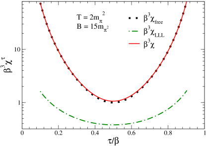
Figure 4: pseudoscalar correlator made up of up quark in presence of a magnetic field.

We show the temporal correlator in the presence of a magnetic field in Fig. 4. The effect of the magnetic field on the spectral function is marginal even for extreme value of the field achievable in the heavy ion collision. Let us also note that the contribution of LLL on the temporal correlator is small and an all order summation over the Landau levels is necessary. The screening mass in the time direction, on the other hand, is dictated by LLL. The screening mass is given by $m_{\rm scr}^{\tau}=2\pi T$ which is same as in free field theory. This behavior is understood as a consequence of $\mathcal{B}$ independence of LLL.

Now the immunity of $\chi^{\tau}$ to the exposure of $\mathcal{B}$ field can be understood in the following way. Using Euler-Mclaurin kind of relation between the sum of series and the integral of a function arfken_weber_2005 , it is not difficult to show that

$$\chi^{\tau}_{free}-\chi^{\tau}_{0}\leq\chi^{\tau}\leq\chi^{\tau}_{free}+\chi^{\tau}_{0}\,$$ (26)

where $\chi_{free}$ is the correlator in absence of magnetic field Florkowski:1993bq ,

$$\tilde{\chi}_{free}^{\tau}=\beta^{3}\chi_{free}^{\tau} = \frac{N_{C}}{\pi^{2}}\partial_{\tilde{\tau}^{2}}\left[\left(1-2\tilde{\tau}\right)\frac{\pi}{\sin{\left(2\pi\tilde{\tau}\right)}}\right]$$ (27)

$$= 2N_{c}\frac{\cos{\left(2\pi\tilde{\tau}\right)}}{\sin^{2}\left(2\pi\tilde{\tau}\right)}+N_{c}\pi\left(1-2\tilde{\tau}\right)\frac{\left(1+\cos^{2}\left(2\pi\tilde{\tau}\right)\right)}{\sin^{3}\left(2\pi\tilde{\tau}\right)}\,.$$

We have checked that inequality (26) is satisfied in our case. Thus change in the spectral function $\delta\chi=\chi-\chi_{free}\simeq\chi_{0}$ and this is small. Let us note that the derivation of (26) rests on the assumption that the correlator can be written as a sum over Landau levels and that it is a smooth function of the quantum number of orbital motion taken as a continuous variable. These are not overly restrictive assumptions and relations similar to (26) presumably hold in general.

The transverse plane correlator in LLL can written from (5) and (22) as

$$\chi^{xy}\left(\vec{x}_{\bot}\right)=N_{c}\frac{\left\lvert q_{f}\mathcal{B}\right\rvert}{4\pi^{2}}\int_{0}^{\infty}\,\frac{d\omega}{\omega}\tan{\left(\frac{\beta\omega}{4}\right)}\int\,\frac{d^{2}p_{\bot}}{\left(2\pi\right)^{2}}\,e^{i\vec{p}_{\bot}\cdot\vec{x}_{\bot}}\,e^{-\frac{p^{2}_{\bot}}{2\left\lvert q_{f}\mathcal{B}\right\rvert}}$$ (28)

The integration over transverse coordinates is a Gaussian one. The frequency integration is logarithmically divergent and hence needs regularization. Explicit from of regularization is not important at this point, it just yields a constant, say $A$. Now the correlator can be written as,

$$\chi^{xy}\left(\vec{x}_{\bot}\right)=AN_{c}\frac{\left\lvert q_{f}\mathcal{B}\right\rvert^{2}}{8\pi^{3}}\exp\left({-\frac{1}{2}\left\lvert q_{f}\mathcal{B}\right\rvert x^{2}_{\bot}}\right)$$ (29)

The correlator decays in the transverse direction with a characteristic range $\sqrt{\left\lvert q_{f}\mathcal{B}\right\rvert}$. But as alluded, this Gaussian falloff is not characteristics of typical screening behavior but rather a manifestation of magnetic confinement.

Using the following identity

$$n_{f}\left(x\right)=\frac{1}{2}-2\sum_{l=1}^{\infty}\frac{x}{\left(2l-1\right)^{2}\pi^{2}+x^{2}}\,$$ (30)

we obtain the longitudinal correlator from (5) and (22) as ,

$$\chi^{z}\left(z\right)=N_{c}\frac{\left\lvert q_{f}\mathcal{B}\right\rvert}{4\pi\beta}\sum_{l=1}^{\infty}\exp{\left(-2\pi\frac{\left(2l-1\right)\lvert z\rvert}{\beta}\right)}\,.$$ (31)

At large distance $l=1$ contribution dominates in (31). Thus longitudinal screening mass $m_{\rm scr}^{z}$ is $2\pi T$ which coincides with $m_{\rm scr}^{\tau}$. Let us note, however, that the asymptotic behavior of the correlator is different from free theory.

4 Outlook

We have derived analytic expression for spectral function in pseudoscalar (scalar) channel in the deconfined and magnetized phase of QCD and found spatial and temporal screening masses. While the results presented herein are nontrivial as no approximation has been made regarding the kinematics or strength of the magnetic field, it would be of import to include QCD corrections for any kind of realistic phenomenology. The point is that quarks interact strongly with the gluons. The strong interaction of quarks will inevitably mix the Landau levels and fuzz the distinction between $\parallel$ and $\perp$ spaces.

From the perspective of heavy ion collision phenomenology, we belive that it would more interesting to analyze the observables in a general background of electromagnetic field which is inhomogeneous and time dependent. These are work in progress and will be reported elsewhere.

Appendix A Imaginary part of one loop self energy

The integration over $k_{z}$ can easily be done with the help of the well known relation,

$$\delta\left(f\left(x\right)\right)=\sum_{i}\frac{\delta\left(x-x_{i}\right)}{\left\lvert\frac{\partial f\left(x\right)}{\partial x}\right\rvert_{x_{i}}}\,.$$ (32)

$x_{i}$ is simple zero of $f\left(x\right)$, $f\left(x_{i}\right)=0$. The imaginary part of $\mathcal{I}_{r,s}$ is given by,

$$\Im\left(\frac{\mathcal{I}_{r,s}}{\pi}\right) = -\frac{1}{8\pi}\int\frac{dk_{z}}{\omega_{r}\left(k\right)\omega_{s}\left(q\right)}\biggl{[}\biggl{(}1-n_{f}\left(\omega_{r}\left(k\right)\right)-n_{f}\left(\omega_{s}\left(q\right)\right)\biggr{)}\biggr{\{}\delta\left(\omega-\omega_{r}\left(k\right)-\omega_{s}\left(q\right)\right)$$ (33)

$$- \delta\left(\omega+\omega_{r}\left(k\right)+\omega_{s}\left(q\right)\right)\biggr{\}}+\biggl{(}n_{f}\left(\omega_{r}\left(k\right)\right)-n_{f}\left(\omega_{s}\left(q\right)\right)\biggr{)}\biggl{\{}\delta\left(\omega-\omega_{r}\left(k\right)+\omega_{s}\left(q\right)\right)$$

$$- \delta\left(\omega+\omega_{r}\left(k\right)-\omega_{s}\left(q\right)\right)\biggr{\}}\biggr{]}$$

where, $\omega_{r}\left(k\right)=\sqrt{k_{z}^{2}+\epsilon_{r}^{2}}$ and $\omega_{s}\left(q\right)=\sqrt{q_{z}^{2}+\epsilon_{s}^{2}}$. $\epsilon_{r}$ is transverse mass in $r$th Landau level, $\epsilon_{r}^{2}=m^{2}+2r\left\lvert q_{f}\mathcal{B}\right\rvert$. Let us introduce, $\chi_{r,s}=\frac{1}{2}\left(1+\frac{\epsilon_{r}^{2}-\epsilon_{s}^{2}}{s_{\parallel}}\right)$, $\lambda_{rs}=\lambda_{sr}=\frac{1}{2}\Lambda^{1/2}\left(1,\frac{\epsilon_{r}^{2}}{s_{\parallel}},\frac{\epsilon_{s}^{2}}{s_{\parallel}}\right)$ where, $\Lambda\left(x,y,z\right)=x^{2}+y^{2}+z^{2}-2xy-2yz-2zx$ is the triangle function. We also take $\omega_{rs}^{\pm}=\chi_{rs}\omega\pm\lambda_{rs}p_{z}$, $\tilde{\omega}_{rs}^{\pm}=\chi_{rs}\omega\pm\lambda_{rs}\lvert p_{z}\rvert$. The imaginary part can be written as,

$$\Im\left(\frac{\mathcal{I}_{r,s}}{\pi}\right) = -\theta\left(s_{\parallel}-\left(\epsilon_{r}+\epsilon_{s}\right)^{2}\right)\frac{1}{8\pi s_{\parallel}\lambda_{rs}}\biggl{(}2-n_{f}\left(\omega_{rs}^{+}\right)-n_{f}\left(\omega_{rs}^{-}\right)-n_{f}\left(\omega_{sr}^{+}\right)-n_{f}\left(\omega_{sr}^{-}\right)\biggr{)}$$ (34)

$$+ \biggl{(}\theta\left(s_{\parallel}\right)-\theta\left(s_{\parallel}-\left(\epsilon_{r}-\epsilon_{s}\right)^{2}\right)\biggr{)}\frac{1}{4\pi s_{\parallel}\lambda_{rs}}\biggl{(}2-n_{f}\left(\omega_{rs}^{+}\right)-n_{f}\left(\omega_{rs}^{-}\right)-n_{f}\left(\omega_{sr}^{+}\right)-n_{f}\left(\omega_{sr}^{-}\right)\biggr{)}$$

$$- \theta^{\star}\left(\epsilon_{r}-\epsilon_{s}\right)\theta\left(-s_{\parallel}\right)\frac{1}{8\pi s_{\parallel}\lambda_{rs}}\biggl{(}n_{f}\left(\tilde{\omega}_{rs}^{+}\right)-n_{f}\left(-\tilde{\omega}_{sr}^{-}\right)\biggr{)}$$

$$- \theta^{\star}\left(\epsilon_{s}-\epsilon_{r}\right)\theta\left(-s_{\parallel}\right)\frac{1}{8\pi s_{\parallel}\lambda_{rs}}\biggl{(}n_{f}\left(\tilde{\omega}_{sr}^{+}\right)-n_{f}\left(-\tilde{\omega}_{rs}^{-}\right)\biggr{)}$$

$$- \delta_{\epsilon_{r},\epsilon_{s}}\,\theta\left(-s_{\parallel}\right)\frac{1}{4\pi s_{\parallel}\lambda_{rs}}\biggl{(}n_{f}\left(\tilde{\omega}_{rr}^{+}\right)-n_{f}\left(-\tilde{\omega}_{rr}^{-}\right)\biggr{)}\,,$$

where $\theta*\left(x\right)$ is Heaviside theta function with the condition that $\theta^{*}\left(0\right)=0$.

Appendix B Evaluation of $\mathcal{T}$ intergrals

The $\mathcal{T}$ integrals in the main text have following structure,

$$\mathcal{T}_{m,n}^{\alpha,\beta,\gamma}=\left(-1\right)^{m+n}\int\frac{d^{2}k_{\perp}}{\left(2\pi\right)^{2}}e^{-\left(\rho_{k}+\rho_{q}\right)}L_{m}^{\alpha}\left(2\rho_{k}\right)L_{n}^{\beta}\left(2\rho_{q}\right)\left(\vec{k}\cdot\vec{q}\right)^{\gamma}\,.$$ (35)

Let us scale momentum variables as $x=\frac{2k_{\perp}^{2}}{|q_{f}B|}$ and $\xi=\frac{2p_{\perp}^{2}}{|q_{f}B|}$ in (35). We can write

$$\mathcal{T}_{m,n}^{\alpha,\beta,\gamma}=\left(-1\right)^{m+n}\frac{\lvert q_{f}\mathcal{B}\rvert}{16\pi^{2}}\left(\frac{\lvert q_{f}\mathcal{B}\rvert}{2}\right)^{\gamma}e^{-\frac{\xi}{2}}\mathcal{\chi}^{\alpha,\beta,\gamma}_{m,n}\,,$$ (36)

where

$$\mathcal{\chi}^{\alpha,\beta,\gamma}_{m,n}=\int_{0}^{\infty}dx\int_{0}^{2\pi}d\phi\,e^{-\left(x-\sqrt{x\xi}\cos{\phi}\right)}L_{m}^{\alpha}\left(x\right)L_{n}^{\beta}\left(x+\xi-2\sqrt{x\xi}\cos{\phi}\right)\left(x-\sqrt{x\xi}\cos{\phi}\right)^{\gamma}\,.$$ (37)

(37) is defined for arbitrary positive values of $\alpha$, $\beta$ or $\gamma$. For our purpose, we need to evaluate a small subset of this where $\alpha=\beta=\gamma\in\left\{0,1\right\}$. When $\xi=0$, $\mathcal{\chi}_{m,n}^{\alpha}=\mathcal{\chi}_{m,n}^{\alpha,\alpha,\alpha}$ express the orthogonality relation for Laguerre polynomials,

$$\mathcal{\chi}^{\alpha,\alpha,\alpha}_{m,n}=2\pi\frac{\Gamma\left(\alpha+n+1\right)}{\Gamma\left(n+1\right)}\delta_{m,n}\,.$$ (38)

For nonzero value of $\xi$ deterministic numerical integrators perform fairly well to evaluate diagonal elements $\mathcal{\chi}_{mm}^{\alpha}$ for moderate value of $\xi$. For extreme values of $\xi$ or when $\lvert m-n\rvert$ is large, success of cubature routines are uncertain due to oscillatory nature of the integrand in (37). We can, however, circumvent this problem by expanding $\mathcal{\chi}$ in a polynomial basis. Since $\mathcal{\chi}$ is an analytic function of $\xi$, such an expansion is always possible and it provides a fast, stable and accurate method for the numerical evaluation of (37). In addition to this, analytic expressions for $\mathcal{\chi}$ may prove to be useful to test the accuracy of the results obtained from approximate forms of propagators.

We assume a Laguerre-Fourier expansion of $\mathcal{\chi}$

$$\mathcal{\chi}\left(\xi\right)=\sum_{l=0}^{\infty}c_{l}^{\delta}L_{l}^{\delta}\left(\xi\right)\,,$$ (39)

and our task boils down to finding out the coefficients $c_{l}^{\delta}$ which we will do in a heuristic way.

Let us first consider $\mathcal{\chi}_{mn}^{0}$. The strategy here is to exponentiate the angular dependence in one of the Laguerre polynomial in (37) using a nice addition formula due to Bateman bateman1932partial ,

$$e^{\sqrt{x\xi}e^{i\phi}}L_{n}^{\beta}\left(x+\xi-2\sqrt{x\xi}\cos{\phi}\right)=\sum_{k=0}^{\infty}\left(\sqrt{x\xi}e^{i\phi}\right)^{k-n}\frac{n!}{k!}L_{n}^{k-n}\left(x\right)L_{n}^{k-n}\left(\xi\right)\,.$$ (40)

We multiply both sides of (40) by $e^{-i\sqrt{x\xi}\cos{\phi}}$ and substitute it in (37). The innermost angular integration can be performed using Sommerfeld’s representation of Bessel function,

$$J_{\nu}\left(u\right)=\frac{1}{2\pi}\int_{0}^{2\pi}d\phi\,e^{iu\sin{\phi}-i\nu\phi}\,,\quad\text{$\nu$ is an integer}.$$ (41)

The $x$ integration then can be done with the following identity kolbig1996hankel ,

$$\int_{0}^{\infty}\,dx\,e^{-x}\left(\sqrt{x}\right)^{\gamma+\lambda}J_{\gamma+\lambda}\left(b\sqrt{x}\right)L_{m}^{\gamma}\left(x\right)L_{n}^{\lambda}\left(x\right)$$

$$\,\,\,=\left(-1\right)^{m+n}\left(\frac{b}{2}\right)^{\gamma+\lambda}e^{-\frac{b^{2}}{4}}\,L_{m}^{\gamma+m-n}\left(\frac{b^{2}}{4}\right)L_{n}^{\lambda+n-m}\left(\frac{b^{2}}{4}\right)\,.$$ (42)

So we have,

$$\mathcal{\chi}^{0}_{m,n} = \left(-1\right)^{m+n}2\pi\Gamma\left(n+1\right)\left(\frac{\xi}{2}\right)^{-n}e^{-\frac{\xi}{4}}L_{n}^{m-n}\left(\frac{\xi}{4}\right)$$ (43)

$$\times \sum_{k=0}^{n}\frac{1}{k!}\left(\frac{\xi}{2}\right)^{k}L_{n}^{k-n}\left(\xi\right)L_{m}^{m-n}\left(\frac{\xi}{4}\right)\,.$$

We can further simplify (43) by using the following identity erdelyi1940transformation ,

$$\sum_{k=0}^{\infty}L_{m}^{\left(k+\alpha\right)}\left(x\right)L_{n}^{\left(k+\beta\right)}\left(y\right)\frac{z^{k}}{k!}=e^{z}\sum_{k=0}^{\text{min}(m,n)}L_{m-k}^{\left(k+\alpha\right)}\left(x-z\right)L_{n-k}^{\left(k+\beta\right)}\left(y-z\right)\frac{z^{k}}{k!}\,,$$ (44)

together with the fact that $L_{\nu}^{-\nu}\left(x\right)=(-x)^{\nu}/\nu!$. The upshot is an amazingly simple expression for $\mathcal{\chi}^{0}_{m,n}$,

$$\mathcal{\chi}^{0}_{m,n}=\left(-1\right)^{m}\frac{2\pi e^{\frac{\xi}{4}}}{\Gamma\left(m+1\right)}U\left(-m,-m+n+1,\frac{\xi}{4}\right)L_{n}^{m-n}\left(\frac{\xi}{4}\right)\,,$$ (45)

where $U(a,b,z)$ is Tricomi’s confluent hypergeometric function.

The expression for $\mathcal{\chi}_{m,n}^{1}$ is somewhat complicated. To evaluate it, we start with the following generalization of (40)koornwinder1977addition ,

$$e^{\sqrt{x\xi}e^{i\phi}}L_{n}^{\beta}\left(x+\xi-2\sqrt{x\xi}\cos{\phi}\right)=\sum_{k=0}^{\infty}\sum_{s=0}^{n}\mathcal{C}^{\beta}_{nks}\left(\sqrt{x\xi}\right)^{k+s}L_{n-s}^{\beta+k+s}\left(x\right)L_{n-s}^{\beta+k+s}\left(\xi\right)e^{i\phi\left(k-s\right)}\,,$$ (46)

where

$$\mathcal{C}^{\beta}_{nks}=\frac{\left(\beta+k+s\right)\Gamma\left(\beta+s\right)\Gamma\left(\beta+k\right)\Gamma\left(n-s+1\right)}{\Gamma\left(\beta\right)\Gamma\left(s+1\right)\Gamma\left(k+1\right)\Gamma\left(\beta+n+k+1\right)}\,,\beta\neq 0.$$ (47)

As in the earlier case, (46) allows to perform the angular integration. The $x$ integration is likewise recast in the form of a Hankel transform, a convenient closed form expression for which can be derived as,

$$\mathcal{H}_{m,n}^{\mu,\nu,\alpha,\beta} = \int_{0}^{\infty}\,dx\,e^{-x}x^{\mu+\frac{\nu}{2}}L_{m}^{\alpha}\left(x\right)L_{n}^{\beta}\left(x\right)J_{\nu}\left(\sqrt{x\xi}\right)$$ (48)

$$= \left(-1\right)^{m+n}\Gamma\left(\mu+1\right)\left(\frac{\sqrt{\xi}}{2}\right)^{\nu}e^{-\frac{\xi}{4}}\sum_{r=0}^{\mu}\sum_{l=0}^{\gamma}\frac{\left(-1\right)^{r}}{r!}\binom{\mu+\nu}{\mu-r}\binom{\gamma}{l}$$

$$\times L_{n}^{\alpha+m+l-n}\left(\frac{\xi}{4}\right)L_{m+l-\gamma}^{\beta+n+\gamma-l-m}\left(\frac{\xi}{4}\right)\,,$$

where $\gamma=\mu+\nu-\alpha-\beta+r$ and $\mu+\nu>-1$. For $\gamma<0$, the uppper limit of $l$ summation in (48) has to be replaced by $\infty$. For $\mu=0,\nu=\alpha+\beta$ (48) reduces to (42).

After a short algenbra $\mathcal{\chi}^{1}_{m,n}$ can be expressed as,

$$\mathcal{\chi}^{1}_{m,n} = {{}^{a}\mathcal{\chi}}^{1}_{m,n}-{{}^{b}\mathcal{\chi}}^{1}_{m,n}\,,$$

$${{}^{a}\mathcal{\chi}}^{1}_{m,n} = 2\pi\sum_{k=0}^{\infty}\sum_{s=0}^{n}\mathcal{C}^{\beta}_{nks}\left(\sqrt{\xi}^{k+s}\right)\mathcal{H}_{m,n-s}^{s+1,k-s,1,k+s+1}\,,$$

$${{}^{b}\mathcal{\chi}}^{1}_{m,n} = 2\pi\sum_{k=0}^{\infty}\sum_{s=0}^{n}\mathcal{C}^{\beta}_{nks}\left(\sqrt{\xi}^{k+s}\right)\left(k-s\right)\mathcal{H}_{m,n-s}^{s,k-s,1,k+s+1}\,.$$ (49)

References

- (1) Y. Aoki, G. Endrodi, Z. Fodor, S. D. Katz and K. K. Szabo, The Order of the quantum chromodynamics transition predicted by the standard model of particle physics, Nature 443 (2006) 675–678, [hep-lat/0611014].
- (2) D. E. Kharzeev, L. D. McLerran and H. J. Warringa, The Effects of topological charge change in heavy ion collisions: ‘Event by event P and CP violation’, Nucl. Phys. A803 (2008) 227–253, [0711.0950].
- (3) V. Skokov, A. Yu. Illarionov and V. Toneev, Estimate of the magnetic field strength in heavy-ion collisions, Int. J. Mod. Phys. A24 (2009) 5925–5932, [0907.1396].
- (4) A. Bzdak and V. Skokov, Event-by-event fluctuations of magnetic and electric fields in heavy ion collisions, Phys. Lett. B710 (2012) 171–174, [1111.1949].
- (5) V. Voronyuk, V. D. Toneev, W. Cassing, E. L. Bratkovskaya, V. P. Konchakovski and S. A. Voloshin, (Electro-)Magnetic field evolution in relativistic heavy-ion collisions, Phys. Rev. C83 (2011) 054911, [1103.4239].
- (6) W.-T. Deng and X.-G. Huang, Event-by-event generation of electromagnetic fields in heavy-ion collisions, Phys. Rev. C85 (2012) 044907, [1201.5108].
- (7) D. Kharzeev, Parity violation in hot QCD: Why it can happen, and how to look for it, Phys. Lett. B633 (2006) 260–264, [hep-ph/0406125].
- (8) P. V. Buividovich, M. N. Chernodub, E. V. Luschevskaya and M. I. Polikarpov, Numerical evidence of chiral magnetic effect in lattice gauge theory, Phys. Rev. D80 (2009) 054503, [0907.0494].
- (9) K. Fukushima, D. E. Kharzeev and H. J. Warringa, Real-time dynamics of the Chiral Magnetic Effect, Phys. Rev. Lett. 104 (2010) 212001, [1002.2495].
- (10) G. S. Bali, F. Bruckmann, G. Endrodi, Z. Fodor, S. D. Katz, S. Krieg et al., The QCD phase diagram for external magnetic fields, JHEP 02 (2012) 044, [1111.4956].
- (11) G. S. Bali, F. Bruckmann, G. Endrodi, Z. Fodor, S. D. Katz and A. Schafer, QCD quark condensate in external magnetic fields, Phys. Rev. D86 (2012) 071502, [1206.4205].
- (12) E. S. Fraga and L. F. Palhares, Deconfinement in the presence of a strong magnetic background: an exercise within the MIT bag model, Phys. Rev. D86 (2012) 016008, [1201.5881].
- (13) D. Kharzeev et al., eds., Strongly Interacting Matter in Magnetic Fields. Springer., 2013.
- (14) A. K. Harding and D. Lai, Physics of Strongly Magnetized Neutron Stars, Rept. Prog. Phys. 69 (2006) 2631, [astro-ph/0606674].
- (15) T. Vachaspati, Magnetic fields from cosmological phase transitions, Phys. Lett. B265 (1991) 258–261.
- (16) H. Gies, J. Jaeckel and A. Ringwald, Polarized Light Propagating in a Magnetic Field as a Probe of Millicharged Fermions, Phys. Rev. Lett. 97 (2006) 140402, [hep-ph/0607118].
- (17) V. A. Miransky and I. A. Shovkovy, Quantum field theory in a magnetic field: From quantum chromodynamics to graphene and Dirac semimetals, Phys. Rept. 576 (2015) 1–209, [1503.00732].
- (18) E. V. Shuryak, Correlation functions in the QCD vacuum, Rev. Mod. Phys. 65 (1993) 1–46.
- (19) C. E. Detar and J. B. Kogut, The Hadronic Spectrum of the Quark Plasma, Phys. Rev. Lett. 59 (1987) 399.
- (20) C. E. Detar and J. B. Kogut, Measuring the Hadronic Spectrum of the Quark Plasma, Phys. Rev. D36 (1987) 2828.
- (21) W. Florkowski and B. L. Friman, Spatial dependence of the finite temperature meson correlation function, Z. Phys. A347 (1994) 271–276.
- (22) F. Karsch, M. G. Mustafa and M. H. Thoma, Finite temperature meson correlation functions in HTL approximation, Phys. Lett. B497 (2001) 249–258, [hep-ph/0007093].
- (23) W. M. Alberico, A. Beraudo, P. Czerski and A. Molinari, Finite momentum meson correlation functions in a QCD plasma, Nucl. Phys. A775 (2006) 188–211, [hep-ph/0605060].
- (24) M. Vepsalainen, Mesonic screening masses at high temperature and finite density, JHEP 03 (2007) 022, [hep-ph/0701250].
- (25) Y. Burnier and M. Laine, Massive vector current correlator in thermal QCD, JHEP 11 (2012) 086, [1210.1064].
- (26) F. Karsch, E. Laermann, P. Petreczky and S. Stickan, Infinite temperature limit of meson spectral functions calculated on the lattice, Phys. Rev. D68 (2003) 014504, [hep-lat/0303017].
- (27) G. Aarts and J. M. Martinez Resco, Continuum and lattice meson spectral functions at nonzero momentum and high temperature, Nucl. Phys. B726 (2005) 93–108, [hep-lat/0507004].
- (28) B. B. Brandt, A. Francis, H. B. Meyer and H. Wittig, Thermal Correlators in the channel of two-flavor QCD, JHEP 03 (2013) 100, [1212.4200].
- (29) M. Cheng et al., Meson screening masses from lattice QCD with two light and the strange quark, Eur. Phys. J. C71 (2011) 1564, [1010.1216].
- (30) N. Sadooghi and F. Taghinavaz, Dilepton production rate in a hot and magnetized quark-gluon plasma, Annals Phys. 376 (2017) 218–253, [1601.04887].
- (31) S. S. Avancini, R. L. S. Farias, M. Benghi Pinto, W. R. Tavares and V. S. Timóteo, pole mass calculation in a strong magnetic field and lattice constraints, Phys. Lett. B767 (2017) 247–252, [1606.05754].
- (32) P. V. Buividovich and M. I. Polikarpov, Quark mass dependence of the vacuum electric conductivity induced by the magnetic field in SU(2) lattice gluodynamics, Phys. Rev. D83 (2011) 094508, [1011.3001].
- (33) P. V. Buividovich, M. N. Chernodub, D. E. Kharzeev, T. Kalaydzhyan, E. V. Luschevskaya and M. I. Polikarpov, Magnetic-Field-Induced insulator-conductor transition in SU(2) quenched lattice gauge theory, Phys. Rev. Lett. 105 (2010) 132001, [1003.2180].
- (34) S. Ghosh, A. Mukherjee, M. Mandal, S. Sarkar and P. Roy, Thermal effects on meson properties in an arbitrary magnetic field, 1704.05319.
- (35) A. Bandyopadhyay and S. Mallik, Effect of magnetic field on dilepton production in a hot plasma, Phys. Rev. D95 (2017) 074019, [1704.01364].
- (36) A. Bandyopadhyay, C. A. Islam and M. G. Mustafa, Electromagnetic spectral properties and Debye screening of a strongly magnetized hot medium, Phys. Rev. D94 (2016) 114034, [1602.06769].
- (37) S. Ghosh, A. Mukherjee, M. Mandal, S. Sarkar and P. Roy, Spectral properties of meson in a magnetic field, Phys. Rev. D94 (2016) 094043, [1612.02966].
- (38) A. Mukherjee, S. Ghosh, M. Mandal, P. Roy and S. Sarkar, Mass modification of hot pions in a magnetized dense medium, Phys. Rev. D96 (2017) 016024, [1708.02385].
- (39) G. S. Bali, B. B. Brandt, G. Endrodi and B. Glaessle, Meson masses in electromagnetic fields with Wilson fermions, 1707.05600.
- (40) A. Kuznetsov and N. Mikheev, Electroweak processes in external electromagnetic fields. Springer, 2003.
- (41) T.-K. Chyi, C.-W. Hwang, W. F. Kao, G.-L. Lin, K.-W. Ng and J.-J. Tseng, The weak field expansion for processes in a homogeneous background magnetic field, Phys. Rev. D62 (2000) 105014, [hep-th/9912134].
- (42) C. S. Machado, S. I. Finazzo, R. D. Matheus and J. Noronha, Modification of the Meson Mass in a Magnetic Field from QCD Sum Rules, Phys. Rev. D89 (2014) 074027, [1307.1797].
- (43) S. Cho, K. Hattori, S. H. Lee, K. Morita and S. Ozaki, Charmonium Spectroscopy in Strong Magnetic Fields by QCD Sum Rules: S-Wave Ground States, Phys. Rev. D91 (2015) 045025, [1411.7675].
- (44) D. J. Broadhurst and S. C. Generalis, Can mass singularities be minimally subtracted?, Phys. Lett. 142B (1984) 75–79.
- (45) S. Zschocke, T. Hilger and B. Kampfer, In-medium operator product expansion for heavy-light-quark pseudoscalar mesons, Eur. Phys. J. A47 (2011) 151, [1112.2477].
- (46) A. G. Grozin, Methods of calculation of higher power corrections in QCD, Int. J. Mod. Phys. A10 (1995) 3497–3529, [hep-ph/9412238].
- (47) A. Patkos and N. Sakai, The Effect of the Nonperturbative Vacuum in Annihilation, Nucl. Phys. B168 (1980) 521–533.
- (48) A. Chodos, K. Everding and D. A. Owen, QED With a Chemical Potential: 1. The Case of a Constant Magnetic Field, Phys. Rev. D42 (1990) 2881–2892.
- (49) V. P. Gusynin, V. A. Miransky and I. A. Shovkovy, Dimensional reduction and catalysis of dynamical symmetry breaking by a magnetic field, Nucl. Phys. B462 (1996) 249–290, [hep-ph/9509320].
- (50) H. A. Weldon, Simple Rules for Discontinuities in Finite Temperature Field Theory, Phys. Rev. D28 (1983) 2007.
- (51) G. B. Arfken and H. J. Weber, Mathematical Methods for Physicists. Elsevier, 6 ed., 2005.
- (52) H. Bateman, Partial differential equations of mathematical physics. Cambridge University Press, Cambridge, England, 1932.
- (53) K. S. Kölbig and H. Scherb, On a hankel transform integral containing an exponential function and two laguerre polynomials, Journal of computational and applied mathematics 71 (1996) .
- (54) A. Erdélyi, Transformation of a certain series of products of confluent hypergeometric functions. applications to laguerre and charlier polynomials, Compositio Mathematica 7 (1940) 340–352.
- (55) T. Koornwinder, The addition formula for laguerre polynomials, SIAM Journal on Mathematical Analysis 8 (1977) .