Multiphase Flows of $N$ Immiscible Incompressible Fluids: An Outflow/Open Boundary Condition and Algorithm

Abstract

We present a set of effective outflow/open boundary conditions and an associated algorithm for simulating the dynamics of multiphase flows consisting of $N$ ($N\geqslant 2$) immiscible incompressible fluids in domains involving outflows or open boundaries. These boundary conditions are devised based on the properties of energy stability and reduction consistency. The energy stability property ensures that the contributions of these boundary conditions to the energy balance will not cause the total energy of the N-phase system to increase over time. Therefore, these open/outflow boundary conditions are very effective in overcoming the backflow instability in multiphase systems. The reduction consistency property ensures that if some fluid components are absent from the N-phase system then these N-phase boundary conditions will reduce to those corresponding boundary conditions for the equivalent smaller system. Our numerical algorithm for the proposed boundary conditions together with the N-phase governing equations involves only the solution of a set of de-coupled individual Helmholtz-type equations within each time step, and the resultant linear algebraic systems after discretization involve only constant and time-independent coefficient matrices which can be pre-computed. Therefore, the algorithm is computationally very efficient and attractive. We present extensive numerical experiments for flow problems involving multiple fluid components and inflow/outflow boundaries to test the proposed method. In particular, we compare in detail the simulation results of a three-phase capillary wave problem with Prosperetti’s exact physical solution and demonstrate that the method developed herein produces physically accurate results.

Keywords: Outflow boundary condition; open boundary condition; energy stability; reduction consistency; phase field; multiphase flow;

1 Introduction

In this work we focus on the dynamics and interactions of a system of $N$ ($N\geqslant 2$) immiscible incompressible fluids in an unbounded flow domain. In order to numerically simulate such problems it is necessary to truncate the domain to a finite size. Consequently, part of the boundary in the computational domain will be open, in the sense that the fluids can freely leave (or even enter) the domain through such boundaries, and appropriate boundary conditions will be required on the open (or outflow) portions of the domain boundary. We are particularly concerned with situations in which the multitude of fluid interfaces formed in the system will pass through the open domain boundaries. Following the notation of our previous works Dong2014 ; Dong2015 ; Dong2017 , we refer to such problems as N-phase outflows. Here $N$ denotes the number of different fluid components in the system, not necessarily the number of material phases.

N-phase outflows and open boundaries pose a number of issues to numerical simulations. First, the problem involves multiple fluid interfaces at the open/outflow boundary, which are associated with multiple surface tensions and the contrasts in densities and viscosities of these fluids. How to deal with the surface tensions, and the density and viscosity contrasts in the N-phase open/outflow boundary conditions (OBC) poses the foremost issue. Second, backflow instability is another crucial issue confronting N-phase outflow simulations. Backflow instability refers to the numerical instability associated with strong vortices or backflows at the open/outflow boundary, which causes computations to blow up instantly when strong vortices or backflows occur at the outflow boundary. The backflow instability issue is not unique to multiphase flows. This issue is well-known in single-phase outflow problems DongKC2014 ; DongS2015 ; Dong2015clesobc , but it becomes much worse for two-phase Dong2014obc ; DongW2016 and multiphase outflows because of the density contrasts and viscosity contrasts at the outflow boundary. Third, N-phase problems with $N\geqslant 3$ pose the so-called reduction consistency issue on the design of outflow/open boundary conditions Dong2017 . Reduction consistency refers to the property that, if only $M$ ($2\leqslant M\leqslant N-1$) fluid components are present in the N-phase system (while the other fluid components are absent), the governing equations and the boundary conditions for the N-phase system should reduce to those for the corresponding smaller M-phase system Dong2017 . The reduction consistency of N-phase outflow/open boundary conditions is an issue unique to multiphase outflow and open-boundary problems.

The development of effective outflow/open boundary conditions is an important problem in computational fluid dynamics. For single-phase problems, this has been under intensive investigations for decades and a large volume of literature exists; see e.g. Gresho1991 ; SaniG1994 for a comprehensive review of related literature and DongKC2014 ; Dong2015clesobc and the references therein for a sample of more recent works. On the other hand, for two-phase ($N=2$) outflows and open boundaries the existing work in the literature is very limited, and for multiphase outflow and open-boundary problems involving three or more ($N\geqslant 3$) fluid components, there is no existing work available in the literature to the best of our knowledge. The zero-flux (Neumann) and extrapolation boundary conditions from single-phase flows have been used for the two-phase Lattice-Boltzmann equation in LouGS2013 . The zero-flux condition has also been employed for the outflow boundary with a level-set type method in AlbadawiDRMD2013 ; Son2001 . The outflow condition for two immiscible fluids is considered for a porous medium in LenzingerS2010 , and for one-dimensional two-phase compressible flows in Munkejord2006 ; DesmaraisK2014 . In Dong2014obc ; DongW2016 we have developed a set of two-phase open boundary conditions having the attractive property that these conditions ensure the energy stability of the two-phase system, which is therefore effective for dealing with two-phase open boundaries.

In the current paper we consider the multiphase outflow and open-boundary problem with $N$ ($N\geqslant 3$) immiscible incompressible fluid components in the system, and present a set of effective outflow/open boundary conditions and an associated numerical algorithm for such problems within the phase field framework. The proposed open boundary conditions are designed based on considerations of two properties: energy stability and reduction consistency. By looking into the energy balance of the N-phase system, we design the open boundary conditions in such a way to ensure that their contributions shall not cause the total energy of the N-phase system to increase over time, regardless of the flow state at the outflow/open boundary. This energy-stable property holds even in situations where strong vortices or backflows occur at the open boundary. As a result, these boundary conditions are very effective in overcoming the backflow instability. We then look into the reduction consistency of these boundary conditions, and study how these conditions transform if some fluid components are absent from the N-phase system. The reduction consistency property limits the choice and the form of those boundary conditions that ensure the energy stability. The N-phase outflow/open boundary conditions and also the inflow boundary conditions proposed herein satisfy both the energy stability and the reduction consistency.

The outflow/open boundary conditions proposed herein are developed in the context of an N-phase physical formulation we developed recently in Dong2017 . This formulation is based on a phase field model for the N-fluid mixture that is more general than a previous model Dong2014 . The thermodynamic consistency and the reduction consistency of this formulation have been extensively studied in Dong2017 . The formulation rigorously satisfies the mass conservation, momentum conservation, the second law of thermodynamics, and the Galilean invariance principle. This formulation is fully reduction consistent, provided that an appropriate potential free energy density function satisfying certain properties is employed for the N-phase system Dong2017 . The reduction consistency of a set of Cahn-Hilliard type equations for a three-component and multi-component system (without hydrodynamic interactions) has previously been considered in BoyerL2006 ; BoyerM2014 . The thermodynamic consistency of two-phase and multiphase systems has also been considered in LowengrubT1998 ; KimL2005 ; AbelsGG2012 ; HeidaMR2012 ; Dong2014 ; LiW2014 ; Dong2015 ; WuX2017 . We refer the reader to e.g. AndersonMW1998 ; LiuS2003 ; YueFLS2004 ; BoyerLMPQ2010 ; Kim2012 ; ZhangW2016 ; BanasN2017 ; YangZWS2017 ; ZhaoLWY2017 for other contributions to two-phase and multiphase flow problems.

We further present an efficient numerical algorithm for the proposed outflow and inflow boundary conditions together with the N-phase governing equations. This is a semi-implicit splitting type scheme. Special care is taken in the numerical treatments of the open/ouflow boundary conditions such that the computations for different flow variables and the computations for the ($N-1$) phase field functions have all been de-coupled. The algorithm involves only the solution of a set of individual de-coupled Helmholtz-type equations (including Poisson) within each time step. The resultant linear algebraic systems after discretization involves only constant and time-independent coefficient matrices, which can be pre-computed during pre-processing, even when large density contrasts and large viscosity contrasts are involved in the N-phase system.

The novelties of this paper lie in two aspects: (i) the set of N-phase energy-stable and reduction-consistent outflow/open boundary conditions and inflow boundary conditions, and (ii) the numerical algorithm for treating the proposed set of outflow and inflow boundary conditions.

The rest of this paper is structured as follows. In the rest of this section we provide a summary of the general phase field model developed in Dong2017 for the N-fluid mixture. This model provides the basis for the N-phase energy balance relation and the development of energy-stable boundary conditions. In Section 2 we propose a set of outflow and inflow boundary conditions based on considerations of energy stability and reduction consistency of the N-phase system, and present an efficient algorithm for numerically treating these boundary conditions together with the N-phase governing equations. In Section 3 we present several representative numerical examples involving multiple fluid components and inflow/outflow boundaries to demonstrate the effectiveness of the proposed outflow/open boundary conditions and the performance of the numerical algorithm herein. Section 4 then concludes the discussion with some closing remarks.

1.1 A Thermodynamically Consistent N-Fluid Mixture Model

We summarize below the phase field model proposed in Dong2017 for an isothermal mixture of $N$ ($N\geqslant 2$) immiscible incompressible fluids. This model modifies and generalizes the N-phase model developed in Dong2014 , and it satisfies the conservations of mass and momentum, the second law of thermodynamics, and the Galilean invariance principle. This model forms the basis for the development of outflow/open boundary conditions in subsequent sections.

Consider a mixture of $N$ ($N\geqslant 2$) immiscible incompressible fluids contained in some flow domain $\Omega$ with boundary $\partial\Omega$. Let $\tilde{\rho}_{i}$ and $\tilde{\mu}_{i}$ ($1\leqslant i\leqslant N$) denote the constant densities and constant dynamic viscosities of these $N$ pure fluids (before mixing). Define auxiliary parameters

$$\tilde{\gamma}_{i}=\frac{1}{\tilde{\rho}_{i}},\ 1\leqslant i\leqslant N;\quad\Gamma=\sum_{i=1}^{N}\tilde{\gamma}_{i};\quad\Gamma_{\mu}=\sum_{i=1}^{N}\frac{\tilde{\mu}_{i}}{\tilde{\rho}_{i}}.$$ (1)

Let $\phi_{i}$ ($1\leqslant i\leqslant N-1$) denote the ($N-1$) independent order parameters, or interchangeably the phase field variables, that characterize the system, and $\vec{\phi}=(\phi_{1},\dots,\phi_{N-1})$. Let $\rho_{i}(\vec{\phi})$ and $c_{i}(\vec{\phi})$ ($1\leqslant i\leqslant N$) denote the density and volume fraction of fluid $i$ within the mixture, and let $\rho(\vec{\phi})$ denote the density of the N-phase mixture. Then we have the relations Dong2014

$$c_{i}=\frac{\rho_{i}}{\tilde{\rho}_{i}},\ 1\leqslant i\leqslant N;\quad\sum_{i=1}^{N}c_{i}=1;\quad\rho=\sum_{i=1}^{N}\rho_{i}.$$ (2)

Let $W(\vec{\phi},\nabla\vec{\phi})$ denote the free energy density function of the system which satisfies the condition, $\sum_{i=1}^{N-1}\nabla\phi_{i}\otimes\frac{\partial W}{\partial(\nabla\phi_{i})}=\sum_{i=1}^{N-1}\frac{\partial W}{\partial(\nabla\phi_{i})}\otimes\nabla\phi_{i},$ where $\otimes$ denote the tensor product. Then the motion of this N-phase system is described by the following equations Dong2017 :

$$\rho(\vec{\phi})\left(\frac{\partial\mathbf{u}}{\partial t}+\mathbf{u}\cdot\nabla\mathbf{u}\right)+\tilde{\mathbf{J}}\cdot\nabla\mathbf{u}=-\nabla p+\nabla\cdot\left[\mu(\vec{\phi})\mathbf{D}(\mathbf{u})\right]-\sum_{i=1}^{N-1}\nabla\cdot\left(\nabla\phi_{i}\otimes\frac{\partial W}{\partial(\nabla\phi_{i})}\right),$$ (3a)

$$\nabla\cdot\mathbf{u}=0,$$ (3b)

$$\sum_{j=1}^{N-1}\frac{\partial\varphi_{i}}{\partial\phi_{j}}\left(\frac{\partial\phi_{j}}{\partial t}+\mathbf{u}\cdot\nabla\phi_{j}\right)=\sum_{j=1}^{N-1}\nabla\cdot\left[\tilde{m}_{ij}(\vec{\phi})\nabla\mathcal{C}_{j}\right],\qquad 1\leqslant i\leqslant N-1,$$ (3c)

where $\mathbf{u}(\mathbf{x},t)$ is velocity, $p(\mathbf{x},t)$ is pressure, $\mathbf{D}(\mathbf{u})=\nabla\mathbf{u}+\nabla\mathbf{u}^{T}$ (superscript $T$ denoting transpose), $\mathbf{x}$ and $t$ are respectively the spatial and temporal coordinates. $\tilde{m}_{ij}$ ($1\leqslant i,j\leqslant N-1$) are coefficients and the matrix formed by these coefficients

$$\tilde{\mathbf{m}}=\begin{bmatrix}\tilde{m}_{ij}\end{bmatrix}_{(N-1)\times(N-1)}$$ (4)

is required to be symmetric positive definite (SPD) Dong2017 . $\varphi_{i}(\vec{\phi})$ are defined by

$$\varphi_{i}\equiv\rho_{i}(\vec{\phi})-\rho_{N}(\vec{\phi})=\varphi_{i}(\vec{\phi}),\quad 1\leqslant i\leqslant N-1.$$ (5)

The chemical potentials $\mathcal{C}_{i}(\vec{\phi},\nabla\vec{\phi})$ ($1\leqslant i\leqslant N-1$) are given by the following linear algebraic system

$$\sum_{j=1}^{N-1}\frac{\partial\varphi_{j}}{\partial\phi_{i}}\mathcal{C}_{j}=\frac{\partial W}{\partial\phi_{i}}-\nabla\cdot\frac{\partial W}{\partial(\nabla\phi_{i})},\quad 1\leqslant i\leqslant N-1,$$ (6)

which can be solved given $W(\vec{\phi},\nabla\vec{\phi})$ and $\varphi_{i}(\vec{\phi})$. $\tilde{\mathbf{J}}(\vec{\phi},\nabla\vec{\phi})$ takes the form

$$\tilde{\mathbf{J}}=-\sum_{i,j=1}^{N-1}\left(1-\frac{N}{\Gamma}\tilde{\gamma}_{i}\right)\tilde{m}_{ij}(\vec{\phi})\nabla\mathcal{C}_{j}.$$ (7)

The density of fluid $i$ within the mixture $\rho_{i}$, the volume fraction $c_{i}$, and the mixture density $\rho$ and dynamic viscosity $\mu$, are given by

$$\left\{\begin{split}&\rho_{i}(\vec{\phi})=\frac{1}{\Gamma}+\sum_{j=1}^{N-1}\left(\delta_{ij}-\frac{\tilde{\gamma}_{j}}{\Gamma}\right)\varphi_{j}(\vec{\phi}),\quad 1\leqslant i\leqslant N,\\ &c_{i}(\vec{\phi})=\tilde{\gamma}_{i}\rho_{i}(\vec{\phi})=\frac{\tilde{\gamma}_{i}}{\Gamma}+\sum_{j=1}^{N-1}\left(\tilde{\gamma}_{i}\delta_{ij}-\frac{\tilde{\gamma}_{i}\tilde{\gamma}_{j}}{\Gamma}\right)\varphi_{j}(\vec{\phi}),\quad 1\leqslant i\leqslant N,\\ &\rho(\vec{\phi})=\sum_{i=1}^{N}\rho_{i}=\frac{N}{\Gamma}+\sum_{i=1}^{N-1}\left(1-\frac{N}{\Gamma}\tilde{\gamma}_{i}\right)\varphi_{i}(\vec{\phi}),\\ &\mu(\vec{\phi})=\sum_{i=1}^{N}\tilde{\mu}_{i}c_{i}(\vec{\phi})=\frac{\Gamma_{\mu}}{\Gamma}+\sum_{i=1}^{N-1}\left(\tilde{\mu}_{i}-\frac{\Gamma_{\mu}}{\Gamma}\right)\tilde{\gamma}_{i}\varphi_{i}(\vec{\phi})\end{split}\right.$$ (8)

where $\delta_{ij}$ is the Kronecker delta.

In this model the functions $\varphi_{i}(\vec{\phi})$, the free energy density function $W(\vec{\phi},\nabla\vec{\phi})$, and the coefficients $\tilde{m}_{ij}$ ($1\leqslant i,k\leqslant N-1$) remain to be specified. Once they are known, all the other quantities can be computed. Note that the equation (5) is to define the set of order parameters $\vec{\phi}$. Once $\varphi_{i}(\vec{\phi})$ is given, the set of order parameters $\phi_{i}$ ($1\leqslant i\leqslant N-1$) will be fixed.

2 N-Phase Energy-Stable Open Boundary Conditions

In this section we propose a set of N-phase outflow/open (and also inflow) boundary conditions based on considerations of energy stability and reduction consistency, and develop an algorithm for numerically treating the proposed boundary conditions together with the N-phase governing equations.

2.1 N-phase Energy Balance and Energy-Stable Boundary Conditions

We first derive the energy balance relation for the N-phase model represented by (3a)–(3c), and then based on this relation look into possible forms for the boundary conditions to ensure the energy stability of the N-phase system.

It is straightforward to verify that the $\rho(\vec{\phi})$ given by (8) and $\tilde{\mathbf{J}}(\vec{\phi},\nabla\vec{\phi})$ given by (7) satisfy the following relation

$$\frac{\partial\rho}{\partial t}+\mathbf{u}\cdot\nabla\rho=-\nabla\cdot\tilde{\mathbf{J}}$$ (9)

where we have used equations (3c) and (5). Let $\mathbf{T}=-p\mathbf{I}+\mu\mathbf{D}(\mathbf{u})$ denote the stress tensor, where $\mathbf{I}$ is the identity tensor. Then equation (3a) can be written as

$$\rho\frac{D\mathbf{u}}{Dt}+\tilde{\mathbf{J}}\cdot\nabla\mathbf{u}=\nabla\cdot\mathbf{T}-\sum_{i=1}^{N-1}\nabla\cdot\left(\nabla\phi_{i}\otimes\frac{\partial W}{\partial(\nabla\phi_{i})}\right),$$ (10)

where $\frac{D}{Dt}=\frac{\partial}{\partial t}+\mathbf{u}\cdot\nabla$ denote the material derivative. Taking the $L^{2}$ inner product between equation (10) and $\mathbf{u}$ leads to

$$\begin{split}\frac{\partial}{\partial t}\int_{\Omega}\frac{1}{2}\rho|\mathbf{u}|^{2}=&-\int_{\Omega}\frac{\mu}{2}\|\mathbf{D}(\mathbf{u})\|^{2}-\int_{\Omega}\sum_{i=1}^{N-1}\left[\nabla\cdot\left(\nabla\phi_{i}\otimes\frac{\partial W}{\partial\nabla\phi_{i}}\right)\right]\cdot\mathbf{u}\\ &+\int_{\partial\Omega}\left[\mathbf{n}\cdot\mathbf{T}\cdot\mathbf{u}-\frac{1}{2}(\mathbf{n}\cdot\tilde{\mathbf{J}})|\mathbf{u}|^{2}-\frac{1}{2}\rho|\mathbf{u}|^{2}\mathbf{n}\cdot\mathbf{u}\right]\end{split}$$ (11)

where $\mathbf{n}$ is the outward-pointing unit vector normal to $\partial\Omega$, and we have used the divergence theorem, the equations (3b) and (9), and the following relations

$$\left\{\begin{split}&(\nabla\cdot\mathbf{T})\cdot\mathbf{u}=\nabla\cdot(\mathbf{T}\cdot\mathbf{u})-\mathbf{T}:(\nabla\mathbf{u})^{T}=\nabla\cdot(\mathbf{T}\cdot\mathbf{u})+p\nabla\cdot\mathbf{u}-\frac{\mu}{2}\|\mathbf{D}(\mathbf{u})\|^{2},\\ &\rho\frac{D\mathbf{u}}{Dt}\cdot\mathbf{u}=\frac{D}{Dt}\left(\frac{1}{2}\rho|\mathbf{u}|^{2}\right)-\frac{D\rho}{Dt}\left(\frac{1}{2}|\mathbf{u}|^{2}\right),\\ &\left(\tilde{\mathbf{J}}\cdot\nabla\mathbf{u}\right)\cdot\mathbf{u}=\nabla\cdot\left(\frac{1}{2}|\mathbf{u}|^{2}\tilde{\mathbf{J}}\right)-\nabla\cdot\tilde{\mathbf{J}}\left(\frac{1}{2}|\mathbf{u}|^{2}\right).\end{split}\right.$$ (12)

Take the $L^{2}$ inner product between equation (3c) and $\mathcal{C}_{i}$, sum over $i$ from $1$ to $(N-1)$, and we arrive at

$$\int_{\Omega}\sum_{j=1}^{N-1}\left(\frac{\partial W}{\partial\phi_{j}}-\nabla\cdot\frac{\partial W}{\partial\nabla\phi_{j}}\right)\frac{D\phi_{j}}{Dt}=-\int_{\Omega}\sum_{i,j=1}^{N-1}\tilde{m}_{ij}\nabla\mathcal{C}_{i}\cdot\nabla\mathcal{C}_{j}+\int_{\partial\Omega}\sum_{i,j=1}^{N-1}\tilde{m}_{ij}(\mathbf{n}\cdot\nabla\mathcal{C}_{j})\mathcal{C}_{i}$$ (13)

where we have used the integration by part, the divergence theorem, and the equation (6). By noting the relations

$$\left\{\begin{split}&\frac{\partial W}{\partial t}=\sum_{i=1}^{N-1}\frac{\partial W}{\partial\phi_{i}}\frac{\partial\phi_{i}}{\partial t}+\sum_{i=1}^{N-1}\frac{\partial W}{\partial\nabla\phi_{i}}\cdot\nabla\frac{\partial\phi_{i}}{\partial t}\\ &\nabla\cdot\frac{\partial W}{\partial\nabla\phi_{i}}\frac{\partial\phi_{i}}{\partial t}=\nabla\cdot\left(\frac{\partial W}{\partial\nabla\phi_{i}}\frac{\partial\phi_{i}}{\partial t}\right)-\frac{\partial W}{\partial\nabla\phi_{i}}\cdot\nabla\frac{\partial\phi_{i}}{\partial t},\end{split}\right.$$ (14)

equation (13) can be transformed into

$$\int_{\Omega}\frac{\partial W}{\partial t}+\int_{\Omega}\sum_{i=1}^{N-1}\left(\frac{\partial W}{\partial\phi_{i}}-\nabla\cdot\frac{\partial W}{\partial\nabla\phi_{i}}\right)\mathbf{u}\cdot\nabla\phi_{i}-\int_{\partial\Omega}\sum_{i=1}^{N-1}\mathbf{n}\cdot\frac{\partial W}{\partial\nabla\phi_{i}}\frac{\partial\phi_{i}}{\partial t}\\ =-\int_{\Omega}\sum_{i,j=1}^{N-1}\tilde{m}_{ij}\nabla\mathcal{C}_{i}\cdot\nabla\mathcal{C}_{j}+\int_{\partial\Omega}\sum_{i,j=1}^{N-1}\tilde{m}_{ij}(\mathbf{n}\cdot\nabla\mathcal{C}_{j})\mathcal{C}_{i}$$ (15)

where we have used the divergence theorem. With the help of the relations

$$\left\{\begin{split}&\nabla\cdot\left(\nabla\phi_{i}\otimes\frac{\partial W}{\partial\nabla\phi_{i}}\right)\cdot\mathbf{u}=\nabla\cdot\left(\frac{\partial W}{\partial\nabla\phi_{i}}\otimes\nabla\phi_{i}\right)\cdot\mathbf{u}=\nabla\cdot\frac{\partial W}{\partial\nabla\phi_{i}}(\mathbf{u}\cdot\nabla\phi_{i})+\frac{\partial W}{\partial\nabla\phi_{i}}\cdot\nabla\nabla\phi_{i}\cdot\mathbf{u}\\ &\mathbf{u}\cdot\nabla W=\sum_{i=1}^{N-1}\frac{\partial W}{\partial\phi_{i}}\mathbf{u}\cdot\nabla\phi_{i}+\sum_{i=1}^{N-1}\frac{\partial W}{\partial\nabla\phi_{i}}\cdot\nabla\nabla\phi_{i}\cdot\mathbf{u}\\ &\mathbf{u}\cdot\nabla W=\nabla\cdot(\mathbf{u}W)\end{split}\right.$$ (16)

we can further transform (15) into

$$\begin{split}\frac{\partial}{\partial t}\int_{\Omega}W=&-\int_{\Omega}\sum_{i,j=1}^{N-1}\tilde{m}_{ij}\nabla\mathcal{C}_{i}\cdot\nabla\mathcal{C}_{j}+\int_{\Omega}\sum_{i=1}^{N-1}\nabla\cdot\left(\nabla\phi_{i}\otimes\frac{\partial W}{\partial\nabla\phi_{i}}\right)\cdot\mathbf{u}\\ &+\int_{\partial\Omega}\sum_{i,j=1}^{N-1}\tilde{m}_{ij}(\mathbf{n}\cdot\nabla\mathcal{C}_{j})\mathcal{C}_{i}+\int_{\partial\Omega}\sum_{i=1}^{N-1}\mathbf{n}\cdot\frac{\partial W}{\partial\nabla\phi_{i}}\frac{\partial\phi_{i}}{\partial t}-\int_{\partial\Omega}W(\mathbf{n}\cdot\mathbf{u})\end{split}$$ (17)

where we have used the divergence theorem and equation (3b).

Summing up equations (11) and (17), we obtain the energy balance equation for the N-phase system described by (3a)–(3c):

$$\begin{split}\frac{\partial}{\partial t}\int_{\Omega}\left[\frac{1}{2}\rho|\mathbf{u}|^{2}+W\right]=&-\int_{\Omega}\frac{\mu}{2}\|\mathbf{D}(\mathbf{u})\|^{2}-\int_{\Omega}\sum_{i,j=1}^{N-1}\tilde{m}_{ij}\nabla\mathcal{C}_{i}\cdot\nabla\mathcal{C}_{j}\\ &+\int_{\partial\Omega}\underbrace{\left[\mathbf{n}\cdot\mathbf{T}\cdot\mathbf{u}-\frac{1}{2}(\mathbf{n}\cdot\tilde{\mathbf{J}})|\mathbf{u}|^{2}-\frac{1}{2}\rho|\mathbf{u}|^{2}\mathbf{n}\cdot\mathbf{u}-W\mathbf{n}\cdot\mathbf{u}\right]}_{\text{boundary term (I)}}\\ &+\int_{\partial\Omega}\underbrace{\sum_{i,j=1}^{N-1}\tilde{m}_{ij}(\mathbf{n}\cdot\nabla\mathcal{C}_{j})\mathcal{C}_{i}}_{\text{boundary term (II)}}+\int_{\partial\Omega}\underbrace{\sum_{i=1}^{N-1}\mathbf{n}\cdot\frac{\partial W}{\partial\nabla\phi_{i}}\frac{\partial\phi_{i}}{\partial t}}_{\text{boundary term (III)}}.\end{split}$$ (18)

Since the free energy form $W(\vec{\phi},\nabla\vec{\phi})$ and the order parameters $\phi_{i}$ ($1\leqslant i\leqslant N-1$) are unspecified, the above energy balance holds for any specific form of $W(\vec{\phi},\nabla\vec{\phi})$ and any specific choice of the order parameters.

In the above energy balance equation, the left hand side (LHS) is the time derivative of the total energy of the N-phase system. On the right hand side (RHS), the volume-integral terms are always dissipative by noting the symmetric positive definiteness of the matrix formed by $\tilde{m}_{ij}$ ($1\leqslant i,j\leqslant N-1$). The boundary-integral terms, on the other hand, can be positive or negative, depending on the boundary conditions.

We are interested in boundary conditions for the flow and phase field variables which ensure that the boundary-integral terms (I), (II) and (III) in the energy balance equation (18) are non-positive. In other words, the contributions of the boundary terms will be dissipative under these conditions. As such, the total energy of the system will not increase over time, and this ensures the energy stability of the N-phase system. We refer to such boundary conditions as energy-stable boundary conditions.

We look into the following choices that ensure the dissipativeness of the boundary term (I) in equation (18):

$$\mathbf{u}=0,\quad\text{on}\ \partial\Omega;$$ (19a)

$$\mathbf{n}\cdot\mathbf{T}-W\mathbf{n}-\frac{1}{2}(\mathbf{n}\cdot\tilde{\mathbf{J}})\mathbf{u}-\frac{1}{2}\rho|\mathbf{u}|^{2}\mathbf{n}=0,\quad\text{on}\ \partial\Omega;$$ (19b)

$$\mathbf{n}\cdot\mathbf{T}-W\mathbf{n}-\frac{1}{2}(\mathbf{n}\cdot\tilde{\mathbf{J}})\mathbf{u}\\ -\rho\left[\theta\frac{1}{2}(\mathbf{u}\cdot\mathbf{u})\mathbf{n}+(1-\theta)\frac{1}{2}(\mathbf{n}\cdot\mathbf{u})\mathbf{u}-C_{1}(\mathbf{n},\mathbf{u})\mathbf{u}+C_{2}(\mathbf{n},\mathbf{u})\mathbf{n}\right]\Theta_{0}(\mathbf{n},\mathbf{u})=0,\quad\text{on}\ \partial\Omega;$$ (19c)

where $\theta$ is a constant parameter satisfying $0\leqslant\theta\leqslant 1$, and $C_{1}(\mathbf{n},\mathbf{u})\geqslant 0$ and $C_{2}(\mathbf{n},\mathbf{u})\geqslant 0$ are two non-negative constants or functions. $\Theta_{0}(\mathbf{n},\mathbf{u})$ is a smoothed step function given in DongS2015 , expressed as follows,

$$\Theta_{0}(\mathbf{n},\mathbf{u})=\frac{1}{2}\left(1-\tanh\frac{\mathbf{n}\cdot\mathbf{u}}{U_{0}\delta}\right),\quad\lim_{\delta\rightarrow 0}\Theta_{0}(\mathbf{n},\mathbf{u})=\Theta_{s0}(\mathbf{n},\mathbf{u})=\left\{\begin{array}[]{ll}1,&\text{if}\ \mathbf{n}\cdot\mathbf{u}<0\\ 0,&\text{otherwise}\end{array}\right.$$ (20)

where $U_{0}$ is a velocity scale, and $\delta>0$ is a small positive parameter that controls the sharpness of the smoothed step function. As $\delta\rightarrow 0$, $\Theta_{0}$ approaches the step function $\Theta_{s0}$, taking unit value when $\mathbf{n}\cdot\mathbf{u}<0$ and zero otherwise. The boundary condition (19b) ensures the energy stability. But it prohibits the kinetic energy from being convected out of the domain in the presence of inflow/outflows, resulting in poor physical results. The form of the $\Theta_{0}$ term in condition (19c) is inspired by the boundary condition developed in DongS2015 for the single-phase incompressible Navier-Stokes equations; see also Dong2014obc ; DongW2016 for two-phase flows. The condition (19c) ensures the energy dissipation of the boundary term (I) as $\delta\rightarrow 0$, i.e. when $\delta$ is sufficiently small, because with this condition

$$\begin{split}\mathbf{n}\cdot\mathbf{T}\cdot\mathbf{u}-\frac{1}{2}(\mathbf{n}\cdot\tilde{\mathbf{J}})|\mathbf{u}|^{2}&-\frac{1}{2}\rho|\mathbf{u}|^{2}\mathbf{n}\cdot\mathbf{u}-W\mathbf{n}\cdot\mathbf{u}\\ &=\left\{\begin{array}[]{ll}-C_{1}\rho|\mathbf{u}|^{2}+C_{2}\rho\mathbf{n}\cdot\mathbf{u}\leqslant 0,&\text{where}\ \mathbf{n}\cdot\mathbf{u}<0,\\ -\frac{1}{2}\rho|\mathbf{u}|^{2}\mathbf{n}\cdot\mathbf{u}\leqslant 0,&\text{where}\ \mathbf{n}\cdot\mathbf{u}\geqslant 0,\end{array}\right.\quad\text{on}\ \partial\Omega,\ \text{as}\ \delta\rightarrow 0.\end{split}$$ (21)

We look into the following choices that ensure the energy dissipation of the boundary term (II) in equation (18):

$$\sum_{i=1}^{N-1}\tilde{m}_{ij}\mathcal{C}_{i}=0,\quad 1\leqslant j\leqslant N-1,\quad\text{on}\ \partial\Omega;$$ (22a)

$$\sum_{j=1}^{N-1}\tilde{m}_{ij}\mathbf{n}\cdot\nabla\mathcal{C}_{j}=0,\quad 1\leqslant i\leqslant N-1,\quad\text{on}\ \partial\Omega;$$ (22b)

$$\sum_{j=1}^{N-1}\tilde{m}_{ij}\mathbf{n}\cdot\nabla\mathcal{C}_{j}=-\sum_{j=1}^{N-1}d_{ij}\mathcal{C}_{j},\quad 1\leqslant i\leqslant N-1,\quad\text{on\ }\ \partial\Omega;$$ (22c)

In (22c) $d_{ij}$ ($1\leqslant i,j\leqslant N-1$) are chosen coefficients, and the $(N-1)\times(N-1)$ matrix formed by $d_{ij}$ is required to be symmetric semi-positive definite. Because the matrix $\tilde{\mathbf{m}}$ formed by $\tilde{m}_{ij}$ is SPD, the boundary conditions (22a) and (22b) are equilvalent to $\mathcal{C}_{i}=0$ and $\mathbf{n}\cdot\nabla\mathcal{C}_{i}=0$ ($1\leqslant i\leqslant N-1$) on $\partial\Omega$, respectively.

We look into the following choices to ensure the dissipativeness of the boundary term (III) in equation (18):

$$\frac{\partial\phi_{i}}{\partial t}=0,\quad 1\leqslant i\leqslant N-1,\quad\text{on}\ \partial\Omega;$$ (23a)

$$\mathbf{n}\cdot\frac{\partial W}{\partial\nabla\phi_{i}}=0,\quad 1\leqslant i\leqslant N-1,\quad\text{on}\ \partial\Omega;$$ (23b)

$$\mathbf{n}\cdot\frac{\partial W}{\partial\nabla\phi_{i}}=-\sum_{j=1}^{N-1}q_{ij}\frac{\partial\phi_{j}}{\partial t},\quad 1\leqslant i\leqslant N-1,\quad\text{on}\ \partial\Omega;$$ (23c)

In (23c) $q_{ij}$ ($1\leqslant i,j\leqslant N-1$) are chosen coefficients, and the matrix formed by $q_{ij}$ is required to be symmetric semi-positive definite.

The boundary conditions (19a)–(19c), (22a)–(22c), and (23a)–(23c) are favorable from the energy stability standpoint. Additionally, the boundary conditions should satisfy the reduction consistency property for the N-phase systems, as pointed out by Dong2017 . The reduction consistency consideration can place restrictions on the form of these boundary conditions. In the subsequent section we look into the implications of the reduction consistency property on these boundary conditions, and in particular we suggest conditions for the inflow and outflow boundaries taking account of both reduction consistency and energy stability.

2.2 Reduction Consistency and Inflow/Outflow Boundary Conditions

The reduction consistency of N-phase formulations has been investigated extensively in Dong2017 . Let us first define reduction consistency according to Dong2017 , and then apply this requirement to the energy-stable boundary conditions from the previous subsection. A physical entity (e.g. variable, equation, or condition) for the N-phase system is said to be reduction consistent if it has the following property: If only a set of $M$ ($2\leqslant M\leqslant N-1$) fluid components are present in the N-phase system, then the physical entity for the N-phase system reduces to that for the corresponding equivalent M-phase system.

We insist that the formulation for the N-phase system should honor the reduction consistency property, namely, the N-phase formulation should be reduction consistent. Issues of reduction consistency have been considered recently in Dong2017 for the N-phase governing equations (coupled system of momentum and phase-field equations); see also BoyerL2006 ; BoyerM2014 for an investigation of the consistency issues of a system of Cahn-Hilliard type equations (without hydrodynamic interaction). The consistency properties explored in Dong2017 can be summarized as the following three:

1. The N-phase free energy density function should be reduction consistent;

2. The N-phase governing equations should be reduction consistent;

3. The boundary conditions for the N-phase system should be reduction consistent.

The goal of this subsection is to investigate the implications of the consistency property ($\mathscr{C}$3) on the energy-stable boundary conditions from the previous subsection.

To make the presentation more concrete, hereafter we will specifically employ the volume fractions of the first ($N-1$) fluids as the set of order parameters, namely,

$$\phi_{i}\equiv c_{i},\ \phi_{i}\in[0,1],\quad 1\leqslant i\leqslant N-1;\quad\vec{\phi}=\vec{c}=(c_{1},c_{2},\dots,c_{N-1})^{T}.$$ (24)

Then with this choice, equation (5) is given by (see Dong2015 for details)

$$\varphi_{i}(\vec{c})=\sum_{j=1}^{N-1}a_{ij}c_{j}-\tilde{\rho}_{N},\ \ 1\leqslant i\leqslant N-1;\quad a_{ij}=\tilde{\rho}_{i}\delta_{ij}+\tilde{\rho}_{N},\ \ 1\leqslant i,j\leqslant N-1$$ (25)

where $\delta_{ij}$ is the Kronecker delta. Let $\mathbf{A}_{1}=[a_{ij}]_{(N-1)\times(N-1)}$. It is straightforward to verify that $\mathbf{A}_{1}$ is symmetric positive definite and thus non-singular. It should be noted that the boundary conditions and numerical algorithms presented below can be formulated similarly in terms of the class of general order parameters introduced in Dong2015 .

Following Dong2017 , we employ the following general form for the free energy density function

$$W(\vec{c},\nabla\vec{c})=\sum_{i,j=1}^{N-1}\frac{\lambda_{ij}}{2}\nabla c_{i}\cdot\nabla c_{j}+H(\vec{c})$$ (26)

where the constants $\lambda_{ij}$ ($1\leqslant i,j\leqslant N-1$) are referred to as the mixing energy density coefficients, and the matrix $\mathbf{A}=[\lambda_{ij}]_{(N-1)\times(N-1)}$ is required to be symmetric positive definite. $H(\vec{c})$ is referred to as the potential energy density function, and is to be specified later. In this work we assume that the coefficients $\tilde{m}_{ij}$ ($1\leqslant i,j\leqslant N-1$) in (3c) are constants.

The following are the conditions obtained in Dong2017 about $\lambda_{ij}$, $H(\vec{c})$, and $\tilde{m}_{ij}$ based on the reduction consistency properties ($\mathscr{C}$1) and ($\mathscr{C}$2):

1. $\lambda_{ij}$ are given by

   $$\lambda_{ij}=\frac{3}{\sqrt{2}}\eta(\sigma_{iN}+\sigma_{jN}-\sigma_{ij}),\quad 1\leqslant i,j\leqslant N-1$$ (27)

   where $\eta$ is the characteristic interfacial thickness, $\sigma_{ij}$ ($1\leqslant i\neq j\leqslant N$) is the surface tension between fluids $i$ and $j$, and $\sigma_{ii}=0$ ($1\leqslant i\leqslant N$).

2. $\tilde{m}_{ij}$ are given by

   $$[\tilde{m}_{ij}]_{(N-1)\times(N-1)}=\tilde{\mathbf{m}}=m_{0}\mathbf{A}_{1}\mathbf{A}^{-1}\mathbf{A}_{1}^{T}$$ (28)

   where the constant $m_{0}>0$ is the mobility coefficient, $\mathbf{A}_{1}$ is the matrix formed by $a_{ij}$ as given in (25), and $\mathbf{A}$ is the matrix formed by $\lambda_{ij}$.

3. $H(\vec{c})$ is reduction consistent.

4. If any one fluid $k$ ($1\leqslant k\leqslant N$) is absent from the N-phase system, i.e. $c_{k}\equiv 0$, then $H(\vec{c})$ is chosen such that

   $$\left\{\begin{split}&L_{k}^{(N)}=0\\ &L_{i}^{(N-1)}=L_{i}^{(N)},\quad 1\leqslant i\leqslant k-1,\\ &L_{i}^{(N-1)}=L_{i+1}^{(N)},\quad k\leqslant i\leqslant N-1,\end{split}\right.$$ (29)

   where $L_{i}^{(N)}$ ($1\leqslant i\leqslant N$) is defined by

   $$\left\{\begin{split}&L_{i}^{(N)}=\sum_{j=1}^{N-1}\zeta_{ij}^{(N)}\frac{\partial H^{(N)}}{\partial c_{j}^{(N)}},\quad 1\leqslant i\leqslant N-1,\quad\text{where}\ \left[\zeta_{ij}^{(N)}\right]_{(N-1)\times(N-1)}=\mathbf{A}^{-1};\\ &L_{N}^{(N)}=-\sum_{i=1}^{N-1}L_{i}^{(N)}.\end{split}\right.$$ (30)

   In the above equations the superscript $N$ in $(\cdot)^{(N)}$ accentuates the point that the variable is with respect to the N-phase system.

It is shown in Dong2017 that, with $\lambda_{ij}$ and $\tilde{m}_{ij}$ given by (27) and (28) respectively, and $H(\vec{c})$ satisfying (DC-3) and (DC-4), the N-phase governing equations represented by (3a)–(3c) and the free energy density function given by (26) satisfy the reduction consistency properties ($\mathscr{C}$1) and ($\mathscr{C}$2).

In subsequent discussions, whenever necessary, we will use the superscript notation $(\cdot)^{(N)}$ to signify that the variable is with respect to the N-phase system, but will drop the superscript where no confusion arises.

2.2.1 Reduction Consistency of Boundary Conditions

We employ the $\lambda_{ij}$ and $\tilde{m}_{ij}$ values given by (27) and (28), and assume that the potential energy density function $H(\vec{c})$ satisfies the conditions (DC-3) and (DC-4). Let us now look into the energy-stable boundary conditions from Section 2.1 in light of the reduction consistency requirement ($\mathscr{C}$3).

We insist that the boundary conditions (19a)–(19c), (22a)–(22c) and (23a)–(23c) should satisfy the consistency property ($\mathscr{C}$3). To ensure the reduction consistency between the N-phase and M-phase ($2\leqslant M\leqslant N-1$) systems, it suffices to consider only the reduction between N-phase and ($N-1$)-phase systems, i.e. if only one fluid component is absent from the system.

Consider first the conditions (19a)–(19c). The condition (19a) is evidently reduction consistent because no phase field variable is involved. The conditions (19b) and (19c) are reduction consistent because, as shown in Dong2017 , the variables $\rho(\vec{c})$ and $\mu(\vec{c})$ given by (8) are reduction consistent, and the $\tilde{\mathbf{J}}$ given by (7) is also reduction consistent under the condition (DC-4). Note also that the free energy density function $W(\vec{c},\nabla\vec{c})$ given by (26) satisfies the consistency property ($\mathscr{C}$1) under the condition (DC-3), as mentioned earlier.

We next consider the boundary conditions (22a)–(22c). Define

$$\vec{\mathcal{C}}=\left[\mathcal{C}_{i}\right]_{(N-1)\times 1},\ \ \frac{\partial H}{\partial\vec{c}}=\left[\frac{\partial H}{\partial c_{i}}\right]_{(N-1)\times 1},\ \ \mathbf{D}=\left[d_{ij}\right]_{(N-1)\times(N-1)}.$$ (31)

In light of the equations (25), (26) and (27), the chemical potentials $\mathcal{C}_{i}$ can be obtained from equation (6) in a matrix form,

$$\vec{\mathcal{C}}=\mathbf{A}_{1}^{-T}\left(\frac{\partial H}{\partial\vec{c}}-\mathbf{A}\nabla^{2}\vec{c}\right).$$ (32)

So boundary condition (22a) is transformed into

$$\left\{\begin{split}&-\nabla^{2}\vec{c}+\mathbf{A}^{-1}\frac{\partial H}{\partial\vec{c}}=0,\ \ \text{on}\ \partial\Omega,\ \text{or equivalently}\\ &-\nabla^{2}c_{i}+\sum_{j=1}^{N-1}\zeta_{ij}\frac{\partial H}{\partial c_{j}}=0,\ \ 1\leqslant i\leqslant N-1,\ \ \text{on}\ \partial\Omega\end{split}\right.$$ (33)

where we have used (28). Boundary conditions (22b) can be transformed into

$$\left\{\begin{split}&\mathbf{n}\cdot\nabla\left(-\nabla^{2}\vec{c}+\mathbf{A}^{-1}\frac{\partial H}{\partial\vec{c}}\right)=0,\ \ \text{on}\ \partial\Omega,\ \text{or equivalently}\\ &\mathbf{n}\cdot\nabla\left(-\nabla^{2}c_{i}+\sum_{j=1}^{N-1}\zeta_{ij}\frac{\partial H}{\partial c_{j}}\right)=0,\ \ 1\leqslant i\leqslant N-1,\ \ \text{on}\ \partial\Omega.\end{split}\right.$$ (34)

Equations (33) and (34) are reduction consistent under the condition (DC-4). It suffices to consider only (33). Suppose the fluid $k$ (for any $1\leqslant k\leqslant N$) is absent from the N-phase system, i.e. $c_{k}^{(N)}\equiv 0$. Let $\chi_{i}$ denote a variable from the set of variables $\{c_{i},\rho_{i},\tilde{\rho}_{i},\tilde{\mu}_{i},\tilde{\gamma}_{i}\}$, and the following correspondence relations hold between the N-phase system and the ($N-1$)-phase system without fluid $k$:

$$\chi_{i}^{(N-1)}=\left\{\begin{array}[]{ll}\chi_{i}^{(N)},&1\leqslant i<k\\ \chi_{i+1}^{(N)},&k\leqslant i\leqslant N-1.\end{array}\right.$$ (35)

Therefore, for $1\leqslant i=k\leqslant N-1$, the equation (33) becomes an identity,

$$-\nabla^{2}c_{k}^{(N)}+\sum_{j=1}^{N-1}\zeta_{kj}^{(N)}\frac{\partial H^{(N)}}{\partial c_{j}^{(N)}}=-\nabla^{2}c_{k}^{(N)}+L_{k}^{(N)}=0$$ (36)

in light of the equation (29) under the condition (DC-4). For $1\leqslant i\leqslant k-1$, the equation (33) becomes

$$\begin{split}0&=-\nabla^{2}c_{i}^{(N)}+\sum_{j=1}^{N-1}\zeta_{ij}^{(N)}\frac{\partial H^{(N)}}{\partial c_{j}^{(N)}}=-\nabla^{2}c_{i}^{(N)}+L_{i}^{(N)}=-\nabla^{2}c_{i}^{(N-1)}+L_{i}^{(N-1)}\\ &=-\nabla^{2}c_{i}^{(N-1)}+\sum_{j=1}^{N-2}\zeta_{ij}^{(N-1)}\frac{\partial H^{(N-1)}}{\partial c_{j}^{(N-1)}},\quad 1\leqslant i\leqslant k-1\end{split}$$ (37)

where we have used the correspondence relation (35) and the equation (29) under the condition (DC-4). Therefore,

$$-\nabla^{2}c_{i}^{(N)}+\sum_{j=1}^{N-1}\zeta_{ij}^{(N)}\frac{\partial H^{(N)}}{\partial c_{j}^{(N)}}=0\ \ \Longrightarrow\ \ -\nabla^{2}c_{i}^{(N-1)}+\sum_{j=1}^{N-2}\zeta_{ij}^{(N-1)}\frac{\partial H^{(N-1)}}{\partial c_{j}^{(N-1)}}=0,\quad 1\leqslant i\leqslant k-1.$$ (38)

For $k+1\leqslant i+1\leqslant N$, equation (33) becomes

$$\begin{split}0&=-\nabla^{2}c_{i+1}^{(N)}+\sum_{j=1}^{N-1}\zeta_{i+1,j}^{(N)}\frac{\partial H^{(N)}}{\partial c_{j}^{(N)}}=-\nabla^{2}c_{i+1}^{(N)}+L_{i+1}^{(N)}=-\nabla^{2}c_{i}^{(N-1)}+L_{i}^{(N-1)}\\ &=-\nabla^{2}c_{i}^{(N-1)}+\sum_{j=1}^{N-2}\zeta_{ij}^{(N-1)}\frac{\partial H^{(N-1)}}{\partial c_{j}^{(N-1)}},\quad k\leqslant i\leqslant N-1\end{split}$$ (39)

where we have used (35) and (29). Therefore,

$$-\nabla^{2}c_{i+1}^{(N)}+\sum_{j=1}^{N-1}\zeta_{i+1,j}^{(N)}\frac{\partial H^{(N)}}{\partial c_{j}^{(N)}}=0\ \ \Longrightarrow\ \ -\nabla^{2}c_{i}^{(N-1)}+\sum_{j=1}^{N-2}\zeta_{ij}^{(N-1)}\frac{\partial H^{(N-1)}}{\partial c_{j}^{(N-1)}}=0,\quad k\leqslant i\leqslant N-1.$$ (40)

Combining the above results, we conclude that if any fluid is absent then the boundary condition (33) for the N-phase system will reduce to that for the corresponding $(N-1)$-phase system. So it is reduction consistent. It follows that the boundary condition (34) is also reduction consistent under the condition (DC-4).

The boundary condition (22c) can be written in matrix form as

$$\tilde{\mathbf{m}}(\mathbf{n}\cdot\nabla\vec{\mathcal{C}})=-\mathbf{D}\vec{\mathcal{C}}\ \Longrightarrow\ m_{0}\mathbf{n}\cdot\nabla\left(-\nabla^{2}\vec{c}+\mathbf{A}^{-1}\frac{\partial H}{\partial\vec{c}}\right)=-\mathbf{A}_{1}^{-1}\mathbf{DA}_{1}^{-T}\mathbf{A}\left(-\nabla^{2}\vec{c}+\mathbf{A}^{-1}\frac{\partial H}{\partial\vec{c}}\right)$$ (41)

where we have used (32) and (28). Let $\mathbf{A}_{1}^{-1}\mathbf{DA}_{1}^{-T}\mathbf{A}=\left[b_{ij}\right]_{(N-1)\times(N-1)}$. Then the above equation can be written in terms of the component terms as

$$m_{0}\mathbf{n}\cdot\nabla\left(-\nabla^{2}c_{i}+\sum_{j=1}^{N-1}\zeta_{ij}\frac{\partial H}{\partial c_{j}}\right)=-\sum_{j=1}^{N-1}b_{ij}\left(-\nabla^{2}c_{j}+\sum_{k=1}^{N-1}\zeta_{jk}\frac{\partial H}{\partial c_{k}}\right),\quad 1\leqslant i\leqslant N-1.$$ (42)

Note that the terms $\left(-\nabla^{2}c_{i}+\sum_{j=1}^{N-1}\zeta_{ij}\frac{\partial H}{\partial c_{j}}\right)$ for $1\leqslant i\leqslant N-1$ are reduction consistent, as shown in the above discussions. Therefore, a sufficient condition for the equation (42) to be reduction consistent is that the matrix formed by $b_{ij}$ be diagonal,

$$\mathbf{A}_{1}^{-1}\mathbf{DA}_{1}^{-T}\mathbf{A}=\text{diag}(\hat{e}_{1},\dots,\hat{e}_{N-1})=\mathbf{G}$$ (43)

for some $\hat{e}_{i}$ ($1\leqslant i\leqslant N-1$). It then follows that

$$\mathbf{A}_{1}^{-1}\mathbf{DA}_{1}^{-T}=\mathbf{G}\mathbf{A}^{-1}$$ (44)

The left hand side of this equation is a symmetric semi-positive definite matrix, because $\mathbf{A}_{1}$ is non-singular and $\mathbf{D}$ is required to be symmetric semi-positive definite. Note that on the right hand side $\mathbf{G}$ is diagonal and $\mathbf{A}$ is a general SPD matrix. We therefore conclude that

$$\mathbf{G}=e_{0}\mathbf{I}$$ (45)

where $\mathbf{I}$ is the identity matrix and $e_{0}\geqslant 0$ is a non-negative constant. Consequently

$$\mathbf{D}=\mathbf{A}_{1}\mathbf{GA}^{-1}\mathbf{A}_{1}^{T}=e_{0}\mathbf{A}_{1}\mathbf{A}^{-1}\mathbf{A}_{1}^{T}=\frac{e_{0}}{m_{0}}\tilde{\mathbf{m}}.$$ (46)

So the boundary condition (22c) is transformed into

$$\mathbf{n}\cdot\nabla\left(-\nabla^{2}c_{i}+\sum_{j=1}^{N-1}\zeta_{ij}\frac{\partial H}{\partial c_{j}}\right)=-\frac{e_{0}}{m_{0}}\left(-\nabla^{2}c_{i}+\sum_{k=1}^{N-1}\zeta_{ik}\frac{\partial H}{\partial c_{k}}\right),\quad 1\leqslant i\leqslant N-1,$$ (47)

and these conditions are reduction consistent.

Let us now consider the boundary conditions (23a)–(23c). The condition (23a) implies that

$$c_{i}(\mathbf{x},t)=c_{bi}(\mathbf{x}),\ \ 1\leqslant i\leqslant N-1;\ \ c_{N}(\mathbf{x},t)=1-\sum_{i=1}^{N-1}c_{bi}(\mathbf{x})=c_{bN}(\mathbf{x}),\ \ \text{on}\ \partial\Omega.$$ (48)

If a fluid $k$ is absent from the N-phase system throughout time, then the reduction consistency requires that $c_{bk}(\mathbf{x})\equiv 0$. Indeed, if $c_{bi}(\mathbf{x})$ is non-zero on the boundary for any fluid $i$, that fluid cannot be absent from the system.

In light of (26), the boundary condition (23b) is transformed into

$$\sum_{j=1}^{N-1}\lambda_{ij}\mathbf{n}\cdot\nabla c_{j}=0,\ \ 1\leqslant i\leqslant N-1\ \ \Longrightarrow\ \ \mathbf{n}\cdot\nabla c_{i}=0,\ \ 1\leqslant i\leqslant N-1,\ \ \text{on}\ \partial\Omega$$ (49)

by noting that the matrix $\mathbf{A}$ formed by $\lambda_{ij}$ ($1\leqslant i,j\leqslant N-1$) is non-singular. The boundary condition (49) is reduction consistent. Note that this boundary condition implies $\mathbf{n}\cdot\nabla c_{N}=-\sum_{i=1}^{N-1}\mathbf{n}\cdot\nabla c_{i}=0.$ Let us suppose a fluid $k$ ($1\leqslant k\leqslant N$) is absent from the N-phase system, i.e. $c_{k}^{(N)}\equiv 0$. Then $\mathbf{n}\cdot\nabla c_{k}^{(N)}=0$ becomes an identity. Based on the correspondence relation (35), for $1\leqslant i\leqslant k-1$,

$$\mathbf{n}\cdot\nabla c_{i}^{(N)}=0\ \ \Longrightarrow\ \ \mathbf{n}\cdot\nabla c_{i}^{(N-1)}=0;$$ (50)

for $k\leqslant i\leqslant N-1$,

$$\mathbf{n}\cdot\nabla c_{i+1}^{(N)}=0\ \ \Longrightarrow\ \ \mathbf{n}\cdot\nabla c_{i}^{(N-1)}=0.$$ (51)

Therefore, if any one fluid is absent, the boundary condition (49) (together with $\mathbf{n}\cdot\nabla c_{N}=0$) is reduced to $\mathbf{n}\cdot\nabla c_{i}^{(N-1)}=0$ for $1\leqslant i\leqslant N-1$.

The boundary condition (23c) can be transformed into

$$\sum_{j=1}^{N-1}\lambda_{ij}\mathbf{n}\cdot\nabla c_{j}=-\sum_{j=1}^{N-1}q_{ij}\frac{\partial c_{j}}{\partial t},\quad\text{or}\quad\mathbf{A}(\mathbf{n}\cdot\nabla\vec{c})=-\mathbf{Q}\frac{\partial\vec{c}}{\partial t}$$ (52)

where the matrix $\mathbf{Q}=[q_{ij}]_{(N-1)\times(N-1)}$ is required to be symmetric semi-positive definite. Let $\mathbf{A}^{-1}\mathbf{Q}=[r_{ij}]_{(N-1)\times(N-1)}$. The above condition can be further transformed into

$$\mathbf{n}\cdot\nabla c_{i}=-\sum_{j=1}^{N-1}r_{ij}\frac{\partial c_{j}}{\partial t},\quad 1\leqslant i\leqslant N-1.$$ (53)

Noting that both $\mathbf{n}\cdot\nabla c_{i}=0$ ($1\leqslant i\leqslant N$) and $\frac{\partial c_{i}}{\partial t}=0$ ($1\leqslant i\leqslant N$) are reduction consistent, we impose the condition that the matrix $\mathbf{A}^{-1}\mathbf{Q}$ be diagonal in order to facilitate the reduction consistency of equation (53), i.e.

$$\mathbf{A}^{-1}\mathbf{Q}=\text{diag}(\hat{r}_{1},\dots,\hat{r}_{N-1})=\mathbf{E},\quad\text{or}\quad\mathbf{Q}=\mathbf{AE}$$ (54)

for some $\hat{r}_{i}$ ($1\leqslant i\leqslant N-1$). Note that $\mathbf{Q}$ is required to be symmetric semi-positive definite, $\mathbf{A}$ is a general SPD matrix, and $\mathbf{E}$ is diagonal. We then conclude that

$$\mathbf{E}=d_{0}\mathbf{I}$$ (55)

where $d_{0}\geqslant 0$ is a non-negative constant. Therefore, the boundary condition (23c) is reduced to

$$\mathbf{n}\cdot\nabla c_{i}=-d_{0}\frac{\partial c_{i}}{\partial t},\quad 1\leqslant i\leqslant N-1,\quad\text{on}\ \partial\Omega.$$ (56)

This implies that

$$\mathbf{n}\cdot\nabla c_{N}=-\sum_{i=1}^{N-1}\mathbf{n}\cdot\nabla c_{i}=d_{0}\sum_{i=1}^{N-1}\frac{\partial c_{i}}{\partial t}=-d_{0}\frac{\partial c_{N}}{\partial t},\quad\text{on}\ \partial\Omega.$$ (57)

The condition (56), together with (57), is reduction consistent. To demonstrate this point, let us assume that fluid $k$ ($1\leqslant k\leqslant N$) is absent from the system, i.e. $c_{k}^{(N)}\equiv 0$. Then for $1\leqslant i\leqslant k-1$,

$$\mathbf{n}\cdot\nabla c_{i}^{(N)}+d_{0}\frac{\partial c_{i}^{(N)}}{\partial t}=0\ \ \Longrightarrow\ \ \mathbf{n}\cdot\nabla c_{i}^{(N-1)}+d_{0}\frac{\partial c_{i}^{(N-1)}}{\partial t}=0$$ (58)

where we have used the correspondence relation (35). For $k\leqslant i\leqslant N-1$,

$$\mathbf{n}\cdot\nabla c_{i+1}^{(N)}+d_{0}\frac{\partial c_{i+1}^{(N)}}{\partial t}=0\ \ \Longrightarrow\ \ \mathbf{n}\cdot\nabla c_{i}^{(N-1)}+d_{0}\frac{\partial c_{i}^{(N-1)}}{\partial t}=0$$ (59)

where the correspondence relation (35) is again used. One also notes that the condition $\mathbf{n}\cdot\nabla c_{k}^{(N)}+d_{0}\frac{\partial c_{k}^{(N)}}{\partial t}=0$ becomes an identity.

2.2.2 Outflow and Inflow Boundary Conditions

The above discussions involve general considerations of the energy stability and reduction consistency properties of the N-phase system and the implications of these properties on the boundary conditions. The resultant boundary conditions are applicable to any type of boundary. We next focus on the outflow and inflow boundaries specifically, and use these results to suggest specific outflow and inflow boundary conditions.

With $\lambda_{ij}$ given by (27), $\tilde{m}_{ij}$ given by (28) and the free energy density given by (26), the governing equations (3a) and (3c) are reduced into, in terms of volume fractions $c_{i}$ ($1\leqslant i\leqslant N-1$) as the order parameters,

$$\rho\left(\frac{\partial\mathbf{u}}{\partial t}+\mathbf{u}\cdot\nabla\mathbf{u}\right)+\tilde{\mathbf{J}}\cdot\nabla\mathbf{u}=-\nabla p+\nabla\cdot\left[\mu\mathbf{D}(\mathbf{u})\right]-\sum_{i,j=1}^{N-1}\nabla\cdot\left(\lambda_{ij}\nabla c_{i}\otimes\nabla c_{j}\right)+\mathbf{f}(\mathbf{x},t),$$ (60)

$$\frac{\partial c_{i}}{\partial t}+\mathbf{u}\cdot\nabla c_{i}=m_{0}\nabla^{2}\left(-\nabla^{2}c_{i}+\sum_{j=1}^{N-1}\zeta_{ij}\frac{\partial H}{\partial c_{j}}\right)+g_{i}(\mathbf{x},t),\quad 1\leqslant i\leqslant N-1$$ (61)

where we have added an external body force $\mathbf{f}$ to the momentum equation, and a source term $g_{i}$ to each of the $N-1$ phase field equations. $g_{i}$ ($1\leqslant i\leqslant N-1$) are for the purpose of numerical testing only, and will be set to $g_{i}=0$ in actual simulations. $\tilde{\mathbf{J}}$ is given by (simplifed from equation (7))

$$\tilde{\mathbf{J}}=-m_{0}\sum_{i=1}^{N-1}\left(\tilde{\rho}_{i}-\tilde{\rho}_{N}\right)\nabla\left(-\nabla^{2}c_{i}+\sum_{j=1}^{N-1}\zeta_{ij}\frac{\partial H}{\partial c_{j}}\right).$$ (62)

We assume that the domain boundary consists of three types which are non-overlapping with one another: $\partial\Omega=\partial\Omega_{i}\cup\partial\Omega_{w}\cup\partial\Omega_{o}$, where

• $\partial\Omega_{i}$ is the inflow boundary, on which the velocity distribution and the fluid-material distributions are known.

• $\partial\Omega_{w}$ is the wall boundary with certain wetting properties, on which the velocity distribution (e.g. zero velocity) and the contact angles are known.

• $\partial\Omega_{o}$ is the outflow (or open) boundary, on which none of the flow variables (velocity, pressure, phase field variables) is known.

Since the phase field equations (61) are of fourth spatial order, two independent boundary conditions will be needed on each type of boundary for the phase field variables $c_{i}$.

On the outflow/open boundary $\partial\Omega_{o}$ we propose the boundary conditions (34) and (56) for the phase field equations, i.e.

$$\mathbf{n}\cdot\nabla\left(-\nabla^{2}c_{i}+\sum_{j=1}^{N-1}\zeta_{ij}\frac{\partial H}{\partial c_{j}}\right)=0,\ \ 1\leqslant i\leqslant N-1,\ \ \text{on}\ \partial\Omega_{o},$$ (63a)

$$\mathbf{n}\cdot\nabla c_{i}=-d_{0}\frac{\partial c_{i}}{\partial t},\quad 1\leqslant i\leqslant N-1,\quad\text{on}\ \partial\Omega_{o}.$$ (63b)

For the momentum equation we propose the boundary condition (19c) on $\partial\Omega_{o}$. Note that the combination of equations (62) and (63a) leads to $\mathbf{n}\cdot\tilde{\mathbf{J}}=0$ on $\partial\Omega_{o}$. We will consider the following choice for $C_{1}(\mathbf{n},\mathbf{u})$ and $C_{2}(\mathbf{n},\mathbf{u})$ in (19c) in the present work, analogous to the outflow condition for single-phase Navier-Stokes equations in DongS2015 ,

$$C_{1}(\mathbf{n},\mathbf{u})=-\frac{\alpha_{1}}{2}\mathbf{n}\cdot\mathbf{u},\quad C_{2}(\mathbf{n},\mathbf{u})=\frac{\alpha_{2}}{2}\mathbf{u}\cdot\mathbf{u}$$

where $\alpha_{1}\geqslant 0$ and $\alpha_{2}\geqslant 0$ are constants. Therefore, the boundary condition (19c) is reduced to

$$-p\mathbf{n}+\mu\mathbf{n}\cdot\mathbf{D}(\mathbf{u})-\left[\sum_{i,j=1}^{N-1}\frac{\lambda_{ij}}{2}\nabla c_{i}\cdot\nabla c_{j}+H(\vec{c})\right]\mathbf{n}\\ -\rho\left[\frac{1}{2}(\theta+\alpha_{2})(\mathbf{u}\cdot\mathbf{u})\mathbf{n}+\frac{1}{2}(1-\theta+\alpha_{1})(\mathbf{n}\cdot\mathbf{u})\mathbf{u}\right]\Theta_{0}(\mathbf{n},\mathbf{u})=0,\quad\text{on}\ \partial\Omega_{o}$$ (64)

where $0\leqslant\theta\leqslant 1$, $\alpha_{1}\geqslant 0$ and $\alpha_{2}\geqslant 0$ are constant parameters. The open boundary conditions (63a)–(64) are reduction consistent, and they ensure the energy dissipativity on the open/outflow boundary $\partial\Omega_{o}$ even when strong vortices or backflows occur on $\partial\Omega_{o}$.

Equation (64) represents a family of boundary conditions for $\partial\Omega_{o}$ with $(\theta,\alpha_{1},\alpha_{2})$ as the parameters. The term involving $\Theta_{0}$ in (64) is critical to the energy stability when strong vortices or backflows occur at the open boundary. This term is similar in form to that of the open boundary conditions developed in DongS2015 for single-phase flows. It is observed from single-phase flow simulations of DongS2015 that, among the family represented by $(\theta,\alpha_{1},\alpha_{2})$, the condition corresponding to $(\theta,\alpha_{1},\alpha_{2})=(1,1,0)$ produces overall the best results in terms of the smoothness of the velocity field at the outflow boundary and the distortion of flow structures when they exit the domain. We specifically list below this particular open boundary condition corresponding to $(\theta,\alpha_{1},\alpha_{2})=(1,1,0)$ among those given by (64),

$$-p\mathbf{n}+\mu\mathbf{n}\cdot\mathbf{D}(\mathbf{u})-\left[\sum_{i,j=1}^{N-1}\frac{\lambda_{ij}}{2}\nabla c_{i}\cdot\nabla c_{j}+H(\vec{c})\right]\mathbf{n}\\ -\frac{1}{2}\rho\left[(\mathbf{u}\cdot\mathbf{u})\mathbf{n}+(\mathbf{n}\cdot\mathbf{u})\mathbf{u}\right]\Theta_{0}(\mathbf{n},\mathbf{u})=0,\quad\text{on}\ \partial\Omega_{o}.$$ (65)

The majority of numerical simulations presented in Section 3 will be performed with this boundary condition for $\partial\Omega_{o}$.

Let us make a comment on the boundary condition (63b). This condition is analogous to a convective type condition on the outflow boundary if $d_{0}>0$,

$$\frac{\partial c_{i}}{\partial t}+U_{c}\mathbf{n}\cdot\nabla c_{i}=0,\quad 1\leqslant i\leqslant N-1,\quad\text{on}\ \partial\Omega_{o},\quad\text{where}\ U_{c}=\frac{1}{d_{0}}.$$ (66)

Therefore, $\frac{1}{d_{0}}$ plays the role of a convection velocity at the open/outflow boundary. In practical simulations, one could first estimate a convection velocity scale $U_{c}>0$ at the outflow boundary based on physical considerations (e.g. mass conservation) or by preliminary simulations using e.g. $d_{0}=0$. Then one can determine $d_{0}$ based on $d_{0}=\frac{1}{U_{c}}$.

On the inflow boundary $\partial\Omega_{i}$ the material distribution is known, implying a Dirichlet type condition

$$c_{i}=c_{bi}(\mathbf{x},t),\quad 1\leqslant i\leqslant N-1,\quad\text{on}\ \partial\Omega_{i}$$ (67)

where $c_{bi}$ is boundary volume-fraction distribution. For the other boundary condition on $\partial\Omega_{i}$ for the phase field equations, we propose the condition (33), i.e.

$$-\nabla^{2}c_{i}+\sum_{j=1}^{N-1}\zeta_{ij}\frac{\partial H}{\partial c_{j}}=0,\ \ 1\leqslant i\leqslant N-1,\ \ \text{on}\ \partial\Omega_{i}.$$ (68)

When a solid-wall boundary $\partial\Omega_{w}$ is present, in the current paper we will assume that the wall is of neutral wettability to all fluids, that is, the contact angles for all fluid interfaces are $90^{0}$. This corresponds to the condition (49), namely,

$$\mathbf{n}\cdot\nabla c_{i}=0,\quad 1\leqslant i\leqslant N-1,\quad\text{on}\ \partial\Omega_{w}.$$ (69)

For N-phase flows bounded by solid walls with more general wetting properties we refer the reader to Dong2017 for a method to deal with general contact angles. We employ the condition (34) for the other boundary condition for the phase field function on $\partial\Omega_{w}$, i.e.

$$\mathbf{n}\cdot\nabla\left(-\nabla^{2}c_{i}+\sum_{j=1}^{N-1}\zeta_{ij}\frac{\partial H}{\partial c_{j}}\right)=0,\ \ 1\leqslant i\leqslant N-1,\ \ \text{on}\ \partial\Omega_{w}.$$ (70)

In addition, the velocity distribution on the inflow and wall boundaries are assumed to be known, leading to a Dirichlet type condition

$$\mathbf{u}=\mathbf{w}(\mathbf{x},t),\quad\text{on}\ \partial\Omega_{i}\cup\partial\Omega_{w},$$ (71)

where $\mathbf{w}$ is the boundary velocity.

Finally, the initial distributions for the velocity ($\mathbf{u}^{in}$) and the phase field functions ($c_{i}^{in}$) are assumed to be known,

$$\mathbf{u}(\mathbf{x},0)=\mathbf{u}^{in}(\mathbf{x}),$$ (72a)

$$c_{i}(\mathbf{x},0)=c_{i}^{in}(\mathbf{x}),\quad 1\leqslant i\leqslant N-1.$$ (72b)

2.3 Algorithm Formulation

The equations (60)–(61) and (3b), supplemented by the boundary conditions (71), (67)–(68), (69), (70), (64), (63a)–(63b), together with the initial conditions (72a)–(72b), constitute the system to be solved in numerical simulations. In the current paper, we employ the same potential energy density function $H(\vec{c})$ as in Dong2017 (originally suggested by BoyerM2014 ), given by

$$H(\vec{c})=\frac{3}{\sqrt{2}\eta}\sum_{i,j=1}^{N}\frac{\sigma_{ij}}{2}\left[f(c_{i})+f(c_{j})-f(c_{i}+c_{j})\right],\quad\text{with}\ f(c)=c^{2}(1-c)^{2}$$ (73)

where $\eta$ is the characteristic interfacial thickness of the diffuse interfaces. As pointed out in Dong2017 , this function is reduction consistent, but satisfies only a subset of the (DC-4) property. It ensures the reduction consistency between N-phase systems and M-phase systems for $M=2$.

To numerically test with manufactured analytic solutions, we will modify several boundary conditions by adding certain prescribed source terms. Define $h_{i}={\partial H}/{\partial c_{i}},$ $1\leqslant i\leqslant N-1.$ We modify (68) as

$$-\nabla^{2}c_{i}+\sum_{j=1}^{N-1}\zeta_{ij}h_{j}=g_{ai}(\mathbf{x},t),\ \ 1\leqslant i\leqslant N-1,\ \ \text{on}\ \partial\Omega_{i},$$ (74)

where $g_{ai}$ ($1\leqslant i\leqslant N-1$) are prescribed functions. We combine (63a) and (70) and re-write them as

$$\mathbf{n}\cdot\nabla\Big{(}-\nabla^{2}c_{i}+\sum_{j=1}^{N-1}\zeta_{ij}h_{j}\Big{)}=g_{bi}(\mathbf{x},t),\ \ 1\leqslant i\leqslant N-1,\ \ \text{on}\ \partial\Omega_{w}\cup\partial\Omega_{o}$$ (75)

where $g_{bi}$ ($1\leqslant i\leqslant N-1$) are prescribed functions. We modify (69) as

$$\mathbf{n}\cdot\nabla c_{i}=g_{ci}(\mathbf{x},t),\quad 1\leqslant i\leqslant N-1,\quad\text{on}\ \partial\Omega_{w}$$ (76)

where $g_{ci}$ ($1\leqslant i\leqslant N-1$) are prescribed functions. The boundary condition (63b) is modified as

$$\mathbf{n}\cdot\nabla c_{i}=-d_{0}\frac{\partial c_{i}}{\partial t}+g_{ei},\quad 1\leqslant i\leqslant N-1,\quad\text{on}\ \partial\Omega_{o}$$ (77)

where $g_{ei}$ ($1\leqslant i\leqslant N-1$) are prescribed functions. The prescribed source terms $g_{ai}$, $g_{bi}$, $g_{ci}$ and $g_{ei}$ in the above equations (74)–(77) are for numerical testing only and will be set to zero in actual simulations.

We re-write the momentum equation (60) as

$$\frac{\partial\mathbf{u}}{\partial t}+\mathbf{u}\cdot\nabla\mathbf{u}+\frac{1}{\rho}\tilde{\mathbf{J}}\cdot\nabla\mathbf{u}=-\frac{1}{\rho}\nabla P+\frac{\mu}{\rho}\nabla^{2}\mathbf{u}+\frac{1}{\rho}\nabla\mu\cdot\mathbf{D}(\mathbf{u})-\frac{1}{\rho}\sum_{i,j=1}^{N-1}\lambda_{ij}(\nabla^{2}c_{j})\nabla c_{i}+\frac{\mathbf{f}}{\rho}$$ (78)

where $P=p+\frac{1}{2}\sum_{i,j=1}^{N-1}\lambda_{ij}\nabla c_{i}\cdot\nabla c_{j}$ and will also be loosely referred to as the pressure. The boundary condition (64) is re-written as

$$-P\mathbf{n}+\mu\mathbf{n}\cdot\mathbf{D}(\mathbf{u})-H(\vec{c})\mathbf{n}-\mathbf{E}(\mathbf{n},\mathbf{u},\rho)=\mathbf{f}_{b}(\mathbf{x},t),\quad\text{on}\ \partial\Omega_{o}$$ (79)

where $\mathbf{E}(\mathbf{n},\mathbf{u},\rho)=\frac{1}{2}\rho\left[(\theta+\alpha_{2})(\mathbf{u}\cdot\mathbf{u})\mathbf{n}+(1-\theta+\alpha_{1})(\mathbf{n}\cdot\mathbf{u})\mathbf{u}\right]\Theta_{0}(\mathbf{n},\mathbf{u}),$ and $\mathbf{f}_{b}$ is a prescribed function for numerical testing only and will be set to $\mathbf{f}_{b}=0$ in actual simulations.

We next present an algorithm for solving the equations consisting of (78), (3b) and (61), the boundary conditions consisting of (71), (79), (67), (74), (76), (75) and (77), together with the initial conditions (72a) and (72b). The treatment for the governing equations follows a similar scheme as in Dong2017 . Our emphasis below is on the numerical treatment and implementation of various outflow and inflow boundary conditions.

Let $J$ ($J=1$ or $2$) denote the temporal order of accuracy, $\Delta t$ denote the time step size, and $n$ ($n\geqslant 0$) denote the time step index. Let $\chi$ denote a generic variable. Then $\chi^{n}$ represents the variable at time step $n$ in the following, and we define

$$\chi^{*,n+1}=\left\{\begin{array}[]{ll}\chi^{n},&J=1,\\ 2\chi^{n}-\chi^{n-1},&J=2;\end{array}\right.\ \ \hat{\chi}=\left\{\begin{array}[]{ll}\chi^{n},&J=1,\\ 2\chi^{n}-\frac{1}{2}\chi^{n-1},&J=2;\end{array}\right.\ \ \gamma_{0}=\left\{\begin{array}[]{ll}1,&J=1,\\ 3/2,&J=2.\end{array}\right.$$ (80)

Given $(\mathbf{u}^{n},P^{n},c_{i}^{n})$, we compute $c_{i}^{n+1}$, $P^{n+1}$ and $\mathbf{u}^{n+1}$ successively in a de-coupled fashion as follows.
For $c_{i}^{n+1}$:

$$\frac{\gamma_{0}c_{i}^{n+1}-\hat{c}_{i}}{\Delta t}+\mathbf{u}^{*,n+1}\cdot\nabla c_{i}^{*,n+1}\\ =m_{0}\nabla^{2}\left[-\nabla^{2}c_{i}^{n+1}+\frac{S}{\eta^{2}}\left(c_{i}^{n+1}-c_{i}^{*,n+1}\right)+\sum_{j=1}^{N-1}\zeta_{ij}h_{j}(\vec{c}^{*,n+1})\right]+g_{i}^{n+1},\quad 1\leqslant i\leqslant N-1$$ (81a)

$$-\nabla^{2}c_{i}^{n+1}+\sum_{j=1}^{N-1}\zeta_{ij}h_{j}(\vec{c}^{n+1})=g_{ai}^{n+1},\quad 1\leqslant i\leqslant N-1,\ \text{on}\ \partial\Omega_{i}$$ (81b)

$$c_{i}^{n+1}=c_{bi}^{n+1},\quad 1\leqslant i\leqslant N-1,\ \text{on}\ \partial\Omega_{i}$$ (81c)

$$\mathbf{n}\cdot\nabla\left[-\nabla^{2}c_{i}^{n+1}+\frac{S}{\eta^{2}}(c_{i}^{n+1}-c_{i}^{*,n+1})+\sum_{j=1}^{N-1}\zeta_{ij}h_{j}(\vec{c}^{*,n+1})\right]=g_{bi}^{n+1},\\ \ 1\leqslant i\leqslant N-1,\ \text{on}\ \partial\Omega_{w}\cup\partial\Omega_{o}$$ (81d)

$$\mathbf{n}\cdot\nabla c_{i}^{n+1}=g_{ci}^{n+1},\quad 1\leqslant i\leqslant N-1,\ \text{on}\ \partial\Omega_{w}$$ (81e)

$$\mathbf{n}\cdot\nabla c_{i}^{n+1}=-d_{0}\left.\frac{\partial c_{i}}{\partial t}\right|^{n+1}_{exp}+g_{ei}^{n+1},\quad 1\leqslant i\leqslant N-1,\ \text{on}\ \partial\Omega_{o}$$ (81f)

$$\mathbf{n}\cdot\nabla c_{i}^{n+1}=-d_{0}\frac{\gamma_{0}c_{i}^{n+1}-\hat{c}_{i}}{\Delta t}+g_{ei}^{n+1},\quad 1\leqslant i\leqslant N-1,\ \text{on}\ \partial\Omega_{o}$$ (81g)

For $P^{n+1}$:

$$\begin{split}\frac{\gamma_{0}\tilde{\mathbf{u}}^{n+1}-\hat{\mathbf{u}}}{\Delta t}&+\mathbf{u}^{*,n+1}\cdot\nabla\mathbf{u}^{*,n+1}+\frac{1}{\rho^{n+1}}\tilde{\mathbf{J}}^{n+1}\cdot\nabla\mathbf{u}^{*,n+1}+\frac{1}{\rho_{0}}\nabla P^{n+1}=\\ &\left(\frac{1}{\rho_{0}}-\frac{1}{\rho^{n+1}}\right)\nabla P^{*,n+1}-\frac{\mu^{n+1}}{\rho^{n+1}}\nabla\times\nabla\times\mathbf{u}^{*,n+1}+\frac{1}{\rho^{n+1}}\nabla\mu^{n+1}\cdot\mathbf{D}(\mathbf{u}^{*,n+1})\\ &-\frac{1}{\rho^{n+1}}\sum_{i,j=1}^{N-1}\lambda_{ij}\nabla^{2}c_{i}^{n+1}\nabla c_{i}^{n+1}+\frac{1}{\rho^{n+1}}\mathbf{f}^{n+1}\end{split}$$ (82a)

$$\nabla\cdot\tilde{\mathbf{u}}^{n+1}=0$$ (82b)

$$\mathbf{n}\cdot\tilde{\mathbf{u}}^{n+1}=\mathbf{n}\cdot\mathbf{w}^{n+1},\quad\text{on}\ \partial\Omega_{i}\cup\partial\Omega_{w}$$ (82c)

$$P^{n+1}=\mu^{n+1}\mathbf{n}\cdot\mathbf{D}(\mathbf{u}^{*,n+1})\cdot\mathbf{n}-H(\vec{c}^{n+1})-\mathbf{n}\cdot\mathbf{E}(\mathbf{n},\mathbf{u}^{*,n+1},\rho^{n+1})-\mathbf{f}_{b}^{n+1}\cdot\mathbf{n},\quad\text{on}\ \partial\Omega_{o}$$ (82d)

For $\mathbf{u}^{n+1}$:

$$\frac{\gamma_{0}\mathbf{u}^{n+1}-\gamma_{0}\tilde{\mathbf{u}}^{n+1}}{\Delta t}-\nu_{m}\nabla^{2}\mathbf{u}^{n+1}=\nu_{m}\nabla\times\nabla\times\mathbf{u}^{*,n+1}$$ (83a)

$$\mathbf{u}^{n+1}=\mathbf{w}^{n+1},\quad\text{on}\ \partial\Omega_{i}\cup\partial\Omega_{w}$$ (83b)

$$\begin{split}\mathbf{n}\cdot\nabla\mathbf{u}^{n+1}=&\left(1-\frac{\mu^{n+1}}{\mu_{0}}\right)\mathbf{n}\cdot\mathbf{D}(\mathbf{u}^{*,n+1})+\frac{1}{\mu_{0}}\left[P^{n+1}\mathbf{n}+H(\vec{c}^{n+1})\mathbf{n}+\mathbf{E}(\mathbf{n},\mathbf{u}^{*,n+1},\rho^{n+1})\right.\\ &\left.+\mathbf{f}_{b}^{n+1}-\mu_{0}(\nabla\cdot\mathbf{u}^{*,n+1})\mathbf{n}\right]-\mathbf{n}\cdot(\nabla\mathbf{u}^{*,n+1})^{T},\quad\text{on}\ \partial\Omega_{o}.\end{split}$$ (83c)

In the above equations, $\tilde{\mathbf{u}}^{n+1}$ is an auxiliary velocity approximating $\mathbf{u}^{n+1}$, and $S$ is a chosen positive constant that satisfies a condition to be specified later. $\rho_{0}$ is a chosen constant that satisfies the condition $0<\rho_{0}\leqslant\min(\tilde{\rho}_{1},\dots,\tilde{\rho}_{N})$. $\nu_{m}$ is a chosen constant that is sufficiently large, and we employ $\nu_{m}\geqslant\max\left(\frac{\tilde{\mu}_{1}}{\tilde{\rho}_{1}},\dots,\frac{\tilde{\mu}_{N}}{\tilde{\rho}_{N}}\right)$ in the current paper. $\mu_{0}$ is a chosen constant satisfying the condition that $\mu_{0}=\tilde{\mu}_{1}$ if $\tilde{\mu}_{1}=\tilde{\mu}_{2}=\dots=\tilde{\mu}_{N}$, and otherwise $\mu_{0}>\min(\tilde{\mu}_{1},\dots,\tilde{\mu}_{N})$. In (81f) $\left.\frac{\partial c_{i}}{\partial t}\right|^{n+1}_{exp}$ is an explicit approximation of the time derivative given by

$$\left.\frac{\partial c_{i}}{\partial t}\right|^{n+1}_{exp}=\left\{\begin{array}[]{ll}\frac{1}{\Delta t}(c_{i}^{n}-c_{i}^{n-1}),&J=1,\\ \frac{1}{\Delta t}(\frac{5}{2}c_{i}^{n}-4c_{i}^{n-1}+\frac{3}{2}c_{i}^{n-2}),&J=2.\end{array}\right.$$ (84)

Several comments on the above algorithm are in order at this point:

• To solve the set of phase field variables, an extra term $\frac{S}{\eta^{2}}(c_{i}^{n+1}-c_{i}^{*,n+1})$ has been added to the semi-discretized phase field equations (81a). This term is equivalent to zero to the $J$-th order accuracy in time. This term enables the reformulation of the $(N-1)$ semi-discretized 4th-order phase field equations into $2(N-1)$ de-coupled Helmholtz-type equations Dong2017 . This is an often-used strategy for two-phase flow simulations (see e.g. DongS2012 ; Dong2012 ). It is crucial for spatial discretizations with $C^{0}$ continuous spectral elements employed in the current paper.

• In the discrete boundary condition (81d) the same extra zero term is added. This term is crucial, and without it significant loss of mass for some fluid phases can be observed.

• The discrete conditions (81f) and (81g) result from an explicit and an implicit treatment of the inertial term $\frac{\partial c_{i}}{\partial t}$ in the boundary condition (77). These two approximations will be employed to implement the outflow condition at different stages of the implementation, which will become clear from later discussions.

• The equations (82a) and (83a) constitute a rotational velocity correction scheme for the momentum equation (78). The scheme adopts a reformulation of the pressure term and the viscous term in the same fashion as in DongS2012 ,

  $$\frac{1}{\rho}\nabla P\approx\frac{1}{\rho_{0}}\nabla P+\left(\frac{1}{\rho}-\frac{1}{\rho_{0}}\right)\nabla P^{*},\quad\frac{\mu}{\rho}\nabla^{2}\mathbf{u}\approx\nu_{m}\nabla^{2}\mathbf{u}+\left(\nu_{m}-\frac{\mu}{\rho}\right)\nabla\times\nabla\times\mathbf{u}^{*}$$

  where $P^{*}$ and $\mathbf{u}^{*}$ are explicit approximations of $P$ and $\mathbf{u}$ respectively. These reformulations lead to time-independent coefficient matrices for the pressure and velocity linear algebraic systems after discretization, which is crucial for numerical efficiency.

• Equation (82d) is a discrete Dirichlet type condition for the pressure on the outflow boundary $\partial\Omega_{o}$. It results from taking the inner product between the boundary condition (79) and the directional vector $\mathbf{n}$ normal to $\partial\Omega_{o}$ and treating the velocity in an explicit fashion.

• The discrete condition (83c) is essentially a combination of the following two approximations:

  $$\left\{\begin{split}&\mathbf{n}\cdot\nabla\mathbf{u}^{n+1}=\mathbf{n}\cdot\mathbf{D}(\mathbf{u}^{n+1})-\mathbf{n}\cdot(\nabla\mathbf{u}^{*,n+1})^{T}\\ &\mu_{0}\mathbf{n}\cdot\mathbf{D}(\mathbf{u}^{n+1})=(\mu_{0}-\mu)\mathbf{n}\cdot\mathbf{D}(\mathbf{u}^{*,n+1})\\ &\qquad\qquad\qquad\quad+\left[P^{n+1}\mathbf{n}+H(\vec{c}^{n+1})\mathbf{n}+E(\mathbf{n},\mathbf{u}^{*,n+1},\rho^{n+1})+\mathbf{f}_{b}^{n+1}\right],\quad\text{on}\ \partial\Omega_{o}.\end{split}\right.$$

  The second approximation above stems from the outflow boundary condition (79), but with the terms involving $\mu_{0}$ incorporated. The construction with the $\mu_{0}$ terms was first introduced in Dong2014obc for two-phase outflows. This construction is crucial for the stability of the scheme when large viscosity ratios among the fluids occur at the outflow/open boundary. Note also that an extra term involving $(\nabla\cdot\mathbf{u})\mathbf{n}$ is incorporated into the discrete condition (83c).

2.4 Implementation with Spectral Elements

We next implement the algorithm given by (81a)–(83c) using $C^{0}$ continuous high-order spectral elements SherwinK1995 ; KarniadakisS2005 ; ZhengD2011 . We first derive the weak forms for different flow variables in the spatially continuous sense. Then we will specify the approximation spaces and provide the fully discrete formulation.

Thanks to the term involving $\frac{S}{\eta^{2}}$, each of the ($N-1$) equations in (81a) can be equivalently reformulated into two de-coupled Helmholtz-type equations (see Dong2017 for details):

$$\nabla^{2}\psi_{i}^{n+1}-\left(\alpha+\frac{S}{\eta^{2}}\right)\psi_{i}^{n+1}=Q_{i}+\nabla^{2}R_{i},\quad 1\leqslant i\leqslant N-1,$$ (85a)

$$\nabla^{2}c_{i}^{n+1}+\alpha c_{i}^{n+1}=\psi_{i}^{n+1},\quad 1\leqslant i\leqslant N-1,$$ (85b)

where $\psi_{i}^{n+1}$ is an auxiliary variable defined by (85b), and

$$\left\{\begin{split}&Q_{i}=\frac{1}{m_{0}}\left(g_{i}^{n+1}-\mathbf{u}^{*,n+1}\cdot\nabla c_{i}^{*,n+1}+\frac{\hat{c}_{i}}{\Delta t}\right),\quad 1\leqslant i\leqslant N-1,\\ &R_{i}=-\frac{S}{\eta^{2}}c_{i}^{*,n+1}+\sum_{j=1}^{N-1}\zeta_{ij}h_{j}(\vec{c}^{*,n+1}),\quad 1\leqslant i\leqslant N-1,\\ &\alpha=\frac{S}{2\eta^{2}}\left[-1+\sqrt{1-\frac{4\gamma_{0}}{m_{0}\Delta t}\left(\frac{\eta^{2}}{S}\right)^{2}}\right].\end{split}\right.$$ (86)

The reformulation also results in the following condition that the chosen constant $S$ must satisfy, $S\geqslant\eta^{2}\sqrt{\frac{4\gamma_{0}}{m_{0}\Delta t}}$. It is noted that this condition implies $\alpha<0$ and $\alpha+\frac{S}{\eta^{2}}>0$ in (85a) and (85b).

Let $\varphi(\mathbf{x})$ denote an arbitrary function on $\Omega$ with sufficient regularity and satisfying the condition

$$\varphi(\mathbf{x})=0,\quad\text{on}\ \partial\Omega_{i}.$$ (87)

Taking the $L^{2}$ inner product between $\varphi$ and equation (85a) leads to

$$\begin{split}\int_{\Omega}\nabla\psi_{i}^{n+1}\cdot\nabla\varphi&+\left(\alpha+\frac{S}{\eta^{2}}\right)\int_{\Omega}\psi_{i}^{n+1}\varphi=-\int_{\Omega}Q_{i}\varphi+\int_{\Omega}\nabla R_{i}\cdot\nabla\varphi\\ &+\int_{\partial\Omega_{w}}\left(\mathbf{n}\cdot\nabla\psi_{i}^{n+1}-\mathbf{n}\cdot\nabla R_{i}\right)\varphi+\int_{\partial\Omega_{o}}\left(\mathbf{n}\cdot\nabla\psi_{i}^{n+1}-\mathbf{n}\cdot\nabla R_{i}\right)\varphi,\quad\forall\varphi,\end{split}$$ (88)

where we have used integration by part, the divergence theorem and the condition (87). In light of (85b) and (81e), the condition (81d) can be transformed into

$$\mathbf{n}\cdot\nabla\psi_{i}^{n+1}-\mathbf{n}\cdot\nabla R_{i}=\left(\alpha+\frac{S}{\eta^{2}}\right)g_{ci}^{n+1}-g_{bi}^{n+1},\quad\text{on}\ \partial\Omega_{w}.$$ (89)

Similarly, for $\partial\Omega_{o}$ the condition (81d) can be transformed into

$$\mathbf{n}\cdot\nabla\psi_{i}^{n+1}-\mathbf{n}\cdot\nabla R_{i}=\left(\alpha+\frac{S}{\eta^{2}}\right)\left(-d_{0}\left.\frac{\partial c_{i}}{\partial t}\right|^{n+1}_{exp}+g_{ei}^{n+1}\right)-g_{bi}^{n+1},\quad\text{on}\ \partial\Omega_{o}$$ (90)

where we have used (85b) and (81f). Substitution of the above two expression into (88) leads to the weak form for $\psi_{i}^{n+1}$,

$$\begin{split}\int_{\Omega}&\nabla\psi_{i}^{n+1}\cdot\nabla\varphi+\left(\alpha+\frac{S}{\eta^{2}}\right)\int_{\Omega}\psi_{i}^{n+1}\varphi=-\int_{\Omega}Q_{i}\varphi+\int_{\Omega}\nabla R_{i}\cdot\nabla\varphi-\int_{\partial\Omega_{w}\cup\partial\Omega_{o}}g_{bi}^{n+1}\varphi\\ &+\left(\alpha+\frac{S}{\eta^{2}}\right)\int_{\partial\Omega_{w}}g_{ci}^{n+1}\varphi+\left(\alpha+\frac{S}{\eta^{2}}\right)\int_{\partial\Omega_{o}}\left(-d_{0}\left.\frac{\partial c_{i}}{\partial t}\right|^{n+1}_{exp}+g_{ei}^{n+1}\right)\varphi,\quad 1\leqslant i\leqslant N-1,\ \ \forall\varphi.\end{split}$$ (91)

In light of (85b) and (81c), the discrete condition (81b) can be transformed into

$$\psi_{i}^{n+1}=\alpha c_{bi}^{n+1}+\sum_{j=1}^{N-1}\zeta_{ij}h_{j}(\vec{c}_{b}^{n+1})-g_{ai}^{n+1},\quad 1\leqslant i\leqslant N-1,\quad\text{on}\ \partial\Omega_{i},$$ (92)

where $\vec{c}_{b}=(c_{b1},c_{b2},\dots,c_{bN-1})$.

Take the $L^{2}$ inner product between $\varphi(\mathbf{x})$ and equation (85b), and we have

$$\int_{\Omega}\nabla c_{i}^{n+1}\cdot\nabla\varphi-\alpha\int_{\Omega}c_{i}^{n+1}\varphi=-\int_{\Omega}\psi_{i}^{n+1}\varphi+\int_{\partial\Omega_{w}}\mathbf{n}\cdot\nabla c_{i}^{n+1}\varphi+\int_{\partial\Omega_{o}}\mathbf{n}\cdot\nabla c_{i}^{n+1}\varphi,\quad\forall\varphi$$ (93)

where we have used integration by part, the divergence theorem and equation (87). Substitution of the expressions (81e) and (81g) into the above equation leads to the weak form for $c_{i}^{n+1}$,

$$\int_{\Omega}\nabla c_{i}^{n+1}\cdot\nabla\varphi-\alpha\int_{\Omega}c_{i}^{n+1}\varphi+\frac{\gamma_{0}d_{0}}{\Delta t}\int_{\partial\Omega_{o}}c_{i}^{n+1}\varphi=-\int_{\Omega}\psi_{i}^{n+1}\varphi+\int_{\partial\Omega_{w}}g_{ci}^{n+1}\varphi\\ +\int_{\partial\Omega_{o}}\left(\frac{d_{0}}{\Delta t}\hat{c}_{i}+g_{ei}^{n+1}\right)\varphi,\quad 1\leqslant i\leqslant N-1,\ \ \forall\varphi.$$ (94)

We re-write (82a) into

$$\frac{\gamma_{0}}{\Delta t}\tilde{\mathbf{u}}^{n+1}+\frac{1}{\rho_{0}}\nabla P^{n+1}=\mathbf{G}^{n+1}-\frac{\mu^{n+1}}{\rho^{n+1}}\nabla\times\bm{\omega}^{*,n+1}$$ (95)

where the vorticity is $\bm{\omega}=\nabla\times\mathbf{u}$ and

$$\begin{split}\mathbf{G}^{n+1}=&\frac{1}{\rho^{n+1}}\left[\mathbf{f}^{n+1}-\tilde{\mathbf{J}}^{n+1}\cdot\nabla\mathbf{u}^{*,n+1}+\nabla\mu^{n+1}\cdot\mathbf{D}(\mathbf{u}^{*,n+1})-\sum_{i,j=1}^{N-1}\lambda_{ij}\left(\psi_{j}^{n+1}-\alpha c_{j}^{n+1}\right)\nabla c_{i}^{n+1}\right]\\ &-\mathbf{u}^{*,n+1}\cdot\nabla\mathbf{u}^{*,n+1}+\frac{\hat{\mathbf{u}}}{\Delta t}+\left(\frac{1}{\rho_{0}}-\frac{1}{\rho^{n+1}}\right)\nabla P^{*,n+1}\end{split}$$ (96)

Let $q(\mathbf{x})$ denote an arbitrary function with sufficient regularity and satisfying the condition

$$q(\mathbf{x})=0,\quad\text{on}\ \partial\Omega_{o}.$$ (97)

Taking the $L^{2}$ inner product between equation (95) and $\nabla q$ leads to

$$\frac{1}{\rho_{0}}\int_{\Omega}\nabla P^{n+1}\cdot\nabla q=\int_{\Omega}\mathbf{G}^{n+1}\cdot\nabla q-\int_{\Omega}\frac{\mu^{n+1}}{\rho^{n+1}}\nabla\times\bm{\omega}^{*,n+1}\cdot\nabla q-\frac{\gamma_{0}}{\Delta t}\int_{\partial\Omega_{i}\cup\partial\Omega_{w}}\mathbf{n}\cdot\mathbf{w}^{n+1}q,\quad\forall q$$ (98)

where we have used integration by part, the divergence theorem and the condition (97). In light of the identity $\frac{\mu}{\rho}\nabla\times\bm{\omega}\cdot\nabla q=\nabla\cdot\left(\frac{\mu}{\rho}\bm{\omega}\times\nabla q\right)-\nabla\left(\frac{\mu}{\rho}\right)\times\bm{\omega}\cdot\nabla q,$ the above equation is transformed into the weak form about $P^{n+1}$

$$\begin{split}\int_{\Omega}\nabla P^{n+1}\cdot\nabla q=&\rho_{0}\int_{\Omega}\left[\mathbf{G}^{n+1}+\nabla\left(\frac{\mu^{n+1}}{\rho^{n+1}}\right)\times\bm{\omega}^{*,n+1}\right]\cdot\nabla q\\ &-\rho_{0}\int_{\partial\Omega_{i}\cup\partial\Omega_{w}\cup\partial\Omega_{o}}\frac{\mu^{n+1}}{\rho^{n+1}}\mathbf{n}\times\bm{\omega}^{*,n+1}\cdot\nabla q-\frac{\gamma_{0}\rho_{0}}{\Delta t}\int_{\partial\Omega_{i}\cup\partial\Omega_{w}}\mathbf{n}\cdot\mathbf{w}^{n+1}q,\quad\forall q.\end{split}$$ (99)

Sum up equations (83a) and (82a) and we get

$$\frac{\gamma_{0}}{\nu_{m}\Delta t}\mathbf{u}^{n+1}-\nabla^{2}\mathbf{u}^{n+1}=\frac{1}{\nu_{m}}\left(\mathbf{G}^{n+1}-\frac{1}{\rho_{0}}\nabla P^{n+1}\right)-\frac{1}{\nu_{m}}\left(\frac{\mu^{n+1}}{\rho^{n+1}}-\nu_{m}\right)\nabla\times\bm{\omega}^{*,n+1}.$$ (100)

Let $\varpi(\mathbf{x})$ be an arbitrary scalar function with sufficient regularity and satisfying the condition

$$\varpi(\mathbf{x})=0,\quad\text{on}\ \partial\Omega_{i}\cup\partial\Omega_{w}.$$ (101)

Taking the $L^{2}$ inner product between $\varpi(\mathbf{x})$ and equation (100) leads to

$$\begin{split}\frac{\gamma_{0}}{\nu_{m}\Delta t}\int_{\Omega}\mathbf{u}^{n+1}\varpi&+\int_{\Omega}\nabla\varpi\cdot\nabla\mathbf{u}^{n+1}=\frac{1}{\nu_{m}}\int_{\Omega}\left(\mathbf{G}^{n+1}-\frac{1}{\rho_{0}}\nabla P^{n+1}\right)\varpi\\ &-\frac{1}{\nu_{m}}\int_{\Omega}\left(\frac{\mu^{n+1}}{\rho^{n+1}}-\nu_{m}\right)\nabla\times\bm{\omega}^{*,n+1}\varpi+\int_{\partial\Omega_{o}}\mathbf{n}\cdot\nabla\mathbf{u}^{n+1}\varpi,\quad\forall\varpi\end{split}$$ (102)

where we have used integration by part, the divergence theorem and the condition (101). Noting the relation

$$\int_{\Omega}\left(\frac{\mu}{\rho}-\nu_{m}\right)\nabla\times\bm{\omega}\varpi=\int_{\Omega}\left(\frac{\mu}{\rho}-\nu_{m}\right)\bm{\omega}\times\nabla\varpi-\int_{\Omega}\nabla\left(\frac{\mu}{\rho}\right)\times\bm{\omega}\varpi+\int_{\partial\Omega}\left(\frac{\mu}{\rho}-\nu_{m}\right)\mathbf{n}\times\bm{\omega}\varpi$$

and in light of (83c), we can transform (102) into

$$\begin{split}&\frac{\gamma_{0}}{\nu_{m}\Delta t}\int_{\Omega}\mathbf{u}^{n+1}\varpi+\int_{\Omega}\nabla\varpi\cdot\nabla\mathbf{u}^{n+1}\\ &=\frac{1}{\nu_{m}}\int_{\Omega}\left(\mathbf{G}^{n+1}-\frac{1}{\rho_{0}}\nabla P^{n+1}+\nabla\left(\frac{\mu^{n+1}}{\rho^{n+1}}\right)\times\bm{\omega}^{*,n+1}\right)\varpi\\ &\ \ \ -\frac{1}{\nu_{m}}\int_{\Omega}\left(\frac{\mu^{n+1}}{\rho^{n+1}}-\nu_{m}\right)\bm{\omega}^{*,n+1}\times\nabla\varpi-\frac{1}{\nu_{m}}\int_{\partial\Omega_{o}}\left(\frac{\mu^{n+1}}{\rho^{n+1}}-\nu_{m}\right)\mathbf{n}\times\bm{\omega}^{*,n+1}\varpi\\ &\ \ \ +\int_{\partial\Omega_{o}}\left\{-\mathbf{n}\cdot(\nabla\mathbf{u}^{*,n+1})^{T}+\left(1-\frac{\mu^{n+1}}{\mu_{0}}\right)\mathbf{n}\cdot\mathbf{D}(\mathbf{u}^{*,n+1})\right.\\ &\qquad\qquad\ \ \ \left.+\frac{1}{\mu_{0}}\left[P^{n+1}\mathbf{n}+H(\vec{c}^{n+1})\mathbf{n}+\mathbf{E}(\mathbf{n},\mathbf{u}^{*,n+1},\rho^{n+1})+\mathbf{f}_{b}^{n+1}-\mu_{0}(\nabla\cdot\mathbf{u}^{*,n+1})\mathbf{n}\right]\right\}\varpi,\ \ \forall\varpi\end{split}$$ (103)

which is the weak form about $\mathbf{u}^{n+1}$.

Let $H^{1}(\Omega)$ denote the set of globally continuous square-integrable functions on $\Omega$ with square-integrable derivatives. Define

$$\left\{\begin{split}&H_{c0}^{1}(\Omega)=\left\{\ v\in H^{1}(\Omega)\ :\ v|_{\partial\Omega_{i}}=0\ \right\},\\ &H_{p0}^{1}(\Omega)=\left\{\ v\in H^{1}(\Omega)\ :\ v|_{\partial\Omega_{o}}=0\ \right\},\\ &H_{u0}^{1}(\Omega)=\left\{\ v\in H^{1}(\Omega)\ :\ v|_{\partial\Omega_{i}\cup\partial\Omega_{w}}=0\ \right\}.\end{split}\right.$$ (104)

We require that the equations (91) and (94) hold for all $\varphi\in H_{c0}(\Omega)$, and that equation (99) holds for all $q\in H_{p0}(\Omega)$, and that equation (103) holds for all $\varpi\in H_{u0}(\Omega)$.

To discretize these equations using $C^{0}$ spectral elements, we first partition the domain $\Omega$ using a spectral element mesh. Let $\Omega_{h}$ denote the discretized $\Omega$, $\Omega_{h}=\cup_{e=1}^{N_{el}}\Omega_{h}^{e},$ where $\Omega_{h}^{e}$ ($1\leqslant e\leqslant N_{el}$) denotes the element $e$ and $N_{el}$ is the number of elements in the mesh. Let $\partial\Omega_{h}$, $\partial\Omega_{ih}$, $\partial\Omega_{wh}$ and $\partial\Omega_{oh}$ denote the discretized boundaries of different types, $\partial\Omega_{h}=\partial\Omega_{ih}\cup\partial\Omega_{wh}\cup\partial\Omega_{oh}.$ Let $d$ ($d=2$ or $3$) denote the dimension in space, and $\Pi_{K}(\Omega_{h}^{e})$ denote the linear space of polynomials defined on $\Omega_{h}^{e}$ whose degrees are characterized by $K$ ($K$ is referred to the element order hereafter). Define

$$\left\{\begin{split}&X_{h}=\{\ v\in H^{1}(\Omega_{h})\ :\ v|_{\Omega_{h}^{e}}\in\Pi_{K}(\Omega_{h}^{e}),\ 1\leqslant e\leqslant N_{el}\ \},\\ &X_{h0}^{u}=\{\ v\in X_{h}\ :\ v|_{\partial\Omega_{ih}\cup\partial\Omega_{wh}}=0\ \},\\ &X_{h0}^{p}=\{\ v\in X_{h}\ :\ v|_{\partial\Omega_{oh}}=0\ \},\\ &X_{h0}^{c}=\{\ v\in X_{h}\ :\ v|_{\partial\Omega_{ih}}=0\ \},\end{split}\right.$$ (105)

In the following we use subscript in $(\cdot)_{h}$ to represent the discretized version of $(\cdot)$. The fully discretized equations consists of the following:
For $\psi_{ih}^{n+1}$: find $\psi_{ih}^{n+1}\in X_{h}$ such that

$$\begin{split}\int_{\Omega_{h}}&\nabla\psi_{ih}^{n+1}\cdot\nabla\varphi_{h}+\left(\alpha+\frac{S}{\eta^{2}}\right)\int_{\Omega_{h}}\psi_{ih}^{n+1}\varphi_{h}=-\int_{\Omega_{h}}Q_{ih}\varphi_{h}+\int_{\Omega_{h}}\nabla R_{ih}\cdot\nabla\varphi_{h}\\ &-\int_{\partial\Omega_{wh}\cup\partial\Omega_{oh}}g_{bih}^{n+1}\varphi_{h}+\left(\alpha+\frac{S}{\eta^{2}}\right)\int_{\partial\Omega_{wh}}g_{cih}^{n+1}\varphi_{h}\\ &+\left(\alpha+\frac{S}{\eta^{2}}\right)\int_{\partial\Omega_{oh}}\left(-d_{0}\left.\frac{\partial c_{ih}}{\partial t}\right|^{n+1}_{exp}+g_{eih}^{n+1}\right)\varphi_{h},\quad 1\leqslant i\leqslant N-1,\quad\forall\varphi_{h}\in X_{h0}^{c},\end{split}$$ (106)

and

$$\psi_{ih}^{n+1}=\alpha c_{bih}^{n+1}+\sum_{j=1}^{N-1}\zeta_{ij}h_{j}(\vec{c}_{bh}^{n+1})-g_{aih}^{n+1},\quad 1\leqslant i\leqslant N-1,\quad\text{on}\ \partial\Omega_{ih}.$$ (107)

For $c_{ih}^{n+1}$: find $c_{ih}^{n+1}\in X_{h}$ such that

$$\int_{\Omega_{h}}\nabla c_{ih}^{n+1}\cdot\nabla\varphi_{h}-\alpha\int_{\Omega_{h}}c_{ih}^{n+1}\varphi_{h}+\frac{\gamma_{0}d_{0}}{\Delta t}\int_{\partial\Omega_{oh}}c_{ih}^{n+1}\varphi_{h}=-\int_{\Omega_{h}}\psi_{ih}^{n+1}\varphi_{h}+\int_{\partial\Omega_{wh}}g_{cih}^{n+1}\varphi_{h}\\ +\int_{\partial\Omega_{oh}}\left(\frac{d_{0}}{\Delta t}\hat{c}_{ih}+g_{eih}^{n+1}\right)\varphi_{h},\quad 1\leqslant i\leqslant N-1,\quad\forall\varphi_{h}\in X_{h0}^{c},$$ (108)

and

$$c_{ih}^{n+1}=c_{bih}^{n+1},\quad 1\leqslant i\leqslant N-1,\quad\text{on}\ \partial\Omega_{ih}.$$ (109)

For $P^{n+1}_{h}$: find $P_{h}^{n+1}\in X_{h}$ such that

$$\begin{split}&\int_{\Omega_{h}}\nabla P_{h}^{n+1}\cdot\nabla q_{h}=\rho_{0}\int_{\Omega_{h}}\left[\mathbf{G}_{h}^{n+1}+\nabla\left(\frac{\mu_{h}^{n+1}}{\rho_{h}^{n+1}}\right)\times\bm{\omega}_{h}^{*,n+1}\right]\cdot\nabla q_{h}\\ &-\rho_{0}\int_{\partial\Omega_{ih}\cup\partial\Omega_{wh}\cup\partial\Omega_{oh}}\frac{\mu_{h}^{n+1}}{\rho_{h}^{n+1}}\mathbf{n}_{h}\times\bm{\omega}_{h}^{*,n+1}\cdot\nabla q_{h}-\frac{\gamma_{0}\rho_{0}}{\Delta t}\int_{\partial\Omega_{ih}\cup\partial\Omega_{wh}}\mathbf{n}_{h}\cdot\mathbf{w}_{h}^{n+1}q_{h},\quad\forall q_{h}\in X_{h0}^{p},\end{split}$$ (110)

and

$$P_{h}^{n+1}=\mu_{h}^{n+1}\mathbf{n}_{h}\cdot\mathbf{D}(\mathbf{u}_{h}^{*,n+1})\cdot\mathbf{n}_{h}-H(\vec{c}_{h}^{n+1})-\mathbf{n}_{h}\cdot\mathbf{E}(\mathbf{n}_{h},\mathbf{u}_{h}^{*,n+1},\rho_{h}^{n+1})-\mathbf{f}_{bh}^{n+1}\cdot\mathbf{n}_{h},\quad\text{on}\ \partial\Omega_{oh}.$$ (111)

For $\mathbf{u}_{h}^{n+1}$: find $\mathbf{u}_{h}^{n+1}\in[X_{h}]^{d}$ such that

$$\begin{split}&\frac{\gamma_{0}}{\nu_{m}\Delta t}\int_{\Omega_{h}}\mathbf{u}_{h}^{n+1}\varpi_{h}+\int_{\Omega_{h}}\nabla\varpi_{h}\cdot\nabla\mathbf{u}_{h}^{n+1}\\ &=\frac{1}{\nu_{m}}\int_{\Omega_{h}}\left(\mathbf{G}_{h}^{n+1}-\frac{1}{\rho_{0}}\nabla P_{h}^{n+1}+\nabla\left(\frac{\mu_{h}^{n+1}}{\rho_{h}^{n+1}}\right)\times\bm{\omega}_{h}^{*,n+1}\right)\varpi_{h}\\ &\ \ \ -\frac{1}{\nu_{m}}\int_{\Omega_{h}}\left(\frac{\mu_{h}^{n+1}}{\rho_{h}^{n+1}}-\nu_{m}\right)\bm{\omega}_{h}^{*,n+1}\times\nabla\varpi_{h}-\frac{1}{\nu_{m}}\int_{\partial\Omega_{oh}}\left(\frac{\mu_{h}^{n+1}}{\rho_{h}^{n+1}}-\nu_{m}\right)\mathbf{n}_{h}\times\bm{\omega}_{h}^{*,n+1}\varpi_{h}\\ &\ \ \ +\int_{\partial\Omega_{oh}}\left\{-\mathbf{n}_{h}\cdot(\nabla\mathbf{u}_{h}^{*,n+1})^{T}+\left(1-\frac{\mu_{h}^{n+1}}{\mu_{0}}\right)\mathbf{n}_{h}\cdot\mathbf{D}(\mathbf{u}_{h}^{*,n+1})\right.\\ &\qquad\qquad\left.+\frac{1}{\mu_{0}}\left[P_{h}^{n+1}\mathbf{n}_{h}+H(\vec{c}_{h}^{n+1})\mathbf{n}_{h}+\mathbf{E}(\mathbf{n}_{h},\mathbf{u}_{h}^{*,n+1},\rho_{h}^{n+1})+\mathbf{f}_{bh}^{n+1}-\mu_{0}(\nabla\cdot\mathbf{u}_{h}^{*,n+1})\mathbf{n}_{h}\right]\right\}\varpi_{h},\\ &\quad\forall\varpi_{h}\in X_{h0}^{u},\end{split}$$ (112)

and

$$\mathbf{u}_{h}^{n+1}=\mathbf{w}_{h}^{n+1},\quad\text{on}\ \partial\Omega_{ih}\cup\partial\Omega_{wh}.$$ (113)

So the final solution procedure is as follows. Given $(\mathbf{u}_{h}^{n},P_{h}^{n},\psi_{ih}^{n},c_{ih}^{n})$, we compute $\psi_{ih}^{n+1}$, $c_{ih}^{n+1}$, $P_{h}^{n+1}$ and $\mathbf{u}_{h}^{n+1}$ successively through these steps:

• Solve (106), together with the Dirichlet condition (107), for $\psi_{ih}^{n+1}$;

• Solve (108), together with the Dirichlet condition (109), for $c_{ih}^{n+1}$;

• Solve (110), together with the Dirichlet condition (111), for $P_{h}^{n+1}$;

• Solve (112), together with the Dirichlet condition (113), for $\mathbf{u}_{h}^{n+1}$.

When implementing the Dirichlet condition (111), it should be noted that a projection of the computed pressure data onto $H^{1}(\partial\Omega_{oh})$ is needed with $C^{0}$ elements because of the spatial derivatives involved in the $\mathbf{D}(\mathbf{u})$ term.

It can be noted that the final algorithm only requires the solution of a number of de-coupled individual Helmholtz-type equations (including Poisson) within a time step. The linear algebraic systems after discretization involve only constant and time-independent coefficient matrices for all flow variables, even though large density contrasts and large viscosity contrasts may be present with the different fluids. Therefore these coefficient matrices can be pre-computed, which makes the computation very efficient in cases with large density ratios and large viscosity ratios.

3 Representative Numerical Examples

In this section we provide extensive numerical results for several flow problems involving multiple fluid components and inflow/outflow boundaries in two dimensions to test the set of open/outflow boundary conditions and the numerical algorithm developed in the previous section. The results demonstrate that the proposed method can serves as an accurate and reliable tool for the investigation of multi-phase flow problems in unbounded domains. Note that all numerical simulations presented here are performed by using the volume fractions $c_{i}\,(1\leq i\leq N-1)$ as the order parameters, as defined in (5).

To begin with, we briefly comment on the normalization of physical variables and parameters, which has been addressed in detail in the previous works Dong2014 ; Dong2015 ; Dong2017 . Let $L$ denote a length scale, $U_{0}$ denote a velocity scale and $\varrho_{d}$ denote a density scale. By consistently normalizing the physical variables and parameters based on the normalization constants given in Table 1, the resultant non-dimensionalized problem (governing equations, boundary/initial conditions) will retain the same form as its dimensional problem. Hereafter, all the flow variables and parameters have been appropriately normalized based on Table 1, unless otherwise specified.

Variables/parameters	normalization constant	Variables/parameters	normalization constant
$\bm{x},\,\eta$	$L$	$t,\,\Delta t$	$L/U_{0}$
$\bm{u},\,\bm{w}$	$U_{0}$	$\rho,\,\rho_{i},\,\tilde{\rho}_{i},\rho_{0},\,\varphi_{i}$	$\varrho_{d}$
$S,\,c_{i},c_{bi}$	1	$g_{i}$	$U_{0}/L$
$\alpha,\,g_{ai}$	$1/L^{2}$	$g_{bi}$	$1/L^{3}$
$g_{ci},\,g_{ei}$	1/L	$d_{0}$	$1/U_{0}$
$\bm{g}_{r}$	$U_{0}^{2}/L$	$\bm{f}$	$\varrho_{d}U_{0}^{2}/L$
$P,\,p,\,{\bm{f}}_{b}$	$\varrho_{d}U_{0}^{2}$	$\mu,\tilde{\mu}_{i},\,\mu_{0}$	$\varrho_{d}U_{0}L$
$\Gamma_{\mu},\,\nu_{m}$	$U_{0}L$	$\tilde{\gamma}_{i},\,\Gamma$	$1/\varrho_{d}$
$\lambda_{ij}$	$\varrho_{d}U_{0}^{2}L^{2}$	$\sigma_{ij}$	$\varrho_{d}U_{0}^{2}L$
$m_{0}$	$U_{0}L^{3}$	$\zeta_{ij}$	$1/\varrho_{d}U_{0}^{2}L^{2}$

Table 1: Normalization of flow variables and simulation parameters. $L$ is a length scale, $U_{0}$ is a velocity scale, and $\varrho_{d}$ is a density scale.

3.1 Convergence Rates

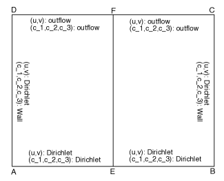
(a) Spatial and temporal convergence test

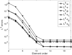
(b) $L^{2}$ errors vs element order

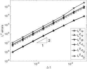
(c) $L^{2}$ errors vs $\Delta t$

Figure 1: Spatial/temporal convergence tests: (a) Problem configuration; (b) $L^{2}$ errors of flow variables versus element order (fixed $\Delta t=0.001$ and $t_{f}=0.1$); (c) $L^{2}$ errors of flow variables versus $\Delta t$ (fixed element order $16$ and $t_{f}=0.1$).

The goal of this subsection is to demonstrate numerically the spatial and temporal convergence rates of the method developed herein using a contrived analytic solution with the proposed N-phase energy-stable open boundary conditions.

Consider the computational domain $\Omega=\overline{ABCD}:=\{(x,y)|0\leq x\leq 2,-1\leq y\leq 1\}$ shown in Fig. 1(a) and a four-fluid (i.e., $N=4$) mixture contained in this domain. We assume the following analytic expressions for the flow variables of this four-phase system,

$$\begin{cases}&u=A_{0}\sin(ax)\cos(\pi y)\sin(\omega_{0}t)\,,\\ &v=-(A_{0}a/\pi)\cos(ax)\sin(\pi y)\sin(\omega_{0}t)\,,\\ &P=A_{0}\sin(ax)\sin(\pi y)\cos(\omega_{0}t)\,,\\ &c_{1}=\cfrac{1}{6}\big{[}1+A_{1}\cos(a_{1}x)\cos(b_{1}y)\sin(\omega_{1}t)\big{]}\,,\\ &c_{2}=\cfrac{1}{6}\big{[}1+A_{2}\cos(a_{2}x)\cos(b_{2}y)\sin(\omega_{2}t)\big{]}\,,\\ &c_{3}=\cfrac{1}{6}\big{[}1+A_{3}\cos(a_{3}x)\cos(b_{3}y)\sin(\omega_{3}t)\big{]}\,,\\ &c_{4}=1-c_{1}-c_{2}-c_{3},\end{cases}$$ (114)

where $(u,v)$ are the two components of the velocity $\bm{u}.$ The above expressions satisfy the system of equations with appropriate choice of the source terms. The source term $\bm{f}$ in (78) is chosen such that the analytic expressions given in (114) satisfy equation (78). We choose $g_{i}\,(i=1,2,3)$ in equations (61) such that (114) satisfies each of the equations (61). The initial conditions (72a)-(72b) are imposed for the velocity and phase field functions, respectively, where $\bm{u}^{\rm in}$ and $c_{i}^{\rm in}\,(i=1,2,3)$ are chosen by letting $t=0$ at the contrived solution (114).

The flow domain $\Omega$ is discretized using two quadrilateral spectral elements of equal size ($\overline{AEFD}$ and $\overline{EBCF}$). On the sides $\overline{AD},\,\overline{AB},\,\overline{BC},$ we impose Dirichlet boundary condition (71) for the velocity field, where the boundary velocity $\bm{w}$ is chosen according to the analytic expressions in (114). For the phase field functions, we impose the wall contact-angle conditions (75) and (76) on $\overline{AD}$ and $\overline{BC},$ and impose the Dirichlet conditions (67) and (74) on $\overline{AB}.$ On the side $\overline{DC}$ we impose the open boundary conditions (79) with $(\theta,\alpha_{1},\alpha_{2})=(1,1,0)$ for the momentum equations, and (75) and (77) for the phase field functions. The source terms $g_{ai},\,g_{bi},\,g_{ci},\,g_{ei},\,c_{bi},\,(i=1,2,3)$ and $\bm{f}_{b}$ therein are chosen such that the contrived solution in (114) satisfies the boundary conditions.

Parameter	Value	Parameter	Value
$a,\,a_{1},\,a_{2},\,a_{3}$	$\pi$	$b_{1},\,b_{2},\,b_{3}$	$\pi$
$A_{0}$	2.0	$A_{1},\,A_{2},\,A_{3}$	1.0
$\omega_{0},\,\omega_{1}$	1.0	$\omega_{2}$	1.2
$\omega_{3}$	0.8	$\eta$, $t_{f}$	0.1
${\tilde{\rho}}_{1}$	1.0	${\tilde{\rho}}_{2}$	3.0
${\tilde{\rho}}_{3}$	2.0	${\tilde{\rho}}_{4}$	4.0
${\tilde{\mu}}_{1}$	0.01	${\tilde{\mu}}_{2}$	0.02
${\tilde{\mu}}_{3}$	0.03	${\tilde{\mu}}_{4}$	0.04
$\sigma_{12}$	$6.236\times 10^{-3}$	$\sigma_{13}$	$7.265\times 10^{-3}$
$\sigma_{14}$	$3.727\times 10^{-3}$	$\sigma_{23}$	$8.165\times 10^{-3}$
$\sigma_{24}$	$5.270\times 10^{-3}$	$\sigma_{34}$	$6.455\times 10^{-3}$
$\alpha_{1},\,\theta$	1.0	$\alpha_{2}$	0
$\delta$	0.05	$d_{0}$	0.2
$m_{0}$	$1.0\times 10^{-5}$	$\mu_{0}$	${\rm max}(\tilde{\mu}_{1},\cdots,\tilde{\mu}_{4})$
$\rho_{0}$	${\rm min}(\tilde{\rho}_{1},\cdots,\tilde{\rho}_{4})$	$\nu_{m}$	$\frac{1}{2}\big{[}{\rm max}\{\frac{\mu_{i}}{\rho_{i}}\}_{i=1}^{4}+{\rm min}\{\frac{\mu_{i}}{\rho_{i}}\}_{i=1}^{4}\big{]}$
$J$ (temporal order)	2	Number of elements	2
$\Delta t$	(varied)	Element order	(varied)

Table 2: Simulation parameter values for the convergence-rate tests.

The numerical algorithm from Section 2.3-2.4 is employed to integrate in time the governing equations for this four-phase system from $t=0$ to $t=t_{f}.$ Then the numerical solution and the exact solution as given by (114) at $t=t_{f}$ are compared, and the errors in the $L^{2}$ norm for various flow variables are computed. All the physical and numerical parameters involved in the simulation of this problem, including the values of constants $A_{i}$ and $\omega_{i}$ ($i=0,\cdots,3$), $a,$ $a_{i}$ and $b_{i}$ ($i=1,2,3$) in the contrived solution (114), are tabulated in Table 2.

Both spatial and temporal convergence tests have been performed to demonstrate the reliability of the proposed algorithm. In the first test, we fix the integration time at $t_{f}=0.1$ and the time step size at $\Delta t=0.001$ ($100$ time steps), and vary the element order systematically between $2$ and $20.$ The same element order has been used for these two spectral elements. Fig. 1(b) plots the numerical errors at $t=t_{f}$ in $L^{2}$ norm for different flow variables as a function of the element order. It is evident that within a specific range of the element order (below around $12$), the errors decrease exponentially when increasing element order, displaying an exponential convergence rate in space. Beyond the element order of about $12,$ the error curves level off as the element order further increases, showing a saturation caused by the temporal truncation error.

In the second test, we fix the integration time at $t_{f}=0.1$ and the element order at a large value $16,$ and vary the time step size systematically between $\Delta t=1.953125\times 10^{-4}$ and $\Delta t=0.025.$ Fig. 1(c) shows the numerical errors at $t=t_{f}$ in $L^{2}$ norm for different variables as a function of $\Delta t$ in logarithmic scales. It can be observed that the numerical errors exhibit a second order convergence rate in time.

The above numerical results indicate that the numerical algorithm developed herein has a spatial exponential convergence rate and a temporal second-order convergence rate for multi-phase problems with energy-stable open boundary conditions.

3.2 A Three-Phase Capillary Wave Problem

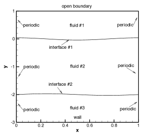
(a) Configuration for three-phase capillary wave problem

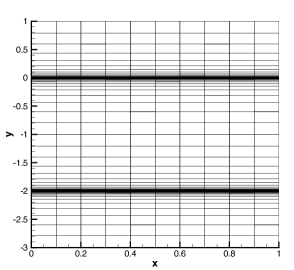
(b) Spectral element mesh

Figure 2: Three-phase capillary wave problem: (a) Computational domain and configuration. (b) Spectral element mesh of $800$ quadrilateral elements.

In this subsection, we use a three-phase capillary wave problem as a benchmark to test the physical accuracy of the current method with energy-stable open boundary conditions.

The problem setting is as follows. We consider three immiscible incompressible fluids contained in an infinite domain (see Fig. 2(a) for an illustration). The upper portion of the domain is occupied by the lightest fluid (fluid $\#1$), and the lower portion of the domain is occupied by the heaviest fluid (fluid $\#3$), and the middle is occupied by fluid $\#2.$ The gravity is assumed to be in the downward direction. The interfaces formed between fluid $\#1$ and fluid $\#2$ (interface $\#1$) and between fluid $\#2$ and fluid $\#3$ (interface $\#2$) are perturbed from their horizontal equilibrium positions by a small amplitude sinusoidal wave form, and start to oscillate at $t=0.$ The objective here is to study the motion of the interfaces over time.

Although this is a three-phase problem, if the two interfaces are far part and the capillary-wave amplitudes are sufficiently small compared with the distance between the interfaces and the dimension of the domain in the vertical direction, the interaction between the interfaces will be weak. The motion of each interface will therefore be essentially the same as that of the interface alone in a two-phase setting, i.e. with the third fluid absent. This allows us to compare qualitatively and quantitatively the numerical results for the three-phase capillary-wave simulations with e.g. Prosperetti’s exact physical solution (see Prosperetti1981 ) for two-phase capillary-wave problems. In Prosperetti1981 an exact time-dependent standing-wave solution to the two-phase capillary-wave problem was derived, given that the two fluids must have matched kinematic viscosities (but their densities and dynamic viscosities can be different).

In what follows, we will simulate the three-phase capillary-wave problem under the following settings: (i) the two interfaces are far apart; (ii) the capillary amplitudes are small compared with both the distance between the interfaces and the vertical dimension of the domain; and (iii) the kinematic viscosity $\nu$ satisfies $\nu=\frac{\tilde{\mu}_{1}}{\tilde{\rho}_{1}}=\frac{\tilde{\mu}_{2}}{\tilde{\rho}_{2}}=\frac{\tilde{\mu}_{3}}{\tilde{\rho}_{3}}$.

Specifically, the simulation setting is illustrated in Fig. 2(a). We consider the computational domain $\Omega=\{(x,y)|0\leq x\leq 1,-3\leq y\leq 1\}.$ The bottom side of the domain is a solid wall of neutral wettability, and the top side is open where the fluid can freely leave (or enter) the domain. On the left and right sides, all the variables are assumed to be periodic at $x=0$ and $x=1.$ The equilibrium positions of the fluid interface $\#1$ and interface $\#2$ are assumed to coincide with $y=0$ and $y=-2$, respectively. The initial perturbed profile of the fluid interface $\#1$ and interface $\#2$ are given by $y=H_{0}\cos(k_{w}x)$ and $y=y_{1}+H_{0}\cos(k_{w}x),$ respectively, where $y_{1}=-2,$ $H_{0}=0.01$ is the initial amplitude, $\lambda_{w}=1$ is the wavelength of the perturbation profiles, and $k_{w}=2\pi/\lambda_{w}$ is the wave number. Note that the initial capillary amplitude $H_{0}$ is small compared with the dimension of the domain in the vertical direction and the distance between the two fluid interfaces. Therefore, the effect of the wall at the domain bottom and the influence of the third fluid on the motion of the fluid interface will be small.

Parameter	Value	Parameter	Value
$H_{0}$	0.01	$k_{w}$ (wave number)	$2\pi$
$\sigma_{ij}\,(1\leq i\neq j\leq 3)$	1.0	$|\bm{g}_{r}|$ (gravity)	1.0
$\tilde{\rho}_{1}$	1.0	$\tilde{\rho}_{2},\,\tilde{\rho}_{3}$	(varied)
$\tilde{\mu}_{1}$	0.01	$\tilde{\mu}_{2}$	$\tilde{\mu}_{1}\frac{\tilde{\rho}_{2}}{\tilde{\rho}_{1}}$
$\tilde{\mu}_{3}$	$\tilde{\mu}_{1}\frac{\tilde{\rho}_{3}}{\tilde{\rho}_{1}}$	$\nu=\frac{\tilde{\mu}_{1}}{\tilde{\rho}_{1}}=\frac{\tilde{\mu}_{2}}{\tilde{\rho}_{2}}=\frac{\tilde{\mu}_{3}}{\tilde{\rho}_{3}}$ (kinematic viscosity)	$0.01$
$\delta$	0.05	$\mu_{0}$	${\rm max}(\tilde{\mu}_{1},\tilde{\mu}_{2},\tilde{\mu}_{3})$
$\theta$	1.0	$\alpha_{1},$ $\alpha_{2}$	$0$
$d_{0}$	0	Element order	8
$\rho_{0}$	${\rm min}(\tilde{\rho}_{1},\cdots,\tilde{\rho}_{3})$	$\nu_{m}$	0.01
$J$ (temporal order)	2	Number of elements	800
$m_{0}$	(varied)	$\eta$	(varied)
$\Delta t$	(varied)

Table 3: Simulation parameter values for the three-phase capillary wave problem.

The computational domain is partitioned with $800$ quadrilateral elements, with $10$ and $80$ elements respectively in $x$ and $y$ directions (Fig. 2(b)). The elements are uniform in the $x$ direction, and are non-uniform and clustered around the regions $-0.012\leq y\leq 0.012$ and $-2.012\leq y\leq-1.988.$ In the simulations, the external body force $\bm{f}$ in equation (78) is set to $\bm{f}=\rho\bm{g}_{r},$ where $\bm{g}_{r}$ is the gravitational acceleration, and the source terms in (61) are set to $g_{i}=0\,(i=1,2).$ On the bottom wall, the boundary condition (71) with $\bm{w}=\bm{0}$ is imposed for the velocity, and the boundary conditions (75) and (76) with $g_{bi}=g_{ci}=0\,(i=1,2)$ are imposed for the phase field functions. On the top domain boundary, the energy-stable open boundary condition (79) with $\bm{f}_{b}=\bm{0}$ and $(\theta,\alpha_{1},\alpha_{2})=(1,0,0)$ is imposed for the momentum equation, and the conditions (75) and (77) with $g_{bi}=g_{ei}=0\,(i=1,2)$ and $d_{0}=0$ are imposed for the phase field functions. The initial velocity is set to zero, and the initial volume fractions are prescribed as follows:

$$\begin{cases}&c_{1}=\cfrac{1}{2}\Big{[}1+\tanh\cfrac{y-H_{0}\cos(k_{w}x)}{\sqrt{2}\eta}\Big{]},\\ &c_{2}=\cfrac{1}{2}\Big{[}\tanh\cfrac{y-y_{1}-H_{0}\cos(k_{w}x)}{\sqrt{2}\eta}-\tanh\cfrac{y-H_{0}\cos(k_{w}x)}{\sqrt{2}\eta}\Big{]},\\ &c_{3}=1-c_{1}-c_{2}.\end{cases}$$ (115)

We list in Table 3 the values for the physical and numerical parameters involved in this problem.

(a) Interface $\#1$ with various element orders

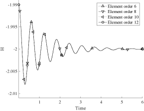
(b) Interface $\#2$ with various element orders

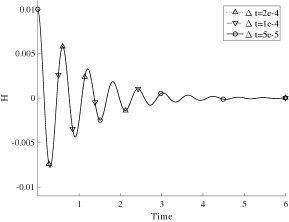
(c) Interface $\#1$ with various $\Delta t$

(d) Interface $\#2$ with various $\Delta t$

Figure 3: Three-phase capillary wave problem (matched density $\tilde{\rho}_{1}=\tilde{\rho}_{2}=\tilde{\rho}_{3}=1$). (a)-(b): Effect of spatial resolution (element order) on the capillary amplitude history. Simulation results are obtained with a fixed time step size $\Delta t=10^{-4},$ interfacial thickness $\eta=0.01,$ mobility $m_{0}=10^{-5}$ and various element orders. (c)-(d): Effect of time step size on the capillary amplitude history. Simulation results are obtained with a fixed element order 8, interfacial thickness $\eta=0.005$, mobility $m_{0}=10^{-5}$ and various time step sizes $\Delta t$.

Let us first focus on a matched density for the three fluids, i.e., $\tilde{\rho}_{1}=\tilde{\rho}_{2}=\tilde{\rho}_{3}=1$, and study the effects of several parameters on the simulation results. We have performed extensive tests to ensure that our simulation results have converged with respect to the spatial and temporal resolutions. Fig. 3(a)-(b) show a spatial resolution test. Here we compare the time histories of the capillary wave amplitudes of the interfaces $\#1$ and $\#2$ obtained with several element orders ranging from 6 to 12 in the simulations. The history curves corresponding to different element orders overlap with one another, suggesting independence of the results with respect to the grid resolution. Fig. 3(c)-(d) show a temporal resolution test. We compare the capillary wave amplitude histories obtained using several time step sizes. The results obviously indicate the convergence with respect to $\Delta t.$

These resolution tests indicate that an element order $8$ and a time step size $\Delta t=10^{-4}$ will be sufficient for the spatial and temporal resolutions with current spectral element mesh. Therefore, the majority of subsequent simulations will be conducted using these parameter values.

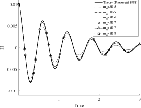
(a) Interface $\#1$ with various $m_{0}$

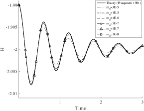
(b) Interface $\#2$ with various $m_{0}$

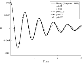
(c) Interface $\#1$ with various $\eta$

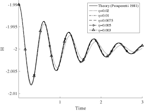
(d) Interface $\#2$ with various $\eta$

Figure 4: Capillary wave problem (matched density $\tilde{\rho}_{1}=\tilde{\rho}_{2}=\tilde{\rho}_{3}=1$). (a)-(b): Comparison of capillary amplitude histories corresponding to different mobility $m_{0}$ values and Prosperetti’s exact solution Prosperetti1981 . Simulation results correspond to a time step size $\Delta t=10^{-4},$ element order $8$, and interfacial thickness $\eta=0.005.$ (c)-(d): Comparison of capillary amplitude histories corresponding to different interfacial thickness $\eta$ values and Prosperetti’s exact solution. Simulation results correspond to a time step size $\Delta t=10^{-4},$ element order $8$, and mobility $m_{0}=5\times 10^{-7}.$

The effect of the mobility coefficient $m_{0}$ on the simulation results is shown by Fig. 4(a)-(b), in which we compare the time histories of the capillary wave amplitudes of the two interfaces obtained with a fixed interfacial thickness scale $\eta=0.005$ and various mobility values ranging between $m_{0}=3\times 10^{-5}$ and $m_{0}=10^{-8}$. The exact physical solution given by Prosperetti1981 for this case is also included in the figure for comparison. It is observed that the computation becomes unstable if $m_{0}$ is too large (larger than around $m_{0}=3\times 10^{-5}$). As $m_{0}$ decreases from $3\times 10^{-5}$ to $10^{-8}$, we initially observe an effect on the amplitude and phase of the history signals obtained from the simulations. But as $m_{0}$ becomes sufficiently small, the difference in the simulated capillary amplitude histories becomes very small, and the history curves converge to the exact solution by Prosperetti1981 . In fact, when $m_{0}$ decreases below $10^{-6}$, the difference between the numerical results and the theoretic solution is negligible.

Fig. 4(c)-(d) show the effect of the interfacial thickness scale $\eta$ on the simulation results. In this figure we compare time histories of the capillary amplitude obtained with the interfacial thickness scale parameter $\eta$ ranging from $0.02$ to $0.003$ with a fixed mobility $m_{0}=5\times 10^{-7}.$ The exact physical solution is also included in the plots. Some influence on the amplitude and the phase of the history curves can be observed as $\eta$ decreases from $0.02$ to $0.01.$ As $\eta$ decreases further to $\eta=0.0075$ and below, on the other hand, the history curves essentially overlap with one another and little difference can be discerned among them, suggesting a convergence of the results with respect to $\eta.$

Figure 5: Three-phase capillary wave (different density ratios): Comparison of time histories of the capillary wave amplitude between simulation and Prosperetti’s exact solution for densities $(\tilde{\rho}_{1},\tilde{\rho}_{2},\tilde{\rho}_{3})=(1,10,10)$ ((a)-(b)), $(1,10,100)$ ((c)-(d)), $(1,100,100)$ ((e)-(f)), $(1,10,1000)$ ((g)-(h)), and $(1,1,1000)$ ((i)-(j)). The simulation results are obtained with a time step size $\Delta t=10^{-4}$ for (a)-(f), $\Delta t=2\times 10^{-5}$ for (g)-(j), an element order 8, interfacial thickness $\eta=0.003$, and mobility $m_{0}=5\times 10^{-7}.$

(a) Interface $\#1$ with $(\tilde{\rho}_{1},\tilde{\rho}_{2},\tilde{\rho}_{3})=(1,10,10)$

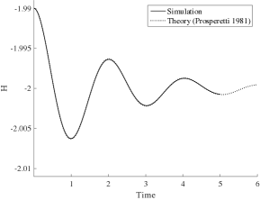
(b) Interface $\#2$ with $(\tilde{\rho}_{1},\tilde{\rho}_{2},\tilde{\rho}_{3})=(1,10,10)$

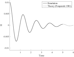
(c) Interface $\#1$ with $(\tilde{\rho}_{1},\tilde{\rho}_{2},\tilde{\rho}_{3})=(1,10,100)$

(d) Interface $\#2$ with $(\tilde{\rho}_{1},\tilde{\rho}_{2},\tilde{\rho}_{3})=(1,10,100)$

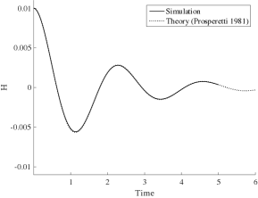
(e) Interface $\#1$ with $(\tilde{\rho}_{1},\tilde{\rho}_{2},\tilde{\rho}_{3})=(1,100,100)$

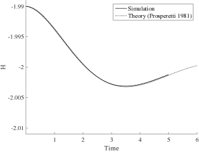
(f) Interface $\#2$ with $(\tilde{\rho}_{1},\tilde{\rho}_{2},\tilde{\rho}_{3})=(1,100,100)$

(g) interface $\#1$ with $(\tilde{\rho}_{1},\tilde{\rho}_{2},\tilde{\rho}_{3})=(1,10,1000)$

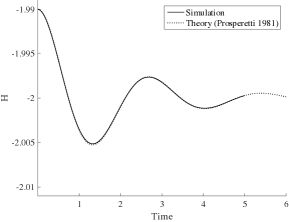
(h) interface $\#2$ with $(\tilde{\rho}_{1},\tilde{\rho}_{2},\tilde{\rho}_{3})=(1,10,1000)$

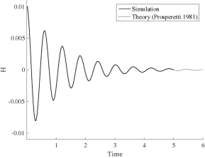
(i) interface $\#1$ with $(\tilde{\rho}_{1},\tilde{\rho}_{2},\tilde{\rho}_{3})=(1,1,1000)$

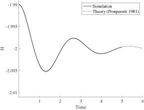
(j) interface $\#2$ with $(\tilde{\rho}_{1},\tilde{\rho}_{2},\tilde{\rho}_{3})=(1,1,1000)$

Let us next investigate the effect of density ratios on the motion of the fluid interfaces. In these tests we vary the densities and dynamic viscosities of the fluid $\#2$ and fluid $\#3$ ($\tilde{\rho}_{2}$, $\tilde{\rho}_{3}$ and $\tilde{\mu}_{2}$, $\tilde{\mu}_{3}$) systematically while the relation $\nu=\frac{\tilde{\mu}_{1}}{\tilde{\rho}_{1}}=\frac{\tilde{\mu}_{2}}{\tilde{\rho}_{2}}=\frac{\tilde{\mu}_{3}}{\tilde{\rho}_{3}}$ is maintained as required by the theoretic solution in Prosperetti1981 . In Fig. 6(f), we show the time histories of the capillary amplitudes corresponding to five density contrasts, $(\tilde{\rho}_{1},\tilde{\rho}_{2},\tilde{\rho}_{3})$ equal (a)-(b): $(1,10,10)$, (c)-(d): $(1,10,100)$, (e)-(f): $(1,100,100)$, (g)-(h): $(1,10,1000)$, and (i)-(j): $(1,1,1000)$, and compare them with the theoretic solutions from Prosperetti1981 . The simulation results are obtained with an element order 8, interfacial thickness $\eta=0.003$, and mobility $m_{0}=5\times 10^{-7}$. The time step size in the simulations is $\Delta t=10^{-4}$ for the plots (a)-(f), and a smaller $\Delta t=2\times 10^{-5}$ for the cases involving $\tilde{\rho}_{3}=1000$ (plots (g)-(j)) in order to ensure the stability of simulations. We observe that the density contrasts have a dramatic effect on the motions of the interfaces, and the dynamics of the two interfaces have become very different. Under the same density ratio, increase in the density values appears to cause the period of oscillation to increase and the attenuation of the oscillation amplitude to be more pronounced; see e.g. Figs. 6(f)(c) and (d). Increase in the density ratio seems to have a similar effect with respect to the oscillation amplitude and period; compare e.g. Figs. 6(f)(a) and (e). It can also be observed that the history curves from the simulations essentially overlap with those of the exact solutions for all the density contrasts and little difference can be perceived, indicating that our method has captured the dynamics of the fluid interfaces correctly.

The three-phase capillary wave problem and in particular the comparisons with Prosperetti’s exact solution for this problem demonstrate that the N-phase formulation with the proposed open boundary conditions and the numerical method developed herein (with $N=3$) have produced physically accurate results for a wide range of density ratios (up to density ratio $1000$ tested here).

3.3 Interaction of Two Liquid Jets in Ambient Water

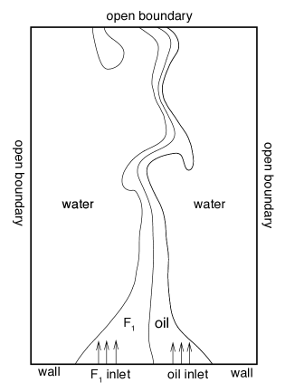
Figure 6: Configuration of the interaction of $F_{1}$-oil jets in water.

In this subsection, we test the proposed open boundary conditions and the numerical method by considering the interactions of two fluid jets in an infinite expanse of ambient water. The two jets consists of two different liquids. One of the jets is oil, and the other is a liquid referred to as “F₁”. The F₁ liquid is assumed to be lighter than water and immiscible with both oil and water. This test problem involves multiphase inflow/outflow boundaries. How to deal with such boundaries is critical to the successful simulation of this problem.

Specifically, we consider a rectangular flow domain $\Omega=\{(x,y)|-0.5L\leq x\leq 0.5L,0\leq y\leq 1.5L\}$ where $L=6cm$, as shown in Fig. 6. The bottom side of the domain ($y=0$) is a solid wall of neutral wettability. The other three sides of the domain are all open where the fluids can enter or leave the domain freely. The domain initially contains water inside. The bottom wall has two orifices, each having a diameter $0.2L$. The centers of two orifices are located at $(x_{1},y_{1})=(-0.2L,0)$ and $(x_{2},y_{2})=(0.2L,0)$, respectively. A jet of a certain fluid labeled by F₁ enters the domain through the left orifice, and a jet of oil is introduced into the domain through the right orifice. The gravity $\bm{g}_{r}$ is assumed to point downward ($-y$ direction). The configuration of this problem models the motion of the $F_{1}$ jet and the oil jet in an infinite expanse of water. The two jets rise through the water due to buoyancy, interact with each other, and move out of the domain through the open boundaries. The goal here is to investigate the long-time behavior of this three-phase system.

Density [$kg/m^{3}$]:	$F_{1}$ - 600	water - 998.2071	oil - 400 or 100
Dynamic viscosity [$kg/(m\cdot s)$]:	$F_{1}$ - $2\times 10^{-2}$	water - $1.002\times 10^{-3}$	oil - $9.15\times 10^{-2}$
Surface tension [$kg/s^{2}$]:	$F_{1}/$water - $4.5\times 10^{-2}$	$F_{1}/$oil - $4.8\times 10^{-2}$	oil/water - $4.4\times 10^{-2}$
Gravity [$m/s^{2}$]:	9.8

Table 4: Physical property values of fluids $F_{1}$, water and oil.

The physical properties (including the densities, viscosities, pair-wise surface tensions) of F₁, water, and oil employed in this problem, as well as the gravitational acceleration, are listed in Table 4. We choose $L=6cm$ as the length scale, the density of F₁ as the density scale $\varrho_{d},$ and the centerline velocity at the orifices as the velocity scale $U_{0}$. Then the problem is non-dimensionalized based on Table 1. In what follows, all physical and numerical parameters have been properly normalized.

Parameter	Value	Parameter	Value
$x_{1}$	-0.2	$x_{2}$	0.2
$R$	0.1	$d_{0}$	0.5
$\alpha_{1},$ $\theta$	1	$\alpha_{2}$	0
$\delta$	0.01	$\mu_{0}$	${\rm max}(\tilde{\mu}_{1},\tilde{\mu}_{2},\tilde{\mu}_{3})$
$\rho_{0}$	${\rm min}(\tilde{\rho}_{1},\cdots,\tilde{\rho}_{3})$	$\nu_{m}$	$1.56\times 10^{-2}$
$m_{0}$	$1\times 10^{-8}$	$\eta$	0.01
$J$ (temporal order)	2	Number of elements	600
$\Delta t$	$2\times 10^{-5}$	Element order	6

Table 5: Simulation parameter values for the interaction of two liquid jets in ambient water.

In the numerical experiments, we specify $F_{1}$, water and oil as the first, second, and the third fluids, with the normalized densities $\tilde{\rho}_{1}$, $\tilde{\rho}_{2}$, and $\tilde{\rho}_{3},$ respectively. We discretize the computational domain with a mesh of $600$ quadrilateral elements of uniform size, with $20$ elements in the $x$ direction and $30$ elements in the $y$ direction. The element order is $6$ for all the elements. The time step size is chosen as $\Delta t=2\times 10^{-5}$ and all the simulation results afterwards are obtained with interfacial thickness $\eta=0.01$, and mobility $m_{0}=10^{-8}.$ To balance the gravity of the water, in the simulations we also apply an external pressure gradient pointing upward ($y$ direction) in the whole domain with a magnitude $\rho_{w}|\bm{g}_{r}|,$ where $\rho_{w}$ is the density of water. As a result, the region occupied by water has no net external body force exerted on it. The external body force $\bm{f}$ in equation (78) is set to $\bm{f}=\rho\bm{g}_{r}-\tilde{\rho}_{2}\bm{g}_{r},$ where $\tilde{\rho}_{2}$ and $\bm{g}_{r}$ are the normalized density of water and gravitational acceleration, respectively. The source term in (61) are set to $g_{i}=0\,(i=1,2).$ On the bottom wall (excluding the fluid inlets), we impose the Dirichlet boundary condition (71) for the velocity with $\bm{w}=\bm{0}$ and the boundary conditions (75) and (76) with $g_{bi}=g_{ci}=0\,(i=1,2)$ for the phase field variables. At the F₁ and oil inlets, we assume a parabolic profile for the velocity, i.e. $\bm{w}=(0,w_{y})$ in (71) with

$$w_{y}=U_{0}\left[1-\Big{(}\frac{x-x_{1}}{R}\Big{)}^{2}\right],\;\;x\in(x_{1}-R,x_{1}+R);\;\;\;w_{y}=U_{0}\left[1-\Big{(}\frac{x-x_{2}}{R}\Big{)}^{2}\right],\;\;x\in(x_{2}-R,x_{2}+R),\quad$$ (116)

where $R=0.1L$ is the radius of the orifice and $U_{0}=24.49cm/s$ is the centerline velocity at the orifices. For the phase field functions we impose the following distributions at the two fluid inlets,

$$c_{1}=1,\;\;c_{2}=0,\ x\in(x_{1}-R,x_{1}+R);\;\;\;c_{1}=0,\;\;c_{2}=0,\;\;x\in(x_{2}-R,x_{2}+R).$$ (117)

This distribution means that only the F₁ fluid is present at the left inlet, and only the oil is present at the right inlet. On the other three sides, we impose the open boundary conditions (79), (75) and (77), respectively for the velocity and the phase field functions, where $\bm{f}_{b}=\bm{0}$, $g_{bi}=g_{ei}=0,\ (i=1,2)$, and $(\theta,\alpha_{1},\alpha_{2})=(1,1,0)$. In (79), the $d_{0}$ value is determined by the following procedure. We first perform a preliminary simulation using $d_{0}=0$, and then estimate a convection velocity scale at the outlet boundary. The $d_{0}$ is then set as the inverse of this convection velocity scale. For the current problem, $d_{0}$ is set to $0.5$ based on this procedure.

The initial velocity is set to zero, and the initial volume fractions are set as follows:

$$\begin{cases}&c_{1}=\big{[}H(x-x_{1}+R)-H(x-x_{1}-R)\big{]}\big{[}H(y)-H(y-2R)\big{]},\\ &c_{2}=1-c_{1}-c_{3},\\ &c_{3}=\big{[}H(x-x_{2}+R)-H(x-x_{2}-R)\big{]}\big{[}H(y)-H(y-2R)\big{]},\end{cases}$$ (118)

where $H(x)$ is the Heaviside step function, taking the unit value if $x\geqslant 0$ and vanishing otherwise. It should be noted that these initial distributions for the phase field functions and the velocity have no effect on the long-term behavior of the system. Any transient influence will be convected out of the domain eventually. The values for the simulation parameters in this problem are collected in Table 5.

We have considered two cases, corresponding to two different density values for the oil: $400kg/m^{3}$ in the first case, and $100kg/m^{3}$ in the second case.

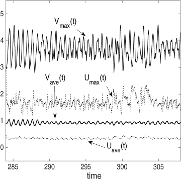
Figure 7: Time histories of the maximum and average velocity magnitudes for the case $(\tilde{\rho}_{1},\tilde{\rho}_{2},\tilde{\rho}_{3})=(1,1.664,0.667)$, showing that the flow has reached a statistically stationary state.

Let us first consider the case with an oil density $400kg/m^{3}$. The normalized densities for $F_{1},$ water and oil are $(\tilde{\rho}_{1},\tilde{\rho}_{2},\tilde{\rho}_{3})=(1,1.664,0.667)$ for this case. We have performed a long-time simulation of the problem so that the flow has reached a statistically stationary state. We have monitored the following maximum magnitudes $U_{\rm max},V_{\rm max}$ and average magnitudes $(U_{\rm ave},V_{\rm ave})$ of the $x$ and $y$ components of velocity at each time step:

$$U_{\rm max}(t)={\rm max}_{\bm{x}\in\Omega}|u(\bm{x},t)|,\quad V_{\rm max}(t)={\rm max}_{\bm{x}\in\Omega}|v(\bm{x},t)|;$$ (119)

$$U_{\rm ave}(t)=\Big{(}\frac{1}{V_{\Omega}}\int_{\Omega}|u|^{2}d{\Omega}\Big{)}^{\frac{1}{2}},\quad V_{\rm ave}(t)=\Big{(}\frac{1}{V_{\Omega}}\int_{\Omega}|v|^{2}d{\Omega}\Big{)}^{\frac{1}{2}},$$

where $V_{\Omega}=\int_{\Omega}d\Omega$ is the volume of the domain. Fig. 7 shows a temporal window of the time histories of these velocity magnitudes. It can be observed that while these physical quantities fluctuate over time, their fluctuations are all around some constant mean values, indicating that the flow has reached a statistically stationary state.

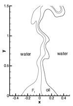
(a) $t=303.62$

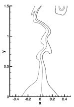
(b) $t=303.72$

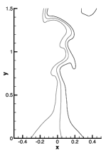
(c) $t=303.82$

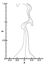
(d) $t=303.92$

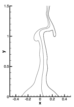
(e) $t=304.02$

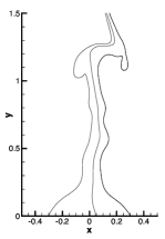
(f) $t=304.12$

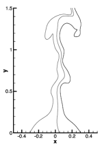
(g) $t=304.22$

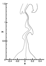
(h) $t=304.32$

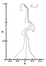
(i) $t=304.42$

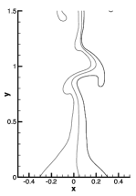
(j) $t=304.52$

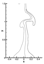
(k) $t=304.62$

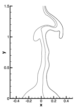
(l) $t=304.72$

Figure 8: Temporal sequence of snapshots of fluid interfaces, visualized by the volume-fraction contours $c_{i}=1/2\,(i=1,2,3),$ showing the interaction of two liquid jets of $F_{1}$ and oil in water, with the normalized densities $(\tilde{\rho}_{1},\tilde{\rho}_{2},\tilde{\rho}_{3})=(1,1.664,0.667)$. The jet inlets are centered at $x=-0.2,\,0.2,$ respectively with radius $0.1$.

We look into the dynamical characteristics of the fluid $F_{1}$ and oil jets in water. Fig. 8 shows a temporal sequence of snapshots of the fluid interfaces, visualized by contours of the volume fractions $c_{i}=1/2\,(i=1,2,3)$ for the three fluids. First we observe that at the bottom wall the F₁ fluid and the oil coming out of the orifices spread on the wall and fill up the space in between. As a result, the two fluids touch each other on the bottom wall and form a compound oil-$F_{1}$ jet. Note that the base of the compound oil-F₁ jet is broader than the combined size of the two orifices. The compound jet exhibits distinct characteristics in different regions. In the region near the orifices ($y/L\lesssim 0.5$ in this case), the compound jet maintains a relatively stable configuration. The jet tapers off along the vertical direction in this region, due to the velocity increase caused by the buoyancy. This is reminiscent of the behavior of a single oil jet in ambient water studied in Dong2014obc . Beyond this stable region, the compound jet exhibits a wavy pattern in its profile. The jet diameter modulates along the vertical direction, and bulges form around the jet continually and periodically (Figs. 8(a)-(b), (f)-(h)) due to a Plateau-Rayleigh instability Plateau1873 ; Rayleigh1892 . Further downsteam, the dynamics of the jet becomes very complicated. The compound jet and the bulges along its profile appear to fold back in certain regions at times, causing very large deformations of the jet; see e.g. Figs. 8(e)-(g) and (j)-(l). We observe that the regions occupied by the F₁ fluid and by the oil in the compound jet are not symmetric. It can also be observed that our method allows the compound oil-F₁ jet and the fluid interfaces to exit the domain through the open boundary in a fairly natural fashion; see e.g. Figs. 8(a)-(d) and (h)-(k).

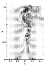
(a) $t=303.62$

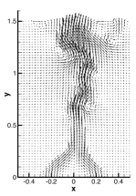
(b) $t=303.72$

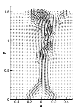
(c) $t=303.82$

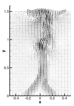
(d) $t=303.92$

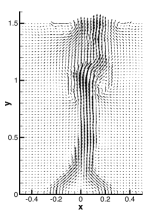
(e) $t=304.02$

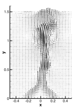
(f) $t=304.12$

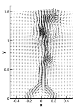
(g) $t=304.22$

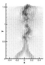
(h) $t=304.32$

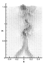
(i) $t=304.42$

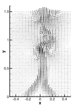
(j) $t=304.52$

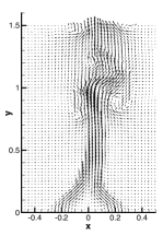
(k) $t=304.62$

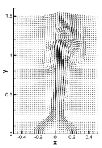
(l) $t=304.72$

Figure 9: Temporal sequence of snapshots of velocity distributions of two liquid jets in water with normalized densities $(\tilde{\rho}_{1},\tilde{\rho}_{2},\tilde{\rho}_{3})=(1,1.664,0.667)$. Velocity vectors are plotted on every eighth quadrature points in each direction within each element.

Fig. 9 shows a temporal sequence of snapshots of the velocity fields of this flow, taken at identical time instants as those of the volume-fraction plots of Fig. 8. Several characteristics are evident from these plots. First, the velocity patterns clearly indicate that the streams of the F₁ fluid and the oil bend toward each other after exiting the orifices, and merge to form a flow stream of the compound jet. The velocity in the region between the two orifices near the wall is very weak. Note that this region is occupied by the F₁ and the oil. Second, the region occupied by the compound jet stream, as shown by the velocity patterns, is wider than the actual region the material oil/F₁ occupy (see Fig. 8), especially in the regions more downstream and near the upper open boundary. This suggests that the water in the vicinity of compound $F_{1}$-oil jet has been accelerated to form a wider high-speed region. Third, the jet stream exhibits a lateral spread along the streamwise direction, as can be observed from the velocity patterns, and pairs of vortices can be observed to form along the jet profile. These vortices reside behind the $F_{1}$-oil bulges, form periodically as new bulges emerge, and travel downstream along with the bulges. Finally, we note that on the side boundaries the velocity generally points into the domain, indicating that the water has in general been sucked into the domain from both sides. The velocity patterns of Fig. 9 indicate that the method developed herein allows the flow to pass through the open/outflow boundaries in a smooth and natural way.

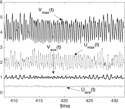
Figure 10: Two liquid jets in water: time histories of the maximum and average velocity magnitudes with normalized densities $(\tilde{\rho}_{1},\tilde{\rho}_{2},\tilde{\rho}_{3})=(1,1.664,0.1664)$, showing that the flow has reached a statistically stationary state.

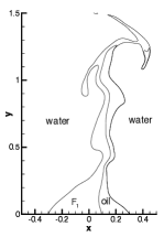
(a) $t=426.92$

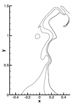
(b) $t=427.02$

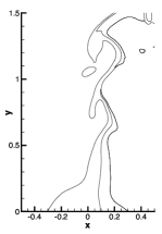
(c) $t=427.12$

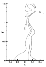
(d) $t=427.22$

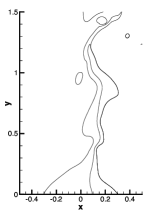
(e) $t=427.32$

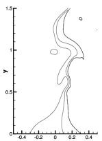
(f) $t=427.42$

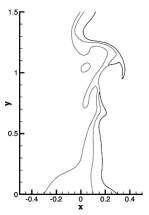
(g) $t=427.52$

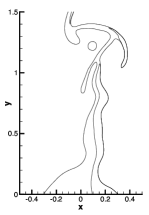
(h) $t=427.62$

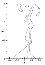
(i) $t=427.72$

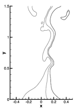
(j) $t=427.82$

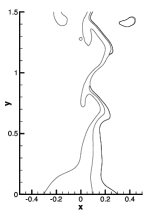
(k) $t=427.92$

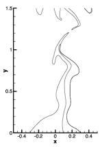
(l) $t=428.02$

Figure 11: Temporal sequence of snapshots of fluid interfaces, visualized by the volume-fraction contours $c_{i}=1/2\,(i=1,2,3)$, showing the interaction of two liquid jets in water, with the normalized densities $(\tilde{\rho}_{1},\tilde{\rho}_{2},\tilde{\rho}_{3})=(1,1.664,0.167)$.

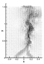
(a) $t=426.92$

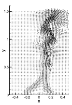
(b) $t=427.02$

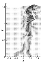
(c) $t=427.12$

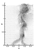
(d) $t=427.22$

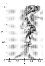
(e) $t=427.32$

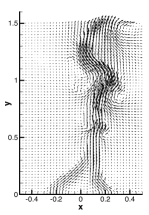
(f) $t=427.42$

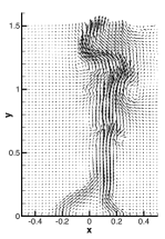
(g) $t=427.52$

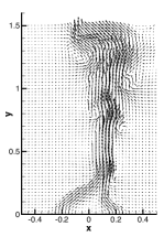
(h) $t=427.62$

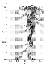
(i) $t=427.72$

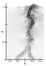
(j) $t=427.82$

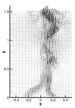
(k) $t=427.92$

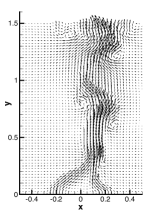
(l) $t=428.02$

Figure 12: Temporal sequence of snapshots of velocity distributions of two liquid jets in water problem, with normalized densities $(\tilde{\rho}_{1},\tilde{\rho}_{2},\tilde{\rho}_{3})=(1,1.664,0.167).$ Velocity vectors are plotted on every eighth quadrature points in each direction within each element.

Let us next consider the second case, with an oil density $100kg/m^{3}$. The normalized densities for $F_{1}$, water and oil are $(\tilde{\rho}_{1},\tilde{\rho}_{2},\tilde{\rho}_{3})=(1,1.664,0.1664)$. All the other physical parameters are the same as in the first case. Long-time simulations have been performed for this case, and Fig. 10 shows time histories of the maximum and average velocity magnitudes defined in (119), indicating that the flow has reached a statistically stationary state. Figs. 11 and 12 are the temporal sequence of snapshots of the fluid interfaces and the velocity fields corresponding to this case. The general characteristics of the dynamics of jets and the velocity distributions are similar to those of the first case. But some marked differences can be noticed. The compound oil-F₁ jet becomes notably more unstable because of the stronger buoyancy force in the oil region. We observe a smaller region ($y/L\gtrsim 0.3$) with a relatively stable jet profile near the base of the jet. Downstream of this region, the deformation of the jet profiles is much more pronounced than in the first case, and droplets of the oil and F₁ fluid are observed to break off from the compound jet. The velocity field in the region occupied by the compound oil-F₁ jet appear stronger and more violent compared with that of the first case. Vortices and backflows can also be observed at the upper or side boundaries at times; see Fig. 12(a)-(d). The results indicate that with the proposed method the fluid interfaces and the flow structures appear to be able to pass through the open/outflow boundaries smoothly and seamlessly.

4 Concluding Remarks

We have developed a set of effective outflow/open boundary conditions (and also inflow boundary conditions) for simulating multiphase flows consisting of $N$ ($N\geqslant 2$) immiscible incompressible fluids in domains involving outflow and inflow boundaries. These boundary conditions are designed to satisfy two properties: energy stability and reduction consistency. The proposed boundary conditions ensure that, at the continuum level, their contributions to the N-phase energy balance will not cause the total system energy to increase over time, regardless of the flow state at the outflow/open boundary. In other words, this property holds even in situations where strong vortices or backflows occur at the outflow/open boundary. This is the reason why the proposed boundary conditions are effective in overcoming the backflow instability in N-phase flow problems. The reduction consistency of the boundary conditions is a physical consistency requirement for N-phase formulations Dong2017 . This property means that the boundary conditions honor the inherent equivalence relations between N-phase systems and the resultant smaller multiphase systems when some fluid components were absent from the N-phase system.

We have also presented an efficient numerical algorithm for the proposed outflow/inflow boundary conditions together with the N-phase governing equations. The main issue lies in the numerical treatments of the inertia term in the open boundary conditions for the phase field equations and the variable viscosity in the open boundary condition for the momentum equation. With appropriate reformulations and treatments of such terms in our algorithm, the computations for different flow variables and the computations for different phase field variables have been completely de-coupled. The proposed algorithm involves only the solution of a number of Helmholtz-type equations within each time step. The linear algebraic systems resulting from discretizations involve only constant and time-independent coefficient matrices, which can be pre-computed, even though large density contrasts and large viscosity contrasts may be present in the N-phase system. These characteristics make the algorithm computationally very efficient and attractive.

We have tested the proposed method with extensive numerical experiments for several problems involving multiple fluid components and in domains with outflow and inflow boundaries. In particular, we have compared in detail our simulation results for the three-phase capillary wave problem with Prosperetti’s exact physical solution Prosperetti1981 under various physical and simulation parameters. These comparisons demonstrate that the proposed method produces physically accurate results.

Multiphase flows involving inflow/outflow boundaries are an important class of problems, which have widespread applications in oil/gas industries, carbon sequestration, microfluidics and optofluidics HuppertN2014 ; PsaltisQY2006 ; RodriguezSMG2015 . These problems are also critical to the study of long-time behaviors and statistical features of multiphase flows. The key technique for simulating multiphase inflow/outflow problems lies in how to deal with the multiphase outflow/open boundaries. The method developed in the current work provides an effective and powerful tool for simulating this class of problems. We anticipate that it will be useful and instrumental in the investigation of long-time statistics of multiphase problems and in the development a number of related areas.

While the outflow/open boundary conditions proposed here ensure the energy stability of the N-phase system at the continuum level, this property is not guaranteed by the numerical algorithm presented here at the discrete level. The current algorithm is only conditionally stable, and requires sufficient spatial resolution and small enough time step size to achieve stable and accurate simulations. An interesting question is how to devise an algorithm for these outflow/open boundary conditions together with the N-phase governing equations to guarantee the energy stability at the discrete level. This problem seems to be highly non-trivial. It would be an interesting problem to contemplate for future research.

References

• [1] H. Abels, H. Garcke, and G. Grün. Thermodynamically consistent, frame indifferent diffuse interface models for incompressible two-phase flows with different densities. Mathematical Models and Methods in Applied Sciences, 22:1150013, 2012.
• [2] A. Albadawi, D.B. Donoghue, A.J. Robinson, D.B. Murray, and Y.M.C. Delaure. Influence of surface tension implementation in volume of fluid and coupled volume of fluid with level set methods for bubble growth and detachment. International Journal of Multiphase Flow, 53:11–28, 2013.
• [3] J. Rodriguez-Rodriguez amd A. Sevilla, C. Martinez-Bazan, and J.M. Gordillo. Generation of microbubbles with applications to industry and medicine. Annual Review of Fluid Mechanics, 47:405–429, 2015.
• [4] D.M. Anderson, G.B. McFadden, and A.A. Wheeler. Diffuse-interface methods in fluid mechanics. Annual Review of Fluid Mechanics, 30:139–165, 1998.
• [5] L. Banas and R. Nurnberg. Numerical approximation of a non-smooth phase-field model for multicomponent incompressible flow. ESAIM: Mathematical Modeling and Numerical Analysis, 51:1089–1117, 2017.
• [6] F. Boyer and C. Lapuerta. Study of a three component Cahn-Hilliard flow model. ESAIM: Mathematical Modeling and Numerical Analysis, 40:653–687, 2006.
• [7] F. Boyer, C. Lapuerta, S. Minjeaud, B. Piar, and M. Quintard. Cahn-Hilliard/Navier-Stokes model for the simulation of three-phase flows. Transport in Porous Media, 82:463–483, 2010.
• [8] F. Boyer and S. Minjeaud. Hierarchy of consistent n-component Cahn-Hilliard systems. Mathematical Models and Methods in Applied Sciences, 24:2885–2928, 2014.
• [9] J.L. Desmarais and J.G.M. Kuerten. Open boundary conditions for the diffuse interface model in 1-D. Journal of Computational Physics, 263:393–418, 2014.
• [10] S. Dong. On imposing dynamic contact-angle boundary conditions for wall-bounded liquid-gas flows. Computer Methods in Applied Mechanics and Engineering, 247–248:179–200, 2012.
• [11] S. Dong. An efficient algorithm for incompressible N-phase flows. Journal of Computational Physics, 276:691–728, 2014.
• [12] S. Dong. An outflow boundary condition and algorithm for incompressible two-phase flows with phase field approach. Journal of Computational Physics, 266:47–73, 2014.
• [13] S. Dong. A convective-like energy-stable open boundary condition for simulations of incompressible flows. Journal of Computational Physics, 302:300–328, 2015.
• [14] S. Dong. Physical formulation and numerical algorithm for simulating N immiscible incompressible fluids involving general order parameters. Journal of Computational Physics, 283:98–128, 2015.
• [15] S. Dong. Wall-bounded multiphase flows of $N$ immiscible incompressible fluids: consistency and contact-angle boundary condition. Journal of Computational Physics, 338:21–67, 2017.
• [16] S. Dong, G.E. Karniadakis, and C. Chryssostomidis. A robust and accurate outflow boundary condition for incompressible flow simulations on severely-truncated unbounded domains. Journal of Computational Physics, 261:83–105, 2014.
• [17] S. Dong and J. Shen. A time-stepping scheme involving constant coefficient matrices for phase field simulations of two-phase incompressible flows with large density ratios. Journal of Computational Physics, 231:5788–5804, 2012.
• [18] S. Dong and J. Shen. A pressure correction scheme for generalized form of energy-stable open boundary conditions for incompressible flows. Journal of Computational Physics, 291:254–278, 2015.
• [19] S. Dong and X. Wang. A rotational pressure correction scheme for incompressible two-phase flows with open boundary conditions. PLoS One, 11(5):e0154565, 2016.
• [20] P.M. Gresho. Incompressible fluid dynamics: some fundamental formulation issues. Annual Review of Fluid Mechanics, 23:413–453, 1991.
• [21] M. Heida, J. Malek, and K.R. Rajagopal. On the development and generalization of Cahn-Hilliard equations within a thermodynamic framework. Zeitschrift für angewandte Mathematik und Physik, 63:145–169, 2012.
• [22] H.E. Huppert and J.A. Neufeld. The fluid mechanics of carbon dioxide sequestration. Annual Review of Fluid Mechanics, 46:255–272.
• [23] G.E. Karniadakis and S.J. Sherwin. Spectral/hp element methods for computational fluid dynamics, 2nd edition. Oxford University Press, 2005.
• [24] J. Kim. Phase-field models for multi-component fluid flows. Communications in Computational Physics, 12:613–661, 2012.
• [25] J. Kim and J. Lowengrub. Phase field modeling and simulation of three-phase flows. Interfaces and Free Boundaries, 7:435–466, 2005.
• [26] M. Lenzinger and B. Schweizer. Two-phase flow equations with outflow boundary conditions in the hydrophobic-hydrophilic case. Nonlinear Analysis, 73:840–853, 2010.
• [27] J. Li and Q. Wang. A class of conservative phase field models for multiphase fluid flows. Journal of Applied Mechanics, 81:021004, 2014.
• [28] C. Liu and J. Shen. A phase field model for the mixture of two incompressible fluids and its approximation by a fourier-spectral method. Physica D, 179:211–228, 2003.
• [29] Q. Lou, Z. Guo, and B. Shi. Evaluation of outflow boundary conditions for two-phase lattice Boltzmann equation. Physical Review E, 87:063301, 2013.
• [30] J. Lowengrub and L. Truskinovsky. Quasi-incompressible Cahn-Hilliard fluids and topological transitions. Proceedings of the Royal Society A, 454:2617–2654, 1998.
• [31] S.T. Munkejord. Partially-reflecting boundary conditions for transient two-phase flow. Communications in Numerical Methods in Engineering, 22:781–795, 2006.
• [32] J. Plateau. Experimental and Theoretical Steady State of Liquids Subjectted to Nothing but Molecular Forces. Paris: Gauthiers-Villars, 1873.
• [33] A. Prosperetti. Motion of two superposed viscous fluids. Physics of Fluids, 24:1217–1223, 1981.
• [34] D. Psaltis, S.R. Quake, and C. Yang. Developing optofluidic technology through the fusion of microfluidics and optics. Nature, 442:381–386, 2006.
• [35] L. Rayleigh. On the theory of surface forces II. Philosophical Magazine, 33:209, 1892.
• [36] R.L. Sani and P.M. Gresho. Resume and remarks on the open boundary condition minisymposium. International Journal for Numerical Methods in Fluids, 18:983–1008, 1994.
• [37] S.J. Sherwin and G.E. Karniadakis. A triangular spectral element method: applications to the incompressible Navier-Stokes equations. Computer Methods in Applied Mechanics and Engineering, 123:189–229, 1995.
• [38] G. Son. A numerical method for incompressible two-phase flows with open or periodic boundaries. Numerical Heat Transfer B, 39:45–60, 2001.
• [39] S. Wu and J Xu. Multiphase allen-cahn and cahn-hilliard models and their discretizations with the effect of surface tensions. Journal of Computational Physics, 343:10–32, 2017.
• [40] X. Yang, J. Zhao, Q. Wang, and J. Shen. Numerical approimations for a three-component cahn-hilliard phase-field model based on the invariant energy quadratization method. Mathematical Models and Methods in Applied Sciences, 27:1993–2030, 2017.
• [41] P. Yue, J.J. Feng, C. Liu, and J. Shen. A diffuse-interface method for simulating two-phase flows of complex fluids. Journal of Fluid Mechanics, 515:293–317, 2004.
• [42] Q. Zhang and X.P. Wang. Phase field modeling and simulation of three-phase flow on solid surfaces. Journal of Computational Physics, 319:79–107, 2016.
• [43] J. Zhao, H. Li, Q. Wang, and X. Yang. Decoupled energy stable schemes for a phase field model of a three-phase incompressible viscous fluid flow. Journal of Scientific Computing, 70:1367–1389, 2017.
• [44] X. Zheng and S. Dong. An eigen-based high-order expansion basis for structured spectral elements. Journal of Computational Physics, 230:8573–8602, 2011.