Linear Response for dynamical systems with additive noise

Abstract.

We show a linear response statement for fixed points of a family of Markov operators which are perturbations of mixing and regularizing operators. We apply the statement to random dynamical systems on the interval given by a deterministic map $T$ with additive noise (distributed according to a bounded variation kernel). We prove linear response for these systems, also providing explicit formulas both for deterministic perturbations of the map $T$ and for changes in the noise kernel. The response holds with mild assumptions on the system, allowing the map $T$ to have critical points, contracting and expanding regions. We apply our theory to topological mixing maps with additive noise, to a model of the Belozuv-Zhabotinsky chemical reaction and to random rotations. In the final part of the paper we discuss the linear request problem for these kind of systems, determining which perturbations of $T$ produce a prescribed response.

1. Introduction

It is of major interest, both in pure mathematics and in applications, to understand how the statistical properties of a physical system change when it suffers from perturbations.

Sometimes small changes in the system produce small changes in its statistical behavior, and the system is said to be statistically stable, sometimes small changes lead to catastrophic events. Beyond the qualitative statistical stability, sometimes it is possible to get a quantitative understanding of the response of the system to small perturbations, both in magnitude and direction. This understanding can be achieved in many cases of systems having linear response to perturbations. As a matter of fact, the linear response of the system with respect to a perturbation can be described by a suitable derivative, representing the rate of change of the relevant (physical, stationary) invariant measure of the system with respect to the perturbation. Hence, the response describes the first order change of the equilibrium state allowing us to get information about its robustness or sensitivity to change in its parameters.

A concrete application of the above ideas can be found in modern geophysics: if a climate model relies on a parameter which corresponds to external forcing, it is relevant to study the stability of equilibrium states and their evolution, informally “the directions of change” with respect to such forcing. This includes information on the behavior of macroscopic objects such as persistent atmospheric or oceanic currents, large vortices, gyre and streams (see [43, 48] for more details or [27] for an inspirational review and further references). Furthermore, when considering the management of a chaotic or complex system one is led to consider an inverse problem related to the linear response: is it possible to realize a specific change of the equilibrium state by controlling the perturbation? Is there an “optimal” way of doing so? (See [23, 34, 6, 41] and Section 6 for a more detailed introduction to this control problem). We will investigate this family of questions specifically in the case of a random dynamical system given by a deterministic map with additive noise.

While the analysis of the linear response of a system may provide a lot of information, it is a fact that not all systems are well behaved with respect to perturbations. In particular not all dynamical systems are even “statistically stable” . The identity map is an example of a system which is not stable under any reasonable formal definition of statistical stability. On the other hand, many systems of applied and theoretical interest are stable. The literature about qualitative statistical stability in dynamical systems is vast, see the introduction of [4] for an historical account on the notion of statistical stability, see [2, 3] and references therein for more recent results. Quantitative estimates show the existence of systems which are statistically stable but have a response to perturbation of orders of magnitude larger than the perturbation itself. The stationary measure may vary just with Hölder modulus of continuity, or even worse, see e.g. [14, 19, 21, 22, 55, 25, 35].

It is worth to remark that a general relation holds, between this modulus of continuity and the speed of convergence to equilibrium of the system (see [22, 21] see also [45] for earlier results limited to Markov chains).

The results discussed so far mostly regard the stability of deterministic systems under deterministic perturbation. In fact, the statistical stability of deterministic systems under small random perturbations is called stochastic stability and it has been studied quite extensively. Early results on piecewise monotonic transformation with some regularity assumption on both the transformation and the invariant measures were already obtained by Keller [31]. The book [33] provides an excellent starting point for the study of the subject.

Concerning systems having Linear Response, several results have been proved for deterministic perturbations of deterministic dynamical systems. Starting with Ruelle, it is known that in smooth, uniformly hyperbolic systems the physical invariant measure changes smoothly and a formula for such differentiation can be obtained (see [51]). Similar results can be proved in some non uniformly expanding or hyperbolic cases (see e.g. [10, 11, 15, 18, 9, 12, 37, 55]). On the other hand, it is known that the linear response does not always hold, due to the lack of regularity of the system, of the perturbation or the lack of sufficient hyperbolicity (see [10, 14, 55, 22]). An example of linear response for small random perturbations of deterministic systems (which uses ideas similar to what we will implement here) is produced in [46]. The survey [13] has exhaustive list of classical references on the subject at hand. The reader interested in seeing linear response from a point of view closer to physics can consult [47, 1]. Rigorous numerical approaches for the computation of the linear response are available, to some extent, both for deterministic and random systems (see [7, 49]).

About linear response of random dynamical systems in general, less is known. As it is common in literature, by random system we mean a system defined by a random dynamics which might, or might not, involve a deterministic part e.g. a dynamics defined only by a transition operator acting on probability distributions versus a random choice between deterministic maps. To study the response of such systems we may perturb any of its defining components and look at the change in the resulting statistical properties. Results for this kind of systems were proved in [30], where the technical framework was adapted to stochastic differential equations. Moreover, there is a recent work [8] proving linear response for a class of random uniformly and non uniformly expanding systems. See Remark 16 for a detailed comparison between the present work, and these two closely related results.

In the random case, like in the deterministic case, a fruitful strategy to study the stability of a system, relies on noticing that the stationary measures of interest are fixed points of the transfer operators associated to the system we consider; thus, linear response statements or quantitative stability results can be proved by first proving perturbation theorems for suitable operators as done in [30, 20, 52, 22, 32, 46].

In this paper we apply this general strategy to an important class of random dynamical systems. We prove a general fixed point stability result and linear response for a class of Markov operators satisfying mild assumptions adapted to random dynamical systems where the unperturbed operators have both mixing and regularizing properties. We then apply this statement to systems with additive noise i.e. systems where the dynamics map a point deterministically to another point and then some random perturbation is added independently at each iteration, according to a certain bounded variation noise distribution kernel. Starting with operators of this kind, we construct a family of transfer operators obtained perturbatively either by changing the deterministic part of the system or by modifying continuously the shape of the noise.

The main novelty and focus of this work is the exploitation of the regularizing effect of the additive noise (essentially provided by the regularizing effect of convolutions). This allows to work with almost no assumptions on the deterministic part of the dynamics. The few assumptions we require are easy to be verified in many systems, they guarantee linear response and yield simple explicit formulas. Our framework allows to treat systems in which the deterministic part of the dynamics is not hyperbolic (or cannot be reduced to some hyperbolic dynamics by a suitable renormalization or acceleration). In some sense the regularizing effect of the noise, on suitable functional spaces, in our approach plays the role of the Lasota-Yorke-Doeblin-Fortet inequalities, as commonly used in many other functional analytic approaches to the study of the statistical properties of systems. Let us stress that a good feature of our technical solution is that the mixing and regularization assumptions are required only for the unperturbed system (something similar also appear in [30, 52]), this allows us to consider a wide class of perturbations, without requiring uniform estimates with respect to the perturbation.

We show the flexibility of our approach by applying it to nontrivial systems of different kinds, as we will see in Section 5. We remark that the presence of noise is natural in applications (see e.g. [42, 40, 26, 17, 16] for models in several applied contexts) and from the mathematical point of view, this simplifies the functional analytic study of the system allowing more regularity and robustness.

Outline of the paper. The paper has the following structure: In section 2 we introduce the relevant objects and show the main results of the paper; in section 3 we prove the statements regarding our general Markov operator, in section 4 we consider systems with additive noise and prove the required properties, computing the form for the “derivative” operators. In section 5, we apply our theory to some nontrivial examples. Last, in section 6 we consider the “linear request” control problem associated to the linear response statement.

Acknowledgments. P.G. thanks the Universidade Federal do Rio Grande do Sul, Porto Alegre, Brazil, where part of the work was done. P.G. has been supported in part by EU Marie-Curie IRSES Brazilian-European partnership in Dynamical Systems (FP7-PEOPLE-2012-IRSES 318999 BREUDS). P.G. acknowledges the support of the Centro di Ricerca Matematica Ennio de Giorgi and of UniCredit Bank R&D group for financial support through the “Dynamics and Information Theory Institute” at the Scuola Normale Superiore. S.G. thanks GNAMPA-INdAM for partial support during this research. P.G. thanks B. Kloeckner, F. Flandoli, W. Bahsoun, M. Monge for useful discussions on the matter along the years.

2. Main results

2.1. A general Linear Response result for regularizing Markov operators

In Section 3 we prove a linear response theorem for the fixed points of a family of Markov operators. The structure of the statement is not far from the one of [30] or other quantitative stability theorems, but the technical solutions have been chosen here having in mind the applications to systems with additive noise presented in the following sections. We will consider a family of Markov operators and their action on several spaces of various regularity. Let us introduce these spaces: let us consider $BS[0,1]$ the set of Borel finite measures with sign on $[0,1]$; let us also consider the space of finite absolutely continuous measures $L^{1}[0,1]$ equipped with the usual $\|\cdot\|_{1}$ norm as a subset of $BS[0,1]$. Dealing with measures in $L^{1}[0,1]$ and related densities (let us denote $L^{1}[0,1]$ as $L^{1}$ for short when the underlying space is clear from the context, in other cases the argument of $L^{1}[\cdot]$ will be specified) we will often identify the measure with the density, when it is possible to do so, and profit from the expressive power of the integral notation, writing for example $\int_{[0,1]}f~{}dm=0$, where $m$ stand for the Lebesgue measure, or $f([0,1])=0.$ It will be useful to also consider the set of even more regular measures having bounded variation density, whose definition we are going to recall.

Definition 1.

Let $f:[0,1]\rightarrow\mathbb{R}$ and $P=P(x_{0},x_{1},\ldots,x_{n})$ a partition of $[0,1]$.

(1) $$Var_{[0,1],P}(f):=\sum_{k=1}^{n}|f(x_{k})-f(x_{k-1})|$$

If there exists $M$ such that $Var_{[0,1]}(f):=\sup_{P}Var_{[0,1],P}\leq M$ then $f$ is said to be of Bounded Variation. Let be the Banach space of Borel measures having a bounded variation density be denoted as

$$BV[0,1]=\{\mu\in L^{1},Var_{[0,1]}(\frac{d\mu}{dm})<\infty\}.$$

with the norm $\|\mu\|_{BV}=\|\mu\|_{1}+Var_{I}(\frac{d\mu}{dm})$. We will always use $BV$ for $BV[0,1]$, unless $BV[\cdot]$ specifies an argument for the space.

Let us consider a normed vector space $(B_{w},\|\cdot\|_{w})$, with $BS\supseteq B_{w}\supseteq L^{1}$ and $\|\cdot\|_{w}\leq\|\cdot\|_{1}$ on $B_{w}\cap L^{1}$. We also need to consider spaces of zero average measures.

Definition 2.

Let us define the space of zero average measures $V\subset L^{1}$ as

(2) $$V:=\{f\in L^{1}[0,1]~{}s.t.~{}f([0,1])=0\}$$

and

(3) $$V_{w}:=\{\mu\in B_{w}~{}s.t.~{}~{}\mu([0,1])=0\}.$$

Let us hence consider a family of Markov operators $L_{\delta}:BS([0,1])\rightarrow BS([0,1])$, where $\delta\in[0,\overline{\delta})$. The family of operators $L_{\delta}$ will be considered also as acting on $L^{1}$ and $BV$, the space of measures having bounded variation density.  With a small abuse of notation we will use $L_{\delta}$ to indicate the operators acting on these different spaces without changing the notation. Recall that a Markov operator $L$ is positive and preserves probability measures: if $f\geq 0$ then $Lf\geq 0$ and $\int Lfdm=\int fdm$. Let us denote by ${\mathds{1}}$ the identity operator. Let us denote by $R(z,L)$ the resolvent related to an operator $L$, formally defined as

(4) $$R(z,L)=\sum_{n=0}^{\infty}z^{n}L^{n}=(z{\mathds{1}}-L)^{-1}$$

wherever the infinite series converges. If we suppose that each operator $L_{\delta}$ has a fixed probability measure in $BV[0,1]$, we show that under mild further assumptions these fixed points vary smoothly in the weaker norm $\|\cdot\|_{w}$. The following is a general Linear Response statement for regularizing operators which we will use in several examples of random systems and perturbations.

Theorem 3.

Suppose that the family of operators $L_{\delta}$ satisfies the following:

• $f_{\delta}\in BV[0,1]$ is a probability measure such that $L_{\delta}f_{\delta}=f_{\delta}$ for each $\delta\in\left[0,\overline{\delta}\right)$. Moreover there is $M\geq 0$ such that $\|f_{\delta}\|_{BV}\leq M$ for each $\delta\in\left[0,\overline{\delta}\right)$.

• (mixing for the unperturbed operator) For each $g\in BV[0,1]$ with ${\int_{I}g\,dm=0}$

  $$\lim_{n\rightarrow\infty}\|L_{0}^{n}g\|_{1}=0;$$

• (regularization of the unperturbed operator) $L_{0}$ is regularizing from $B_{w}$ to $L^{1}$ and from $L^{1}$ to Bounded Variation i.e. $L_{0}:(B_{w},\|\cdot\|_{w})\rightarrow L^{1}$ , ${L_{0}:L^{1}\rightarrow BV[0,1]}$ are continuous.

• (small perturbation and derivative operator) There is $K\geq 0$ such that $\left||L_{0}-L_{\delta}|\right|_{L^{1}\rightarrow(B_{w},\|\cdot\|_{w})}\leq K\delta,$ and $\left||L_{0}-L_{\delta}|\right|_{BV\rightarrow V}\leq K\delta$. There is ${\dot{L}f_{0}\in V_{w}}$ such that

  (5) $$\underset{\delta\rightarrow 0}{\lim}\left\|\frac{(L_{0}-L_{\delta})}{\delta}f_{0}-\dot{L}f_{0}\right\|_{w}=0.$$

Then $R(z,L_{0}):V_{w}\rightarrow$ $V_{w}$ is a continuous operator and we have the following Linear Response formula

(6) $$\lim_{\delta\rightarrow 0}\left\|\frac{f_{\delta}-f_{0}}{\delta}-R(1,L_{0})\dot{L}f_{0}\right\|_{w}=0.$$

Thus $R(1,L_{0})\dot{L}f_{0}$ represents the first order term in the change of equilibrium measure for the family of systems $L_{\delta}$.

In the following Lemma we see that the assumptions $(LR1,...,LR3)$ of Theorem 3 are sufficient to establish the existence of a unique fixed probability measure $f_{0}$ of $L_{0}$ in BV.

Lemma 4.

Under the above assumptions $(LR1,...,LR3)$ the system $L_{0}$ has a unique fixed probability measure $f_{0}\in$ BV.

Proof.

First let us show the existence of a positive invariant measure with Bounded Variation density. Let us consider the iterates $L_{0}^{n}(m)$ of the Lebesgue measure $m$. Because of the regularization property all of these measures have a Bounded Variation density. Since $L_{0}$ is a Markov operator, $\|L_{0}^{n}(m)\|_{1}\leq 1$ for all $n$. Since $L_{0}:L^{1}\rightarrow BV[0,1]$ is continuous we have that

$$\|L_{0}^{n}(m)\|_{BV}\leq\|L_{0}\|_{L^{1}\rightarrow BV}\|L_{0}^{n-1}(m)\|_{1}\leq\|L_{0}\|_{L^{1}\rightarrow BV}$$

for every $n$. Now, like in the classical Krylov Bogoliubov argument let us consider the Cesàro averages $m_{n}=\frac{1}{n}\sum_{0\leq i\leq n}L^{i}(m)$. This is a sequence having uniformly bounded variation. Now applying the classical Helly selection theorem to $m_{n}$ we get a converging subsequence to some limit measure $f_{0}$ in $L^{1}$. As in the classical argument, $f_{0}\in L^{1}$ will be invariant. But since $L_{0}$ is regularizing $L_{0}(f_{0})=f_{0}\in BV$. For the uniqueness, if $f,g$ are two such fixed points we have that $f,g\in BV$ and $f-g\in V$ i.e. $f-g$ has zero average. Thus, by the mixing assumption,

$$\|f-g\|_{1}=\|L_{0}^{n}(f)-L_{0}^{n}(g)\|_{1}=\|L_{0}^{n}(f-g)\|_{1}\rightarrow 0$$

contradicting $f\neq g$ in $L^{1}$.    

Remark 5.

The assumption $(LR0)$ is naturally verified for a family of uniformly regularizing operators. We will show that the assumption holds for general systems with additive noise in Lemma 23. We remark that the assumption  can be replaced by a weaker assumption: $\|f_{\delta}\|_{BV}\leq o(\delta^{-1})$ as $\delta\rightarrow 0$ (see Remark 20).

Remark 6.

The mixing assumption in Item $(LR1)$ is required only for the  unperturbed operator $L_{0}$. This  requirement is somehow expected by systems with additive noise having some sort of indecomposability or topological mixing, we will verify it in several examples in Section 5 of different nature, also using a computer aided proof. Furthermore, the assumption is satisfied, for example, if there is an iterate of the transfer operator having a strictly positive kernel, see Corollary 5.7.1 of [38].

Remark 7.

The regularization property $(LR2)$ is also required only for the unperturbed operator. We remark that the regularization assumption in the class of systems with additive noise we aim to consider is granted by the presence of noise. This is shown under some minimal set of assumptions on the deterministic part of the dynamics in Corollary 22.

Remark 8.

As stated at Item $(LR3)$, $\dot{L}f_{0}$ is an element of $V_{w}$. Depending on the kind of system and perturbation considered, it could be natural to consider $\dot{L}f_{0}$ in a space of distributions (completing signed measures with respect to limits in the $\|\cdot\|_{w}$ norm), however for the purpose of this paper, signed measures are sufficient. We remark that one can think of

(7) $$\dot{L}:=\lim_{\delta\rightarrow 0}\frac{(L_{0}-L_{\delta})}{\delta}$$

as a “general” derivative operator. This limit may converge in various topologies, depending on the system and the perturbations considered, giving different linear response statements (as we will see in the following Proposition 14, Corollary 15 and the examples in Section 5). This is why it is worth considering a general norm $\|\cdot\|_{w}$ in our framework. Note that it is often handy to have some explicit characterization of the derivative operator, thus obtaining precise information on the structure of the linear response (see equation (6)). Explicit expressions for the derivative operator in interesting cases will be presented in Proposition 14.

Remark 9.

In the above statement, $L^{1}[0,1]$ and $BV[0,1]$ play the role of weak and strong space for which there is a compact immersion, such that $L_{0}^{n}$ is uniformly bounded as an operator on the weak space and for which $L_{0}$ is regularizing from the weak space to the strong one (see the proof in Section 3). The statement can be generalized considering other spaces with the same properties. For the sake of clarity and for the kind of examples we are going to consider in the paper we decided to state our results in this framework.

Remark 10.

In the above statement the weak norm $\|\cdot\|_{w}$ could be the $L^{1}$ norm itself. For an example of a weak norm $\|\cdot\|_{w}$ strictly weaker than $L^{1}$ which is used in the next sections let us consider the Wasserstein-Kantorovich norm defined on $BS$ as

(8) $$\|\mu\|_{W}=\underset{\|g\|_{\infty}\leq 1,~{}Lip(g)\leq 1}{\sup}\int_{0}^{1}g(x)d\mu.$$

Where $Lip(g)$ is the best Lipschitz constant of $g$. We remark that $BS$ is not complete with this norm. The completion leads to a distributions space which is the dual of the space of Lipschitz functions.  Note that $\|\cdot\|_{W}\leq\|\cdot\|_{1}\leq\|\cdot\|_{BV}$.

2.2. Application to systems with additive noise

In Section 4 we focus our attention on systems with additive noise and use Theorem 3 to get linear response statements for relevant perturbations of such systems. Let $T_{\delta}:[0,1]\rightarrow[0,1]$ be a family of Borel, nonsingular maps parametrized by $\delta\in[0,\overline{\delta}]$ which are “small” perturbations of $T_{0}$ in a sense which will be specified later (see Proposition 14). We consider the composition of $T_{\delta}$ and a random additive perturbation, distributed according to a probability density $\rho_{\delta}$, where $\rho_{\delta}\in BV$ is a family of noise kernels with support in $[0,1]$ which are considered as small perturbations of some initial noise kernel $\rho_{0}$. We consider the response of the system to small “reasonable” changes of $T_{0}$ or $\rho_{0}$. More precisely, a random dynamical system with additive noise on $[0,1]$ and reflecting boundary conditions in our context is a random perturbation of a deterministic map, defined inductively as the process

(9) $$x_{n+1}=T(x_{n})\hat{+}\Omega_{n}$$

where $T:[0,1]\rightarrow[0,1]$ is a Borel measurable map, $\Omega_{n}$ is an i.i.d. process distributed according to a probability density $\rho$  $\in BV$ and $\hat{+}$ is the “reflecting boundaries sum” on $[0,1]$ which takes care of the boundary effects, sending back to the interval points sent outside by the noise, formally defined as follows.

Definition 11.

Let $\pi:{\mathbb{R}}\rightarrow[0,1]$ be the piecewise linear map

(10) $$\pi(x)=\min_{i\in\mathbb{Z}}|x-2i|.$$

Let $a,b\in{\mathbb{R}}$ then

$$a\hat{+}b:=\pi(a+b)$$

where $+$ is the usual sum operator on $\mathbb{R}$. By this $a\hat{+}b\in[0,1].$

To approach the question, we will consider the transfer operators associated to this kind of systems (see e.g. [54, Chapter 5] or  [39, Section 10] for basic notions about transfer operators for random systems). For each $\delta\in[0,\overline{\delta})$ we consider the transfer operator $L_{{\delta}}:BS\rightarrow BS$ associated to the system with deterministic part $T_{\delta}$ and noise distributed as $\rho_{\delta}$. This will be the composition of the transfer operator associated to the deterministic part of the dynamics and the one associated to the action of the noise. Recall that the transfer operator associated to a deterministic transformation $T_{\delta}$ is defined, as usual by the pushforward map also denoted by $(T_{\delta})_{\ast},$ by

(11) $$[L_{T_{\delta}}(\mu)](A):=[(T_{\delta})_{\ast}\mu](A):=\mu(T_{\delta}^{-1}(A))$$

for each measure with sign $\mu$ and Borel set $A$. When $T$ is nonsingular $L_{T}$ preserves absolutely continuous finite measures and can be considered as an operator $L^{1}\rightarrow L^{1}$. We consider as the (annealed) transfer operator associated to the system with additive noise the operator $L_{\xi,T_{\delta}}:BS\rightarrow L^{1}$ defined as

(12) $$L_{\xi,T_{\delta}}(f):=\rho_{\xi}\hat{\ast}L_{T_{\delta}}(f)$$

where $\hat{\ast}$ stands for an operator which is a “boundary reflecting” convolution taking care of the boundary effects, defined as follows.

Definition 12.

Let $\mu\in BS({\mathbb{R}})$. Let $\pi:{\mathbb{R}}\rightarrow[0,1]$ be the piecewise linear map defined in $($10$)$, and $\pi_{\ast}:BS[{\mathbb{R}}]\rightarrow BS[0,1]$ its associated pushforward map (see (11)). We consider $\pi_{\ast}\mu\in BS[0,1]$ as the “reflecting boundary” version of $\mu$ on the interval.

Definition 13.

Let $f\in BS$, $\rho_{\xi}\in BV[0,1]$. Let $\hat{f}\in BS[\mathbb{R}]$ defined by $\hat{f}=1_{[0,1]}f$ and $\hat{\rho}_{\xi}\in L^{1}[\mathbb{R}]$ by $\hat{\rho}_{\xi}=1_{[0,1]}\rho_{\xi}$ (where $1_{A}$ stands for the indicator function of the set $A$). We define

(13) $$\rho_{\xi}\hat{\ast}f=\pi_{\ast}(\hat{\rho}_{\xi}\ast\hat{f})$$

where $\ast$ stands for the usual convolution operator and $\pi_{\ast}$ acts on the associated measure. Note that $\rho_{\xi}\hat{\ast}f\in BS[0,1]$.

More details on the convolution of measures and densities will be given in Section 4, where we will also prove several regularization properies of $\hat{\ast}$.

In the following we will consider two possible choices for the weak norm $||~{}||_{w}$.  One is the usual $L^{1}$ norm and the other is the Wasserstein-like norm defined in $($8$)$. This norm will be useful when considering perturbations of noise kernels having discontinuities, as the uniformly distributed noise (see Section 4 and in particular Example 38).

As we will see, these transfer operators satisfy the assumptions of Theorem 3 provided they are mixing, $T_{0}$ has suitable, mild, regularity properties and we consider suitable perturbations. Indeed, we will see at Lemma 23 that such operators have a fixed probability measure $f_{\xi,\delta}$ with bounded variation, and the variation of $f_{\xi,\delta}$ is bounded by the variation of $\rho_{\xi}$ (assumption $(LR0)$). The regularizing effect asked in assumption $(LR2)$ for the unperturbed transfer operator is provided by the effect of the convolution (see Corollary 22). Now let us consider assumption $(LR3)$ and study the derivative operator associated to some important class of perturbations. We consider perturbations of $T_{0}$ or $\rho_{0}$ such that $L_{\xi,T_{\delta}}$ is a small perturbation of $L_{0,T_{0}}$ in a suitable sense; and such that the derivative operator $\dot{L}$ is well defined. Under certain assumptions, we can compute a formula for $\dot{L}$. In fact we have the following (see Propositions 28, 35, 34).

Proposition 14.

Let $L_{0,T_{0}}$ be the transfer operator of a system with additive noise, as defined above. For perturbations of the map $T_{0}$ or of the noise kernel $\rho_{0}$ the following hold:

a:

(perturbing the map) Let $D_{\delta}:[0,1]\rightarrow[0,1]$ be a bilipschitz homeomorphism near the identity such that $D_{\delta}={\mathds{1}}+\delta S$ , and $S$ is a $1$-Lipschitz map with $S(0)=S(1)=0$. Denote by $\chi_{S}$ the support of $S,$ suppose $\chi_{S}$ is a finite union of intervals. Suppose $L_{T_{0}}:BV([0,1])\rightarrow BV(\chi_{S})$ is continuous. Let $T_{\delta}=D_{\delta}\circ T_{0}$. Then $\|L_{0,T_{\delta}}f-L_{0,T_{0}}f\|_{1}\leq\delta\mathrm{Var}(\rho_{0})\|f\|_{1}$ and for all $f\in BV,$ the following limit (defining the derivative operator) converges in $L^{1}$

(14) $$\underset{\delta\rightarrow 0}{\lim}\left\|\frac{(L_{0,T_{\delta}}-L_{0,T_{0}})}{\delta}f-\rho_{0}\hat{\ast}(-L_{T_{0}}(f)S)^{\prime}\right\|_{1}=0.$$

In this formula, $(L_{T}(f)S)^{\prime}$ should be interpreted as a measure.

b:

(perturbing the noise) Suppose $\|\rho_{\xi}-\rho_{0}\|_{1}\leq C\xi$, $f\in L^{1}$, then

$$\|L_{\xi,T_{0}}f-L_{0,T_{0}}f\|_{W}\leq\|L_{\xi,T_{0}}f-L_{0,T_{0}}f\|_{1}\leq C\xi\|f\|_{1}.$$

Suppose there exists $\dot{\rho}\in BS$ such that

$$\underset{\xi\rightarrow 0}{\lim}\left\|\frac{\rho_{\xi}-\rho_{0}}{\xi}-\dot{\rho}\right\|_{W}=0$$

(the convergence is with respect to the Wasserstein-Kantorovich norm defined at (8)) suppose $T_{0}$ is nonsingular and $f\in L^{1}$, then

(15) $$\underset{\xi\rightarrow 0}{\lim}\left\|\frac{(L_{\xi,T_{0}}-L_{0,T_{0}})}{\xi}f-\dot{\rho}\hat{\ast}L_{T}(f)\right\|_{W}=0.$$

Applying the findings of Proposition 14, Lemma 23  and Corollary 22  to Theorem 3 (see  Section 4 for more details) we get the following linear response results for perturbations of systems with additive noise

Corollary 15.

Let $L_{0,T_{0}}$ be the transfer operator of a system with additive noise, as above. Suppose that $L_{0,T_{0}}$ satisfies assumption $(LR1)$ (mixing). For perturbations of $\ T_{0}$ or of the noise kernel $\rho_{0}$ as in Proposition 14 the following hold:

a:

(perturbing the map) Let $T_{\delta}$ be a perturbation of $T_{0}$ as defined at Item a) of Proposition 14 and let $L_{0,T_{\delta}}$ be the transfer operator associated to the system with additive noise whose deterministic part is $T_{\delta}$  and the noise is distributed according to $\rho_{0}\in BV.$ Let $f_{\delta}$ be fixed probability measures of the transfer operators $L_{0,T_{\delta}},$ i.e. $L_{0,T_{\delta}}f_{\delta}=f_{\delta}$ then $R(z,L_{0,T_{0}}):V\rightarrow$ $V$ is a continuous operator and we have the following Linear Response formula

(16) $$\lim_{\delta\rightarrow 0}\left\|\frac{f_{\delta}-f_{0}}{\delta}-R(1,L_{0})\rho_{0}\hat{\ast}(-L_{T_{0}}(f)S)^{\prime}\right\|_{1}=0.$$

b:

(perturbing the noise) Suppose $T_{0}$ is Lipschitz, $\|\rho_{\xi}-\rho_{0}\|_{1}\leq C\xi$, and that there exists $\dot{\rho}\in BS$ such that

$$\underset{\xi\rightarrow 0}{\lim}\left\|\frac{\rho_{\xi}-\rho_{0}}{\xi}-\dot{\rho}\right\|_{W}=0$$

then $R(z,L_{0,T_{0}}):V_{W}\rightarrow$ $V_{W}$ is a continuous operator and we have the following Linear Response formula

(17) $$\lim_{\delta\rightarrow 0}\left\|\frac{f_{\delta}-f_{0}}{\delta}-R(1,L_{0})\dot{\rho}\hat{\ast}L_{T}(f)\right\|_{W}=0.$$

Remark 16.

We now would like to draw the comparison between the above results, which are the main tools we are using in our applications, and the most similar results available in literature. In [8], the authors treat the case of uniformly expanding random dynamical systems satisfying some uniformity condition and some case of non uniformly expanding random ones which can be studied by inducing on random expanding ones. The general results and the applications are built on strong assumptions on the deterministic part of the dynamics, while weak assumptions are considered for the randomness.  As a result, the analogous of equations $($16$)$ and $($17$)$ give convergence to an element in $C^{1}$ in the expanding case [8, Theorem 2.3] and roughly $C^{0}$ in the induced case [8, Theorem 3.4]. Both statements rely on a uniform spectral gap for the perturbed operators (see [8, Remark 2.2, Proposition 6.2]). In this work, in some sense we impose strong assumptions on the randomness for the unperturbed operator but we can work with very weak assumptions on its deterministic part. Furthermore, note that in Item (LR1) and (LR2) of Theorem 3 we ask mixing and regularization only on the unperturbed operator

Controlling the linear response in a weak sense is instead the point of view of [30]. In a nutshell, Hairer and Majda prove linear response for a Markov process (see [30, Theorem 2.3]) in a weak sense showing that the average of a smooth observable changes smoothly when the process is perturbed in a suitable way and providing a formula for the derivative. The functional analytic setting is based on weighted $C^{k}$ norms constructed by the closure of the space of smooth observables (renormalizing the growth of the observable), such norms are then used to compare (weakly) the distance between measures. The general setting is tailored to stochastic differential equations, and a part of the paper is devoted to the proof that important examples of this kind satisfy the assumptions of the general perturbation theorem. This approach also exploits implicitly the regularizing effect of the noise, like in our paper, but the technical setting is quite different. We focused on assumptions which can be easily verified in what we called discrete time systems with additive noise. Our functional setting gives control on the linear response in stronger or weaker topologies  ranging from $L^{1}$ to the Wasserstein distance in the applications we present (see Section 5) the choice of the right norm is made according on the kind of perturbation considered (the right norm to be considered is determined by the norm in which the ”derivative operator converges” as we see in Theorem 3 and proposition 14).

In Section 5 We apply the result above in a variety of examples. We start with a class of topological mixing maps with additive noise including the mixing piecewise expanding case. In Section 5.1 showing how the needed estimates can be achieved and the linear response result applied to this class.

In section 5.2 we consider random rotations. In this case, it is known (see [22]) that for a rotation of the circle the linear response does not hold. However once some additive noise is added the system shows linear response: we produce the required formula.

In section 5.3, these results are applied to a model of Belosuv-Zabotinsky chemical reaction. This is a random dynamical system with additive noise and whose deterministic part is a map having contracting and expanding regions. The understanding of the deterministic dynamics of this map is out of reach with current techniques, on the other hand the system with noise can be studied rigorously with a computer aided proof (see [24]) showing that it satisfies the properties required to use the above statements. In particular we show linear response under suitable perturbations of the map.

In Section 5.4 we consider an example of a perturbation which is outside the case of maps with additive noise. We perturb a map with additive noise by adding the possibility of applying a deterministic map with a small probability. Here the perturbed operators are not regularizing. We see that even in this case we get linear response with mild assumptions on the deterministic part of the dynamics.

Finally, in Section 6 we consider the inverse, control problem of finding which perturbation of a system results in a wanted response. We discuss some aspects of this inverse problem, considering it for the systems with additive noise and allowed perturbations considered in the paper. We show explicitly solutions to the problem in this case.

3. Proof of Theorem 3

In this section we prove the general statement about linear response of fixed points of transfer operators presented at Theorem 3. As remarked in the introduction, a family of operators might fail to have linear response, sometime because of lack of hyperbolicity, sometime because of the non smoothness of the kind of perturbation which is considered along the family. In particular this is related to the type of convergence of the derivative operator

(18) $$\dot{L}f=\lim_{\delta\rightarrow 0}\frac{(L_{\delta}-L_{0})}{\delta}f$$

(see Remark 8). We remark, as an example, that for deterministic systems and related transfer operators, if the system is perturbed by moving its critical values or discontinuities, this will result in a bad perturbation of the associated transfer operators, and the limit (18) will not converge, unless we consider very coarse topologies. We consider perturbations of the system such that the derivative operator converges in a weaker or stronger sense i.e. the norm $\|\cdot\|_{w}$. Such convergence implies weaker or stronger linear response statements: we will use this flexibility in the next sections to get applications in different contexts.

Let us recall some notations. Mixing can be seen as the convergence to $0$ of iterates of zero average measures, for this we consider the speed of contraction to zero of iterates of measures in the  spaces $V$ and $V_{w}$ (see Definition 2). In the following, with a small abuse of notation, we will write $\mu\in L^{1}[0,1]$ or $\mu\in BV[0,1]$ to say that $\mu$ has a density $f_{\mu}\in L^{1}[0,1]$ or $f_{\mu}\in BV[0,1]$. Recall that we denote by $R(z,L)$ the resolvent operator (see (4)).  Before the proof of Theorem 3 we need a lemma showing that a qualitative mixing assumption as in Item $1)$ together with the regularization supposed at item $2)$ is sufficient to get the exponential contraction for the space of zero average $L^{1}$ densities.

Definition 17.

We say that a transfer operator $L$ has exponential contraction of the zero average space on $L^{1}$, if there are $C\geq 0,\lambda<0$ such that $\forall g\in V$

(19) $$\|L^{n}(g)\|_{1}\leq Ce^{\lambda n}\|g\|_{1}.$$

Lemma 18.

(mixing and regularization imply exponential contraction) If $L:L^{1}([0,1])\rightarrow BV([0,1])$ is continuous and for every $g$ of bounded variation with $\int_{I}g~{}dm=0$,

$$\lim_{n\rightarrow\infty}\|L^{n}g\|_{1}=0$$

then there is $\overline{n}$ such that

$$\underset{\|f\|_{1}\leq 1,f\in V}{\sup}\left\|L^{\overline{n}}f\right\|_{1}<1$$

and then $L$ has exponential contraction of the zero average space on $L^{1}.$

Proof of Lemma 18.

By hypothesis, $L:L^{1}\rightarrow BV$ is continuous, thus exists $l\in{\mathbb{R}}$ such that $\|L\|_{L^{1}\rightarrow BV}\leq l$. Since $V$ is preserved by the Markov assumption on $L$, for $f\in V\subset L^{1}$ such that $\|f\|_{1}\leq 1$ we have $Lf\in V$ and $\|Lf\|_{BV}\leq l$. By the compact immersion of $BV$ functions in $L^{1}$ (Helly’s selection principle) there is a finite $\varepsilon$ net in $L^{1}$ of bounded variation functions $\{g_{i}\,|\,g_{i}\in V\}$ covering $B_{BV}:=\{f\in BV\cap V,||f||_{BV}\leq l\}$, i.e. $\forall g\in B_{BV},\exists\,g_{i}~{}s.t.~{}\|g-g_{i}\|_{1}\leq\varepsilon$.

By the assumptions $\forall i,$ $\lim_{n\rightarrow\infty}\|L^{n}g_{i}\|_{1}=0.$ Thus there exists $\overline{n}$ such that $\forall i,$ $\|L^{\overline{n}}g_{i}\|_{1}<\frac{1}{10}.$ Consider $g\in B_{BV}$, since $L$ is a weak contraction in the $L^{1}$ norm$\ \|L^{\overline{n}}g\|_{1}\leq\|L^{\overline{n}}g-L^{\overline{n}}g_{i}+L^{\overline{n}}g_{i}\|_{1}<\varepsilon+\frac{1}{10}$. Because of the regularization assumption, for every $h$ in $B_{1}:=\{f\in V,||f||\leq 1\},$ then $\|L^{\overline{n}+1}h\|_{1}<\frac{1}{10}+\varepsilon$, proving the statement. Indeed, for every $n$ we may write $n=(\overline{n}+1)m+q$ with $q=0,\ldots\overline{n}-1$. In this case it is sufficient to note that

$$\|L^{\overline{n}m+q}h\|_{1}\leq\|L^{\overline{n}}\|_{L^{1}\rightarrow L^{1}}^{m}\|h\|_{1}\leq(\frac{1}{10}+\varepsilon)^{m}\|g\|_{1}\leq[(\frac{1}{10}+\epsilon)^{\frac{\lambda}{\overline{n}}}]^{m\overline{n}}\|g\|_{1}\leq Ce^{\tilde{\lambda}n}\|g\|_{1}$$

for some $C\geq 0,\lambda<0$.    

Corollary 19.

If $L$ is regularizing as above, the exponential contraction of $V$ in $L^{1}$ implies an exponential contraction on $BV$ too.

$$\|L^{n}(g)\|_{BV[0,1]}\leq C_{2}e^{\lambda n}\|g\|_{L^{1}[0,1]}\leq C_{2}e^{\lambda n}\|g\|_{BV}.$$

Proof.

Since $L:L^{1}\rightarrow$ $BV[0,1]$ is continuous $\|L^{n}(g)\|_{BV[0,1]}\leq K\|L^{n-1}(g)\|_{1}\leq KCe^{\lambda(n-1)}\|g\|_{L^{1}[0,1]}$ by the exponential contraction in $L^{1}$.    

Now let us consider again the family of operators $L_{\delta}$; let us recall we suppose that each operator $L_{\delta}$ has a fixed probability measure in $BV[0,1]$; we are ready to prove the main general statement.

Proof of Theorem 3.

Since $L_{0}$ is regularizing we can apply Lemma 18 and deduce that $L_{0}$ has exponential contraction of the zero average space on $L^{1}$. Let us first prove that under the assumptions the system has strong statistical stability in $L^{1}$, that is

(20) $$\lim_{\delta\rightarrow 0}\|f_{\delta}-f_{0}\|_{1}=0.$$

Let us consider for any given $\delta$ a probability measure $f_{\delta}$ such that $L_{\delta}f_{\delta}=f_{\delta}$. Thus

$$\|f_{\delta}-f_{0}\|_{1} \leq \|L_{\delta}^{N}f_{\delta}-L_{0}^{N}f_{0}\|_{1}$$

$$\leq \|L_{\delta}^{N}f_{\delta}-L_{0}^{N}f_{\delta}\|_{1}+\|L_{0}^{N}f_{\delta}-L_{0}^{N}f_{0}\|_{1}$$

Since $f_{\delta},f_{0}$ are probability measures, $f_{\delta}-f_{0}\in V$ and $\|f_{\delta}-f_{0}\|_{1}\leq 2$ then we have

$$\|f_{\delta}-f_{0}\|_{1}\leq 2Ce^{\lambda n}+\|L_{\delta}^{N}f_{\delta}-L_{0}^{N}f_{\delta}\|_{1}.$$

Next we rewrite the operator sum $L_{0}^{n}-L_{\delta}^{n}$ telescopically

$$(L_{0}^{N}-L_{\delta}^{N})=\sum_{k=1}^{N}L_{0}^{N-k}(L_{0}-L_{\delta})L_{\delta}^{k-1}$$

so that

$$-(L_{\delta}^{N}-L_{0}^{N})f_{\delta} = -\sum_{k=1}^{N}L_{0}^{N-k}(L_{0}-L_{\delta})L_{\delta}^{k-1}f_{\delta}$$

$$= -\sum_{k=1}^{N}L_{0}^{N-k}(L_{0}-L_{\delta})f_{\delta}.$$

Let us set

(21) $$\varepsilon_{\delta}:=\|(L_{0}-L_{\delta})f_{\delta}\|_{1}.$$

The assumption that $\|f_{\delta}\|_{BV}\leq M,$ together with the small perturbation assumption (LR3) imply that $\varepsilon_{\delta}\rightarrow 0$ as $\delta\rightarrow 0.$ Thus, recalling that $L_{0}$ has exponential contraction,

(22) $$\|f_{\delta}-f_{0}\|_{1}\leq 2Ce^{\lambda N}+\varepsilon_{\delta}N.$$

Choosing first $N$ big enough and then $\delta$ small enough we can make $\|f_{\delta}-f_{0}\|_{1}$ as small as wanted, proving the stability in $L^{1}$.

Let us now consider $R(1,L_{0})$ as an operator$:V_{w}\rightarrow V_{w}$. Let $f\in V_{w}$ then, by (4), $R(1,L_{0})f=f+\sum_{1}^{\infty}L_{0}^{i}f$. By the regularization assumption $L_{0}^{i}f\in L^{1}$ for $i\geq 1$. Since $L_{0}$ is exponentially contracting on $L^{1}$ and $\sum_{1}^{\infty}Ce^{\lambda n}<\infty,$ the sum $\sum_{1}^{\infty}L_{0}^{i}f$  converges in $V$ with respect to the $L^{1}$ norm, and then on the weaker norm in $V_{w}\supseteq V$. Thus $R(1,L_{0})={\mathds{1}+}\sum_{1}^{\infty}L_{0}^{i}$ is a continuous operator $V_{w}\rightarrow V_{w}$. Remark that since $\dot{L}f_{0}\in V_{w},$ the resolvent can be computed at $\dot{L}f_{0}$ . Now we are ready to prove the main statement. By using that $f_{0}$ and $f_{\delta}$ are fixed points of their respective operators we obtain that

$$({\mathds{1}}-L_{0})\frac{f_{\delta}-f_{0}}{\delta}=\frac{1}{\delta}(L_{\delta}-L_{0})f_{\delta}.$$

By applying the resolvent both sides

$$R(1,L_{0})({\mathds{1}}-L_{0})\frac{f_{\delta}-f_{0}}{\delta} = R(1,L_{0})\frac{L_{\delta}-L_{0}}{\delta}f_{\delta}$$

$$= R(1,L_{0})\frac{L_{\delta}-L_{0}}{\delta}f_{0}+R(1,L_{0})\frac{L_{\delta}-L_{0}}{\delta}(f_{\delta}-f_{0})$$

we obtain that the left hand sides is equal to $\frac{1}{\delta}(f_{\delta}-f_{0})$. Moreover, with respect to right hand side we observe that, applying assumption $(LR3)$ eventually, as $\delta\rightarrow 0$

$$\left\|R(1,L_{0})\frac{L_{\delta}-L_{0}}{\delta}(f_{\delta}-f_{0})\right\|_{w}\leq\|R(1,L_{0})\|_{V_{w}\rightarrow V_{w}}K\|f_{\delta}-f_{0}\|_{1}$$

which goes to zero thanks to (22). Thus considering the limit $\delta\rightarrow 0$ we are left with

$$\lim_{\delta\rightarrow 0}\frac{f_{\delta}-f_{0}}{\delta}=R(1,L_{0})\dot{L}f_{0}.$$

converging in the $\|\cdot\|_{w}$ norm, which proves our claim.    

Remark 20.

By inspecting the proof, around (21), we have that the $\|f_{\delta}\|_{BV}\leq M$ assumption can be replaced by $\|f_{\delta}\|_{BV}\leq o(\delta^{-1})$ as $\delta\rightarrow 0$.

4. Sistems with additive noise and proof of Proposition 14

In this section we restrict to random dynamical systems with additive noise. We consider a random dynamical system on the unit interval defined by the composition of a Borel nonsingular map $T_{0}:[0,1]\rightarrow[0,1]$ and a random i.i.d. noise, at each step distributed with a noise kernel $\rho_{0}\in BV$ as defined at beginning of Section 2.2.

We want to apply Theorem 3 to the annealed transfer operator $L_{0,T_{0}}(f)$ (defined in Section 2.2) associated to these systems, for suitable perturbations. In this section the main objective is to show that the assumption $(LR0)$ and $(LR2)$ of Theorem 3 are satisfied by the kind of system we consider, and study suitable perturbations of the systems, changing the map $T_{0}$ or the noise kernel $\rho_{0}$ for which the assumption $(LR3)$ Theorem 3 is satisfied i.e.: the perturbed operator $L_{\xi,T_{\delta}}$ is a small perturbation of $L_{0,T_{0}}$ and $\dot{L}f_{0}$ exists in some suitable sense.

Now we show the necessary regularization properties of the boundary reflecting convolution $\hat{\ast}$ (see Definition 13). Recall that given two measures $\mu,\nu\in BS[{\mathbb{R}}]$ their convolution is defined as (see [50])

$$\mu\ast\nu(A)=\int_{{\mathbb{R}}^{2}}{1}_{A}(x+y)d\mu(x)d\nu(y).$$

which is obviously a measure. Observe that if $d\nu=fd\mu$ with $f\in L^{1}(\mu)$ the above convolutions reads

$$(f\ast\mu)(x)=\int_{{\mathbb{R}}}f(x-y)d\mu(y)$$

which gives a function and corresponds to an absolutely continuous measure (one aspect of the regularizing action of the convolution). If both $\mu,\nu$ are absolutely continuous with respect to Lebesgue i.e. $d\mu(x)=f(x)dx$ and $d\nu(x)=g(x)dx$ with $f,g\in L^{1}({\mathbb{R}})$ then $d(\mu\ast\nu)(x)=(f\ast g)(x)dx$ as expected i.e. the density of the convolution of the two measures is the convolution of the two densities. The above properties allow us to mix and match measures in $BS({\mathbb{R}})$ and densities in $L^{1}({\mathbb{R}})$ as needed.

The following Lemma shows finer regularization properties of the convolution $\hat{\ast}$.

Lemma 21.

Let $f\in BS$ such that $f([0,1])=0$ and $g\in L^{1}$. We have

(23) $$\|f\hat{\ast}g\|_{W}\leq\|f\|_{W}\cdot\|g\|_{1}.$$

Furthermore, let $f\in BS,$ s.t. $f([0,1])=0$, $g\in BV$

(24) $$\|f\hat{\ast}g\|_{1}\leq 3\|f\|_{W}\cdot\|g\|_{BV}.$$

Furthermore, let $f\in L^{1},$ $g\in BV$

(25) $$\|f\hat{\ast}g\|_{BV}\leq 9\|f\|_{1}\cdot\|g\|_{BV}.$$

Proof.

It is well known that $\pi_{\ast}$ is a weak contraction with respect to the $L^{1}$ norm  Let us show that $\pi_{\ast}$ is a weak contraction with respect to the $\|\cdot\|_{W}$ norm. If $f\in BS[0,1],$

$$\|\pi_{\ast}(f)\|_{W}={\underset{\|g\|_{\infty}\leq 1,~{}Lip(g)\leq 1}{\sup}}\int_{0}^{1}g(x)d(\pi_{\ast}(f))\\ ={\underset{\|g\|_{\infty}\leq 1,~{}Lip(g)\leq 1}{\sup}}\int_{0}^{1}g(\pi(x))d(f)$$

since $g\circ\pi$ is $1$-Lipschitz because $\pi$ is a weak contraction with respect to the Euclidean distance on $\mathbb{R}$,

$${\underset{\|g\|_{\infty}\leq 1,~{}Lip(g)\leq 1}{\sup}}\int_{0}^{1}g(\pi(x))d(f)\leq\|f\|_{W}.$$

To prove 23, let us consider $f\in L^{1}$ and $g\in L^{1}$. For these measures we observe that

$$\|f\hat{\ast}g\|_{W} \leq \|\hat{f}\ast\hat{g}\|_{W}=\underset{\|h\|_{\infty}\leq 1,~{}Lip(h)\leq 1}{\sup}\left|\int_{{\mathbb{R}}}h(t)~{}(\hat{f}\ast\hat{g})(t)dt\right|$$

$$= \underset{\|h\|_{\infty}\leq 1,~{}Lip(h)\leq 1}{\sup}\left|\int_{\mathbb{R}}h(t)\int_{\mathbb{R}}\hat{f}(t-\tau)\hat{g}(\tau)d\tau\,dt\right|$$

$$\leq \underset{\|h\|_{\infty}\leq 1,~{}Lip(h)\leq 1}{\sup}\int_{\mathbb{R}}\left|\int_{{\mathbb{R}}}h(t)\hat{f}(t-\tau)dt\right|~{}\left|\hat{g}(\tau)\right|d\tau\,$$

$$\leq \int_{\mathbb{R}}\|\hat{f}\|_{W}~{}|\hat{g}(\tau)|d\tau\leq\|f\|_{W}\cdot\|g\|_{1}.$$

Now the proof can be extended to the general case where $f\in BS[0,1]$ and $g\in L^{1}$ by approximation. First, let us consider $f_{\epsilon}\in L^{1}$ such that $\|f_{\epsilon}-\hat{f}\|_{W}\leq$ $\epsilon$ and $g_{\epsilon}$ a Lipschitz function such that $\|g_{\varepsilon}-\hat{g}\|_{1}\leq\varepsilon$. Then

$$\|\hat{f}\ast g_{\epsilon}\|_{W}\leq\|(\hat{f}-f_{\epsilon})\ast g_{\varepsilon}\|_{W}+\|f_{\epsilon}\ast g_{\varepsilon}\|_{W}.$$

Since $g_{\varepsilon}$ is Lipschitz $\|(\hat{f}-f_{\epsilon})\ast g_{\varepsilon}\|_{W}$ can be made as small as wanted as $\epsilon\rightarrow 0$ and the inequality is proved for this case. Now let us remark that by [[50], Theorem 1.3.2] for each finite Borel measure $f$ and $g\in L^{1}$ $\|\hat{f}\ast g\|_{1}\leq\|f\|_{TV}\|g\|_{1}$ where $\|f\|_{TV}$ is the total variation of $f$, this shows that in the above reasoning we can also take the limit for $\varepsilon\rightarrow 0$ since

$$\|\hat{f}\ast\hat{g}\|_{W}\leq\|\hat{f}\ast(\hat{g}-g_{\varepsilon})\|_{W}+\|\hat{f}\ast g_{\varepsilon}\|_{W}.$$

and $\|\hat{f}\ast\hat{g}-g_{\varepsilon}\|_{W}\leq\|\hat{f}\|_{TV}\|\hat{g}-g_{\varepsilon}\|_{1}\rightarrow 0.$ Thus by approximation the statement is proved also for $f\in BS$ and $g\in L^{1}$.

To prove (24) we have to work a little bit harder. Let $g\in BV$, remark that $\|\hat{g}\|_{BV}\leq 3\|g\|_{BV}$ due to the discontinuity at the borders of $[0,1]$ and to the fact that $\|g\|_{\infty}\leq\|g\|_{BV}$. Consider a $C^{1}$ function $g_{\varepsilon}\in V$ with compact support such that $\|g_{\varepsilon}-\hat{g}\|_{1}\leq\varepsilon$ and $\|g_{\varepsilon}\|_{BV}=\|\hat{g}\|_{BV}$, then $\|f\hat{\ast}g\|_{1}\leq\|\hat{f}\ast\hat{g}\|_{1}$ and

$$\|\hat{f}\ast\hat{g}-\hat{f}\ast g_{\varepsilon}\|_{1}\leq\varepsilon$$

thus we can replace $\hat{g}$ with $g_{\varepsilon}$ up to an error which is as small as wanted in the estimate we consider.

We now consider the estimate $\|\hat{f}\ast g_{\varepsilon}\|_{1}$. Since $g_{\varepsilon}$ is $C^{1}$ with compact support it is bounded and has bounded derivative (hence Lipschitz constant), then there is $C$ such that for every $f_{\epsilon}\in L^{1}$ supported in $[0,1]$ such that $\|f_{\epsilon}-\hat{f}\|_{W}\leq$ $C\epsilon$ it holds $|\hat{f}\ast g_{\varepsilon}(x)-f_{\epsilon}\ast g_{\varepsilon}(x)|\leq\epsilon$ for every $x\in{\mathbb{R}}$, thus

$$\|f_{\epsilon}\ast g_{\epsilon}-\hat{f}\ast g_{\varepsilon}\|_{1}\leq\varepsilon$$

and we can also replace $\hat{f}$ with $f_{\epsilon}$ in our main estimate.

Now, recalling $C^{1}$ functions are the integral of their derivative,

$$\begin{split}\|f_{\epsilon}\ast g_{\varepsilon}\|_{1}&=\int_{\mathbb{R}}\left|(f_{\epsilon}\ast g_{\varepsilon})(t)\right|dt={\underset{\|h\|_{\infty}\leq 1}{\sup|}}\int_{{\mathbb{R}}}h(t)(f_{\epsilon}\ast g_{\varepsilon})(t)dt|\\ &\leq{\underset{\|h\|_{\infty}\leq 1}{\sup}|}\int_{{\mathbb{R}}}\int_{0}^{t}h(l)dl~{}(f_{\epsilon}\ast g_{\varepsilon})^{\prime}(t)dt|\\ &={\underset{\|h\|_{\infty}\leq 1}{\sup}|}\int_{{\mathbb{R}}}\int_{0}^{t}h(l)dl(f_{\epsilon}\ast g_{\varepsilon}^{\prime})(t)dt|.\end{split}$$

Note that the last integrand above, if we let $\int_{0}^{t}h(l)=s(t)$ (note that $s(t)$ is a $1-$Lipschitz function) can be rewritten as

$$|\int_{{\mathbb{R}}}s(t)\left(\int_{\mathbb{R}}g_{\varepsilon}^{\prime}(r)f_{\epsilon}(t-r)dr\right)dt|\leq\int_{{\mathbb{R}}}\int_{\mathbb{R}}|s(t)f_{\epsilon}(t-r)|dt\left|g_{\varepsilon}^{\prime}(r)\right|dr.$$

Since $f_{\epsilon}$ is a zero average density with support of diameter $\leq 1,$ for every translate $f_{\epsilon}(t-r)$

$$\int_{\mathbb{R}}|s(t)f_{\epsilon}(t-r)|dt\leq\|f_{\epsilon}\|_{W}$$

(on the support of $f_{\epsilon}(t-r),\ s(t)=C+\hat{s}(t)$ with $\|\hat{s}\|_{\infty}\leq 1$ and $\int_{\mathbb{R}}|Cf_{\epsilon}(t-r)|dt=0$) then

$$\|f_{\epsilon}\ast g_{\varepsilon}\|_{1}\leq\|f_{\epsilon}\|_{W}\|g_{\varepsilon}^{\prime}\|_{1}\leq\|f\|_{W}\|g_{\varepsilon}\|_{BV}.$$

Hence $\|f\hat{\ast}g\|_{1}\leq\|\hat{f}\ast\hat{g}\|_{1}\leq 3\|f\|_{W}\|g\|_{BV}+3\varepsilon$ for each $\varepsilon$ which gives the statement.

About Equation $($25$)$ we remark that $\|f\ast g\|_{BV}\leq\|f\|_{1}\cdot\|g\|_{BV}$  is well known. For the convolution on the interval let us remark that $\|\pi^{\ast}(\mu)\|_{BV}\leq 3\|\mu\|_{BV}$ and $\|\hat{g}\|_{BV}\leq 3\|g\|_{BV}.$    

Lemma 21 provides sufficient estimates to prove that the transfer operator associated to a system with additive noise is regularizing in the sense required by the assumption $(LR2)$ of Theorem 3 under suitable mild assumptions on $T$, as we show in the following.

Corollary 22.

Let $L_{0,T}$ be the trasfer operator of a system with additive noise whose deterministic part is $T:[0,1]\rightarrow[0,1]$ and the noise is distributed according to a kernel $\rho_{0}\in BV[0,1]$.  The following holds.

1:

If $T$ is nonsingular then $L_{0,T}$ is regularizing from $L^{1}$ to Bounded Variation i.e. $L_{0,T}{:L^{1}\rightarrow BV}$ is continuous.

2:

If $T$ is Lipschitz, then $L_{0,T}$ is regularizing from ${BS}$ endowed with the Wasserstein norm to $\ L^{1}$ i.e. $L_{0,T}{:BS\rightarrow L^{1}}$ is continuous.

Proof.

The item 1 directly follows from the definitions. Let us take $f$ with $||f||_{1}\leq 1$, then $L_{0,T}(f):=\rho_{0}\hat{\ast}L_{T}(f)$ then  $||L_{T}(f)||_{1}\leq 1$ and by $($25$)$ $||\rho_{0}\hat{\ast}L_{T}(f)||_{BV}\leq 9||\rho_{0}||_{BV}$.

Similarly for the item 2 we remark that if $K$ is the Lipschitz constant of $T$ then $||L_{T}(f)||_{W}\leq\max(K,1)||f||_{W},$ by $($24$)$ we get $||\rho_{0}\hat{\ast}L_{T}(f)||_{1}\leq\max(K,1)||f||_{W}||\rho_{0}||_{BV}$.    

Another consequence of the above regularization properties is the existence of a fixed point for $L_{\xi,T_{\delta}}$ in $BV$ whose variation is bounded by the variation of the noise kernel. This will imply that assumption $(LR0)$ is satisfied by families of systems whose kernel has uniformly bounded variation.

Lemma 23.

Let us suppose $T_{\delta}$ being a nonsingular map, let $\rho_{\xi}\in BV$ and let

(26) $$L_{\xi,T_{\delta}}(f):=\rho_{\xi}\hat{\ast}L_{T_{\delta}}(f)$$

be a transfer operator of a system with additive noise as in $($12$)$. Then there exists $f_{\xi,\delta}\in BV$ such that $L_{\xi,T_{\delta}}f_{\xi,\delta}=f_{\xi,\delta}$ and

$$||f_{\xi,\delta}||_{BV}\leq 9||\rho_{\xi}||_{BV}.$$

Proof.

The proof is similar to the proof of Lemma 4. Let us denote $L:=L_{\xi,T_{\delta}}$ for short. Let us consider the iterates $L^{n}(m)$ of the Lebesgue measure $m$. Because of $($25$)$ these iterates have a Bounded Variation density, indeed since $L$ is a Markov operator, $\|L^{n}(m)\|_{1}\leq 1$ for all $n$, and $L:L^{1}\rightarrow BV[0,1]$ is continuous we have that

$$\|L^{n}(m)\|_{BV} \leq \|L\|_{L^{1}\rightarrow BV}\|L^{n-1}(m)\|_{1}\leq\|L\|_{L^{1}\rightarrow BV}$$

$$\leq 9||\rho_{\xi}||_{BV}$$

for every $n$. Now the proof continues exactly like in Lemma 4. We obtain a limit measure for the Cesaro averages $f_{\xi,\delta}\in BV$ with $||f_{\xi,\delta}||_{BV}\leq 9||\rho_{\xi}||_{BV}.$    

4.1. Perturbing the map

We now consider the case in which  the system is perturbed by changing $T$ while keeping the noise unchanged. Hence we change “deterministically” the deterministic part of the system. Let $T_{\delta}:[0,1]\rightarrow[0,1]$ be a family of “small” perturbations of $T_{0}$ (in a sense which will be made precise below) parametrized by $\delta\in[0,\overline{\delta}]$. Consider the family of transfer operators $L_{T_{\delta}}:L^{1}([0,1])\rightarrow L^{1}([0,1])$, $\delta\in\left[0,\overline{\delta}\right]$ and  the associated operators with noise $L_{\xi,T\delta}$ defined as before as

$$L_{\xi,T_{\delta}}(f):=\rho_{\xi}\hat{\ast}L_{T_{\delta}}(f).$$

We now compute the structure of the derivative operator and prove that these perturbations, under suitable assumptions, are small, satisfying assumption $(LR3)$ of Theorem 3. To this purpose we have the following

Proposition 24.

Let $f\in L^{1}$, let $D_{\delta}:[0,1]\rightarrow[0,1]$ be a family of continuous bijections, such that

$$D_{\delta}={\mathds{1}}+\delta S$$

where $S$ is a $1$-Lipschitz map such that $S(0)=S(1)=0$ with support $\chi_{S},$ finite union of intervals. Let $T:[0,1]\rightarrow[0,1]$ be a nonsingular Borel map and $L_{T}$ its transfer operator. Let $L_{D_{\delta}\circ T}$ be the transfer operator of the map $D_{\delta}\circ T$. Then

(27) $$\|L_{D_{\delta}\circ T}f-L_{T}(f)\|_{W}\leq\delta\|f\|_{1}.$$

Proof.

Equation $($27$)$ follows by the remark that for each $g\in L^{1}$, $\|L_{D_{\delta}}g-g\|_{W}\leq\delta\|g\|_{W}\leq\delta\|g\|_{1},$then posing $g=L_{T}(f),$ $\ \|L_{D_{\delta}\circ T}f-L_{T}(f)\|_{W}\leq\delta\|L_{T}(f)\|_{1}\leq\delta\|f\|_{1}.$

   

Proposition 25.

Let $D_{\delta}:[0,1]\rightarrow[0,1]$ be a family of continuous bijections as in Proposition 24. Let $L_{D_{\delta}}$ be the associated transfer operator and suppose $f\in BV(\chi_{S}),$ then

$$\lim_{\delta\rightarrow 0}\left\|\frac{L_{D_{\delta}}f-f}{\delta}-(-f\cdot S)^{\prime}\right\|_{W}=0$$

where $(f\cdot S)^{\prime}$ is meant in the weak sense (it is a measure, the derivative of a $BV$ function).

Proof.

Let us remark that since $S(0)=S(1)=0$ then $\frac{L_{D_{\delta}}f-f}{\delta}-(-f\cdot S)^{\prime}$ represents a zero average measure while $\frac{L_{D_{\delta}}f-f}{\delta}\in L^{1}$.  Thus

$$\|\frac{L_{D_{\delta}}f-f}{\delta}-(-f\cdot S)^{\prime}\|_{W}\leq\underset{g\in C^{1},Lip(g)\leq 1}{\sup}\int_{0}^{1}g~{}d[\frac{L_{D_{\delta}}f-f}{\delta}-(-f\cdot S)^{\prime}].$$

For every $g$ such that $g(0)=0$ and $Lip(g)\leq 1$, it holds

$$\int gd\left[\frac{L_{D_{\delta}}f-f}{\delta}-(-fS)^{\prime}\right] = \int gd[(fS)^{\prime}]+\int\frac{gL_{D_{\delta}}f-gf}{\delta}dm$$

$$= \int gd[(fS)^{\prime}]+\int\frac{g\circ D_{\delta}-g}{\delta}dfm$$

where we used the duality between the transfer operator and the composition operator. Let us observe that the rightmost element can be written as

$$\int\frac{g\circ D_{\delta}-g}{\delta}dfm=\int\frac{{g(x+\delta S(x))-g(x)}}{\delta}dfm;$$

now, pointwise it holds $\frac{{g(x+\delta S(x))-g(x)}}{\delta}\underset{\delta\rightarrow 0}{\rightarrow}g^{\prime}(x)S(x)$ and the convergence is dominated by $\frac{|{g(x)-g(x+\delta S(x))|}}{{\delta}}{\leq}\underset{x}{{\sup}}{(|S(x)|)<\infty}$. By the Lebesgue convergence theorem hence $\int\frac{{g(x)-g(x+\delta S(x))}}{\delta}dfm\rightarrow\int g^{\prime}(x)S(x)~{}dfm$.  Since $g(0)=0$ and $S(1)=0,$ we obtain, using integrations by parts again, that

(28) $$\int gd[(fS)^{\prime}]+\int g^{\prime}(x)S(x)dfm=0$$

proving the statement.    

Corollary 26.

Let $T:[0,1]\rightarrow[0,1]$ be a nonsingular Borel map and $L_{T}$ its transfer operator. Suppose $L_{T}:BV([0,1])\rightarrow BV(\chi_{S})$ is continuous. Let $L_{D_{\delta}\circ T}$ as before then

$$\lim_{\delta\rightarrow 0}\|\frac{L_{D_{\delta}\circ T}f-L_{T}f}{\delta}-(-L_{T}(f)S)^{\prime}\|_{W}=0.$$

Proof.

Since $L_{T}f$ is of bounded variation on $\chi_{S}$, it is sufficient to apply Proposition 25 to $L_{T}f,$ noticing that $L_{D_{\delta}\circ T}=L_{D_{\delta}}(L_{T}f)$.    

Remark 27.

In the case where $L_{T}f\notin BV(\chi_{S})$ or $L_{T}(f)\cdot S$ is not of Bounded Variation, $(L_{T}(f_{0})\cdot S)^{\prime}$ can be interpreted as a distribution in the dual of the Lipschitz functions.

Applying the convolution equation 24 to Corollary 26 and Proposition 24 we get directly the convergence of the derivative and small perturbation of the operator as requested at Item $3)$ of Theorem 3.

Proposition 28.

Let $D_{\delta}={\mathds{1}}+\delta S$ be a bilipschitz homeomorphism near the identity, $[0,1]\rightarrow[0,1]$, where $S$ is a $1$-Lipschitz map such that $S(0)=S(1)=0$. Denote with $\chi_{S}$ the support of $S,$ suppose $\chi_{S}$ is a finite union of intervals. Suppose $L_{T}:BV[0,1]\rightarrow BV(\chi_{S})$ is continuous. Let $T_{\delta}=D_{\delta}\circ T$ so that

$$L_{\xi,T_{\delta}}f:=\rho_{\xi}\hat{\ast}L_{D_{\delta}\circ T}f$$

then $\|L_{\xi,D_{\delta}\circ T_{0}}f-L_{\xi,T_{0}}(f)\|_{1}\leq\delta\|f\|_{1}$ and the following limit defining the derivative operator of such a system converges

(29) $$\underset{\delta\rightarrow 0}{\lim}\left\|\frac{(L_{\xi,T_{\delta}}-L_{\xi,T_{0}})}{\delta}f_{0}-\rho_{\xi}\hat{\ast}(-L_{T}(f_{0})S)^{\prime}\right\|_{1}=0.$$

In this formula $(L_{T}(f_{0})S)^{\prime}$ should be interpreted as a measure.

Remark 29.

In the case where $L_{T}:BV[0,1]\rightarrow BV[0,1]$ is continuous (like for example in piecewise expanding maps, but this is not restricted to that, a bounded amount of contraction could be allowed) then $L_{T}:BV([0,1])\rightarrow BV(\chi_{S})$ is automatically continuous.

Remark 30.

In the case where $L_{T}(f_{0})S$ is not of bounded variation and $(L_{T}(f_{0})S)^{\prime}$ only converges in the dual of the space of Lipschitz densities. In this case $\rho_{\xi}\hat{\ast}(-L_{T}(f_{0})S)^{\prime}$ could not be defined everywhere when $\rho_{\xi}$ is only a bounded variation kernel. However, in the case where $\rho_{\xi}$ is Lipschitz we have that $\rho_{\xi}\hat{\ast}(-L_{T}(f_{0})S)^{\prime}$ is well defined and the limit $($29$)$ holds with a convergence in $L^{\infty}$.

Remark 31.

We remark that the theorem above requires very mild assumptions. To be more explicit compare it with the following result of [23].

Proposition 32 ([23]).

Let $T_{\delta}$ be a family of nearby expanding maps such that

$$T_{\delta}=T_{0}+\delta p+o_{C^{3}}(\delta)$$

where $p\in C^{3}$ and $o_{C^{3}}(\delta)$ is the error term with respect to the $C^{3}$ norm of $\frac{1}{\delta}(T_{\delta}-T_{0})-\varepsilon$, and for their respective operators it holds a linear response statement. Let $\bar{L}_{\delta}$ be their transfer operators and $\hat{L}$ the related derivative operator. Let $w\in C^{3}(X,\mathbb{R})$. For each $x\in X$ we can write

$$\begin{split}\hat{L}w(x)&=\lim_{\delta\rightarrow 0}\left(\frac{\bar{L}_{\delta}w(x)-\bar{L}_{0}w(x)}{\delta}\right)\\ &=-\bar{L}_{0}\left(\frac{w\varepsilon^{\prime}}{T_{0}^{\prime}}\right)(x)-\bar{L}_{0}\left(\frac{\varepsilon w^{\prime}}{T_{0}^{\prime}}\right)(x)+\bar{L}_{0}\left(\frac{\varepsilon T_{0}^{\prime\prime}}{T_{0}^{\prime 2}}w\right)(x)\end{split}$$

and the convergence is also in the $C^{1}$ topology.

In this case by using this very explicit description of the linear response the equation (29) becomes

$$\underset{\delta\rightarrow 0}{\lim}\left\|\frac{(L_{\xi,T_{\delta}}-L_{\xi,T_{0}})}{\delta}f_{0}-\rho_{\xi}\ast(-L_{T}(f_{0})S)^{\prime}\right\|_{1}=0.$$

In fact it is easy to see that the result above can be included in the present framework by considering $\rho_{\xi}*\bar{L}_{\delta}$ and obtaining, as a result, $\rho_{\xi}*\hat{L}$.

Applying Theorem 3 we have hence the following corollary, summarizing the existence of linear response for systems with additive noise and perturbations as considered in Proposition 28.

Corollary 33.

Let $L_{0,T_{0}}$ be the transfer operator of a system with additive noise, as above. Suppose that $L_{0,T_{0}}$satisfies assumption LR1. Let $T_{\delta}=D_{\delta}\circ T$ be a perturbation of $T_{0}$ as in Proposition 28. Let $L_{0,T_{\delta}}$ be the transfer operator associated to the system with additive noise whose deterministic part is $T_{\delta}$  and the noise is distributed according to $\rho_{0}\in BV.$ Let $f_{\delta}$ be fixed probability measures of the transfer operators $L_{0,T_{\delta}},$ i.e. $L_{0,T_{\delta}}f_{\delta}=f_{\delta}$ then $R(z,L_{0,T_{0}}):V\rightarrow$ $V$ is a continuous operator and we have the following Linear Response formula

(30) $$\lim_{\delta\rightarrow 0}\left\|\frac{f_{\delta}-f_{0}}{\delta}-R(1,L_{0,T_{0}})\rho_{0}\hat{\ast}(-L_{T_{0}}(f)S)^{\prime}\right\|_{1}=0.$$

4.2. Perturbing the noise

In this section we consider the situation where given a system with noise, as described above, one is interested in understanding how the stationary measure changes if the structure of the noise changes. In particular to study what happens if the radius of the noise changes. Consider hence a nonsingular map $T$ and a family of kernels $\rho_{\xi}\in BV$, $\xi\in[0,\bar{\xi})$ and the associated family of transfer operators $L_{\xi,T}f:=\rho_{\xi}\hat{\ast}L_{T}f$  where the additive noise is changed as $\xi$ changes. Note that we do not mean to consider “zero-noise”-limits, as the transfer operator without noise is not typically a regularizing one (remark that from the technical point of view, the zero noise limit correspond to $\rho_{0}$ being equal to the dirac delta placed in  $0$, which is not a $BV$ density). Let us suppose that $f_{\xi}$ is the stationary probability measure for $L_{\xi,T}.$ Here the important limit to be considered is the “derivative kernel” $\dot{\rho}:=\underset{\xi\rightarrow 0}{\lim}\frac{\rho_{\xi}-\rho_{0}}{\xi}.$  We will see interesting cases where the limit converges in the Wasserstein $\|\cdot\|_{W}$ norm (see e.g. Example 38). In this case applying Theorem 3 we get a linear response statement with convergence in the $\|\cdot\|_{W}$ norm (see Corollary 36 and Corollary 43). In order to apply the theorem, we show how its assumption $(LR3)$ can be verified in this case.

First we show that under simple and natural assumptions on the perturbation of the noise kernel we have that the perturbed transfer operator is a small perturbation of the unperturbed one (first part of $(LR3)$).

Proposition 34.

Let $f\in L^{1}$, suppose $\|\rho_{\xi}-\rho_{0}\|_{1}\leq C\xi$, then

(31) $$\|L_{\xi,T}f-L_{0,T}f\|_{W}\leq\|L_{\xi,T}f-L_{0,T}f\|_{1}\leq C\xi\|f\|_{1}.$$

Proof.

The proof is a direct application of the well known fact $\|\rho\ast g\|_{1}\leq\|\rho\|_{1}\|g\|_{1}$. By this it also holds

(32) $$\|\rho\hat{\ast}g\|_{1}=\pi_{\ast}(\hat{\rho}\ast\hat{g})\leq\|\rho\|_{1}\|g\|_{1}$$

and $\|\rho_{0}\hat{\ast}g-\rho_{\xi}\hat{\ast}g\|_{1}\leq\|\rho_{\xi}-\rho_{0}\|_{1}\|g\|_{1}$.    

Then we consider the convergence of the derivative operator (second part of $(LR3)$).

Proposition 35.

Suppose $||~{}||_{w}$ is either the $L^{1}$ or the $||~{}||_{W}$ norm. Suppose there is a Borel measure with sign $\dot{\rho}$ such that

$$\underset{\xi\rightarrow 0}{\lim}\left\|\frac{\rho_{\xi}-\rho_{0}}{\xi}-\dot{\rho}\right\|_{w}=0.$$

Suppose $T$ is nonsingular and $f_{0}\in L^{1}[0,1]$, then

$$\underset{\xi\rightarrow 0}{\lim}\left\|\frac{(L_{\xi,T}-L_{0,T})}{\xi}f_{0}-\dot{\rho}\hat{\ast}L_{T}(f_{0})\right\|_{w}=0.$$

Proof.

The proof is a direct computation

$$\frac{\rho_{\xi}\hat{\ast}L_{T}f-\rho_{0}\hat{\ast}L_{T}f}{\xi}=\frac{\rho_{\xi}-\rho_{0}}{\xi}\hat{\ast}L_{T}f.$$

We have that $L_{T}f_{0}\in L^{1}$. In the case where $||~{}||_{w}=||~{}||_{W}$, by $($23$)$ we get the statement. In the case $||~{}||_{w}$ is the $L^{1}$ norm we have the same result by using $(\ref{convl1})$.    

We remark that by this computation, assumption $(LR3)$ of Theorem 3 is satisfied with a derivative operator $\dot{L}(f)=\dot{\rho}\hat{\ast}L_{T}(f).$

By Theorem 3 and Propositions 35, 34 in the case the choice of the weak norm is $||~{}||_{w}=||~{}||_{W}$, we get the following linear response statement for perturbations of the noise distribution $\rho_{0}.$

Corollary 36.

Let $L_{0,T_{0}}$ be the transfer operator of a system with additive noise, as above. Suppose that $L_{0,T_{0}}$satisfies assumption LR1 (mixing). Suppose $T_{0}$ is Lipschitz, $\|\rho_{\xi}-\rho_{0}\|_{1}\leq C\xi$, and that there exists $\dot{\rho}\in BS$ such that

$$\underset{\xi\rightarrow 0}{\lim}\left\|\frac{\rho_{\xi}-\rho_{0}}{\xi}-\dot{\rho}\right\|_{W}=0$$

then $R(z,L_{0,T_{0}}):V_{W}\rightarrow$ $V_{W}$ is a continuous operator and we have the following Linear Response formula

(33) $$\lim_{\delta\rightarrow 0}\left\|\frac{f_{\delta}-f_{0}}{\delta}-R(1,L_{0})\dot{\rho}\hat{\ast}L_{T}(f)\right\|_{W}=0.$$

If the derivative operator converges in the $L^{1}$ norm the choice of the weak norm is $||~{}||_{w}=||~{}||_{1}$ and we get

Corollary 37.

Let $L_{0,T_{0}}$ be the transfer operator of a system with additive noise, as above. Suppose that $L_{0,T_{0}}$satisfies assumption $(LR1)$ (mixing). Suppose $T_{0}$ is nonsingular, $\|\rho_{\xi}-\rho_{0}\|_{1}\leq C\xi$, and that there exists $\dot{\rho}\in L^{1}$ such that

$$\underset{\xi\rightarrow 0}{\lim}\left\|\frac{\rho_{\xi}-\rho_{0}}{\xi}-\dot{\rho}\right\|_{1}=0$$

then $R(z,L_{0,T_{0}}):V\rightarrow$ $V$ is a continuous operator and we have the following Linear Response formula

(34) $$\lim_{\delta\rightarrow 0}\left\|\frac{f_{\delta}-f_{0}}{\delta}-R(1,L_{0})\dot{\rho}\hat{\ast}L_{T}(f)\right\|_{1}=0.$$

Example 38.

(perturbing the uniform noise) Let us now consider a concrete and natural example of perturbation of the noise kernel in a system with additive noise: the case where we consider uniform noise in a certain small radius and change the radius. Let us hence consider a system with noise kernel $\rho_{0}=a^{-1}1_{[-a/2,a/2]}$ with $a>0$ and slightly perturb it to $\rho_{\xi}=(a+\xi)^{-1}1_{[-(a+\xi)/2,(a+\xi)/2]}$  By Proposition 35 we consider $\dot{\rho}=\underset{\xi\rightarrow 0}{\lim}\frac{\rho_{\xi}-\rho_{0}}{\xi}$. We have convergence of this limit in the $\|\cdot\|_{W}$ norm. A little computation yields

(35) $$\dot{\rho}=-a^{-2}1_{[-a/2,a/2]}+\frac{a^{-1}}{2}\delta_{-a/2}+\frac{a^{-1}}{2}\delta_{a/2}$$

where $\delta_{x}$ is the Dirac delta measure placed at $x$.

5. Examples of application

To show the flexibility and applicability of our theory we produce a family of examples, namely: a family of maps satifying a kind of topological mixing condition, circle rotations, a nontrivial map coming from real-life applications which has very nonuniform properties, an iterated functions system with deterministic and random components.

5.1. Maps which are eventually onto and additive noise

Let us consider a family of nonsingular maps $T_{\delta}$ with additive noise. We will suppose that $T_{0}$ is a nonsingular piecewise $C^{2}$ map having good distortion properties (which will be specified below) and $T_{\delta}$ is obtained by composition with a family of diffeomorphism constructed as in Section 4.1. More precisely let us suppose:

• $T_{0}$ is a nonsingular piecewise $C^{2}$ map whose transfer operator $L_{T_{0}}:BV[0,1]\rightarrow BV[0,1]$ is continuous: there is $C\geq 0$ such that

  $$||L_{T_{0}}f||_{BV}\leq C||f||_{BV}.$$

• $T_{0}$ is eventually onto: for each open interval $I\subseteq[0,1]$ there is $n$ such that $T_{0}^{n}(I)=[0,1]$.

• $T_{\delta}=D_{\delta}\circ T_{0}$ where $D_{\delta}:[0,1]\rightarrow[0,1]$ be a family of continuous bijections, such that

  $$D_{\delta}={\mathds{1}}+\delta S$$

  where $S$ is a $1$-Lipschitz map such that $S(0)=S(1)=0$ with support $\chi_{S},$ finite union of intervals as in Proposition 24.

• At each iteration of $T_{\delta}$, uniform random noise of radius $a>0,$ with noise kernel $\rho_{0}=a^{-1}1_{[-a/2,a/2]}$ is added, so that the resulting transfer operator is given by

  $$L_{0,T_{\delta}}f:=\rho_{0}\hat{\ast}L_{D_{\delta}\circ T_{0}}f$$

  as in Section 2.

Remark 39.

We remark that piecewise expanding maps satisfy assimption $A1$ (see [53, Section 3.1, Property E3] or [46] and in particular the Lasota Yorke inequality satistied by these maps). The assumption is also verified by maps which can be contracting in some part of the space.

Remark 40.

Assumption $A2$  implies the topological mixing of the map. In the case of piecewise expanding maps this assumption is often taken to get a topologically mixing system (see [53, Section 3.1, Property E3]). This assumption is not the most general one possible to get linear response in our framework, but it will keep the exposition simple.

We will perturb both the map and the radius of the noise, applying  Corollaries 33 and 36. To apply it first we have to check that the unperturbed operators we consider are mixing.

Lemma 41.

Under the assumptions above, the transfer operator $L_{0,T_{0}}$ is mixing i.e. it satisfies Assumption $(LR1)$ of Theorem 3.

Proof.

If $L_{0}:=L_{0,T_{0}}$ is the transfer operator of the initial system with additive noise, under the assumptions $A1$,…,$A4$, we have by $($25$),$ as in Lemma 23

$$||L_{0}^{n}f||_{BV} \leq \|L_{0}\|_{L^{1}\rightarrow BV}\|L_{0}^{n-1}(f)\|_{1}$$

$$\leq 0||f||_{BV}+9B\|f\|_{1}$$

where $B=||\rho_{0}||_{BV}$. Thus the system with noise satisfies a Lasota Yorke inequality on $BV$ and $L^{1}$. Moreover $\|L_{0}f\|_{1}\leq\|f\|_{1}$, and $L_{0}$ is compact as an operator $BV\rightarrow L^{1},$ thus by the Hennion-Neussbaum argument (see [46] Section 3.1, Theorem 3.1) the spectral radius of $L_{0}$ as an operator on $BV$ is bounded by $1$, the essential spectral radius is $0$. The spectrum is then discrete, all points of the spectrum on the unit circle are eigenvalues with finite multiplicity and the system is mixing if the only eigenvalue on the unit circle is $1$ with multiplicity $1$.

Let us consider one positive stationary probability measure $\mu_{0}\in BV$ for $L_{0}$ (as was proved to exist in Lemma 23).  Suppose that the system is not mixing, then there is a complex measure $\hat{\mu}\in BV$, $\hat{\mu}\neq\mu_{0}$ such that $L_{0}^{i}\hat{\mu}=\lambda^{i}\hat{\mu}{\ }$ for each $i\geq 0$ and  $\lambda\in\mathbb{C}$, $|\lambda|=1$. Let $\mu$ be the real part of $\hat{\mu}.$ This is a signed measure. Since the transfer operator preserves real valued measures $L_{0}^{i}\mu$ is a real valued measure with bounded variation density and, for each $\epsilon$ there are infinitely many $i$ such that  $\|L_{0}^{i}\mu-\mu\|_{1}\leq\epsilon$  (for each $\epsilon$, $|\lambda^{i}-1|\leq\epsilon$ for infinitely many $i$). We also have that there is $c\in\mathbb{R}$ such that $\mu_{1}=\mu+c\mu_{0}$ is a zero average measure with density in $BV$ and

$$\underset{i\rightarrow\infty}{\lim\sup}{\|L_{0}^{i}\mu_{1}\|_{1}=\|\mu_{1}\|_{1}}$$

(indeed ${\|L_{0}^{i}\mu_{1}\|_{1}\leq\|\mu_{1}\|_{1}}$   and ${\|L_{0}^{i}\mu_{1}\|_{1}=||L_{0}^{i}(}\mu+c\mu_{0})||_{1}=||{L_{0}^{i}(}\mu)-\mu+\mu+{L_{0}^{i}(}c\mu_{0})||_{1}\leq||{L_{0}^{i}(}\mu)-\mu||_{1}+{\|\mu_{1}\|_{1}}$ ).

Now let $I$  be an interval for which $\mu_{1}|_{I}$ has a strictly positive density. By assumption $A2$ there is $n$ such that $T_{0}^{n}(I)=[0,1]$. Let us consider the measure $\nu=\mu_{1}1_{I}$. Suppose $s(\nu)$ is the support of $\nu$ (the set on which $\nu$ has strictly positive density). Since $L_{T_{0}}$ is a positive operator and $T_{0}$ is piecewise $C^{2}$, then $L_{T_{0}}\nu$ has also a strictly positive density almost everywhere on $T_{0}(I).$ Since the convolution can only increase the support of a positive measure, we get that $s(L_{0}\nu)\supseteq\overline{s(L_{T_{0}}\nu)}$ $\supseteq T_{0}(I)$, $s(L_{0}^{2}\nu)\supseteq T_{0}^{2}(I)$ and $s(L_{0}^{i}\nu)\supseteq T_{0}^{i}(I)$ for $i\geq 1$. Then by assumption $A2$ we get inductively $s(L_{0}^{n}\nu)=[0,1]$.  This contraddicts the fact that $\underset{i\rightarrow\infty}{\limsup}{\|L_{0}^{i}\mu_{1}\|_{1}}$$=\|\mu_{1}\|_{1}$. Indeed  recall that any measure $\mu_{1}$ of zero average can be decomposed in $\mu_{1}^{+}+\mu_{1}^{-}$, the positive and negative component of $\mu_{1}$. We have that $L_{0}^{n}\mu_{1}^{-}$ is a negative measure having a bounded variation density and the support of $L_{0}^{n}\nu$ being the whole space overlaps the support of $L_{0}^{n}\mu_{1}^{-}$ in this way

$${\|L_{0}^{n}\mu}_{1}{\|_{1}} = \|L_{0}^{n}(\mu_{1}^{+}+\mu_{1}^{-})\|_{1}$$

$$\leq \|L_{0}^{n}(\mu_{1}^{+}-\nu+\nu+\mu_{1}^{-})\|_{1}$$

$$\leq \|L_{0}^{n}(\mu_{1}^{+}-\nu)||_{1}+||L_{0}^{n}\nu+L_{0}^{n}\mu_{1}^{-}\|_{1}$$

$$< \|L_{0}^{n}(\mu_{1}^{+}-\nu)||_{1}+||\mu_{1}^{-}||_{1}+||\nu||_{1}$$

$$= ||\mu_{1}||_{1}.$$

Then for each $k\geq 0$ $\ {\|L_{0}^{n+k}\mu}_{1}{\|_{1}\leq\|L_{0}^{n}\mu}_{1}{\|_{1}<}||\mu_{1}||_{1}$, contraddicting $\underset{i\rightarrow\infty}{\lim\sup}{\|L_{0}^{i}\mu_{1}\|_{1}}$$=\|\mu_{1}\|_{1}$.    

Remark 42.

The assumptions A1,…,A4 have been chosen to ensure mixing for a whole family of nontrivial systems. Given a single system with noise, to prove its mixing is usually much easier. It can be done with a computer aided proof also in quite complicated examples, as we will see in Section 5.3.

Applying Corollaries 33 and 36, using the computation made in Example 38 for the explicit form of the derivative operator we get

Corollary 43.

Using the notations of Corollary 33, and 36, for the piecewise expanding systems with uniform noise described above, perturbing the deterministic part of the system as in Assumption A3  we get the following Linear Response formula

(36) $$\lim_{\delta\rightarrow 0}\left\|\frac{f_{\delta}-f_{0}}{\delta}-R(1,L_{0})\rho_{0}\hat{\ast}(-L_{T_{0}}(f_{0})S)^{\prime}\right\|_{1}=0.$$

While if the map $T_{0}$ is Lipschitz and we perturb the uniform noise kernel by changing the radius we get he following Linear Response formula

$$\lim_{\delta\rightarrow 0}\left\|\frac{f_{\delta}-f_{0}}{\delta}-R(1,L_{0})\dot{\rho}\hat{\ast}L_{T}(f)\right\|_{W}=0.$$

where

(37) $$\dot{\rho}=-a^{-2}1_{[-a/2,a/2]}+\frac{a^{-1}}{2}\delta_{-a/2}+\frac{a^{-1}}{2}\delta_{a/2}$$

as in $(\ref{rodot})$.

Remark 44.

We remark that if $L_{T}:BV[0,1]\rightarrow BV[0,1]$ as required in Assumption $A1$ is continuous thus $L_{T}:BV([0,1])\rightarrow BV(\chi_{S})$ is automatically continuous (see Remark 29). This allows to perturb the map in a way that moves discontinuities and still get Linear Response. This is of course due to the effect of the additive noise. Such perturbations may break linear response or statistical stability in the deterministic case (see e.g. [10] and [44]).

5.2. Random rotations

Rotations by a well approximable angle are known (see [22] e.g.) to be systems having not linear response even to constant deterministic perturbations. In this section, we show that, not surprisingly, if we add some noise they have.

Let us hence consider $([0,1],T)$ being such a translation, with $T(x)=x+\theta$ ${mod}(1)$. We will suppose that $\theta$ is of large Diophantine type. Let us recall the definition of Diophantine type. The definition tests the possibility of approximating $0$ by an integer multiples of the angle. The notation $\left|\left|\cdot\right|\right|$ below, will indicate the distance to the nearest integer number in $\mathbb{R}$.

Definition 45.

The Diophantine type of $\theta$ is

$$\gamma(\theta)=\inf\{\gamma\,|\,\exists c_{0}>0~{}s.t.\,\|k\theta\|\geq c_{0}|k|^{-\gamma}~{}\forall k\in\mathbb{Z}\setminus\{0\}\}.$$

Rotations by a well approximable angle do not have linear response to certain small Lipschitz perturbations as it is shown in the following propositions (see [22] section 6.3 for the proofs).

Proposition 46.

Consider a well approximable irrational $\theta$ with $\gamma(\theta)>2$, consider $\gamma^{\prime}>\gamma(\theta)$. There is a sequence of reals $\delta_{j}\geq 0$, $\delta_{j}\rightarrow 0$ and Lipschitz small perturbations $T_{\delta_{j}}$such that $\ \|T-T_{\delta_{j}}\|_{Lip}\leq 2\delta_{j}$ and the map $T_{\delta_{j}}$ has an unique invariant measure $\mu_{j}$ with

$$\|\mu_{0}-\mu_{j}\|_{W}\geq\frac{1}{9}(\delta_{j})^{\frac{1}{\gamma^{\prime}-1}}.$$

The result also hold for the average of a given regular observable. In [22] it is shown an explicit example of such an observable for a rotation of a well-chosen angle $\theta$.

Proposition 47.

Consider a map $T$ as above with the rotation angle $\theta=\sum_{1}^{\infty}2^{-2^{2i}}$. There is a sequence of reals $\delta_{j}\geq 0$, $\delta_{j}\rightarrow 0$ and Lipschitz small perturbations $\ \|T-T_{\delta_{j}}\|_{Lip}\leq 2\delta_{j}$ with invariant measures $\mu_{j}$, an observable $\psi:[0,1]\rightarrow\mathbb{R}$  with derivative in $L^{2}$ (see [22] section 6.3 for its definition) and $C\geq 0$ such that

$$\left|\int\psi dm-\int\psi d\mu_{j}\right|\geq C\sqrt{\delta_{j}}.$$

Now consider a random system, where to a rotation as above we add noise with BV density of probability $\rho_{\xi}$. The related annealed transfer operator can be defined as:

(38) $$L_{\xi,T}(f):=\rho_{\xi}\ast L_{T}(f)$$

here the convolution is taken onto the circle, or equivalently on the interval with periodic boundary conditions, as it is natural for rotations. Let us consider again some small Lipschitz perturbations of $T$ as done before where we suppose $T_{\delta}=$ $D_{\delta}\circ T_{0}$ with $D_{\delta}={\mathds{1}}+\delta S$, a bilipschitz homeomorphism near the identity and the related transfer operators $L_{\xi,T_{\delta}}$. We remark that for the system $L_{\xi,T_{0}}$, the Lebesgue measure $m$ is the stationary measure. We can apply Corollary 33 provided the unperturbed operator is mixing. About this, let us notice that in the case of rotations the convolution and $L_{T}$ commute, thus

$$(L_{\xi,T}(f))^{n}=\underset{\llcorner~{}n~{}times~{}\lrcorner}{\rho_{\xi}\ast...\ast\rho_{\xi}}\ast L_{T}^{n}(f)$$

there is hence then some $n$  for which $(L_{\xi,T})^{n}$ has a strictly positive kernel and it is mixing (see Remark 6) and we get the linear response formula converging in $L^{1}$.

$$\lim_{\delta\rightarrow 0}\frac{f_{\delta}-m}{\delta}=(1-L_{\xi,T_{0}})^{-1}\rho_{\xi}\ast(-S)^{\prime}.$$

5.3. A model of the Belosuv-Zhabotinsky reaction

We show an example of a random system of interest in applications composed by a nontrivial map perturbed by noise. The deterministic part $T$ of the system has  coexisting strong expansion and contraction regions, making the mathematical understanding of the statistical properties of the system, quite difficult. However, it is possible, with a computer aided proof to show that this system with additive noise satisfies Assumption $(LR1)$ of Theorem 3 (mixing). The other needed assumptions can be verified directly and then this system has a linear response under suitable small perturbations of $T$.

The system we consider is a model of the behavior of the famous Belosuv-Zabotinsky chaotic chemical reaction (see [42]). This is a dynamical system with additive noise in which we show response for certain perturbations of the map. The deterministic part of the system is given by the map

(39) $$T(x)=\left\{\begin{array}[]{c}(a+(x-\frac{1}{8})^{\frac{1}{3}})e^{-x}+b,~{}~{}~{}0\leq x\leq 0.3\\ c(10xe^{\frac{-10x}{3}})^{19}+b~{}~{}~{}0.3\leq x\leq 1\end{array}\right.$$

Where the parameter $c$ is defined so that $T(0.3^{-})=T(0.3^{+})$, making $T$ continuous at $0.3$. The value of $c$ can be computed in a closed form as:

$$c=\frac{20}{3^{20}\cdot 7}\cdot\bigg{(}\frac{7}{5}\bigg{)}^{1/3}\cdot e^{187/10}.$$

The parameter $a$ is defined so that so that $T^{\prime}(0.3^{-})=0$, making $T^{\prime}$ continuous at $0.3$. The value of $a$ can be computed in a closed form as:

$$a=\frac{19}{42}\cdot\bigg{(}\frac{7}{5}\bigg{)}^{1/3}$$

while

$$b=0.02328852830307032054478158044023918735669943648088852646123182739831022528$$

is near to a value giving a period $3$ orbit for the critical value $T(0.3)$ (see [24] for more details).

Figure 1. The map $T$.

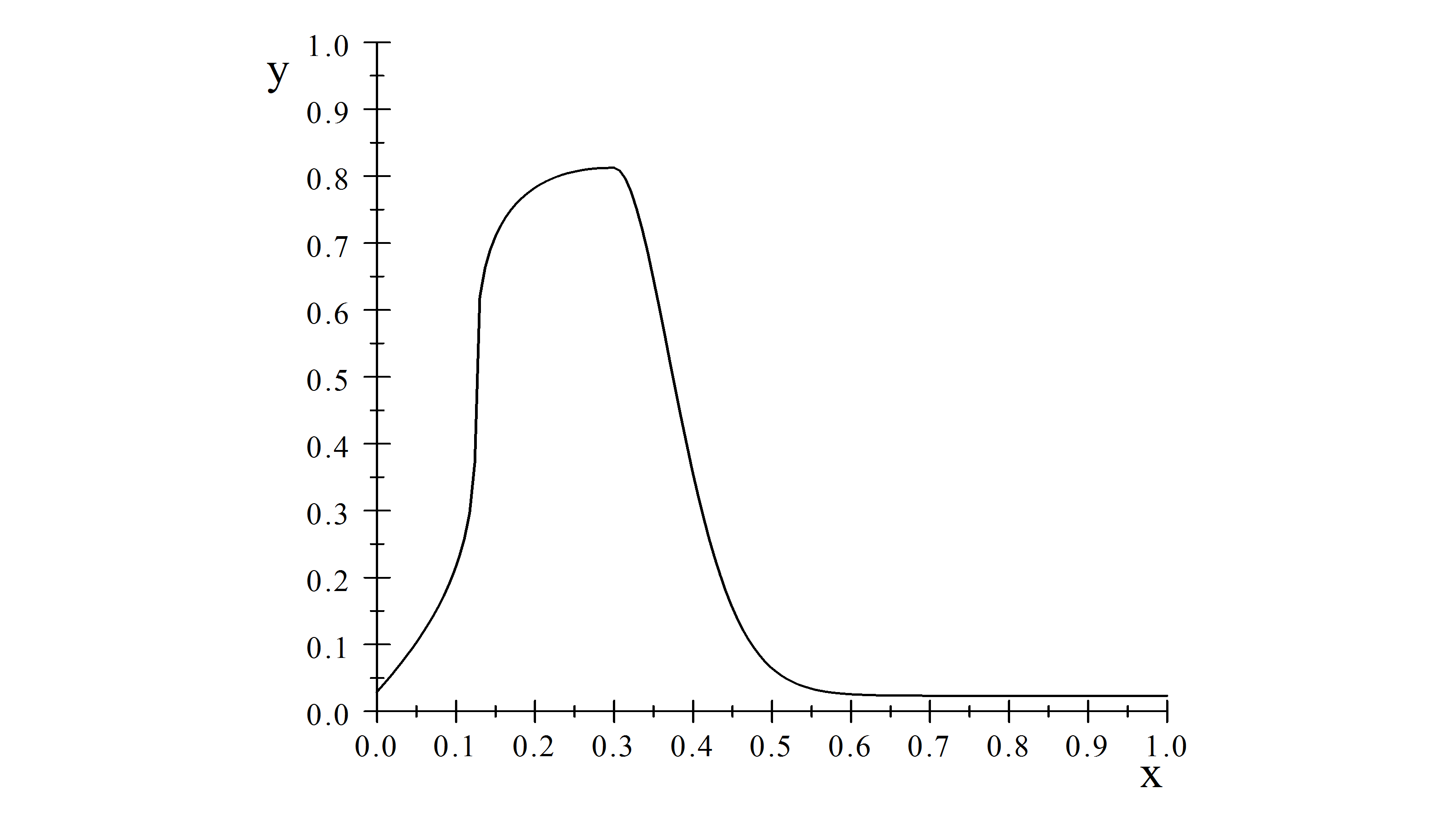
The graph ot the map $T$ is represented in Figure 1. At each iteration of the map a uniformly distributed noise perturbation with span of size $\xi$ is applied, by a kernel $\rho_{0}=\xi^{-1}1_{[-\xi/2,\xi/2]}$, We consider reflecting boundaries when the noise is big enough to send points out of the space $[0,1]$. We remark that this is never the case when the noise amplitude is smaller than the parameter $b$.

In [42] the authors consider several different values for the noise range, showing numerically that there is a transition from positive to negative Lyapunov exponents as the noise range increases. This statement was proved with a computer aided proof in [24]. We now select two different noises amplitudes (one with positive and one with negative Lyapunov exponent) for which the mixing assumption can be proved.

Lemma 48.

Let us consider $\xi_{1}=$ $0.860\times 10^{-2}$ and $\xi_{2}=0.129\times 10^{-3}$ and the kernels $\rho_{i}=\xi_{i}^{-1}1_{[-\xi_{i}/2,\xi_{i}/2]}$  Let us consider the transfer operator $L_{\xi_{i}}:=\rho_{i}\hat{\ast}L_{T}$ associated to these systems satisfy assumption $(LR1)$ of Theorem 3 (mixing).

Proof.

In [24], Table 1 (first and last line) the reader can find a rigorous estimate for the mixing rate of the transfer operator $L_{\xi_{i}}$ related to the size noise $\xi_{i}.$ In particular it is shown that for the noise size $\xi_{1}$   $\|L_{\xi_{1}}^{55}|_{V}\|_{L^{1}}\leq 0.059$  and $\xi_{2}$   $\|L_{\xi_{2}}^{70}|_{V}\|_{L^{1}}\leq 0.41$  proving the exponential contraction of the zero average space in $L^{1}$ and in particular the mixing assumption.    

Note that with those values of the noise, the transfer operator is regularizing from $L^{1}$ to $BV[0,1]$ in the sense of Corollary 22. The above statement also holds for the other noise amplitudes considered in [24], but we will not enter in the details in this paper. Now we focus on a class of perturbations of $T$ such that the derivative operator exist. Let us consider family of perturbations $T_{\delta}=$ $D_{\delta}\circ T$ as in the previous section, such that $D_{\delta}={\mathds{1}}+\delta S$ with $S$ 1-Lipschitz, suppose that the support $\chi_{S}$ of $S$ does not contain a neighborhood of the global maximum $m_{T}$ of $T.$ We see that such a class of perturbations satisfies Proposition 28.

Lemma 49.

Let $T$ be the map defined at $($39$)$. Let us consider $T_{\delta}=$ $D_{\delta}\circ T$, such that $D_{\delta}={\mathds{1}}+\delta S$ and $\chi_{S}$ does not contain a neighborhood of $m_{T}$. Then $L_{T}:BV([0,1])\rightarrow BV(\chi_{S})$ is continuous.

Proof.

This follows from the remark that outside a neighborhood of $m_{T}$ the map is made of a finite set of convex monotone $C^{2}$ branches with derivative bounded away from zero.    

We now have everything we need to apply Theorem 3 (Corollary 33) and get

Proposition 50.

Let us consider the random dynamical system  formed by the map $T$ defined at (39) and uniformly distributed additive noise of radius $\xi_{i}$ as in the statement of Lemma 48.  If we consider a family of systems obtained by the deterministic perturbation of $T$ as described before: $T_{\delta}=$ $D_{\delta}\circ T$, such that $D_{\delta}={\mathds{1}}+\delta S$, $S$ being $1$-Lipschitz and $\chi_{S}$ does not contain a neighborhood of $m_{T}$. Let us consider the associated transfer operators $L_{\xi,T_{\delta}}:=\rho_{\xi}\hat{\ast}L_{D_{\delta}\circ T}.$ Then the system has linear response: let $f_{0}$ be the stationary measure of $L_{\xi,T_{0}}$ and $f_{\delta}$ some stationary measure of $L_{\xi,T_{\delta}},$ then

$$\lim_{\delta\rightarrow 0}\left\|\frac{f_{\delta}-f_{0}}{\delta}-R(1,L_{\xi,T_{0}})[\rho_{\xi}\hat{\ast}(-L_{T}(f_{0})S)^{\prime}]\right\|_{1}=0.$$

5.4. Small random deterministic perturbations of a system with additive noise

In this subsection we consider an example of a family of random systems modeling the following situation: we consider two systems, one is deterministic and the other is random with additive noise. At every iteration we can randomly decide to apply one system or the other. The random system is a random map with additive noise  $x_{n+1}\rightarrow T_{1}(x_{n})+\omega_{n}$ where $T_{1}$ is nonsingular and  $\omega_{n}$ is an i.i.d random variable, as in equation (9), distributed according to a certain $BV$ kernel $\rho$ (with associated transfer operator $L_{0}$ as described in Section 2). We apply this system with probability $(1-\delta).$ The deterministic system is a nonsingular map $T_{2}$ (the transfer operator associated to $T_{2}$ is denoted by $L_{T_{2}}:L^{1}\rightarrow L^{1}$) we apply this second system with probability $\delta$ independent from the previous history of the system. We will also suppose that $T_{2}$ is such that $L_{T_{2}}:BV[0,1]\rightarrow BV[0,1]$ is continuous. When $\delta$ is small we consider this as a small random perturbation of the random system described by $L_{0}$. The (annealed) transfer operator associated to the randomly perturbed system can be defined by

(40) $$L_{\delta}=(1-\delta)L_{0}+\delta L_{T_{2}}.$$

We remark that for $\delta>0$ this operator has not an absolutely continuous kernel; however our theory can still be applied to it provided $L_{0}$ and its perturbation satisfy the assumptions of Theorem 3.  Systems of the type (40) were already studied in [39, Section 10.4], called there “randomly applied stochastic perturbation”, with respect to asymptotic stability (see the reference for the details) but not with respect to linear response. See also the beginning of [39, Section 10.5] for other relevant cases of similar situations and a bit of literature. In this case we have the following situation

Proposition 51.

Let $L_{0}$ and $L_{T_{2}}$ as above, suppose $L_{0}$ satisties Assumption $(LR1)$ of Theorem 3. Let us consider the perturbation $L_{\delta}$ of $L_{0}$ as defined in $(\ref{defino})$. Suppose $L_{\delta}f_{\delta}=f_{\delta}$ for $\delta\in\left[0,\overline{\delta}\right)$. Then the following response formula holds

$$\lim_{\delta\rightarrow 0}\left\|\frac{f_{\delta}-f_{0}}{\delta}-R(1,L_{0})(L_{T_{2}}f_{0}-f_{0})\right\|_{1}=0.$$

Proof.

The statement is a direct application of Theorem 3. Assumption $(LR1)$ is supposed to hold for $L_{0}$. As before, Assumption $(LR2)$ of Theorem 3 is satisfied because of the regularization inequalities proved in Corollary 22. We verify that $\|f_{\delta}\|_{BV}$ is uniformly bounded (assumption $(LR0)$ of Theorem 3). Here we use that $\|L_{T_{2}}\|_{BV\rightarrow BV}$ is bounded. Remark that

$$||L_{\delta}\mu||_{BV}=||(1-\delta)L_{0}\mu||_{BV}+||\delta L_{T_{2}}\mu||_{BV}\leq 9||\rho||_{BV}+\delta||L_{T_{2}}||_{BV\rightarrow BV}||\mu||_{BV}.$$

If $\delta$ is small ehough  $\delta||L_{T_{2}}||_{BV\rightarrow BV}<1$ and this is a kind or Lasota Yorke inequality. Iterating it, we get that eventually for $n$ large enough

$$||L^{n}\mu||_{BV}\leq\frac{2||\rho||_{BV}}{1-\delta||L_{T_{2}}||_{BV\rightarrow BV}}$$

and we can perform the same construction as in Lemma 4. To verify Assumption $(LR3)$ we consider as a weak norm the $L^{1}$ norm itself. To verify the first part of Assumption $(LR3)$ it is sufficient to prove that there is $K>0$ such that

$$\left||L_{0}-L_{\delta}|\right|_{L^{1}\rightarrow L^{1}}\leq K\delta$$

for $\delta$ small enough. This is done by noticing that in our case

$$||L_{0}-L_{\delta}||_{L^{1}\rightarrow L^{1}} = ||\delta L_{T_{2}}-\delta L_{0}||_{L^{1}\rightarrow L^{1}}=\delta||L_{T_{2}}-L_{0}||_{L^{1}\rightarrow L^{1}}$$

$$\leq 2\delta.$$

(the transfer operators are weak contractions in $L^{1}$). To verify the second part of Assumption $(LR3)$ and compute a derivative operator we have to show the convergence in the $L^{1}$ of the limit

$$\underset{\delta\rightarrow 0}{\lim}\frac{(L_{0}-L_{\delta})}{\delta}f_{0}.$$

Again this is very simple because

$$\underset{\delta\rightarrow 0}{\lim}\frac{(L_{0}-L_{\delta})}{\delta}f_{0}=(L_{T_{2}}-L_{0})f_{0}=L_{T_{2}}f_{0}-f_{0}.$$

Applying Theorem 3 we get a linear reponse formula:

(41) $$\lim_{\delta\rightarrow 0}\left\|\frac{f_{\delta}-f_{0}}{\delta}-R(1,L_{0})(L_{T_{2}}f_{0}-f_{0})\right\|_{1}=0.$$

   

6. (Optimal) control of the statistical properties

An important problem related to linear response is the control of the statistical properties of a system: how one can perturb the system, in order to modify its statistical properties in a prescribed way? how can one do it optimally? (what is the best action to be taken in a possible set of allowed small perturbations in order to achieve a given small modification of the stationary measure?).

The understanding of this problem has potentially a great importance in the applications, as it is related to questions about optimal strategies in order to influence the behavior of a system. As an example, thinking about climate models one could ask “what is the best action to be taken in order to reduce the average temperature?” or similarly for other statistical properties. This type of questions is still not much investigated in the literature. In [23] the problem was faced and discussed in general, giving a detailed description of the solutions and the existence of optimal ones in the case of deterministic perturbations of expanding maps. In [34] a similar problem was considered for more general systems, restricting the allowed set of perturbations to conjugacies. In [41] problems of this kind were investigated in connection with the management of complex dynamical systems (networks with many interdependent components). In [6] several related problems, still focusing on optimal perturbations, are investigated for Markov Chains and applied to Ulam approximations of random dynamical systems on the interval.

Let us start formalizing the problem more precisely: suppose we have a system represented by its transfer operator $L_{0}$ and a family of perturbations $L_{\delta,\gamma},$ of magnitude $\delta$ and direction $\gamma\in D$ varying in a set $D$ of the allowed “infinitesimal” perturbations. Suppose $f_{0}$ is a stationary measure of $L_{0}$ and $f_{\delta,\gamma}$ is a stationary measure of $L_{\delta,\gamma}$

1. can we find a perturbation $\gamma\in D,$ leading to some wanted direction of change of the stationary measure? (in the sense of prescribed linear response $\mu$).

2. In case of many solutions in $D$, can we find an optimal one?

3. In case of no solutions in $D$, can we find an optimal perturbation in $D$, approximating as well as possible the wanted response?

Formally the request problem $1)$ translates into the following: given $\mu,$ find $\gamma$ such that

$$\lim_{\delta\rightarrow 0}\frac{f_{\delta,\gamma}-f_{0}}{\delta}=\mu.$$

The limit above can be considered in different topologies, in this paper we considered the $L^{1}$ and the $W$ topology, but other topologies could be considered, including the convergence under different observables: i.e. suppose $\psi$ is a smooth observable with values in $\mathbb{R}^{n}$, one may consider the problem of finding $\gamma$ for which it holds

$$\lim_{\delta\rightarrow 0}\frac{\int\psi~{}df_{\delta,\gamma}-\int\psi~{}df_{0}}{\delta}=\int\psi~{}d\mu$$

in $\mathbb{R}^{n}$. Formalizations of problems $2)$ and $3)$ can be made similarly, using linear response. Similar questions may consider the maximum response in some norm or the one of a given observable in some norm (see [6]).

Having obtained in the previous section handy and explicit results for the linear response of systems with additive noise, we now consider problem $1)$ and discuss briefly its mathematical structure. As done in the previous sections, let us allow perturbations of the deterministic part of the system of the form $T_{\delta}=({\mathds{1}}+\delta S)\circ T$, with $S$ being $1$-Lipschitz and let us consider as perturbed operators $L_{\delta,\gamma}$ the associated transfer operators $L_{\delta,S}:=\rho_{\xi}\ast L_{({\mathds{1}}+\delta S)\circ T}.$ Consider the linear response formula  found before for these kind of perturbations: let $f_{0}$ be the stationary measure of $L_{0,S}$ and $f_{\delta}$ some stationary measure of $L_{\delta,S},$ then under the assumptions of Theorem 3 and Proposition 14 we have the linear response formula,

$$\lim_{\delta\rightarrow 0}\frac{f_{\delta}-f_{0}}{\delta}=R(1,L_{\xi,T_{0}})[\rho_{\xi}\hat{\ast}(-L_{T_{0}}(f_{0})S)^{\prime}]=\mu$$

(with convergence in $L^{1}$). This equation in now to be solved for $S$. Leading to

$$\rho_{\xi}\hat{\ast}(-L_{T_{0}}(f_{0})S)^{\prime}=\mu{-}L_{\xi,T_{0}}\mu.$$

Now denote by $N_{\xi}:L^{1}\rightarrow BV$ the convolution operator: $N_{\xi}(f)=\rho_{\xi}\hat{\ast}f$ . $N_{\xi}$ is not necessarily injective or onto (it is not injective due to the boundary arrangements, but in the case of the map defined at $($39$)$ it is when the noise is small enough because the image of the map is strictly contained in $[0,1]$). Suppose $\mu{-}L_{\xi,T_{0}}\mu$ is in the range of $N_{\xi}$ and denote by

$$N_{\xi}^{-1}(g)=\{f\in L^{1}~{}s.t.N_{\xi}(f)=g\}.$$

We have

$$(-L_{T}(f_{0})S)^{\prime}\in N_{\xi}^{-1}(\mu{-}L_{\xi,T_{0}}\mu)$$

leading to the explicit family of solutions to the control problem $1)$

$$S(t)=\frac{C+\int_{0}^{t}f~{}dm}{-L_{T_{0}}(f_{0})}$$

for every $C\in\mathbb{R}$ and $f\in N_{\xi}^{-1}(\mu{-}L_{\xi,T_{0}}\mu)$ when the expression makes sense. Inside this family one can search for optimal or optimal approximating solutions, as proposed at problems $2)$ and $3)$ above. Further investigations of these problems are in our opinion very interesting, but out of the scope of the present paper.

Remark 52.

Note that, analogously to what has been done before in remark 31, we can compare this result with the one in [23]. Over there the solution to the problem is computed, given $\rho_{1}$ by the solution of a differential equation which is, morally, what has been done here.

References

- [1] Abramov, Rafail V. Leading order response of statistical averages of a dynamical system to small stochastic perturbations. J. Stat. Phys. 166 (2017), no. 6, 1483–1508.
- [2] Alves, J. F. and Carvalho, M. and Freitas, J.M. Statistical stability and continuity of SRB entropy for systems with Gibbs-Markov structures, Communications in Mathematical Physics, 296, 2010 , 739–767, doi: 10.1007/s00220-010-1027-6
- [3] J. F. Alves, M. Soufi Statistical Stability in Chaotic Dynamics Progress and Challenges in Dyn. Sys. Springer Proc. in Math. & Statistics V. 54, 2013, pp 7-24
- [4] Alves J. F. and Viana, M. Statistical stability for robust classes of maps with non-uniform expansion, Ergodic Theory and Dynamical Systems, 22 ,2002 , doi: 10.1017/S0143385702000019
- [5] Arnold L., Random Dynamical Systems Springer Monographs in Mathematics Springer (Berlin,2003)
- [6] F. Anton D. Dragicevic G. Froyland Optimal linear responses for Markov chains and stochastically perturbed dynamical sistems J. Stat. Phys., 170, Issue 6, pp 1051–1087 ( 2018).
- [7] W. Bahsoun, S Galatolo, I. Nisoli, X. Niu A Rigorous Computational Approach to Linear Response Nonlinearity 31 (2018), no. 3, 1073–1109
- [8] W. Bahsoun, M. Ruziboev, B. Saussol Linear response for random dynamical systems arXiv:1710.03706
- [9] Bahsoun, W., Saussol, B., Linear response in the intermittent family: differentiation in a weighted -norm, Discrete Contin. Dyn. Syst. 36 (12) (2016) pp. 6657-6668
- [10] Baladi, V., On the susceptibility function of piecewise expanding interval maps, Comm. Math. Phys. 275 (3) (2007) pp. 839-859
- [11] Baladi, V., Smania, D., Linear response formula for piecewise expanding unimodal maps, Nonlinearity 21 (4) (2008) pp. 677-711
- [12] Baladi, V., Todd, M., Linear response for intermittent maps, Comm. Math. Phys. 347 (3) (2016), pp. 857-874
- [13] V. Baladi Linear response, or else Proceedings of the International Congress of Mathematicians—Seoul 2014. Vol. III, (2014) pp. 525–545
- [14] V. Baladi , M. Benedicks , N. Schnellmann Whitney-Holder continuity of the SRB measure for transversal families of smooth unimodal maps Invent. Math. 201 773-844 (2015)
- [15] V. Baladi, T. Kuna and V. Lucarini Linear and fractional response for the SRB measure of smooth hyperbolic attractors and discontinuous observables Nonlinearity 30 1204-1220 (2017)
- [16] R. Bhattacharya, M. Majumdar, Random Dynamical Systems: Theory and Applications Cambridge University Press (2007)
- [17] MD Chekroun, E Simonnet, M Ghil Stochastic climate dynamics: Random attractors and time-dependent invariant measures Physica D: Nonlinear Phenomena, 2011
- [18] Dolgopyat, D., On differentiability of SRB states for partially hyperbolic systems, Invent. Math. 155 (2) (2004) pp. 389-449
- [19] Dolgopyat, D. Prelude to a kiss. Modern dynamical systems and applications, 313–324, Cambridge Univ. Press, Cambridge, 2004.
- [20] Galatolo, S. Statistical properties of dynamics. Introduction to the functional analytic approach, arXiv:1510.02615
- [21] S. Galatolo Quantitative statistical stability and convergence to equilibrium. An application to maps with indifferent fixed points Chaos, Solitons & Fractals V. 103, pp. 596-601 (2017).
- [22] S. Galatolo Quantitative statistical stability and speed of convergence to equilibrium for partially hyperbolic skew products J. Éc. polytech. Math. 5 (2018), 377–405.
- [23] Galatolo S., Pollicott M, Controlling the statistical properties of expanding maps, Nonlinearity 30 (2017) pp. 2737-2751
- [24] S. Galatolo, M. Monge, I. Nisoli Existence of Noise Induced Order, a Computer Aided Proof arXiv:1702.07024
- [25] P. Giulietti, A.O. Lopes, D. Marcon and B. Kloeckner, The Calculus of Thermodynamic Formalism, Journal of the European Mathematical Society, 20 (2018), doi:10.4171/JEMS/814
- [26] M. Ghil The wind-driven ocean circulation: applying dynamical system theory to a climate problem. Disc. Cont. Dyn. Sys. V. 37, N. 1, (2017).
- [27] C. Gonzalez-Tokman Multiplicative ergodic theorems for transfer operators: towards the identification and analysis of coherent structures in non-autonomous dynamical systems https://people.smp.uq.edu.au/CeciliaTokman/ , Contemporary Mathematics to appear (2018).
- [28] P. Gora Invariant densities for piecewiser linear maps of the unit interval Ergodic Theory and Dynamical systems, 20, 1-10 (2008)
- [29] P. Gora , A. Boyarsky Laws of chaos - Invariant measures and dynamical systems in one dimension Spriger (1997)
- [30] M Hairer, AJ Majda A simple framework to justify linear response theory Nonlinearity 23 (2010) 909–922
- [31] Keller, Gerhard Stochastic stability in some chaotic dynamical systems, Monatshefte für Mathematik, 94, 1982, 313–333, doi:10.1007/BF01667385
- [32] G. Keller, C. Liverani Stability of the spectrum for transfer operators Ann. Scuola Norm. Sup. Pisa Cl. Sci. (4) 28 no. 1, 141-152 (1999).
- [33] Kifer, Yuri Random perturbations of dynamical systems, Progress in Probability and Statistics, 16, Birkhäuser Boston, Inc., Boston, MA, 1988, ISBN:0-8176-3384-7, doi:10.1007/978-1-4615-8181-9
- [34] B. R. Kloeckner The linear request problem Proc. Amer. Math. Soc. 146 (2018), no. 7, 2953–2962.
- [35] B. R. Kloeckner and A. O. Lopes and M. Stadlbauer, Contraction in the Wasserstein metric for some Markov chains, and applications to the dynamics of expanding maps. Nonlinearity vol. 28-11 (2015), doi:10.1088/0951-7715/28/11/4117
- [36] Kopf, C. Invariant measures for piecewise linear transformations of the interval Applied Mathematics and computation vol. 39, 123-144 (1990)
- [37] Korepanov, A. Linear response for intermittent maps with summable and nonsummable decay of correlations, Nonlinearity 29 (6) (2016) pp. 1735-1754
- [38] Lasota, A.; Mackey, M. C., Probabilistic Properties of Deterministic Systems. Cambridge University Press 1986.
- [39] Lasota, A. ; Mackey, Michael C. Chaos, fractals, and noise, Applied Mathematical Sciences, 97 2nd Ed. Springer-Verlag, 1994, doi:10.1007/978-1-4612-4286-4
- [40] J. A. Freund, T. Poschel (Eds.), “Stochastic Processes in Physics, Chemistry, and Biology”, Lecture Notes in Physics 557 (2000), Springer, Berlin.
- [41] MacKay R. S. Management of complex dynamical systems Nonlinearity V. 31, N. 2 (2018)
- [42] Matsumoto K., Tsuda I. Noise-induced Order J. Stat. Phys Vol. 31, No. 1, pp. 87-106 (1983)
- [43] Majda, A.J. Challenges in climate science and contemporary applied mathematics Comm. Pure Appl. Math. Volume 65, Issue 7 pp. 920–948 (2012)
- [44] Mazzolena, M. Dinamiche espansive unidimensionali: dipendenza della misura invariante da un parametro Master Thesys, Department of Mathematics, University of Rome Tor Vergata
- [45] Mitrophanov, A. Yu. Sensitivity and convergence of uniformly ergodic Markov chains. J. Appl. Probab. 42 (2005), no. 4, 1003–1014.
- [46] Liverani, C. Invariant measures and their properties. A functional analytic point of view. Dynamical systems. Part II, pp. 185-237, Pubbl. Cent. Ric. Mat. Ennio Giorgi, Scuola Norm. Sup., Pisa, 2003
- [47] V. Lucarini Stochastic Perturbations to Dynamical Systems: A Response Theory Approach Journal of Statistical Physics 2012, Volume 146, Issue 4, pp 774–786
- [48] Lucarini, V., Blender, R., Herbert, C., Pascale, S., Wouters, J., Mathematical and Physical Ideas for Climate Science, Rev. Geophys. 52 (2014), pp. 809–859
- [49] M. Pollicott, P. Vytnova, Linear response and periodic points. Nonlinearity 29 (2016), no. 10, 3047–3066.
- [50] W. Rudin Fourier Analysis on groups Interscience publishers. (1962)
- [51] Ruelle, D., Differentiation of SRB states, Comm. Math. Phys. 187 (1997) pp. 227-241
- [52] J. Sedro A regularity result for fixed points, with applications to linear response arXiv:1705.04078
- [53] Viana M. Stochastic dynamics of deterministic systems IMPA (1997) http://w3.impa.br/~viana/out/sdds.pdf
- [54] Viana M. Lectures on Lyapunov Exponents, Cambridge Studies in Advanced Mathematics 145, Cambridge University Press (2014)
- [55] Z. Zhang On the smooth dependence of SRB measures for partially hyperbolic systems arXiv:1701.05253