Nearby Early-Type Galactic Nuclei at High Resolution – Dynamical Black Hole and Nuclear Star Cluster Mass Measurements

Abstract

We present a detailed study of the nuclear star clusters (NSCs) and massive black holes (BHs) of four of the nearest low-mass early-type galaxies: M32, NGC 205, NGC 5102, and NGC 5206. We measure dynamical masses of both the BHs and NSCs in these galaxies using Gemini/NIFS or VLT/SINFONI stellar kinematics, Hubble Space Telescope (HST) imaging, and Jeans Anisotropic Models. We detect massive BHs in M32, NGC 5102, and NGC 5206, while in NGC 205, we find only an upper limit. These BH mass estimates are consistent with previous measurements in M32 and NGC 205, while those in NGC 5102 & NGC 5206 are estimated for the first time, and both found to be $<$$10^{6}$$M_{\odot}$. This adds to just a handful of galaxies with dynamically measured sub-million $M_{\odot}$ central BHs. Combining these BH detections with our recent work on NGC 404’s BH, we find that 80% (4/5) of nearby, low-mass ($10^{9}-10^{10}$$M_{\odot}$; $\sigma_{\star}\sim 20-70$ km s^-1) early-type galaxies host BHs. Such a high occupation fraction suggests the BH seeds formed in the early epoch of cosmic assembly likely resulted in abundant seeds, favoring a low-mass seed mechanism of the remnants, most likely from the first generation of massive stars. We find dynamical masses of the NSCs ranging from $2-73\times 10^{6}$$M_{\odot}$ and compare these masses to scaling relations for NSCs based primarily on photometric mass estimates. Color gradients suggest younger stellar populations lie at the centers of the NSCs in three of the four galaxies (NGC 205, NGC 5102, and NGC 5206), while the morphology of two are complex and are best-fit with multiple morphological components (NGC 5102 and NGC 5206). The NSC kinematics show they are rotating, especially in M32 and NGC 5102 ($V/\sigma_{\star}\sim 0.7$).

1. Introduction

Supermassive black holes (SMBHs) appear to be ubiquitous features of the centers of massive galaxies. This is inferred in nearby galaxies, both from their dynamical detection (see review by Kormendy & Ho, 2013), and from the presence of accretion signatures (e.g., Ho et al., 2009). Furthermore, the mass density of these BHs in nearby massive galaxies is compatible with the inferred mass accretion of active galactic nuclei (AGN) in the distant universe (e.g., Marconi et al., 2004). However, the presence of central BHs is not well constrained in lower mass galaxies, particularly below stellar masses of $\sim$10¹⁰ $M_{\odot}$ (e.g., Greene, 2012; Miller et al., 2015). These lower mass galaxy nuclei are almost universally populated by bright, compact nuclear star clusters (NSCs) (e.g., Georgiev & Böker, 2014; den Brok et al., 2014b) with half-light/effective radius of $r_{\rm eff}\sim 3$ pc. These NSCs are known to co-exist in some cases with massive BHs, including in the Milky Way (MW Seth et al., 2008; Graham & Spitler, 2009; Neumayer & Walcher, 2012).

Finding and weighing central BHs in lower mass galaxies is challenging due to the difficulty of dynamically detecting the low-mass ($\lesssim$$10^{6}$$M_{\odot}$) BHs they host. However, it is a key measurement for addressing several related science topics. First, low-mass galaxies are abundant (e.g., Blanton et al., 2005), and thus if they commonly host BHs, these will dominate the number density (but not mass density) of BHs in the local universe. This has consequences for a wide range of studies, from the expected rate of tidal disruptions (Kochanek, 2016), to the number of BHs we expect to find in stripped galaxy nuclei (e.g., Pfeffer et al., 2014; Ahn et al., 2017). Second, the number of low-mass galaxies with central BHs is currently most feasible way to probe the unknown formation mechanism of massive BHs. More specifically, if massive BHs form from the direct collapse of relatively massive $\sim$10⁵$M_{\odot}$ seed black holes scenario (e.g., Lodato & Natarajan, 2006; Bonoli et al., 2014), few would be expected to inhabit low-mass galaxies, if, on the other hand, they form from the remnants of Population III stars, a much higher “occupation fraction” is expected in low-mass galaxies (Volonteri et al., 2008; van Wassenhove et al., 2010; Volonteri, 2010). This work is complementary to work that is starting to be undertaken at higher redshifts to probe accreting black holes at the earliest epochs (e.g., Weigel et al., 2015; Natarajan et al., 2017; Volonteri et al., 2017). Tidal disruptions are also starting to probe the BH population of low mass galaxies (e.g., Wevers et al., 2017; Law-Smith et al., 2017), and may eventually provide constraints on occupation fraction (e.g., Stone & Metzger, 2016). Third, dynamical mass measurements of SMBHs ($M_{\rm SMBH}$ $\sim 10^{6}-10^{10}$$M_{\odot}$) have shown that their masses scale with the properties of their host galaxies such as their bulge luminosity, bulge mass, and velocity dispersion (Kormendy & Ho, 2013; McConnell & Ma, 2013; Graham & Scott, 2015; Saglia et al., 2016). These scaling relations have been used to suggest that galaxies and their central SMBHs coevolve, likely due to feedback from the AGN radiation onto the surrounding gas (see review by Fabian, 2012).

The black hole–galaxy relations are especially tight for massive early-type galaxies (ETGs), while later-type, lower dispersion galaxies show a much larger scatter (Greene et al., 2016; Läsker et al., 2016b). However, the lack of measurements at the low-mass, low-dispersion end, especially in ETGs means that our knowledge of how BHs populate host galaxies is very incomplete.

The population of known BHs in low-mass galaxies was recently compiled by Reines & Volonteri (2015). Of the BHs known in galaxies with stellar masses $<$10¹⁰$M_{\odot}$, most have been found by the detection of optical broad-line emission, with their masses inferred from the velocity widths of their broad-lines (e.g., Greene & Ho, 2007; Dong et al., 2012; Reines et al., 2013). Many of these galaxies host BHs with inferred masses below 10⁶$M_{\odot}$, especially those with stellar mass $\lesssim$$3\times 10^{9}$$M_{\odot}$. Broad-line emission is however found in only a tiny fraction ($<$1%) of low-mass galaxies; other accretion signatures that are also useful for identifying BHs in low-mass galaxies include narrow-line emission (e.g., Moran et al., 2014), coronal emission in the mid-infrared (e.g., Satyapal et al., 2009), tidal-disruption events (e.g., Maksym et al., 2013), and hard X-ray emission (e.g., Miller et al., 2015; She et al., 2017).

The current record holder for the lowest mass central BH in a late-type galaxy (LTG) is the broad-line AGN in RGG 118 with $M_{\star}\sim 2\times 10^{9}$ $M_{\odot}$ ($M_{\rm BH}$ = $5\times 10^{4}$$M_{\odot}$; Baldassare et al., 2015). The lowest-mass systems known to host central massive BHs are ultracompact dwarfs, which are likely stripped galaxy nuclei (Seth et al., 2014; Ahn et al., 2017). Apart from these systems, the lowest mass BH-hosting galaxies are the $M_{\star}\sim 3\times 10^{8}$ $M_{\odot}$ early-type dwarf in Abell 1795, where a central BH is suggested by the detection of a tidal-disruption event (Maksym et al., 2013), and the similar mass dwarf elliptical galaxy Pox 52, which hosts a broad-line AGN (Barth et al., 2004; Thornton et al., 2008). Currently, there are only a few galaxies with sub-million solar mass dynamical BH mass estimates, including NGC 4395 ($M_{\rm BH}$ = $4^{+8}_{-3}\times 10^{5}$$M_{\odot}$; den Brok et al., 2015), NGC 404 ($M_{\rm BH}$ $\lesssim 1.5\times 10^{5}$$M_{\odot}$; Nguyen et al., 2017), and NGC 4414 ($M_{\rm BH}$ $\lesssim 1.6\times 10^{6}$$M_{\odot}$; Thater et al., 2017).

Unlike BHs, the morphologies, stellar populations, and kinematics of NSCs provide an observable record for understanding mass accretion into the central parsecs of galaxies. The NSCs’ stellar mass accretion can be due to (1) the migration of massive star clusters formed at larger radii that then fall into the galactic center via dynamical friction (e.g., Lotz et al., 2001; Antonini, 2013; Guillard et al., 2016) or (2) the in-situ formation of stars from gas that falls into the nucleus (e.g., Seth et al., 2006; Antonini et al., 2015b). Observations suggest the formation of NSCs is ongoing, as they typically have multiple populations (e.g., Rossa et al., 2006; Nguyen et al., 2017). Most studies on NSCs in ETGs have focused on galaxies in nearby galaxy clusters (Walcher et al., 2006); spectroscopic and photometric studies suggest that typically the NSCs in these ETGs are younger than their surrounding galaxy, especially in galaxies $\lesssim 2\times 10^{9}$ M_⊙ (e.g., Côté et al., 2006; Paudel et al., 2011; Krajnović et al., 2017; Spengler et al., 2017). There is also a clear change in the scaling relations between NSC and galaxy luminosities and masses at about this mass, with the scaling being shallower at lower masses and steeper at higher masses (Scott et al., 2013; den Brok et al., 2014b; Spengler et al., 2017). This change in addition to the flattening of more luminous NSCs (Spengler et al., 2017) suggests a possible change in the formation mechanism of NSCs from migration to in-situ formation. However, the NSC scaling relations for ETGs are based almost entirely of photometric estimates, with a significant sample of dynamical measurements available only for nearby late-type spirals (Walcher et al., 2005) and only two in ETG FCC 277 (Lyubenova et al., 2013) and NGC 404 (Nguyen et al., 2017).

The relationship between NSCs and BHs is not well understood. The sample of objects with both a detected NSC and BH is quite limited (Seth et al., 2008; Graham & Spitler, 2009; Neumayer & Walcher, 2012; Georgiev et al., 2016), but even from this data it is clear that low-mass galaxy nuclei are typically dominated by NSCs, while high mass galaxy nuclei are dominated by SMBHs. This transition could be due to a number of mechanisms, including the tidal disruption of infalling clusters (Ferrarese et al., 2006; Antonini et al., 2015a), the growth of BH seeds in more massive galaxies by tidal disruption of stars (Stone et al., 2017), or differences in feedback from star formation vs. AGN accretion (Nayakshin et al., 2009). In addition, the formation of NSCs and BHs could be explicitly linked with NSCs creating the needed initial seed BHs during formation (e.g., Portegies Zwart et al., 2004), or strong gas inflow creating the NSC and BH simultaneously (Hopkins & Quataert, 2010). However, the existence of a BH around which a NSC appears to be currently forming in the nearby galaxy Henize 2-10 suggests that BHs can form independently of NSCs (Nguyen et al., 2014).

This work presents a dynamical study of the BHs and NSCs of four nearby low-mass ETGs including the two brightest companions of Andromeda, M32 and NGC 205, and two companions of Cen A, NGC 5102 and NGC 5206. Of these four galaxies, previous BH mass estimates exist for two; the detection of $(2.5\pm 0.5)\times 10^{6}$$M_{\odot}$ BH in M32 (Verolme et al., 2002; van den Bosch & de Zeeuw, 2010), and the upper limit of $3.8\times$$10^{4}$$M_{\odot}$ (at 3$\sigma$) in NGC 205 (Valluri et al., 2005). In this paper, we use adaptive optics integral field spectroscopic measurements, combined with dynamical modeling using carefully constructed mass models to constrain the BH and NSC masses in all four galaxies, including the first published constraints on the BHs of NGC 5102 and NGC 5206.

This paper is organized into nine sections. In Section 2, we describe the observations and data reduction. The four galaxies’ properties are presented in Section 3, and we construct luminosity and mass models in Section 4. We present kinematics measurements of their nuclei in Section 5. We model these kinematics using Jeans models and present the BH constraints and uncertainties in Section 6. In section 7 we analyze the properties of the NSCs and present our measurements of their masses. We discuss our results in Section 8, and conclude in Section 9.

2. Data and Data Reduction

2.1. HST Imaging

The HST/WFPC2 PC and ACS/HRC imaging we use in this work is summarized in Table 1. The nuclei of M32 and NGC 5206 are observed in the WFPC2 PC chip in F555W and F814W filters. For NGC 205, we use the central ACS/HRC F555W and F814W images. For NGC 5102, we use more imaging of WFPC2 including two central saturated F450W and F560W, unsaturated F547M, and H$\alpha$ emission F656N.

Table 1HST/WFPC2 PC/WF3 and ACS HRC Imaging

Object	$\alpha$(J2000)	$\delta$(J2000)	Camera	Aperture	UT Date	PID	Filter	Exptime	Pixelscale	Zeropoint	A${}_{\rm\lambda}\tablenotemark{b}$
	(h m s)	(∘ $\arcmin$ $\arcsec$)						(s)	($\arcsec$/pix)	(mag)	(mag)
(1)	(2)	(3)	(4)	(5)	(6)	(7)	(8)	(9)	(10)	(11)	(12)
M32	00:42:38.37	40:51:49.3	WFPC2	PC1-FIX	1994 Dec 26	5236	F555W	$4\times 24$	0.0445	24.664	0.047
			WFPC2	PC1-FIX	1994 Dec 26	5236	F814W	$4\times 24$	0.0445	23.758	0.026
NGC 205	00:40:22.0	41:41:07.1	ACS/HRC	HRC	2002 Sep 08	9448	F555W	$4\times 640$	0.0300	25.262	0.047
			ACS/HRC	HRC	2002 Sep 08	9448	F814W	$8\times 305$	0.0300	24.861	0.026
NGC 5102	13:21:55.96	-36:38:13.0	WFPC2	PC1-FIX	1994 Sep 02	5400	F547M	$8\times 70$	0.0445	23.781	0.050
			WFPC2	PC1-FIX	1994 Sep 02	5400	F450W⋆	$11\times 590$	0.0445	24.106	0.058
			WFPC2	PC1-FIX	1994 Sep 02	5400	F569W⋆	$11\times 590$	0.0445	24.460	0.043
			WFPC2	PC1-FIX	2001 May 27	8591	F656N	$5\times 340$	0.0445	19.683	0.035
NGC 5206	13:33:43.92	-48:09:05.0	WFPC2	PC1-FIX	1996 May 11	6814	F555W	$6\times 350$	0.0445	24.664	0.047
			WFPC2	PC1-FIX	1996 May 11	6814	F814W	$6\times 295$	0.0445	23.758	0.026

For the ACS/HRC data we downloaded reduced, drizzled images from the HST/Hubble Legacy Archive (HLA). However, because the HLA images of the WFPC2 PC chip have a pixel-scale that is downgraded by 10%, we re-reduce images, which are downloaded from the Mikulski Archive for Space Telescope (MAST), using Astrodrizzle (Avila et al., 2012) to a final pixel scale of 0$\farcs$0445. For all images, we constrain the sky background by comparing them to ground-based data (see Section 4.1).

We use the centroid positions of the nuclei to align images from all HST filters to the F814W (in M32, NGC 205, and NGC 5206) or F547M (in NGC 5102) data. The astrometric alignment of the Gemini/NIFS or VLT/SINFONI spectroscopic data (Section 2.2) was then also tied to the same images, providing a common reference frame for all images used in this study.

2.2. Integral-Field Spectroscopic Data

2.2.1 Gemini/NIFS Spectroscopy

M32 and NGC 205 were observed with Gemini/NIFS using the Altair tip-tilt laser guide star system. The M32 data were previously presented in Seth (2010). The observational information can be found in Table 2. We use these data to derive stellar kinematics from the CO band-head absorption in Section 5.

The data were reduced using the IRAF pipeline modified to propagate the error spectrum, for details see Seth et al. (2010). The telluric calibration was done with A0V stars, for M32, HIP 116449 was used (Seth, 2010), while for NGC 205 we use HIP 52877. The final cubes were constructed via a combination of six (M32) and eight (NGC 205) dithered on-source cubes with good image quality after subtracting offset sky exposures. The wavelength calibration used both an arc lamp image and the skylines in the science exposures with an absolute error of $\sim$2 km s^-1.

Table 2Gemini/NIFS and VLT/SINFONI Spectroscopic Data

Object	Instrument	UT Date	Mode/	Exptime	Sky	Pixel Scale	$\overline{\rm FWHM}$	$\overline{\rm FWHM}$	PID
			Telescope	(s)		($\arcsec$/pix)	(Å)	(km s-1)
(1)	(2)	(3)	(4)	(5)	(6)	(7)	(8)	(9)	(10)
M32	NIFS	2005 Oct 23	AO + NGS	$6\times 600$	$5\times 600$	0.05	4.2	57.0	GN-2005B-SV-121
NGC 205	NIFS	2008 Sep 19	AO + LGS	$8\times 760$	$6\times 760$	0.05	4.2	55.7	GN-2008B-Q-74
NGC 5102	SINFONI	2007 Mar 21	UT4-Yepun	$12\times 600$	$12\times 600$	0.05	6.2	82.2	078.B-0103(A)
NGC 5206	SINFONI	2011 Apr 28	UT4-Yepun	$3\times 600$	$3\times 600$	0.05	6.2	82.2	086.B-0651(B)
NGC 5206	SINFONI	2013 Jun 18	UT4-Yepun	$3\times 600$	$3\times 600$	0.05	6.2	82.2	091.B-0685(A)
NGC 5206	SINFONI	2014 Mar 22	UT4-Yepun	$3\times 600$	$3\times 600$	0.05	6.2	82.2	091.B-0685(A)

Table 3Gemini/NIFS and VLT/SINFONI PSF models

Object	Observation	Gaussian 1	Gaussian 2	Moffat
		($\arcsec$/frac.)	($\arcsec$/frac.)	($\arcsec$/frac.)
(1)	(2)	(3)	(4)	(5)
M32	NIFS	0.250/45%	…	0.85/55%
NGC 205	NIFS	0.093/68%	…	0.92/32%
NGC 5102	SINFONI	0.079/35%	0.824/65%	…
NGC 5206	SINFONI	0.117/60%	0.422/40%	…
		0.110/53%	0.487/47%	…

2.2.2 VLT/SINFONI Spectroscopy

NGC 5102 and NGC 5206 were observed with SINFONI (Eisenhauer et al., 2003; Bonnet et al., 2004) on the UT4 (Yepun) of the European Southern Observatory’s Very Large Telescope (ESO VLT) at Cerro Paranal, Chile. NGC 5102 was observed in two consecutive nights in March 2007 as part of the SINFONI GTO program (PI: Bender). A total of 12 on-source exposures of 600s integration time were observed in the two nights using the 100 mas pixel scale. NGC 5206 was observed in service mode in three different years (2011, 2013, and 2014; PI: Neumayer) with three on-source exposures of 600s in each of the runs. Both of the targets were observed using the laser guide star for the adaptive optics correction and used the NSC itself for the tip-tilt correction. The spectra were taken in $K$–band (1.93–2.47$\mu$m) at a spectral resolution of R $\sim$ 4000, covering a field of view of $3\arcsec\times 3\arcsec$. The data were reduced using the ESO SINFONI data reduction pipeline, following the steps (1) sky-subtraction, (2) flat-fielding, (3) bad pixel correction, (4) distortion correction, (5) wavelength calibration, (6) cube reconstruction, and finally (8) telluric correction. Details on these steps are given in Neumayer et al. (2007). The final data cubes were constructed via a combination of the individual dithered cubes. This leads to a total exposure time of 7200s for NGC 5102 and 5400s for NGC 5206.

2.3. Point-Spread Function Determinations

Our analysis requires careful characterization of the point-spread functions (PSFs) in both our kinematic and imaging data. The HST PSFs are used in fitting the two-dimensional (2D) surface brightness profiles of the galaxies (GALFIT; Peng et al., 2010), while the Gemini/NIFS and VLT/SINFONI PSFs are used for the dynamical modeling.

For the HST PSFs, we create the model PSF for each HST exposure using the Tiny Tim routine for each involved individual filter for each object. The PSFs are created using the $\tt{tiny1}$ and $\tt{tiny2}$ tasks (Krist, 1995; Krist et al., 2011). We next insert these into corresponding c0m (M32, NGC 5102, and NGC 5206) or flt (NGC 205) images at the positions of the nucleus in each individual exposure to simulate our observations and use Astrodrizzle to create our final PSF as described in den Brok et al. (2015) and Nguyen et al. (2017).

For the PSFs of our integral field spectra, we convolve the HST images with an additional broadening to determine the two component PSF expected from adaptive optics observations. The Gemini/NIFS PSFs for M32 and NGC 205 are estimated as described in Seth et al. (2010). First, the outer shape of the PSF was constrained using images of the telluric calibrator Moffat profile ($\Sigma(r)=\Sigma_{0}/[(1+(r/r_{d})^{2})]^{4.765}$). We then convolved the HST images with a inner Gaussian $+$ outer Moffat function (with fixed shape but free amplitude) to best match the shape of the NIFS continuum image; we refer to these as G + M PSFs. The full widths at half maximum (FWHM) and light fractions of components are presented in Table 3.

The VLT/SINFONI data cubes of NGC 5102 and NGC 5206 contain an apparent scattered light component that affects our data in two ways (1) it creates a structured non-stellar background in the spectra which we subtract off before measuring kinematics, and (2) it is uniform across the field and therefore creates a flat outer profile that cannot be explained with a reasonable PSF. Because this scattered light does not contribute to our kinematic measurements, we do our best to remove this before fitting the PSF. Unfortunately, this component is degenerate with the true PSF. To measure the level of this scattered light, we compare the surface brightness of the SINFONI data to a scaled version of the HST. Because the level of the background in the SINFONI continuum image is much larger than the expected background, we simply subtract of the difference to the HST background before fitting our PSFs. However, as this likely results in somewhat of an oversubtraction, we also create an additional PSF where just half the original value was subtracted off the SINFONI data. This had a negligible effect on the PSF of NGC 5102, however it was more significant for NGC 5206 ($\Delta{\rm FWHM}\sim 18$%). We will discuss the impact of this PSF uncertainty on our dynamical modeling in Section 6.2.2. For the functional form of these PSF, we test several functions and find that the best-fit PSFs are double-Gaussians (2G); their FWHMs and light fractions are presented in Table 3. We note that this is different from the NIFS PSF, which we found was better characterized by a Gauss+Moffat function for M32 and NGC 205.

3. Galaxies Sample Properties

Our sample of galaxies was chosen from known nucleated galaxies within 3.5 Mpc. We look at the completeness of this sample by examining the number of ETGs (numerical Hubble T $\leq 0$) with total stellar masses between $5\times 10^{8}$$M_{\odot}$ $\leq~{}M_{\star}\leq 1\times 10^{10}$$M_{\odot}$ using the updated nearby galaxy catalog (Karachentsev et al., 2013). To calculate the total stellar masses of galaxies in the catalog, we use their $K_{s}$ band luminosities and assume an uniform M/L${}_{K}\sim 1$ ($M_{\odot}$/$L_{\odot}$) for our sample. Only five ETGs are in this stellar mass range and within 3.5 Mpc, including the four in this work (M32, NGC 205, NGC 5102, and NGC 5206) – the one other galaxy in the sample is NGC 404, which was the subject of our previous investigation (Nguyen et al., 2017). We note that within the same luminosity/mass and distance range, there are 17 total galaxies; the additional galaxies are all LTGs (including the LMC, M33, NGC 0055, and NGC 2403). Based on this, the four galaxies in this sample plus NGC 404 form a complete, unbiased sample of ETGs within 3.5 Mpc. However, we note that these ETGs live in a limited range of environments from isolated (NGC 404) to the Local Group and the Cen A group, and thus our sample does not include the dense cluster environment in which many ETGs live.

Before continuing with our analysis, we discuss the properties of the four galaxies in our sample in this section, summarizing the result in Table 4. The listed total stellar masses are based on our morphological fits to a combination of ground-based and HST data, presented in Section 4.1 and 4.2. Specifically, we take the total stellar luminosities of each best-fit component in our GALFIT models, and multiply by a best-fit M/L based on the color using the relations of Roediger & Courteau (2015); we note that using color-M/L relations based on a Salpeter IMF give higher masses by a factor of $\sim$2 (e.g. Bell & de Jong, 2001; Bell et al., 2003). We consider these total masses to be accurate estimates for the bulge/spheroidal masses as well, as no significant outer disk components are seen in our fits. We note how these compare to previous estimates for each galaxy below.

3.1. M32

M32 is a dense dwarf elliptical or compact elliptical, with the highest central density ($\rho>10^{7}$$M_{\odot}$ pc^-3 within $r\lesssim 0.1$ pc; Lauer et al., 1998) in the Local Group. It has a prominent NSC component visible in the surface brightness (SB) profile at radii $\lesssim$$5\arcsec$ (20 pc) that accounts for $\sim$10% of the total mass of the stellar bulge (Graham & Spitler, 2009). This NSC light fraction is much larger than typical ETG NSCs (e.g., Côté et al., 2006). Despite this clear SB feature, there is no evidence of a break in stellar kinematics or populations (Seth, 2010). Specifically, the rotational velocity decreases slowly with radius (Dressler & Richstone, 1988; Seth, 2010), while the stellar population age increases gradually outwards, with average ages from 3 Gyr (nucleus) to 8 Gyr (large radii) with metallicity values at the center of [Fe/H]$~{}=~{}$0–0.16 and declining outwards (Worthey, 2004; Rose et al., 2005; Coelho et al., 2009; Villaume et al., 2017).

The central BH has previously been measured using SAURON stellar kinematics combined with STIS kinematics by Verolme et al. (2002). Their axisymmetric Schwarzschild code gives a best fit mass of $M_{\rm BH}$ $=(2.5\pm 0.5)\times 10^{6}$$M_{\odot}$. This value was accurately and independently confirmed by van den Bosch & de Zeeuw (2010) using a triaxial Schwarzschild modeling code. Accretion onto this BH is indicated by a faint X-ray and radio source (Ho et al., 2003; Yang et al., 2015), which suggests the source is accreting at $\sim$$10^{-9}$ of its Eddington limit. However, Seth (2010) finds nuclear emission from hot dust in $K$–band with a luminosity more than 100$\times$ the nuclear X-ray luminosity.

Our total stellar luminosity in $I$–band is $5.5\times 10^{8}$$L_{\odot}$, and we estimate an average photometric $M/L_{I}=1.7$ based on the color–M/L relation (Roediger & Courteau, 2015) of the full galaxy. This gives a photometric stellar mass of the galaxy/bulge of $9.4\times 10^{8}$$M_{\odot}$ (Section 4.2 and Table 5). This photometric estimate is in relatively good agreement with the previous dynamical estimates Richstone & Sargent (1972); Häring & Rix (2004); Kormendy & Ho (2013). In Graham & Spitler (2009), the bulge luminosity is $\sim$38% lower due possibly to separation of a disk component dominating their fits at radii $>$100$\arcsec$; combined with the much lower M/L ($M/L_{I}=0.92$) they assume based on the result from Coelho et al. (2009), their bulge mass is just $2.6\times 10^{8}$$M_{\odot}$.

Table 4Host Galaxies Properties

	M32	NGC 205	NGC 5102	NGC 5206	Unit
Distance	0.79 [1]	0.82 [2]	3.2 [3]	3.5 [4]	(Mpc)
$m-M$	24.49	24.75	27.52	27.72	(mag)
Physical Scale	4.0	4.3	16.0	17.0	(pc/$\arcsec$)
$M_{B,0}$, $M_{V,0}$, $M_{I,0}$	$-16.3$ [5], …, $-16.7$ [6]	$-15.0$ [7], …, $-16.5$ [7]	$-16.5$ [5], …, …	$-16.2$ [5], …, …	(mag)
Photometric Total Stellar Mass	1.00$\times 10^{9}$ [$\star$]	9.74$\times 10^{8}$ [$\star$]	6.0$\times 10^{9}$ [$\star$]	2.4$\times 10^{9}$ [$\star$]	($M_{\odot}$)
Dynamical Total Stellar Mass	1.08$\times 10^{9}$ [$\star$]	1.07$\times 10^{9}$ [$\star$]	6.9$\times 10^{9}$ [$\star$]	2.5$\times 10^{9}$ [$\star$]	($M_{\odot}$)
Effective Radius (${\rm r}_{\rm eff.}^{\rm galaxy}$)	30$\arcsec$/120 [8, $\star$]	121$\arcsec$/520 [9, $\star$]	75$\arcsec$/1200 [10, 11, $\star$]	58$\arcsec$/986 [$\star$]	($\arcsec$ or pc)
$v_{\rm sys.}^{\rm NED}$ or $v_{\rm sys.}^{\rm Measured}$	$-200$/$-201$	$-241$/$-241$	$+473$/$+472$	$+571$/$+573$	(km s-1)
Inclination	70.0 [12]	…	86.0 [12]	…	(∘)

3.2. NGC 205

NGC 205 is a nucleated dwarf elliptical galaxy hosting stars with a range of ages (Davidge, 2005; Sharina et al., 2006). HST observations of the inner $29\arcsec\times 26\arcsec$ around the nucleus of NGC 205 show a population of bright blue stars with ages ranging from 60–400 Myr and a metallicity $[M/H]\sim-0.5$ (Monaco et al., 2009). This confirms that multiple star formation episodes have occurred within the central $\sim$100 pc of the galaxy (Cappellari et al., 1999; Davidge, 2003).

Valluri et al. (2005) and Geha et al. (2006) use STIS spectra of the Ca II absorption triplet region to measure the NGC 205 nuclear kinematics. They find no rotation and a flat dispersion of $\sim$20 km s^-1 within the central $0\farcs 3$ ($\sim$1 pc). The combination of HST images, STIS spectra of the NGC 205 nucleus, and three-integral axisymmetric dynamical models give an upper limit mass of a putative BH at the center of the galaxy of $\sim$3.8$\times 10^{4}$$M_{\odot}$ (within 3$\sigma$; Valluri et al., 2005).

Our total stellar luminosity in $I-$band is $5.6\times 10^{8}$$L_{\odot}$, and we estimate an average photometric M/L_I of the whole galactic body based on color–M/L relation (Roediger & Courteau, 2015) of 1.8 ($M_{\odot}$/$L_{\odot}$) and photometric stellar mass of $9.8\times 10^{8}$$M_{\odot}$ (Section 4.2 and Table 5). The total mass within $\sim$1 kpc (2$R_{e}$) was dynamically estimated to be $1.0\times 10^{9}$ $M_{\odot}$ by De Rijcke et al. (2006), with the stellar mass making up $\sim$60% of this mass and thus matching quite closely our stellar mass estimate. De Rijcke et al. (2006) also track the kinematics of the galaxy out to 1.2 kpc, and find the dispersion slowly rises from $\sim$30 to 45 km s^-1, with rotation in the outer regions up to $\sim$20 km s^-1.

3.3. NGC 5102

NGC 5102 is an S0 post-starburst galaxy in the nearby Cen A group (Deharveng et al., 1997; Davidge, 2008). It has an H I disk extending to $>$5$\arcmin$ ($\sim$4.8 kpc) (van Woerden et al., 1996) as well as extended ionized gas and dust emission (McMillan et al., 1994; Xilouris et al., 2004). Resolved stars and spectral synthesis studies show the presence of young stars and a significant intermediate age ($\sim$100 Myr–3 Gyr) population which appears to dominate the stellar mass near the center, with the mean age growing with radius (Kraft et al., 2005; Davidge, 2008, 2015; Mitzkus et al., 2017). Mitzkus et al. (2017) finds that the nucleus has a mass-weighted age of 0.8 Gyr, with the best-fit suggesting a young $\sim$300 Myr Solar metallicity population overlying an old, metal-poor population ($>10$ Gyr, [Fe/H] $<-1$).

Mitzkus et al. (2017) also measure the kinematics of NGC 5102 ($r\lesssim 30\arcsec$) with MUSE data and find a flat dispersion of $\sim$44 km s^-1 at radii larger than $0\farcs 5$ and a dispersion peak of 60 km s^-1 at the center. They also find a maximum rotation amplitude of 20 km s^-1 at a radius of $10\arcsec$. A key characteristics of this galaxy is that it has two clear counter-rotating disks (Mitzkus et al., 2017); this results in two dispersion peaks making it a “2$\sigma$” galaxy.

A nuclear X-ray point source was detected by Kraft et al. (2005); this point source has a luminosity of $\sim$10³⁷ ergs s^-1 in the 0.5–2.0 keV band. No previous estimates exist for its central BH mass.

Our total stellar luminosity in $V$–band is $2.2\times 10^{9}$$L_{\odot}$, and we estimate an average photometric M/L_V of the whole galactic body based on color–M/L relation (Roediger & Courteau, 2015) of 2.7 ($M_{\odot}$/$L_{\odot}$) and a photometric stellar mass of $6.0\times 10^{9}$$M_{\odot}$ (Section 4.2 and Table 5); this mass is 14% lower than the previous estimates of the galaxy total stellar mass (Davidge, 2008).

3.4. NGC 5206

NGC 5206 is a poorly studied dE/S0 galaxy in the Cen A group. It was previously found by Caldwell & Bothun (1987) that the structure of the galaxy was not well fit just by a nucleus and a single component. The Carnegie-Irvine color profiles show it has a bluer center suggesting younger stellar populations (Li et al., 2011), while spectral synthesis fits to Xshooter data of its nucleus (N. Karcharov et al., in prep) suggest a wide range of ages in the NSC with the most recently formed stars being a population of Solar metallicity stars formed $\sim$1 Gyr ago. A previous measurement using has found a central velocity dispersion of $39\pm 5$ km s^-1 (Peterson & Caldwell, 1993) and $41.5\pm 6.5$ km s^-1 (Wegner et al., 2003).

Our total stellar luminosity in $I$–band is $1.2\times 10^{9}$$L_{\odot}$, and we estimate an average photometric dynamical M/L_I of the whole galactic body based on color–M/L relation (Roediger & Courteau, 2015) of 1.98 ($M_{\odot}$/$L_{\odot}$) and photometric stellar mass of $2.4\times 10^{9}$$M_{\odot}$ (Section 4.2 and Table 5).

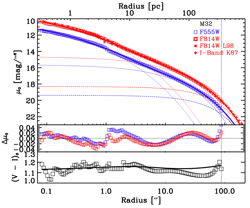
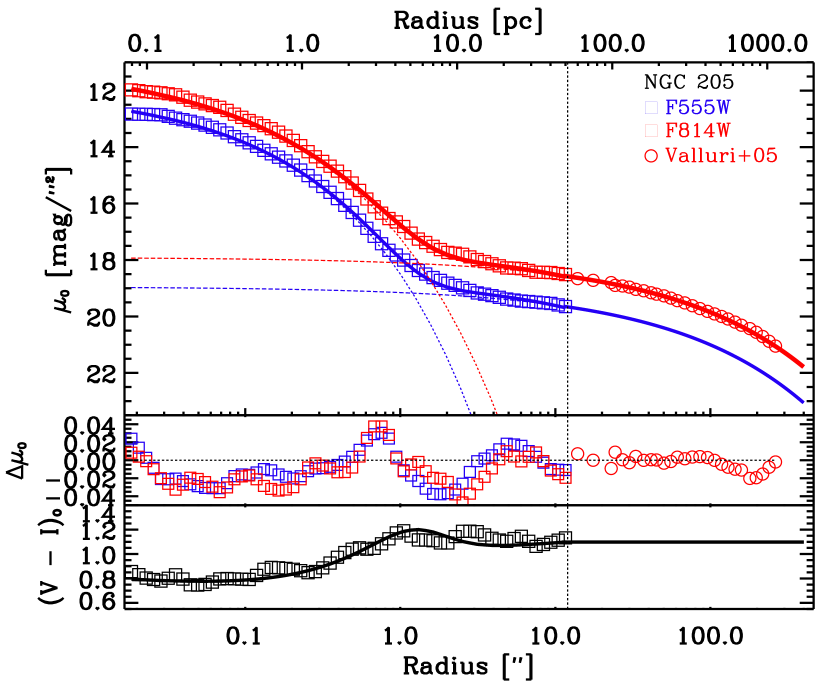
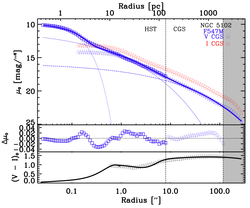
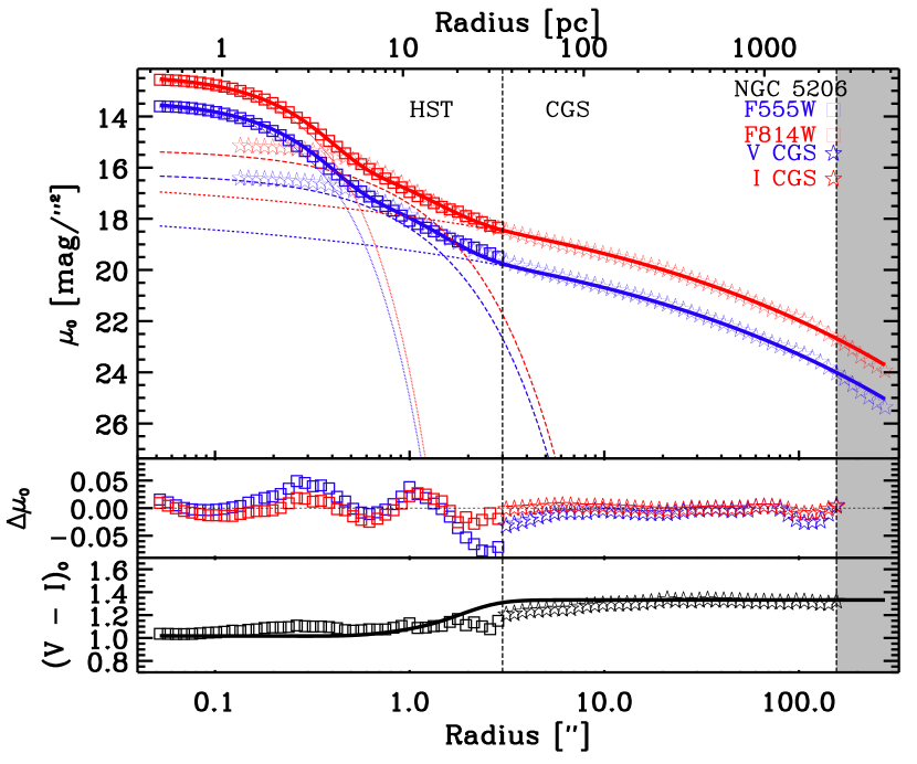
Figure 1.— The surface brightness profiles of each galaxy studied here. The profiles are constructed from a combination of ground-based and HST imaging. The blue lines show $V$/F555W/F547M profiles, while the red lines show $I$/F814W profiles. All magnitudes/colors are corrected for foreground extinction. Symbols show the data, while the best fitting 1D surface brightness profiles are shown as solid lines. Each component of the best-fit models are also plotted for visualization (the innermost Sérsic component is shown in dotted line, the second largest is shown as a dashed, and when present, the outermost component is shown in the long-dashed line). The residuals of the fits are shown in the middle-panel plots and the $(V-I)_{o}$ color profiles are illustrated in the bottom-panel plots including the data (open-black symbols) and the best-fit model (black solid line). Different symbols are plotted correspondingly to their data set, which are shown in the legend of each top panel. The inner and outer vertical dashed lines show the ends of the HST and ground-based data, respectively. The grey regions in the plots of NGC 5102 and NGC 5206 indicate the areas beyond our fitting radius.

4. Surface Brightness Profiles

4.1. Large Scale Structure from the one-dimensional (1D) surface brightness (SB) Profiles

To characterize the NSCs and create mass models for our targets, we first investigate the central SB profiles using HST imaging combined with larger scale SB profiles from the ground-based data. After fitting for the large scale properties of the galaxy, we fit the smaller scale structure near the center in Section 4.2 using GALFIT.

For our 1D profiles, we use the IRAF ellipse (Jedrzejewski, 1987) routine to extract fluxes in the annuli as a function of the major semi-axis. While extracting the fluxes, we allow the position angle (PA) and ellipticity ($\epsilon$) to vary.

Due to the small field of view (FOV) of the HST data, the sky background is not easy to estimate. To solve this problem, we use the existing ground-based data to estimate the sky backgrounds; the existing ground-based data include Kent (1987) and Lauer et al. (1998) for M32, Kent (1987) and Valluri et al. (2005) for NGC 205; and Carnegie-Irvine Galaxy Survey (CGS; Ho et al., 2011; Li et al., 2011; Huang et al., 2013) for NGC 5102 and NGC 5206. We use data at intermediate radii to match the HST SB and ground-based SB with shifts of $<$0.15 mags. Next we determine the sky background in the HST images by matching them out to larger radii. In the end, our 1D SB profiles are calibrated in Vega magnitudes (Sirianni et al., 2005) and are corrected for Galactic extinction (Table 1).

We fit the combined 1D SB profiles of each galaxy with multiple Sérsic profiles using the nonlinear least-squares IDL MPFIT function (Markwardt, 2009). Because we do not do PSF convolution, we use these fits to constrain just the outer components of the fit, the best fits are shown in Figure 1 and Table 5. The NGC 205 SB profiles are well fit by a double Sérsic function (NSC $+$ galaxy), however, the 1D SB of M32 requires two outer Sérsics profiles (the outermost Sérsic is an exponential) + NSC, while NGC 5102 and NGC 5206 require two NSC Sérsic components + a galaxy component based on their 2D fits. We note that our exponential disk component of M32 and the outer Sérsis component of NGC 205 are fully consistent with Graham (2002) and Graham & Spitler (2009), and these components will be fixed in 2D GALFIT (Section 4.2). The robustness of our 1D fits are tested by changing the outer boundaries in the ranges of 70$\arcsec$–90$\arcsec$, 100$\arcsec$–200$\arcsec$, 90$\arcsec$–110$\arcsec$, and 90$\arcsec$–120$\arcsec$ for M32, NGC 205, NGC 5102, and NGC 5206, respectively. The standard deviation of the Sérsic parameters from these fits was used to determine the errors; these errors are $<$10% in all cases. The fits are performed in multiple bands, enabling us to model the color variation.

We show the 1D SB profile fits, residuals, and $(V-I)_{\rm o}$ color of each galaxy in the top- middle-, and bottom-panel of each plot in Figure 1. These models agree well within the data with MEAN(ABS((data-model)/data) <5% for all four galaxies. M32 shows no radial color gradient, consistent with previous observations (Lauer et al., 1998). The other three galaxies show bluer colors toward their centers. We also note that we use these models only to constrain the outer Sérsic components of the galaxies, the best-fit inner components are derived from 2D modeling of the HST images.

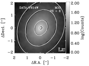
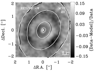
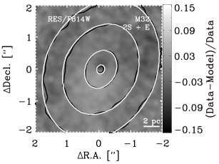
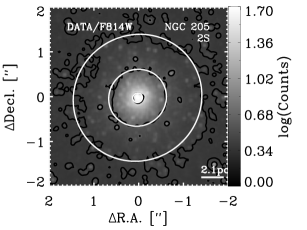
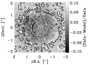
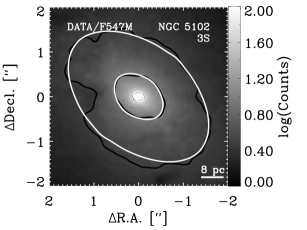
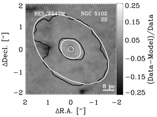
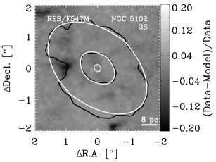
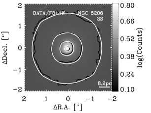
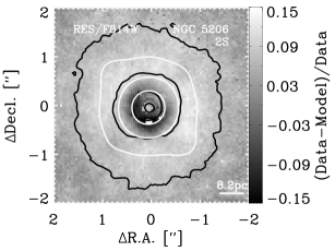
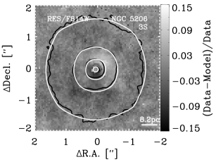
Figure 2.— Comparison of HST images to their GALFIT models for each galaxy. Left panels: the 2D HST/WFPC2 PC (M32, NGC 5102, NGC 5206) or ACS/HRC (NGC 205) images. Middle panels: the fractional residual (Data-Model)/Data between the HST imaging and their corresponding two-component GALFIT models. Right panels: fractional residuals from the three-components GALFIT models. The data and model contours are shown at the same levels of flux and radius in black and white repeating from the left to the right panels, respectively. All figures show East to the left, and North up.

Table 5GALFIT Models, Stellar Population Masses, and Luminosities of Galaxies in the Sample

Object

Filter

SB

$n_{i}$

$r_{\rm eff.,}$i

$r_{\rm eff.,}$i

$m_{i}$

PAi

b/ai

$\chi_{\rm r}^{2}$

$L_{\star}$,i

$M_{\star}$${}_{,i,\;\rm pop.}$

Comp.

($\arcsec$)

(pc)

(mag)

(∘)

($\times 10^{7}$$L_{\odot}$)

($\times 10^{7}$$M_{\odot}$)

(1)

(2)

(3)

(4)

(5)

(6)

(7)

(8)

(9)

(10)

(11)

(12)

(13)

Free PA

M32

F814W

2D

2.7$\pm$0.3

1.1$\pm$0.1

4.4$\pm$0.4

11.0$\pm$0.1

$-$23.4$\pm$0.5

0.75$\pm$0.03

1.10$\pm$0.10

1.45$\pm$0.24

NSC

2D

1.6$\pm$0.1

27.0$\pm$1.0

108$\pm$4

7.0$\pm$0.1

$-$24.7$\pm$0.4

0.79$\pm$0.07

1.7

43.5$\pm$4.0

79.4$\pm$10.3

Bulge

1D⋆

1

129

516

8.6

$-$25.0$\pm$0.7

0.79$\pm$0.05

9.96

19.3$\pm$2.5

Disk

Fixed PA

M32

F814W

2D

2.7$\pm$0.3

1.1$\pm$0.1

4.4$\pm$0.4

11.1$\pm$0.1

$-$25.0

0.75$\pm$0.09

1.10$\pm$0.10

1.45$\pm$0.25

NSC

2D

1.6$\pm$0.1

27.0$\pm$1.0

108$\pm$4

7.1$\pm$0.1

$-$25.0

0.79$\pm$0.11

2.0

43.8$\pm$4.1

78.0$\pm$10.4

Bulge

1D⋆

1

129

516

8.6

$-$25.0

0.79$\pm$0.08

10.00

19.3$\pm$2.5

Disk

Free PA

NGC 205

F814W

2D

1.6$\pm$0.2

0.3$\pm$0.1

1.3$\pm$0.4

13.6$\pm$0.4

$-$37.1$\pm$1.4

0.95$\pm$0.03

0.10$\pm$0.04

0.18$\pm$0.08

NSC

1D⋆

1.4

120

516

6.8

$-$40.4$\pm$1.0

0.90$\pm$0.07

5.5

55.7

97.2$\pm$15.2

Bulge

Fixed PA

NGC 205

F814W

2D

1.6$\pm$0.2

0.3$\pm$0.1

1.3$\pm$0.4

13.6$\pm$0.4

$-$40.4

0.95$\pm$0.06

0.10$\pm$0.04

0.18$\pm$0.08

NSC

1D⋆

1.4

120

516

6.8

$-$40.4

0.91$\pm$0.05

5.9

55.7

97.2$\pm$15.2

Bulge

Free PA

NGC 5102

F547M

2D

0.8$\pm$0.2

0.1$\pm$0.1

1.6$\pm$1.6

14.20$\pm$0.30

55.1$\pm$1.5

0.68$\pm$0.06

1.81$\pm$0.51

0.71$\pm$0.22

NSC1

2D

3.1$\pm$0.1

2.0$\pm$0.3

32.0$\pm$4.8

12.27$\pm$0.21

51.1$\pm$1.7

0.59$\pm$0.04

3.3

10.7$\pm$1.98

5.8$\pm$0.6

NSC2

1D⋆

3

75

1200

9.05

50.0

0.60$\pm$0.07

210

592$\pm$83

Bulge

Fixed PA

NGC 5102

F547M

2D

0.8$\pm$0.2

0.1$\pm$0.1

1.6$\pm$1.6

14.20$\pm$0.30

50.5

0.68$\pm$0.05

1.81$\pm$0.51

0.71$\pm$0.22

NSC1

2D

3.1$\pm$0.1

2.0$\pm$0.3

32.0$\pm$4.8

12.27$\pm$0.22

50.5

0.60$\pm$0.08

3.6

10.7$\pm$1.98

5.8$\pm$0.6

NSC2

1D⋆

3

75

1200

9.05

50.5

0.63$\pm$0.10

210

592$\pm$83

Bulge

Free PA

NGC 5206

F814W

2D

0.8$\pm$0.1

0.2$\pm$0.1

3.4$\pm$1.7

16.9$\pm$0.5

36.0$\pm$0.1

0.96$\pm$0.03

0.094$\pm$0.045

0.17$\pm$0.10

NSC1

2D

2.3$\pm$0.3

0.6$\pm$0.1

10.5$\pm$1.7

14.8$\pm$0.2

38.5$\pm$1.4

0.96$\pm$0.02

2.4

0.65$\pm$0.12

1.28$\pm$0.6

NSC2

1D⋆

2.57

58

986

10.1

38.6

0.98$\pm$0.01

123.3

241$\pm$47

Bulge

Fixed PA

NGC 5206

F814W

2D

0.8$\pm$0.1

0.2$\pm$0.1

3.4$\pm$1.7

16.9$\pm$0.5

38.3

0.96$\pm$0.03

0.094$\pm$0.045

0.17$\pm$0.10

NSC1

2D

2.3$\pm$0.3

0.6$\pm$0.1

10.2$\pm$1.7

14.8$\pm$0.2

38.3

0.97$\pm$0.03

2.7

0.65$\pm$0.12

1.28$\pm$0.27

NSC2

1D⋆

2.57

58

986

9.1

38.3

0.98$\pm$0.01

122.3

241$\pm$47

Bulge

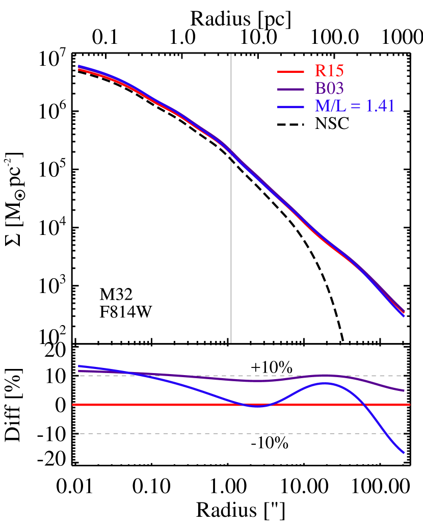
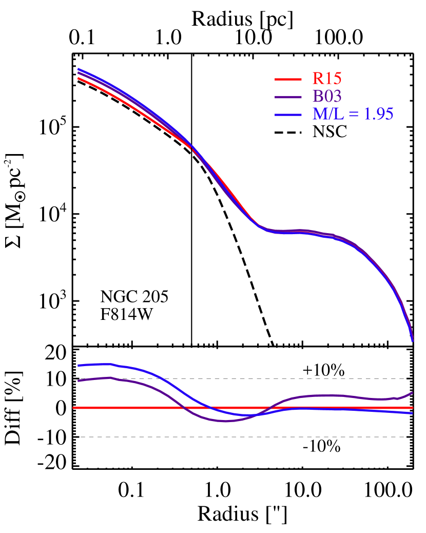
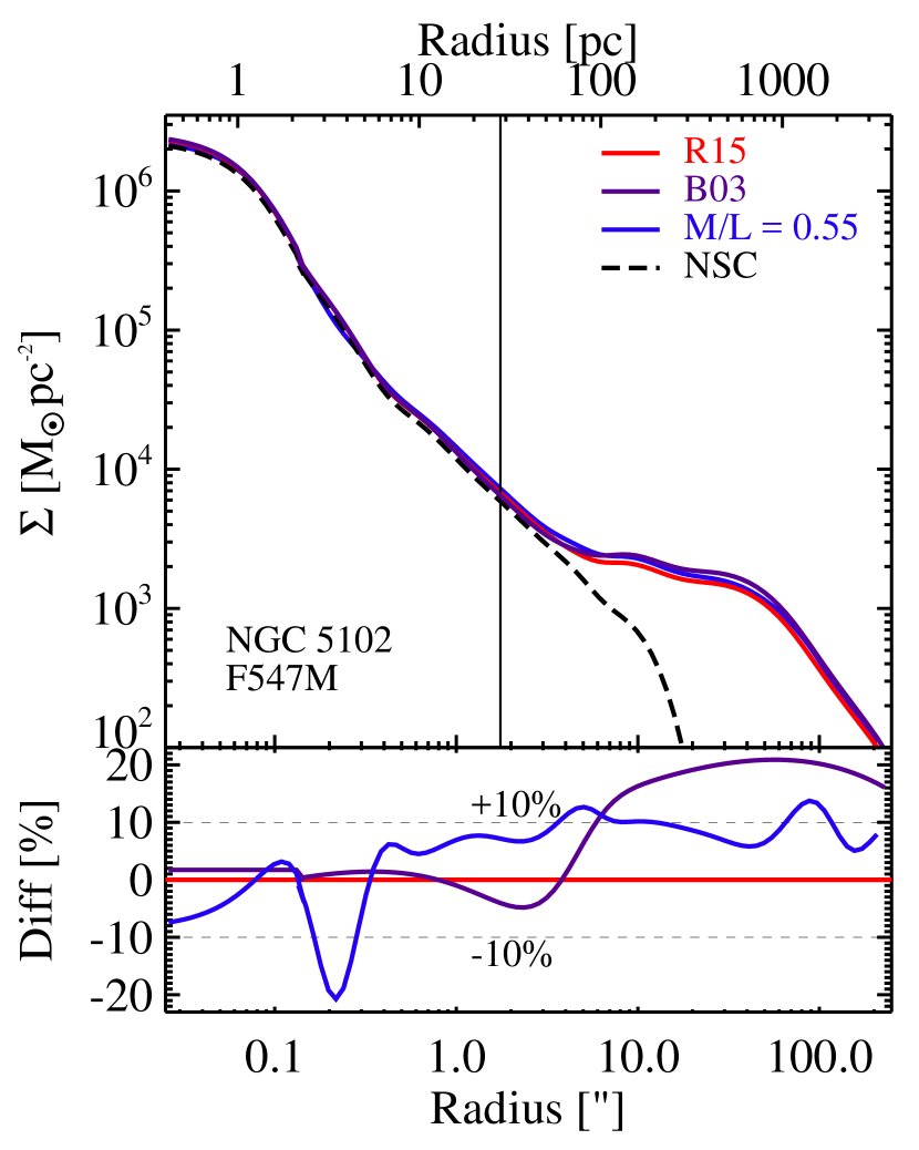
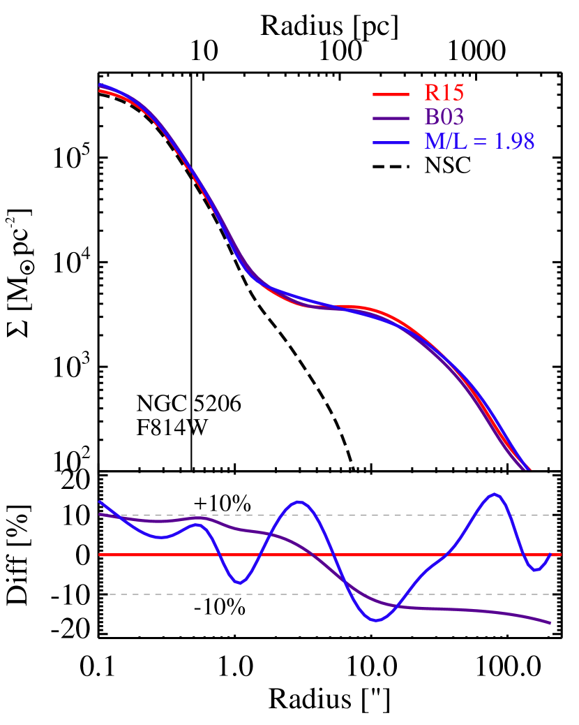
Figure 3.— Top panels: Comparison of the mass surface density models in each galaxy. These models are created using MGEs constructed from our GALFIT models. These MGEs are then multiplied by a M/L to get a mass surface density. For the constant M/L model (dark blue) the chosen M/L is discussed in Section 4.3. For the other mass models, an M/L is assigned to each MGE based on the color of the galaxy at the radius of the MGE using the R15 or B03 color–M/L relation (red/purple lines); we use the R15 model as our default. Dashed black lines show the NSCs in the R15 model; their effective radii are shown by vertical lines. Bottom panels: To compare the relative mass distribution of the three different mass profiles for each galaxy, we plot their fractional difference relative to the R15 color–M/L relation.

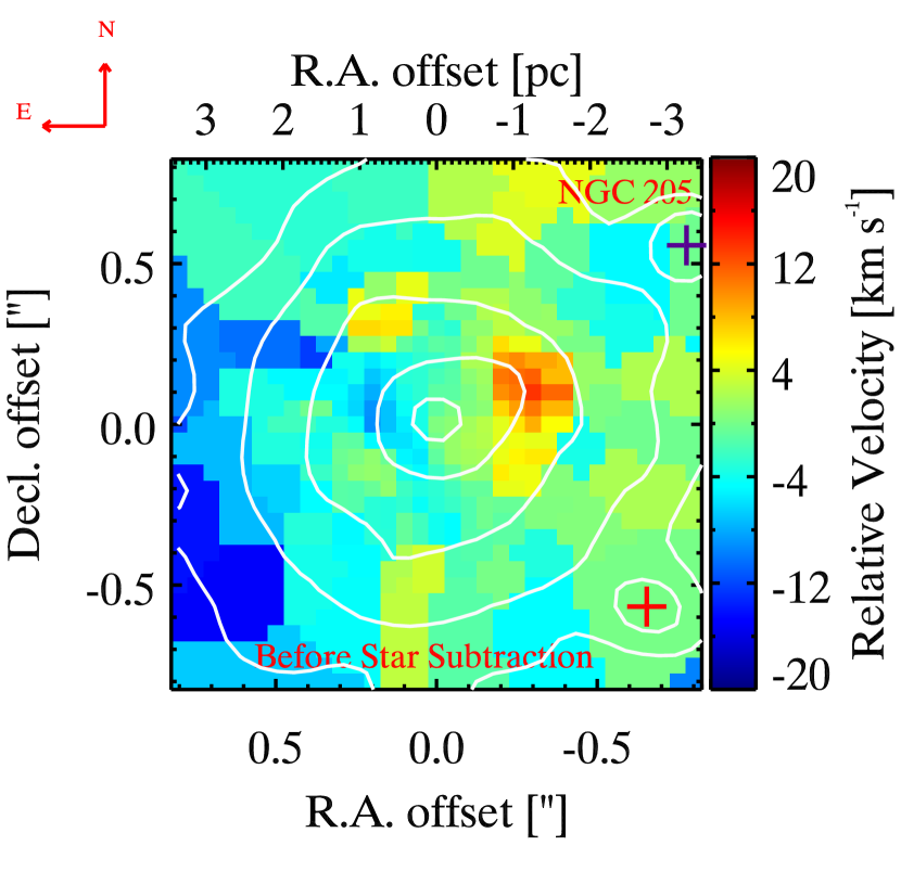
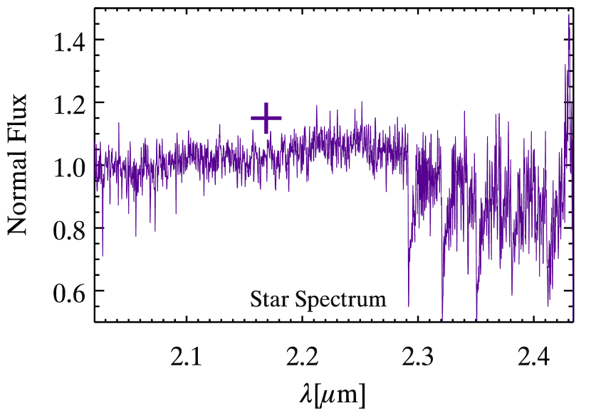
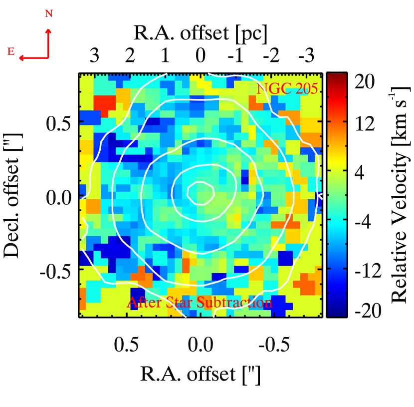
Figure 4.— Left panel: The radial velocity map derived from CO bandhead spectroscopy from Gemini/NIFS of NGC 205 before central resolved stars subtraction. The white intensity contours are plotted overlay on top of the map show those resolved star in the FOV with the two brights on north-west (purple plus) and south-west (red plus) of the map. Middle panel: The spectrum of the brightest purple plus star is shown in the same color respectively. Right panel: The radial velocity map derived from CO bandhead spectroscopy from Gemini/NIFS of NGC 205 after central resolved star subtraction (Section 5.2). The white intensity contours after the subtraction of resolved stars are now smoother.

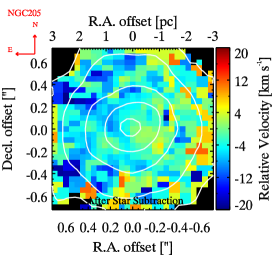
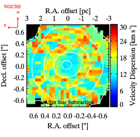
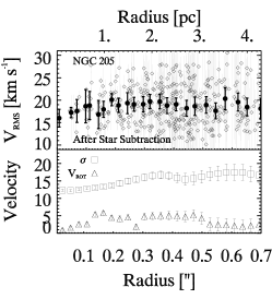
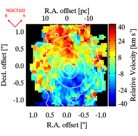
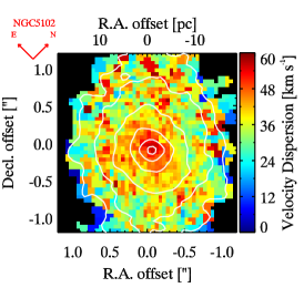
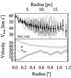
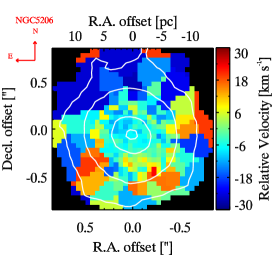
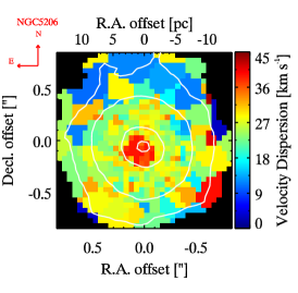
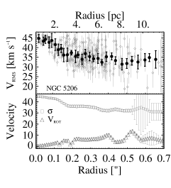
Figure 5.— Stellar kinematic maps derived from CO bandhead spectroscopy from Gemini/NIFS (NGC 205) and VLT/SINFONI (NGC 5102 and NGC 5206) spectroscopic data. Radial velocity maps are shown in the left column, and dispersion maps in the middle column. The radial velocity is shown relative to the systemic velocity of $-241\pm 2$ km s^-1(NGC 205), $472\pm 2$ km s^-1(NGC 5102), $573\pm 5$ km s^-1(NGC 5206). The top plots show the NGC 205 stellar kinematics after removing individual bright stars (Section 5.2). White contours show the stellar continuum; and the red arrows indicate the orientation. Kinematics are only plotted out to the radii where they are reliable; black pixels indicate data not used in the JAM modeling. In the right plots, the top-panel shows the $V_{\rm RMS}=\sqrt{V^{2}+\sigma^{2}}$ (open diamonds), with the filled black dots showing the bi-weighted $V_{\rm RMS}$ in the circular annuli. The error bars are $1\sigma$ deviations of the kinematic measurements of the Voronoi bins in the same annuli. The KINEMETRY decomposition (Krajnović et al., 2006) of dispersion (open squares) and rotation (open triangles) curves are shown in the bottom-panel.

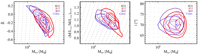
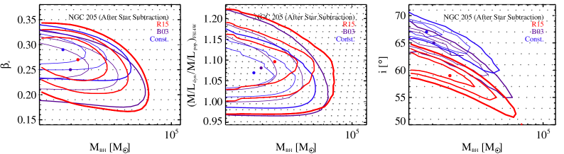
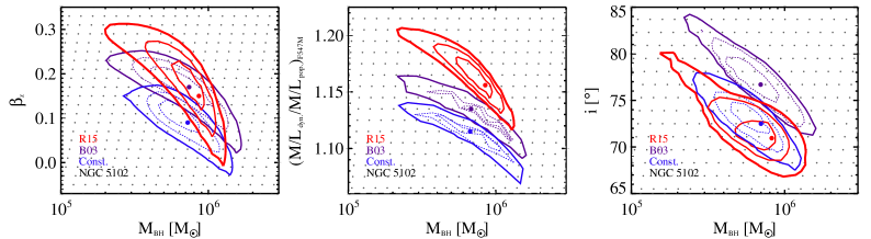
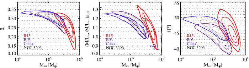
Figure 6.— Best-fit JAM models. The red contours and dot show our reference model in each galaxy based on the R15 color–M/L relation. The blue and purple contours and dots give the B03 and constant M/L mass models. Contours show $\Delta\chi^{2}$ = 2.30, 6.18 (dashed lines), and 11.83 (solid line) corresponding to 1$\sigma$, 2$\sigma$, and 3$\sigma$ confidence levels for two parameters after marginalizing over the other two parameters. The gray dots show the grid of models. The columns show the BH mass vs. the anisotropy, $\beta_{z}$ (left), the mass scaling factor, $\gamma=M/L_{\rm dyn.}/M/L_{\rm pop.}$ (center), and inclination, $i$ (right).

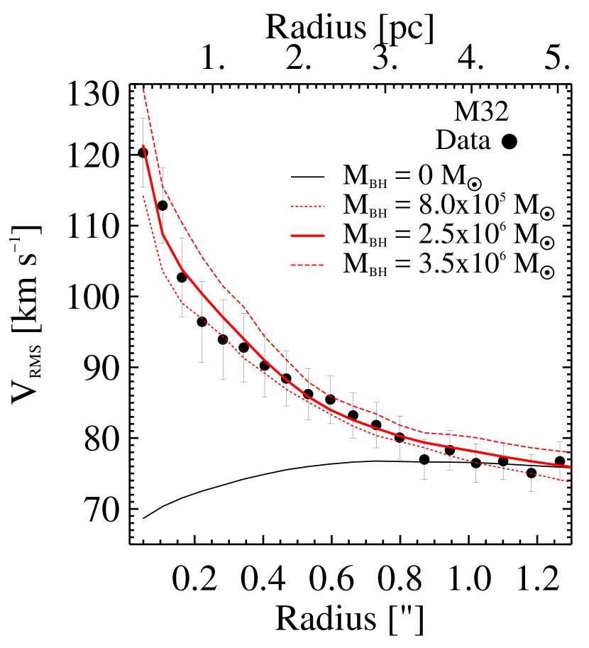
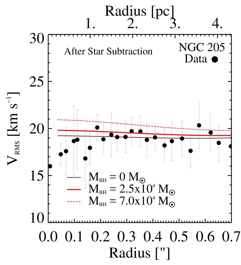
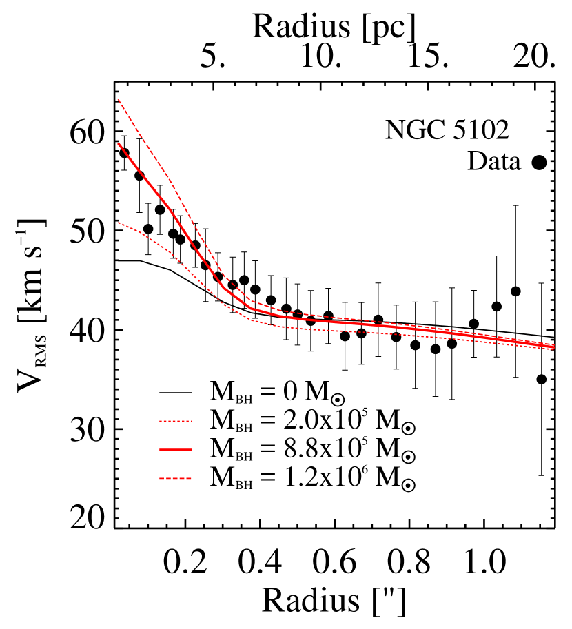
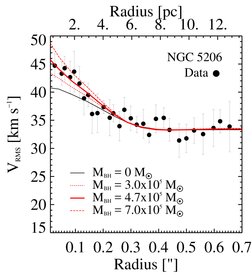
Figure 7.— 1D $V_{\rm RMS}$ vs. JAM predictions of mass models with varying BH masses. The red solid lines show our best-fit JAM models. Long-dashed and short-dashed lines indicate the upper and lower range of BH masses within 3$\sigma$ (see Figure 6 and Table 6), while the black line shows the best-fit JAM models without a BH. All models are fixed to the corresponding best-fit inclination angles of galaxies (column 9, Table 6) but varying for anisotropy, mass scaling ratio, and BH mass, which will be written in the form of ($\beta_{z}$, $\gamma$, $M_{\rm BH}$, $i$). The specific zero-mass and best-fit BH models plotted have (0.10, 1.20, 0$M_{\odot}$, 70^∘) and ($-$0.2, 1.08, $2.5\times 10^{6}$$M_{\odot}$, 70^∘) for M32, (0.27, 1.12, 0$M_{\odot}$, 63^∘) and (0.27, 1.10, $7.0\times 10^{4}$$M_{\odot}$, 55^∘) for NGC 205, (0.26, 1.19, 0$M_{\odot}$, 71.5^∘) and (0.15, 1.15, $8.8\times 10^{5}$$M_{\odot}$, 71.5^∘) for NGC 5102, and (0.30, 1.16, 0$M_{\odot}$, 44.5^∘) and (0.25, 1.06, $4.7\times 10^{5}$$M_{\odot}$, 45.5^∘) for NGC 5206. Both $V_{\rm RMS}$ profiles of spectroscopic data and their corresponding JAM models predictions are binned radially in the same manner for all galaxies as presented in the right panels of Figure 5. The error bars are $1\sigma$ deviations of the kinematic measurements of the Voronoi bins in the same annuli.

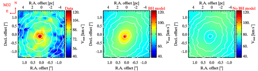
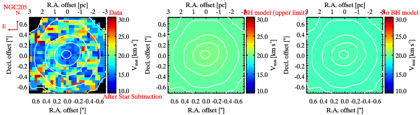
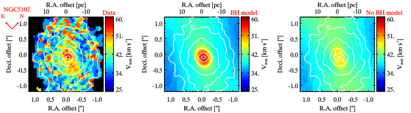
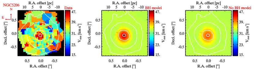
Figure 8.— A 2D data-model comparison of JAM models with and without BHs. The left panels show maps of $V_{\rm RMS}$ data in each galaxy, the middle panels show the best-fit JAM model 2D maps, and the right panels best-fit models without a BH. These models are the same as shown in 1D in Figure 7. The white contours show the continuum and red arrows the orientation.

4.2. NSC morphology from 2D GALFIT Models

Our dynamical models rely on the accurate measurements of the 2D stellar mass distribution near the centers of each galaxy. Moreover, the 2D SB profile is also important for quantifying the morphology of the NSCs. We model the HST images around the nucleus using GALFIT. GALFIT enables fitting with convolved models (using a PSF from Tiny Tim, Section 2.3), and excluding pixels using a bad pixel mask. The bad pixel mask is obtained using an initial GALFIT run without a mask; we mask all pixels with absolute pixel values >$3\sigma$ than the median value in the residual images (Data-Model). Based on our 1D SB profile, we chose to fit NGC 205 with a double-Sérsic function (2S), M32 is fitted with a 2S + Exponential disk (2S + E). For NGC 5102 and NGC 5206 we find the nuclear regions require two components (Figure 2), and thus these are fitted with triple-Sérsic functions (3S). The initial guesses were input with the best-fit parameters from the 1D SB fits with fixed parameters for the outermost Sérsic or E component except for the PA and axis ratio ($b/a$). For the purpose of creating mass models for dynamical modeling of BH masses measurements, we repeat these 2D fit with fixed PA in all Sérsic components because the Jeans Anisotropic Models (JAM; Cappellari, 2008) assume axisymmetry, which implies a constant PA.

The left column of Figure 2 show the F814W images of M32, NGC 205, and NGC 5206 and F547M image of NGC 5102, while the middle column show their relative errors between the HST images and their 2S models, (Data-Model)/Data. The right column also show these relative errors between the HST images and their 2S + E (M32) or 3S (NGC 5102 and NGC 5206) models. The contours on each panel show both data (black) and model (white) at the same radius and flux level to highlight the regions of agreement and disagreement between data and models. Excluding masked regions (and point sources in NGC 205), the maximum errors on the individual fits are <9%, 15%, 13%, and 10% for M32, NGC 205, NGC 5102, and NGC 5206, respectively. The parameters of the best-fit GALFIT models are shown in Columns 4–9 of Table 5; errors are scaled based on the 1D errors in the components estimated in Section 4.1 due to their dominant over the GALFIT errors. We note that the 2D GALFIT models give Sérsic parameters consistent to that of 1D SB profiles fit, especially for the middle Sérsic components where the PSF effects are minimal. We note that our NSC component in M32 is significantly less luminous than the 1D SB profile given in Graham & Spitler (2009); we believe this is at least in part due to their normalization in the SB profile, which is nearly a magnitude higher than that derived here.

Next, we use the final fixed-PA 2D GALFIT Sérsic models to create multi-Gaussian expansion (MGEs; Emsellem et al., 1994a, b; Cappellari & Emsellem, 2004) models. These MGEs are comprised of a total of 18, 10, 14, and 14 Gaussians to provide a satisfactory fit to the surface mass density profiles of M32, NGC 205, NGC 5102, and NGC 5206 respectively. We fit our MGEs out to $\sim$$110\farcs 0$ for M32 and NGC 5206, $15\farcs 0$ for NGC 205, $21\farcs 0$ for NGC 5102 and obtain the mass models by straightforward multiplying the M/L profiles with the 2D light GALFIT MGEs at the corresponding radii. We choose to parameterize the mass models using GALFIT (as opposed to using the fit_sectors_mge code) because (1) it enables us to properly incorporate the complex HST PSF, and (2) it enables simple separation of NSC and galaxy components.

4.3. Color–M/L Relations

To turn our stellar luminosity profiles into stellar mass profiles, we assume a M/L–color relation. There is a strong correlation between the color and the M/L of a stellar population: we use two different color–M/L relations including the Bell et al. (2003) (hereafter B03), Roediger & Courteau (2015) (henceforth R15) color–M/L correlations, as well as models with constant M/L. This is similar to the method presented by Nguyen et al. (2017) for analysis of the NGC 404 nucleus. For our best-fit models we use the R15 relation, which was found by Nguyen et al. (2017) to be within 1$\sigma$ of the color–M/L relation derived from stellar population fits to STIS data within the nucleus. The B03 and constant M/L models are used to assess the systematic uncertainties in our mass models. The B03 and R15 relations are built based on the $(V-I)_{0}$ color profiles in the bottom panel of each plot in Figure 1, except in NGC 5102. For NGC 5102, we use the $(B-V)_{0}$ color estimated from the combined HST F547M–F656N data at small radii and F450W–F569W data at larger radii as described in the appendix A.

We also create mass models with a constant central M/L. For these models, we take a reasonable reference value for the M/L, but still allow these values to be scaled in our dynamical models, just as for the varying M/L models. We note that these models are not used in any of our final results, but are used to analyze potential systematic errors in our dynamical modeling. The reference values used for the constant M/L models are:

• M32: We use $M/L_{I}=1.41$ ($M_{\odot}$/$L_{\odot}$) based on the Schwarzschild model fits to Sauron data from Cappellari et al. (2006).

• NGC 205: We use a similar nucleus of $M/L_{I}=1.95$ ($M_{\odot}$/$L_{\odot}$) to that based on Schwarzschild models fit to STIS kinematics by ($M/L_{I}=1.94$ ($M_{\odot}$/$L_{\odot}$), Valluri et al., 2005); note that this is the value found for the nucleus (they find a significantly higher M/L for the galaxy as a whole).

• NGC 5102: We use M/L${}_{V}=0.55$ ($M_{\odot}$/$L_{\odot}$) based on the stellar population model fits near the center of the galaxy from Figure 11 of Mitzkus et al. (2017) which assume use the MILES libraries with a Salpeter IMF.

• NGC 5206: We use the photometric $M/L_{I}=1.98$ ($M_{\odot}$/$L_{\odot}$) based on the color $(V-I)_{o}=1.1$ and using estimates from Bell et al. (2003); Bruzual & Charlot (2003).

4.4. Mass Models

We create our final mass models for use in our dynamical modeling by multiplying the MGE luminosity created from the 2D GALFIT fit models of the images with PSF-deconvolution (Section 4.2) with the M/L profiles discussed in Section 4.3. We fit the MGE luminosity by using the sectors_photometry + mge_fit_sectors IDL package. During these fits we set their PAs and axial ratios of the Gaussians to be constants as their values obtained in GALFIT. More specifically, in NGC 5102 we calculate the $V$–band M/L and apply this to the F547M data, while in the others, we calculate $I$–band M/Ls and apply these to the F814W data.

The top-panel in each plot of Figure 3 shows the mass surface density and the bottom-panel shows the relative error of the M/L profile relative to the R15 color–M/L correlation for each galaxy. It is clear that the R15 color–M/L correlation (red line) predicts less mass at the center of each galaxy than the prediction of B03 color–M/L correlation (purple line). However, the assumption of constant M/Ls (blue line) predict more mass at the centers but less mass at larger radii than the predictions of both B03 and R15 color–M/L correlation. This is as expected based on the bluer centers and consequently lower M/Ls at the centers. The MGEs of mass surface densities of M32, NGC 205, NGC 5102, and NGC 5206 are presented in column (2) of Table 11 (Appendix B).

4.5. $K$–Band Luminosities

Together with the stellar mass distribution, the dynamical models also require as input the distribution of the stellar tracer population from which the kinematics is obtained. Given that the kinematics was derived in the $K$–band, which covers the wavelengths from 2.29 to 2.34$\mu$m, we create high-resolution synthetic images in that band (Ahn et al., 2017). We do not use the $K$–band images obtained from the IFU observations directly as they have lower resolution and too limited FOV. To make these we employ Padova SSP model (Bressan et al., 2012) to fit color–color correlations. The purpose of this is to transform our HST imaging of F555W and F814W (of M32, NGC 205, and NGC 5206) into $K$–band images. Specifically, we fit the linear correlations of HST F555W–F814W vs. F814W–$K$ based on the specific nucleus stellar populations and metallicities for M32 ($Z=0.019$, Corbin et al., 2001), NGC 205 ($Z=0.008$, Butler & Martínez-Delgado, 2005), and NGC 5206 ($Z=0.004-0.008$; N. Kacharov et al., in prep.). We use these to create $K$–band images based on the reference HST images (i.e., we add the color correction to the F814W image). These $K$ band images are similar to the $I$–band images, with deviations in the SB profile being comparable to differences between mass models shown in Figure 3.

In order to create a $K$–band image for NGC 5102, we use its F450W–F569W colors, which are inferred from the F547M–F656N data as described in the appendix A. Next, we fit a linear correlation of HST F450W–F569W vs. F569W–$K$ using metallicities $Z=0.004$ (Davidge, 2015), then infer for its $K$–band images. We then fit the MGEs using the mge_fit_sectors IDL package. The MGEs $K$–band luminosity surface densities of M32, NGC 205, NGC 5102, and NGC 5206 are given in column (1) Table 11 (Appendix B).

5. Stellar Kinematics Results

We use adaptive optics NIFS and SINFONI spectroscopy to determine the nuclear stellar kinematics in all four galaxies. We first re-bin spatial pixels within each wavelength of the data cube using the Voronoi binning method (Cappellari & Copin, 2003) to obtain S/N $\gtrsim$ 25 per spectral pixel. Next, we use the pPXF method (Cappellari & Emsellem, 2004; Cappellari, 2017) to derive the stellar kinematics from the CO band-heads of the NIFS and SINFONI spectroscopy in the wavelength range of 2.280–2.395 $\mu$m and determine the line-of-sight velocity distribution (LOSVD). We fit only a Gaussian LOSVD, measuring the radial velocity ($V$) and dispersion ($\sigma$) using high spectral resolution of stellar templates of eight supergiant, giant, and main-sequence stars with spectral types between G and M with all luminosity classes (Wallace & Hinkle, 1996). These templates are matched to the resolution of the observations by convolving them by a Gaussian with dispersion equal to that of the line-spread function (LSF) of the observed spectra at every wavelength. These LSFs are determined from sky lines. For NIFS, the LSF is quite Gaussian with a FWHM $\sim$4.2 Å, but the width varies across the FOV (e.g., Seth, 2010). However, the SINFONI LSF appears to be significantly non-Gaussian as seen from the shape of the OH sky lines. To characterize the shape of the LSF and its potential variation across the FOV, we reduced the sky frames in the same way as the science frames, with the difference that we did not subtract the sky. We then combined the reduced sky cubes using the same dither pattern as the science frames. This ensured that the measured LSF on the resulting sky lines fully resembles the one on the object lines. From these dithered sky lines we measured the LSF. We used 6 isolated, strong sky lines, all having close doublets, except one (the 21,995 Å line), to measure the spectral resolution across the detector. Since the LSF appears to be constant along rows (constant y values), the sky cubes were collapsed along the y-direction.

Sky emissions OH-lines can be described as a delta function, $\delta_{\lambda}$. Once they reach the spectrograph they will be dispersed so that the intensity pattern is redistributed with wavelength according to the LSF of the instrument. Since we know the central wavelength of the sky emission lines we assume that their shapes represent the LSF. Once located, the peak values in the spectra and a region around the peaks is defined, the continuum is subtracted, the line flux is normalized to the peak flux and finally the lines are summed up.

The spectral resolution across the detector has a median value of 6.32 Å FWHM ($\frac{\lambda}{\Delta\lambda}=3820$) with values ranging from 5.46 to 6.7 Å FWHM (R $\sim$ 3440 – 4300). The last step before the kinematic extraction is to perform the same binning on the LSF cube as for the science cube. This varying LSF is then used in the kinematic extraction with pPXF.

To obtain optimal kinematics from the SINFONI data we had to correct for several effects: (1) a scattered light component and (2) velocity differences between individual cubes. For the first issue, the SINFONI data cubes have imperfect sky subtraction, with clear additive residuals remaining despite subtraction of sky cubes. These residuals appear to have a uniform spectrum that is spatially constant across the field, however the residuals are not clearly identified as sky or stellar spectra. To remove these residuals, we create a median residual spectrum for each individual data cube using pixels beyond $1\farcs 3$ radius and subtract it from all spaxels in the cube. This subtraction greatly improved the quality of our kinematic fits to our final combined data cube, but we note that this is likely also subtracting some galaxy light from each pixel. Second, fits to sky lines revealed variations in the wavelength solutions corresponding to velocity offsets of up to 20 km s^-1 between individual data cubes. Therefore before combining the cubes, we applied a velocity shift to correct these shifts; 4/12 cubes for NGC 5102 and 3/12 cubes for NGC 5206 were shifted before combining bringing the radial velocity errors $\lesssim$2 km s^-1 among the cubes to their means for both galaxies. We note however that applying these velocity shifts had minimal impact ($<$0.5 km s^-1) on the derived dispersions. The systemic velocity in each galaxy was estimated by taking a median of pixels with radii $<$$0\farcs 15$, and is listed in Table 4.

To calculate the errors on the LOSVD, we add Gaussian random errors to each spectral pixel and apply Monte Carlo simulations to re-run the pPXF code. The errors used differ in NIFS and SINFONI; for NIFS we have an error spectrum available, and these are used to run the Monte Carlo, while with SINFONI, no error spectrum is available, and we therefore use the standard deviation of the pPXF fit residuals as a uniform error on each pixel. We test further the robustness of our kinematic results by (1) fitting the spectra toward the short wavelength range 2.280–2.338 $\mu$m of the CO band-heads (the highest S/N portion of the CO bandhead) and (2) using the PHOENIX model spectra (Husser et al., 2013), which have higher resolution ($R=500,000$ or 0.6 km s^-1) than the Wallace & Hinkle (1996) ($R=45,000$ or 6.67 km s^-1) templates. We find consistent kinematic results within the errors with (1) returning dispersions  1–2 km s^-1 higher than the full spectral range, while (2) yields fully consistent results. We also verified our SINFONI kinematic errors by combining independent subsets of the data and identical binning and found that their distribution had a scatter similar to the error; a similar verification of the NIFS errors was done in Seth et al. (2014). This analysis indicates that the radial velocities and dispersion errors range from 0.5–20 km s^-1. These kinematic data are presented in Table 8, 9, and 10 for NGC 205, NGC 5102, and NGC 5206 respectively in the appendix B, except for M32, which was published in Table 1 of Seth (2010).

Due to increased systematic errors affecting our kinematic measurements at low surface brightness (where many pixels are binned together), we eliminate the outermost bins beyond an ellipse with semi-major axes of 1$\farcs$3, 1$\farcs$2, 0$\farcs$7, and 0$\farcs$7 in M32, NGC 5102, NGC 5206, and NGC 205. In general, we find that in the noisy data in outer regions we overestimate our $V_{\rm RMS}$ values. For instance in the M32 data published in Seth (2010), we find a rise in $V_{\rm RMS}$ beyond 1$\farcs$3, however comparison with data from Verolme et al. (2002) suggests this rise may be due to systematic error, and is not used in the remainder of our analysis. In addition, we only plot and fit bins with dispersion and velocity errors $<$15 km s^-1. We correct the systemic velocities (then radial velocities) for the barycentric correction (37 km s^-1, 20 km s^-1, $-$20 km s^-1, and $-$37 km s^-1 for M32, NGC 205, NGC 5102, and NGC 5206). The systemic velocities are determined from the central velocity as references and double checked with using the fit_kinematic_pa IDL package.

The final kinematic maps for NGC 205, NGC 5102 and NGC 5206 are shown in Figure 5. The left column shows the radial velocity maps, the middle column shows the velocity dispersion maps. The right most column shows the $V_{\rm RMS}$ measurements (open gray diamonds with error bars, top panel) and the bi-weighted in the circular annuli (fill black dots with error bars). The bottom panel of the right column shows the results of KINEMETRY fits (Krajnović et al., 2006), which determines the best-fit rotation and dispersion profiles along ellipses. We discuss the kinematics for each galaxy below.

5.1. M32

The kinematics of M32 were derived with pPXF using a four-order of Gauss–Hermite series including $V$, $\sigma$, skewness ($h_{3}$), and kurtosis ($h_{4}$) (Seth, 2010). These measurements are the highest quality kinematic data available that resolve the sphere-of-influence (SOI) of the BH. These kinematics show a very clear signature of a rotating and disky elliptical galaxy with strong rotation at a PA of $-25$^∘ (E of N) with an amplitude of $\sim$55 km s^-1 beyond the radius of $0\farcs 3$ with the maximum of $V/\sigma$ reaching 0.76 at $r=0\farcs 5$ (2 pc). The dispersion has a peak of $\sim$120 km s^-1, which we will show is due to the influence of the BH, and flattens out at $\sim$76 km s^-1 beyond $0\farcs 5$.

5.2. NGC 205

Of the nuclei considered here, NGC 205 is by far the one most dominated by individual stars. These are clearly visible in the HST images (Figure 2), and their effects can be seen in our kinematics maps. These maps show bright individual stars that often have decreased dispersion and larger offsets from the systemic velocity, and therefore we have attempted to remove them before deriving the kinematics as done in Kamann et al. (2013). The spectrum of the star weighted by the PSF was subtracted from all adjacent spectra of the cube. We summarize this process briefly here. First, we identify bright stars in the FOV of NIFS data manually by-eye and note down their approximate spaxel coordinates in all layers of the data cube; there are 32 of these identified bright stars in total. Second, we estimate PSFs for these stars that are well-described analytically either by Moffat or double-Gaussian; the differences between these two PSF representations are small, but we use the Moffat profile in our final analysis. Next, we perform a combined PSF fit for all identified stars; in this analysis, we model the contribution from the galaxy core as an additional component that is smoothly varying spatially. Third, we obtain spectra for all identified stars so that their information were used to subtract off from each layer of the cube. Finally, we use this star-subtracted cube to determine the kinematics of underlying background light of the galaxy.

We show our original map of relative velocity in the left panel of Figure 4. One of the subtracted stellar spectra is shown in the middle panel, while velocity map after the stellar subtraction is shown in the right panel. Subtraction of stars yields a much smoother velocity map and isophotal contours than our original map. The complete kinematic maps determined after star subtraction are shown in the top row plots of Figure 5. We use this map for all further analysis, but also include the original map in tests on the robustness of our results.

We examine the stellar rotational velocity ($V$) and dispersion velocity ($\sigma_{\star}$) of NGC 205. The dispersion velocity drops to $\sim$15 km s^-1 within the $0\farcs 2$ radius and reaches $\sim$23 km s^-1 in the outer annulus of $0\farcs 2$–$0\farcs 8$. This dispersion velocity map is consistent with the radial dispersion profile obtained from HST/STIS data of the NGC 205 nucleus (Valluri et al., 2005) at the radius >$0\farcs 2$, although we find a slightly lower dispersion at the very nucleus than Valluri et al. (2005) ($\Delta$$\sigma\sim 3$ km s^-1). This difference in dispersions is $\sim$1 km s^-1 higher the velocity dispersion errors of the central spectral bins (Table 8 in Appendix B). However, we caution that both sets of kinematics are close to the spectral resolution limits of the data. However, with the high S/N of the central bins, and using our careful LSF determination, we believe we can reliably recover dispersions even at $\sim$15 km s^-1(Cappellari, 2017).

The $V_{\rm RMS}=\sqrt{V^{2}+\sigma^{2}}$ profile has a value of $20\pm 5$ km s^-1 out to $0\farcs 7$. The maximum $V/\sigma\sim 0.33$ occurs at $0\farcs 6$ (2.6 pc), and this low level of rotation is seen throughout the cluster.

5.3. NGC 5102

The radial velocity map of the NGC 5102 nucleus shows clear rotation. This rotation reaches an amplitude of $\sim$30 km s^-1at $0\farcs 6$ from the nucleus. Beyond this radius, the rotation curve is flat out to the edge of our data. The dispersion is fairly flat at $\sim$42 km s^-1 from $r=0\farcs 3$–$1\farcs 2$ with a peak at the center reaching $59\pm 1$ km s^-1. The maximum $V/\sigma$ is $\sim$0.7 at $0\farcs 6$. This suggests the second Sérsic component, which is identified as part of the NSC, and is the most flattened component, may be strongly rotating. This components position in the $V/\sigma$ vs. $\epsilon$ ($\epsilon=0.4$ and $V/\sigma=0.7$) is consistent with a rotationally flattened system, especially given the best-fit inclination of $\sim$71^∘ we derive below.

Our kinematics are consistent with those from Mitzkus et al. (2017), who use MUSE spectroscopy to measure kinematics out to radii of $\sim$30$\arcsec$. On larger scales they find the galaxy has two counter-rotating stellar disks, with maximum rotation amplitudes of $\sim$20 km s^-1and dispersions very similar to our measured dispersion throughout the central $\sim$10$\arcsec$.

5.4. NGC 5206

The radial velocity map of NGC520 shows a small but significant rotation signal in the nucleus; this rotation appears to gradually rise outwards with a maximum amplitude of 10–15 km s^-1 at $0\farcs 5$. Our decomposition of the nucleus shows a nearly round system ($b/a=0.96$) for both NSC components, however, the maximum $V/\sigma_{\star}\sim 0.3$ at $0\farcs 5$ suggests the outer of these two components may be more strongly rotating. Similar to NGC 5102, the NGC 5206 dispersion map shows a fairly flat dispersion of 33 km s^-1 from $r=0\farcs 4$–$0\farcs 7$, increasing to 46 km s^-1at the center.

6. Stellar Dynamical Modeling and BH Mass Estimates

In this section, we fit the stellar kinematics using JAM models and present estimates of the BH masses.

Table 6Gemini/NIFS and VLT/SINFONI Jeans modeling best-fit results

Object	Filter	Color–M/L	$M_{\rm BH}$	$\beta_{\rm z}$	$\gamma$	$i$	No. of Bins	$\chi^{2}_{\rm r}$	$\chi^{2}_{\rm r,\;noBH}$	$r_{\rm g,\;dyn.}$	$r_{\rm g,\;dyn.}$
			($M_{\odot}$)			(∘)				($\arcsec$)	(pc)
(1)	(2)	(3)	(4)	(5)	(6)	(7)	(8)	(9)	(10)	(11)	(12)
M32	F814WG	R15	$2.5^{+0.6}_{-1.0}\times 10^{6}$	$-0.20^{+0.30}_{-0.35}$	$1.08^{+0.20}_{-0.30}$	$70.0^{+6.0}_{-6.0}$	1354	1.12	6.72	0.404	1.61
NGC 205	F814WG	R15	$2.5^{+4.7}_{-2.5}\times 10^{4}$	$0.27^{+0.07}_{-0.10}$	$1.10^{+0.10}_{-0.18}$	$59.0^{+5.0}_{-8.0}$	256	1.24	1.20	0.033	0.14
NGC 5102	F547MG	R15	$8.8^{+4.2}_{-6.6}\times 10^{5}$	$0.15^{+0.16}_{-0.16}$	$1.15^{+0.06}_{-0.03}$	$71.5^{+9.0}_{-4.0}$	1017	1.12	3.57	0.070	1.20
NGC 5206	F814WG	R15	$4.7^{+2.3}_{-3.4}\times 10^{5}$	$0.25^{+0.08}_{-0.12}$	$1.06^{+0.05}_{-0.05}$	$44.0^{+8.5}_{-5.0}$	240	1.20	2.69	0.058	1.00

6.1. Jeans Anisotropic Models

We create dynamical models using the Jeans anisotropic models (JAM) of Cappellari (2008). Given the strong gradients in the stellar population of some of the galaxies, the mass-follows-light assumption is not generally acceptable. For this reason we distinguish the parametrization of the stellar mass, from that of the tracer population. This approach was also used for the same reason in the JAM models by Ahn et al. (2017); Li et al. (2017); Mitzkus et al. (2017); Nguyen et al. (2017); Poci et al. (2017); Thater et al. (2017). Specifically, we used the MGEs derived using the default R15 color–relation to parametrize the stellar mass, but we adopted the $K$–band luminosity MGEs to parametrize the tracer population in JAM. We use JAM to predict the second velocity moment, $V_{\rm RMS}=\sqrt{V^{2}+\sigma^{2}}$ – where $V$ is the radial velocity relative to the systemic velocity and $\sigma$ is the line-of-sight velocity dispersion (Section 5). The JAM models have four free parameters: BH mass ($M_{\rm BH}$), mass scaling factor ($\gamma=(M/L_{\rm dyn.})/(M/L_{\rm pop.}$)) assuming Salpeter IMF, anisotropy ($\beta_{z}$), and inclination angle ($i$), which relate the gravitational potential to the second velocity moments of the stellar velocity distribution. These second velocity moment predictions are projected into the observational space to predict the $V_{\rm RMS}$ in each kinematic bin using the luminosity model (synthetic $K$–band luminosity) and kinematic PSF. The anisotropy parameter ($\beta_{z}$) relates the velocity dispersion in the radial direction ($\sigma_{R}$) and z-direction ($\sigma_{z}$): $\beta_{z}=1-\sigma_{z}^{2}/\sigma_{R}^{2}$ assuming the velocity ellipsoid is aligned with cylindrical coordinates. The predicted $V_{\rm RMS}$ is compared to the observations, and a $\chi^{2}$ is determined for each model. The number of kinematic bins for the four galaxies are shown in Column 8 of Table 6. To find the best-fit parameters, we construct a grid of values for the four parameters ($\beta_{z}$, $\gamma$, $M_{\rm BH}$, $i$). For each triplet parameters of ($\beta_{z}$, $M_{\rm BH}$, $i$), we linearly scale $\gamma$ parameter to match the data in a $\chi^{2}$ evaluation. We run coarse grids in our parameters to isolate the regions with acceptable models, and then run finer grids over those regions as shown in Figure 6.

Figure 6 shows $\chi^{2}$ contours as a function of $M_{\rm BH}$ vs. $\beta_{z}$ (left), $M_{\rm BH}$ vs. $\gamma$ (middle), and $M_{\rm BH}$ vs. $i$ (right). The best-fit BH masses are shown by red dots with three contours showing the 1$\sigma$, 2$\sigma$ (thin red lines), and 3$\sigma$ (thick red line) levels or $\Delta\chi^{2}$ = 2.30 ($\sim$68%), 6.18 ($\sim$97%), and 11.81 ($\sim$99.7%) after marginalizing over the other two parameters. The best-fit $M_{\rm BH}$, $\beta_{z}$, $\gamma$, and $i$, and minimum reduced $\chi^{2}$ are shown Table 6. We quote our uncertainties below on the BH mass and other parameters at the 3$\sigma$ level. Given the restrictions JAM models place on the orbital freedom of the system (relative to e.g., Schwarzschild models), it is common to use 3$\sigma$ limits/detections in quoting BH masses (see Seth et al. (2014) and Section 4.3.1 of Nguyen et al. (2017) for additional discussion).

6.1.1 M32

The best-fit JAM model of M32 gives $M_{\rm BH}$ $=2.5^{+0.6}_{-1.0}\times 10^{6}$$M_{\odot}$, $\beta_{z}=-0.20^{+0.30}_{-0.35}$, $\gamma=1.08^{+0.20}_{-0.30}$, and $i=70$^∘${}^{+6}_{-6}$. We note the wide range in uncertainty in $\beta_{z}$ is likely due to the bulk of our kinematic data lying within the SOI of the BH. Our BH mass, M/L and $i$ estimates are fully consistent with values presented in Verolme et al. (2002), Cappellari et al. (2006), and van den Bosch & de Zeeuw (2010) after correcting to common distance of 0.79 Mpc and correct for extinction $A_{B}=0.177$ mag (Schlafly & Finkbeiner, 2011) and assuming A_I = A_B/2.22. The consistency of the BH masses in M32 shows the good agreement between JAM and Schwarzschild modeling techniques (see Section 6.2.3).

6.1.2 NGC 205

The JAM models of NGC 205 are compared to the kinematics derived after subtracting off bright stars in the nucleus (see Section 5.2). The data is consistent with no BH even at the 1$\sigma$ level, and we find a 3$\sigma$ upper limits would be $M_{\rm BH}$ $=7\times 10^{4}$$M_{\odot}$. The $\beta_{z}$, $\gamma$, and $i$ have a range of values of (0.17–0.34), (0.97–1.22), and (51–65)^∘, respectively. We note that if we use the original kinematics (without star subtraction), we get a similar BH mass, inclination, anisotropy, and gamma values, with a slightly higher 3$\sigma$ BH mass upper limit of $10^{5}$$M_{\odot}$. Our best-fit BH mass for NGC 205 is twice the $3\sigma$ upper mass limit of Valluri et al. (2005), although we find the same M/L_I.

6.1.3 NGC 5102 $\&$ NGC 5206

A BH of NGC 5102 is detected with a zero-mass black hole excluded at more than the 3$\sigma$ level. The BH of NGC 5206 is also detected here at the 3$\sigma$ level in the default R15 models, but the B03 and constant M/L models are consistent with zero mass at the $\gtrsim$4$\sigma$ level. We emphasize here this is the first time these BHs are clearly detected and these masses are measured in the sub-million solar mass regime with the properties listed in Table 6.

To illustrate the best-fit JAM models with and without a BH, we plot 1D and 2D $V_{\rm RMS}$ predicted by JAM and compare them with their corresponding data in Figure 7 and Figure 8, respectively. The 1D $V_{\rm RMS}$ profiles show the bi-weighted average over circular annuli as shown in the top-right plots in Figure 5. Overplotted on this data are the best fit models, those with the maximum and minimum BH mass in the 3$\sigma$ contours, and the best-fit no BH model. These show that models with $M_{\rm BH}$ = 0$M_{\odot}$ do not provide a good fit to the data except for NGC 205. We quote both the corresponding $\chi^{2}_{\rm r}$ and $\chi^{2}_{\rm r,\;no\;BH}$ for the best-fit with and without BH in Table 6.

The 1D profiles show that the radial data agree quite well with the models, with the only siginficant discrepancy being at the center of NGC 205. This may be due to mass model issues in NGC 205 due both to the partially resolved kinematic data and the strong color gradient near the center. However, we also note the dispersion measurements are very low, falling below the instrumental resolution of the telescope ($\sigma_{\rm LSF}\sim 23$ km s^-1).

With the best-fit BH mass value, the SOI is calculated based on the dynamics: $r_{\rm g,\;dyn.}=GM_{\rm BH}/\sigma^{2}$, where $\sigma_{\star}$ is the stellar velocity dispersion of the bulge, $G$ is the gravitational constant. The calculations of $\sigma$ will be discussed in Section 8.2. Alternatively, we also estimate these BH SOI via our mass profile with $r_{\rm g,\;\star}$ is the radius at which the enclosed stellar mass is equal to $M_{\rm BH}$ (Merritt, 2013). The results of $r_{\rm g,\;dyn.}$ of these BH SOI are presented in Table 6 in both arc-second (Column 10) and pc (Column 11) scales. Both methods give consistent values of BH SOI $(r_{\rm g,\;dyn.}~{}\simeq~{}r_{\rm g,\;\star})$. The $r_{\rm g,\;dyn.}$ of $\sim$$0\farcs 07$ and $\sim$$0\farcs 06$ in NGC 5102 and NGC 5206 are comparable to the FWHMs of the data, suggesting that the observational signature of these BHs are just marginally resolved, while in M32, its BH’s signature is easily resolved by our PSF. For NGC 205, its $3\sigma$ upper limit SOI ($\lesssim$$0\farcs 03$) is comparable to the resolution of ACS HRC imaging.

6.2. Sources of BH Mass Uncertainty

In this section, we discuss possible sources of uncertainties in our dynamical models for BH mass measurements. The confidence intervals in our analysis are based on the kinematic measurement errors but do not include any systematic uncertainties in mass models, uncertainties in the PSF (particularly for NGC 5206), and uncertainties due to the JAM dynamical model that we used. We focus on these uncertainties here, and show that for our $M_{\rm BH}$ estimates, these systematics are smaller than the quoted 3$\sigma$ confidence intervals.

6.2.1 Uncertainties due to Mass Models

We examine the mass model uncertainties by analyzing JAM model results from using (1) models with constant M/L or constructed using the B03 color–M/L correlation, (2) models based on different HST filters, and (3) models fit directly to the HST imaging rather than based on the GALFIT model results. Our tests show that our BH mass results do not strongly depend on the mass models we use for M32, NGC 205, and NGC 5102, although in some cases the best-fit $\gamma$ vary significantly because the centers of the galaxies are bluer than their surroundings. For NGC 5206, the constant M/L or B03 models are basically consistent at the $3\sigma$ level with no BH, although the best-fit BH from this model is still within our 3$\sigma$ uncertainties. We note that the color gradient in the central 1” is quite modest, but the R15 model predicts 10% lower mass at the center than the other two mass models. The complete results of these mass model test are given in detail in Table 13.

(a) Existing Color–M/L Models: We use the R15 color–M/L relation for our default mass models (Section 6.1). Here we examine how much our JAM modeling results would change if we use the shallower B03 color–M/L relation, or a constant M/L to construct our mass models. Because our target galaxies are mostly bluer at their centers (except for M32), we expect that the use of a constant M/L will reduce the significance of any BH component due to the increased stellar mass at the center relative to our reference R15 model. We show the best-fit JAM model parameters using these alternative mass models in Figure 6, with the purple lines showing the B03 color–M/L relation model, and the blue lines showing a constant M/L model with dashed lines for $1\sigma$ and $2\sigma$ and solid lines for $3\sigma$. As expected these alternative models typically have lower BH masses than our default model, but in M32, NGC 205, and NGC 5102, the shifts are within 1$\sigma$, and do not significantly affect our interpretation. However, for NGC 5206 the shift is larger; the best fits are still within the R15 models 3$\sigma$ uncertainties, but no BH models are permitted within $\sim$3$\sigma$ for both the constant M/L and B03 based mass models. For NGC 5102, the mass scaling ($\gamma$) values differ significantly, with the best-fit constant M/L model being more than 3$\sigma$ below the R15 model confidence intervals. Overall, these results are in agreement with those determined for NGC 404 (Nguyen et al., 2017).

(b) Mass Models from Other Filters: We recreate our mass models based on HST images of other filters. Specifically, we use the R15 and B03 color–M/L relations, as well as the constant M/L on the F555W images for M32, NGC 205 and NGC 5206. We find that these mass models do not significantly change our results.

(c) Mass models from direct fits to the HST images: Our mass models are constructed based on GALFIT model fits. While this has the strength of properly incorporating a Tiny Tim synthetic image of the HST PSF, it also makes parametric assumptions about the NSC SB profiles (that they are well-described by Sérsic profiles). We test for systematic errors in this approach by directly fitting the HST images using the mge_fit_sectors IDL package , after approximating the PSF as a circularly-symmetric MGE as well. These MGEs result in the best-fit of BH masses (and upper limits for NGC 205) that change by 7–15%, with similar $\beta_{z}$, $\gamma$, and $i$. These best-fit results with multiple existing color–M/L relations are presented in Table 13 with the superscript D and G stand for fitting their HST images and GALFIT models.

6.2.2 Uncertainties due to Kinematic PSF in the Spectroscopic Data of NGC 5206

As discussed in Section 2.3, the PSF of our kinematic data of NGC 5206 has a larger uncertainty than our HST PSFs and the other kinematic PSFs due to a significant scattered light component. The JAM model for $M_{\rm BH}$, $\beta_{z}$, and $\gamma$ for NGC 5206 with its using the PSF derived from the half-scattered light subtraction gives $M_{\rm BH}$ $=4.1^{+2.6}_{-4.1}\times 10^{5}$$M_{\odot}$, $\beta_{z}=0.30^{+0.15}_{-0.35}$, $\gamma=1.09^{+0.15}_{-0.09}$ (assuming fixed $i=44$^∘). So, along with the mass models, the PSF uncertainty also reduces the detection detection significance of this BH.

6.2.3 Dynamical Modeling Uncertainties

We have used JAM modelling (Cappellari, 2008) to dynamically model our galaxies. The agreement we find between our JAM modeling and previous measurements with the the more flexible Schwarzschild modeling technique in M32 and NGC 205 (see above) is consistent with previous studies (e.g., Cappellari et al., 2009; Seth et al., 2014; Feldmeier-Krause et al., 2017; Leung et al., 2018), and JAM models have also been shown to give BH mass estimates consistent with maser estimates (Drehmer et al., 2015).

The two dynamical modeling techniques differ quite significantly. In both cases, deprojected light/mass models are used as inputs, but in the Schwarzschild models, these models are used to create a library of all possible orbits, and these orbits are then weighted to fit the mass model and full line-of-sight velocity distribution (e.g., van den Bosch et al., 2008). This enables determination of the orbital structure as a function of radius (including anisotropy). In the JAM models, only the $V_{\rm RMS}$ is fit, and the Jeans anisotropic equations used make a number of simplifying assumptions; most notably, the anisotropy is fit as the parameter $\beta_{z}=1-(\sigma_{z}^{2}/\sigma_{R}^{2})$, and is aligned with the cylindrical coordinate system (Cappellari, 2008). We use constant anisotropy models here. In practice this assumption likely does not lead to significant inaccuracies, as the anisotropy has been found to be small and fairly constant in the Milky Way (Schödel et al., 2009), M32 (Verolme et al., 2002), NGC 404 (Nguyen et al., 2017), and Cen A (Cappellari et al., 2009), as well as the more distant M60-UCD1 (Seth et al., 2014) and NGC 5102 and NGC 5206 in this work.

The lack of orbital freedom in the JAM models relative to the Schwarzschild models means that the error bars are typically smaller in JAM; Seth et al. (2014) find errors in BH mass from M60-UCD1 from JAM models that are 2–3 times smaller than the errors from the Schwarzschild models, for this reason we quote conservative, 3$\sigma$ errors in this work.

Table 7Dynamical Nuclear Star Cluster Properties

Object	Filter	$r_{\rm eff.}$	$r_{\rm eff.}$	$\mu_{\rm NSC}$	$L_{\star}$	$M_{\star,\rm dyn.}$	M/Lpop.,NSC	$\rho_{r_{\rm eff.}}$	$t_{\rm relaxation}$
		($\arcsec$)	(pc)	(mag)	($\times 10^{7}$$L_{\odot}$)	($\times 10^{7}$$M_{\odot}$)	($M_{\odot}$/$L_{\odot}$)	($M_{\odot}$ pc-3)	(yrs)
(1)	(2)	(3)	(4)	(5)	(6)	(7)	(8)	(9)	(10)
M32	F814W	$1.1\pm 0.1$	$4.4\pm 0.4$	$11.0\pm 0.1$	$1.10\pm 0.10$	$1.65\pm 0.31$	1.35	$1.1\times 10^{5}$	$6.8\times 10^{9}$
NGC 205	F814W	$0.3\pm 0.1$	$1.3\pm 0.4$	$13.6\pm 0.4$	$0.10\pm 0.04$	$0.20\pm 0.10$	1.80	$2.4\times 10^{4}$	$5.8\times 10^{8}$
NGC 5102	F547M	$1.6\pm 0.1$	$26.3\pm 1.6$	$12.1\pm 0.2$	$12.51\pm 2.49$	$7.30\pm 2.34$	0.50	$2.0\times 10^{3}$	$3.8\times 10^{10}$
NGC 5206	F814W	$0.5\pm 0.1$	$8.1\pm 1.7$	$14.4\pm 0.2$	$0.73\pm 0.16$	$1.54\pm 0.51$	1.98	$3.8\times 10^{3}$	$2.0\times 10^{10}$

7. Nuclear Star Clusters

7.1. Dynamical NSCs Masses

We assume the NSCs are described by the innermost (M32 and NGC 205) or the inner + middle (NGC 5102 and NGC 5206) components of our GALFIT light profile models (see Table 5). To estimate the masses of the NSCs, we scale the population estimates for these components from our best-fit R15 MGEs using the best-fit dynamical models. The 1$\sigma$ errors in the $\gamma$ values are combined with the errors on the luminosities of the components to create the errors given in Table 7.

Our mass estimate for M32 is quite consistent with that of Graham & Spitler (2009); this however appears to be a coincidence as our NSC luminosity is 3$\times$ lower, while our dynamical $M/L$ is 3$\times$ higher than the stellar population value they assume; however we note that the stellar synthesis estimates of Coelho et al. (2009) appear to match our color-based estimates. In NGC 205, our mass estimate is somewhat higher than the dynamical estimate of $1.4\times 10^{6}$ $M_{\odot}$ in De Rijcke et al. (2006); their model assumed a constant $M/L$ with radius, and assumed a King profile for the NSC. Our dynamical mass of NGC 5102’s NSC is an order of magnitude higher than the estimate of Pritchet (1979) in $V$–band, in part because we use M/L${}_{\rm F547M,\;dyn.}\sim\emph{M/L}_{V}=0.55$ ($M_{\odot}$/$L_{\odot}$) (Mitzkus et al., 2017) or $\emph{M/L}_{\rm F547M,\;dyn.}=\emph{M/L}_{\rm F547M,\;pop.}\times\gamma_{\rm F547M}$ with M/L${}_{\rm F547M,\;pop.}\sim 0.5$ ($M_{\odot}$/$L_{\odot}$) estimated from R15 color–M/L relation within 0$\farcs$5, while Pritchet (1979) adopt a very low M/L${}_{V}=0.11$ ($M_{\odot}$/$L_{\odot}$).

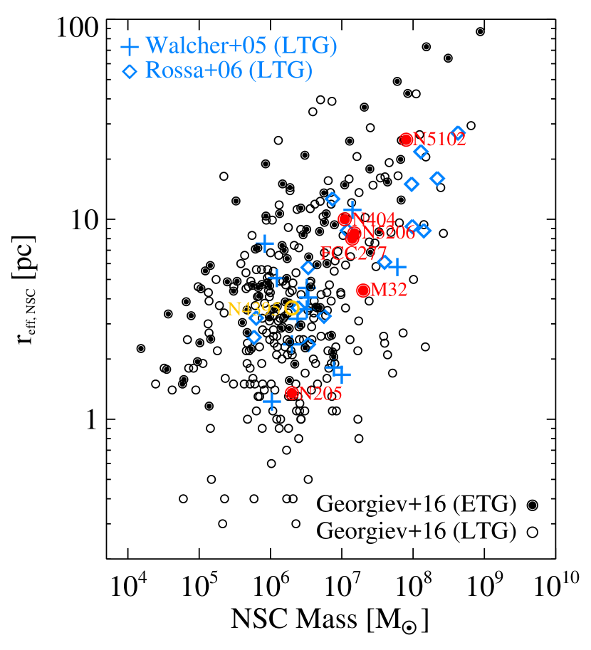
Figure 9.— Mass vs. size for NSCs. Our dynamical mass determinations plus that of NGC 404 Nguyen et al. (2017) are shown in red (dots + outer circles); these are the only dynamically determined NSC masses in early-type galaxies (ETGs). These are compared to photometric estimates from Georgiev et al. (2016) plotted both in black circles with central dots for ETGs and in black open circles for late-type galaxies (LTGs). LTG NSCs with the dynamical M/L estimates from Walcher et al. (2005) (late-type spirals) and the spectroscopic M/L estimates Rossa et al. (2006) (Sa-Sbc) are plotted in blue pluses and diamonds, respectively. We also add the dynamical M/L estimate for LTG NSC of NGC 4395 (den Brok et al., 2015) in yellow open circle and ETG NSC of FCC 277 (Lyubenova et al., 2013) in the same notation of this work NSCs.

To calculate the effective radii ($r_{\rm eff}$) of the multiple components NSCs in NGC 5102 and NGC 5206, we integrate the two components together to get an effective radius of $0\farcs 5$ (8 pc) for NGC 5206 and $1\farcs 6$ (26 pc) for NGC 5102. In Figure 9, we compare the sizes and dynamical masses of our ETG NSCs to previous measurements in other galaxies. Most of the previous measurements are photometric mass estimates taken from Georgiev et al. (2016). The dynamical M/L estimates are taken from Walcher et al. (2005) for LTGs, Lyubenova et al. (2013) for FCC 277, den Brok et al. (2015) for NGC 4395, Nguyen et al. (2017) for NGC 404, and the spectroscopic M/L estimates are taken from Rossa et al. (2006) for LTGs; we note here that our data are the first sample of dynamical NSC masses measured in ETGs. We find that all four of our NSCs fall within the existing distribution in the size-mass plane, with M32 and NGC 205 being on the compact side of the distribution.

7.2. Uncertainties on NSC Mass Estimates

For the quoted errors in the NSC masses shown in Table 7, we take the 3$\sigma$ errors on the mass scaling factors, and combine these in quadrature with uncertainties in the total luminosity of the NSCs to provide a conservative error estimate. The uncertainty in the total luminosity of the NSC (which comes from how much of the center is considered to be part of the NSC) ends up being the dominant error. The total fractional errors range between 11% and 21%. In addition to these errors, we consider the systematic error on the mass estimates from using different color–M/L relations. We find that the maximum differences are $<$12%, given that these are below the quoted uncertainties in all cases, we don’t quote separate systematic errors.

7.3. Structural Complexity and NSC formation

The NSCs of NGC 5102 and NGC 5206 have complex morphologies, made up of multiple components, while NGC 205 also shows clear color gradients within the nucleus. A similarly complex structure has also been seen in the NSC of nearby ETG NGC 404, where a central light excess in the central 0$\farcs$2 (3 pc) appears to be counter-rotating relative to the rest of the NSC (Seth et al., 2010) and has an age of $\sim$1 Gyr (Nguyen et al., 2017). The sizes of NSCs in spirals also change with wavelength, with bluer bands having smaller sizes and being more flattened, suggesting young populations are concentrated near the center (Seth et al., 2006; Georgiev & Böker, 2014; Carson et al., 2015). In NGC 5102, the central component dominates the light within the central 0$\farcs$2 (3 pc), while in NGC 5206, the central component dominates the light out to 0$\farcs$5 (8 pc). However, it is challenging to determine if these in fact are distinct components. In both NSCs the color gets bluer near the center, suggesting a morphology similar to that seen in the late-type NSCs. In NGC 5102, the outer component is somewhat more flattened, and has an elevated $V/\sigma$ value suggesting that it may be more strongly rotating than the inner component. In NGC 5206, both components have similar flattening and position angles, and no clear rotation kinematic differences are seen.

As NSCs have complex stellar populations, it is not surprising that their morphology may also be complex. These multiple components are likely linked to their formation history. In particular, the central bluer/younger components seen in 3/4 of our clusters strongly argue for in situ star formation, as in-spiraling clusters are expect to be tidally disrupted in the outskirts of any pre-existing cluster (e.g., Antonini, 2013). The gas required for in-situ star formation could be funneled into the nucleus by dynamical resonances in the galaxy disk (e.g., Schinnerer et al., 2003), or be produced within the NSC by stellar winds (Bailey, 1980) or collisions (Leigh et al., 2016). The large $r_{\rm eff}=32$ pc, high-mass fraction (1% of total galaxy mass) outer component in NGC 5102 may also be akin to the extra-light components expected to be formed from gas inflows during mergers (Hopkins et al., 2009). Regardless of the source of the gas, it is clear that NSCs in ETGs frequently host younger stellar populations within their centers, similar to late-type NSCs.

8. Discussion

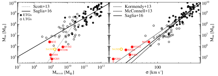
Figure 10.— Our four low-mass early-type galaxies in context of the $M_{\rm BH}$–$M_{\rm Bulge}$ (left) and $M_{\rm BH}$–$\sigma$ (right) scaling relations. The data of both early-type galaxies (ETGs, black dots with open circles) and late-type galaxies (black open circles) are taken from the compilation of Saglia et al. (2016). The dotted-, dashed-, long dashed-, and solid-lines indicate their linear best-fit in $\log$ scale of the relations from Scott et al. (2013); McConnell & Ma (2013); Kormendy & Ho (2013), and Saglia et al. (2016) for early-type galaxies (LTGs), respectively. The BH masses of M32, NGC 5102, and NGC 5206 and 3$\sigma$ upper limit mass of NGC 205 with the downward arrow are plotted in red dots + open circles as in the legend. We also add BHs with dynamical masses below $10^{6}$$M_{\odot}$, including the dwarf AGN late-type galaxy NGC 4395 (yellow open circle; den Brok et al., 2015) and early-type galaxy NGC 404 (Nguyen et al., 2017).

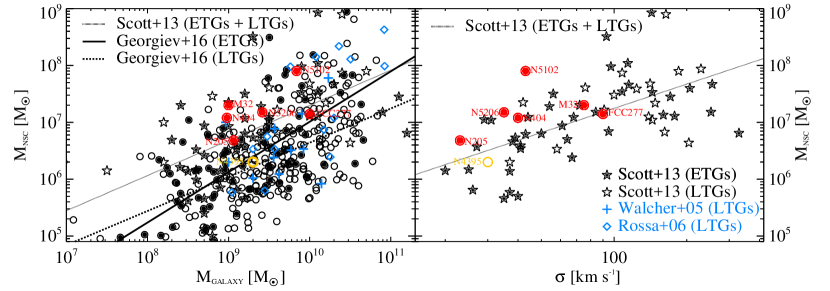
Figure 11.— Our four galaxies in context of the $M_{\rm NSC}$–galaxy mass (left) and $M_{\rm NSC}$–$\sigma$ (right) scaling relations. The data are taken from early-type galaxies (double stars) and late-type galaxies (open stars) Scott et al. (2013), and Georgiev et al. (2016) with early-type galaxies (ETGs) are plotted in black dots with circles, while late-type galaxies (LTGs) are plotted in open circles; and their corresponding linear best-fit in $\log$ scale. We note that the Scott et al. (2013) linear relation has been fit to the sample of both early-type (solid line) galaxies and late-type galaxies (dashed line). The M32, NGC 205, NGC 5102, and NGC 5206 NSCs are shown in color dots with circles as in the legend. We also add two more NSCs including of late-type galaxy NGC 4395 (den Brok et al., 2015) and early-type galaxy NGC 404 (Nguyen et al., 2017). NSCs have dynamical or spectroscopic M/L estimates from Walcher et al. (2005) (late-type spirals) and Rossa et al. (2006) (Sa-Sbc) are plotted in gray pluses and diamonds, respectively. We also add the dynamical estimate of the ETG NSC of FCC 277 (Lyubenova et al., 2013) in the same notation of this work NSCs. The total stellar of FCC 277 was estimated assuming its $B$–band absolute magnitude of $-17.78$ (http://leda.univ-lyon1.fr/search.html) and M/L${}_{B}\sim 5.0$ ($M_{\odot}$/$L_{\odot}$) at the highest $3\sigma$ of its Schwarzschild dynamical estimate in HST/ACS z–band (Lyubenova et al., 2013).

8.1. BH demographics

We have dynamically constrained the BH masses of M32, NGC 205, NGC 5102, and NGC 5206. While we find no evidence of a BH in NGC 205 (our 3$\sigma$ upper limit is $7\times 10^{4}$$M_{\odot}$), we detect BHs in the other three systems. Two of these best-fit BHs are below 10⁶$M_{\odot}$, in NGC 5206 ($4.7\times 10^{5}$$M_{\odot}$) and in NGC 5102 ($8.8\times 10^{5}$$M_{\odot}$). This doubles the previous sample of BHs with dynamical constraints placing them below 10⁶ $M_{\odot}$; the previous two were found in late-type spiral NGC 4395 (den Brok et al., 2015) and the accreting BH in NGC 404 (Nguyen et al., 2017). This adds significantly to the evidence that $\lesssim$$10^{6}$$M_{\odot}$ BHs do inhabit the nuclei of low-mass galaxies (see also Reines & Volonteri, 2015).

Combining our results with the accretion evidence for a BH in NGC 404 (Nguyen et al., 2017), we can make a measurement of the fraction of the nearest ETGs that host BHs. These five galaxies have total stellar masses between $5\times 10^{8}$$M_{\odot}$–$10\times 10^{9}$$M_{\odot}$. This sample represents a complete, volume limited sample of ETGs in this mass range, and thus forms a small but unbiased sample of ETGs (Section 3). Most of the galaxies are satellite galaxies, with only NGC 404 being isolated, thus these represent only group and isolated environments. With four of five of these galaxies now having strong evidence for central BHs, we measure an occupation fraction of 80% over this stellar mass range.

We can directly compare this to the occupation fraction estimates from the AMUSE survey of X-ray nuclei in ETGs (Gallo et al., 2008; Miller et al., 2015). Of the 57 galaxies observed in the mass range of our ETGs, only 9 (16%) have detected X-rays sources, however, modeling of the X-ray luminosity function suggests occupation fraction of 30–100% for these galaxies (Miller et al., 2015). Thus both dynamical and accretion evidences points to high mass occupation fraction for ETGs down to $\sim$10⁹ M_⊙.

The high occupation fraction we find here can be used to constrain the seed formation mechanism of BHs in the early Universe. Our result appears to be more consistent with the scenario where BH seeds are formed from the remnants of the first generation of massive stars (e.g., Population III stars (light seeds), Volonteri et al., 2008; Volonteri, 2010; Greene, 2012; Reines & Comastri, 2016), rather than heavier seeds. More specifically, the 80% observed occupation fraction is consistent with the semi-analytic model predictions at $z=0$ for light seeds as a function of velocity dispersion (Volonteri et al., 2008; van Wassenhove et al., 2010). A more recent semi-analytic prediction predicts a significantly lower BH occupation of $\sim$20% in our mass range for the low-mass seed scenario Antonini et al. (2015a). This study also breaks down the prediction by galaxy type, with even lower occupation fraction expected in similar mass LTGs. We note that our measurements apply only to ETGs, which make up a minority of galaxies at the stellar masses probed (e.g., Blanton et al., 2005).

Our BH masses are also consistent with their formation from runaway tidal capture of NSC stars, a scenario outlined by Stone et al. (2017). Stone et al. (2017) find that this runaway tidal capture processes requires dense NSCs that are typically found only in galaxies with $\sigma\gtrsim 35$ km s^-1. For sufficiently dense NSCs (in higher dispersion galaxies), the runaway tidal encounters supplies mass for the BH seed to grow, and this growth is larger for higher dispersion galaxies. Over a Hubble time, this BH growth saturates at a specific mass. Using their equation 37, we find saturation masses of $\sim$$6.5\times 10^{5}$$M_{\odot}$, $\sim$$5\times 10^{5}$$M_{\odot}$, $\sim$$1\times 10^{6}$$M_{\odot}$ for NGC 5102, NGC 5206, and M32, respectively using the velocity dispersions are estimated in Section 8.2. These BH masses are within a factor of $\sim$2 of the BH masses we dynamically measure in Section 6.1. NGC 205 and NGC 404 both fall below the threshold dispersion where runaway tidal growth is expected, and our upper mass limits in these galaxies are therefore also consistent with this scenario.

Additional constraints on the occupation fraction in a wider range of galaxy types are possible in the local volume, and in future work we plan to provide additional constraints using existing data on LTGs with both stellar kinematics using Gemini/NIFS or VLT/SINFONI and upcoming gas kinematic data from ALMA.

8.2. BH Mass Scaling Relations

We examine our best-fit BH masses in the context of scaling relations including $M_{\rm BH}$–$M_{\rm Bulge}$ and $M_{\rm BH}$–$\sigma$ (Kormendy & Ho, 2013; McConnell & Ma, 2013; Saglia et al., 2016) for ETGs. Since our dynamical constraints suggest $\gamma\sim 1$, and we do not have direct dynamical measurements of the bulge masses, we assume population based masses for the bulge components here for all four galaxies; these are listed in Column 12 of Table 5.

We note that we assume the galactic bulges are comprised of all two (NGC 205 and M32) and three (NGC 5102 and NGC 5206) Sérsic components. Kormendy & Ho (2013), McConnell & Ma (2013), and Saglia et al. (2016) report the bulge mass and luminosity of M32 are $\sim$$4.5\times 10^{8}$$M_{\odot}$ and $\sim$$4\times 10^{8}$$L_{\odot}$ ($M_{V}=-16.64$), while our estimates of mass and luminosity from F814W are $M_{\rm Bulge}$ $\sim 8.2\times 10^{8}$$M_{\odot}$ and $L_{\rm Bulge}$ $\sim 4.5\times 10^{8}$$L_{\odot}$; these are consistent with Graham & Spitler (2009); Kormendy & Bender (2009) estimated in $I$–band. For NGC 205, McConnachie (2012) reports a total luminosity of $M_{V}=-16.5$ ($3\times 10^{8}$$L_{\odot}$) and Angus et al. (2016) simulation gives a mass of $4.0\times 10^{8}$$M_{\odot}$. We find a consistent luminosity but higher mass for the bulge of $6.5\times 10^{8}$$M_{\odot}$ from F814W HST data.

Figure 10 shows the best-fit BH mass of M32 is within the scatter of the $M_{\rm BH}$–$M_{\rm Bulge}$ relations of Kormendy & Ho (2013), McConnell & Ma (2013), and Saglia et al. (2016). However, the best-fit BHs masses of NGC 205, NGC 5102, and NGC 5206 clearly fall below these $M_{\rm BH}$–$M_{\rm Bulge}$ relations by 1-2 orders of magnitude. Combined with other recent work on BH mass measurements in low-mass systems, e.g., NGC 404 (Nguyen et al., 2017), NGC 4395 (den Brok et al., 2015), RGG118 (Baldassare et al., 2015), Pox52 (Barth et al., 2004; Thornton et al., 2008), an increasing number of galaxies appear to fall below the BH mass vs. bulge mass relationship extrapolated from massive ETGs to the low-mass regime. This suggests that the $M_{\rm BH}$–$M_{\rm Bulge}$ relationship may steepen as suggested by Scott et al. (2013) for low-mass systems with bulge mass $<$$2\times 10^{10}$$M_{\odot}$. Alternatively, the scaling relations may just break down at these masses, with significant scatter to lower masses as also seen in the megamaser BH measurements in spiral galaxies (Läsker et al., 2016a; Greene et al., 2016). We note that this increased scatter may occur at bulge masses where the occupation fraction also drops below unity.

Next, we explore these BHs in the context of the $M_{\rm BH}$–$\sigma$ scaling correlation. While typically the dispersion used is that estimated within the effective radius, we do not have this information for all of our galaxies. For M32 and NGC 205, the $\sigma_{e}$ have been measured by Ho et al. (2009) who measure the dispersions of $72.1\pm 1.9$ km s^-1and $23.3\pm 3.7$ km s^-1 in a $2\arcsec\times 4\arcsec$ aperture, respectively. To estimate the central velocity dispersions of NGC 5102 and NGC 5206, we co-add all the spectra in the FOV of 1$\farcs$5 and fit the resulting single spectrum with pPXF for velocity dispersions. This gives dispersions of $42.3\pm 1.1$ km s^-1 for NGC 5102 and $35.4\pm 1.0$ km s^-1 for NGC 5206.

8.3. Possibility of Collections of Dark Remnants

Recent work has suggested that mass segregation of stellar mass BHs can occur on timescales well below the relaxation time (Bianchini et al., 2017), significantly enhancing the central M/L of globular clusters. An enhancement of M/L is in fact seen in the globular cluster M15 (den Brok et al., 2014a). This leads to the possibility that a significant number of stellar mass BHs could collect at the center of NSCs, leading to a false detection of a massive BH. We note that the current simulations are of much lower mass systems than the massive NSCs we discuss here, and that significant uncertainties exist on how many BHs would segregate and be retained during this process. Nonetheless, we can get a sense of the maximum dark mass that can plausibly be accumulated by stellar remnants. For a Solar metallicity population with a standard Kroupa IMF, $\sim$4% of the mass of the cluster will turn into stellar mass BHs (Shanahan & Gieles, 2015). This represents a maximum mass fraction of the NSCs that could be concentrated at the center with the retention fraction of BHs likely being much lower than this. The fraction of the NSC mass found in the BH in M32, NGC 205, NGC 5102, and NGC 5206 are 13%, $<$3.5%, 1.1%, and 3.3% of their NSC masses, respectively. Therefore, based on the mass fractions, apart from M32, a collection of dark remnants is a possibility.

We can also evaluate stellar relaxation times ($t_{\rm relaxation}$) of these nuclei at the effective radii of their NSCs using the following equation (Bahcall & Wolf, 1977; Valluri et al., 2005):

$$t_{\rm relaxation}\simeq(1.4\times 10^{8})\sigma_{20}^{3}\rho_{5}^{-1}(\ln\Lambda_{10})^{-1}~{}({\rm yrs})$$ (1)

where $\sigma_{20}=\sigma_{\star}/20$ km s^-1, $\rho_{5}=(\rho_{\rm g,\;dyn.})/10^{5}$ $M_{\odot}$ pc^-3, $\ln\Lambda_{10}=\ln\Lambda/10$, and $\ln\Lambda=10$. $\sigma_{\star}$ is the stellar dispersion estimated in Section 8.2, and the mass densities $\rho_{\rm g,\;dyn}$ are estimated at the effective radii of NSCs. These mass densities and relaxation times are provided in Table 7. Our estimated relaxation times for the BH detections are long (6.8-38 Gyr), while in NGC 205 (the one source without a BH detection), the relaxation time is quite short (0.58 Gyr). The fact that we detect no BH in this shortest relaxation time system (as well as the tight upper limit on the mass of the M33 BH Gebhardt et al., 2001) argues against the detected BHs being collections of remnants. However, more realistic simulations are required to evaluate whether significant fractions of the NSC BHs can really be mass segregated and retained.

8.4. NSC Masses and Scaling Relations

Our dynamical mass measurements of the four NSCs in this work along with the measurement of NGC 404 NSC (Seth et al., 2010; Nguyen et al., 2017) and FCC 277 (Lyubenova et al., 2013) are the first six dynamical mass measurements of NSCs in ETGs. These NSC masses are plotted against the mass and dispersion of galaxies in Figure 11.

Comparing our dynamical NSC masses to the galaxy stellar masses and dispersions, we find that they are within the scatter of the previous (mostly photometric) NSC mass measurements. However, almost all of the dynamical measurements lie on or above previous relations, with NGC 5102 the highest mass outlier. The closest previously published relations are those presented in (Scott et al., 2013). The (Georgiev et al., 2016) NSC–galaxy mass relation for ETGs lies below all 6 dynamical measurements.

The ratios between the NSCs masses and their host bulges/galaxies masses are $\sim$1.7%, 0.2%, 1.1%, 0.7%, and $<$1.5% for M32, NGC 205, NGC 5102, NGC 5206, and NGC 404 (Nguyen et al., 2017) respectively. Apart from NGC 205, these NSCs are more massive than the typical $\sim$0.3% mass fraction for NSCs seen in ETGs with similar stellar mass in the Virgo cluster (Côté et al., 2006; Spengler et al., 2017). A trend towards higher mass NSCs in lower mass galaxies was suggested by Graham & Spitler (2009) and is verified for ETGs in recent work (Spengler et al., 2017); based on the Graham & Spitler (2009) relation a mass fraction of $\sim$1% is expected for our sample galaxies. The high masses and mass fractions inferred here might be a sign that the relation of NSC to galaxy mass changes outside cluster environments, as might be expected based on the increased availability of gas to accrete to the present day.

8.5. Relative Formation Between NSCs and BHs

As discussed in the introduction, the relationship between NSCs and BHs is not yet clear. Our galaxies add significantly to the sample of galaxies where we have mass measurements for both the BH and NSC. Our three BH detections have a $M_{\rm BH}$/$M_{\rm NSC}$ ratio between $10^{-2}$ and $0.3$. We plot these against the galaxy mass and NSC mass in Figure 12. The $M_{\rm BH}$/$M_{\rm NSC}$ ratio in our galaxies is consistent with galaxies like the MW (e.g., Schödel et al., 2014), and previous measurements of Ultracompact Dwarfs (UCDs) (Seth et al., 2014; Ahn et al., 2017), where just the inner component of the UCD is assumed to be the remnant NSC. However, the lack of NSCs in massive ETGs clearly separates these from our sample (Neumayer & Walcher, 2012). On the other hand, for spiral galaxies with upper limits on the BHs (Neumayer & Walcher, 2012), our NGC 205 limit joins previous measurements constraining the BH mass to be at most $10^{-2}$ to $10^{-3}$ that of the NSC. Even amongst the sample where both BH and NSC are found, there is a scatter of $\sim$3 orders of magnitude at similar NSC mass. This wide range of $M_{\rm BH}$/$M_{\rm NSC}$ ratios suggests that NSC and BH formation must not always be tightly linked.

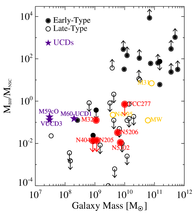
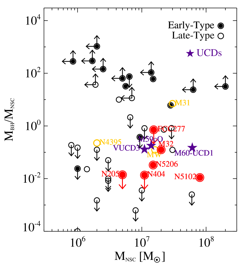
Figure 12.— Ratio of the BH and NSC mass against their host-galaxy stellar mass (left) and their NSC dynamical masses based on dynamical measurements of M/L_dyn. (right). Original data with dynamical measurements are shown with early- (black dots), late-type (gray dots) galaxies, and current BH mass measurements of UCDs (black stars) are taken from Neumayer & Walcher (2012), Graham & Spitler (2009), Lyubenova et al. (FCC 277; 2013), Seth et al. (M60-UCD1; 2014), and Ahn et al. (VUCD3 and M59cO; 2017). The upward/downward arrows are used for galaxies with lower/upper limits of BH and NSC masses. We note that the for the UCD NSC masses, we plot only the mass of their inner components.

8.6. Relation of NSCs to UCDs

The infall and ongoing stripping of the Sagittarius dwarf spheroidal galaxy shows that nuclei similar to those we sample here can be stripped of their host galaxies (e.g., Monaco et al., 2005). Our NSCs clearly overlap with the radii and mass distribution of UCDs (Norris et al., 2014), and some of these UCDs may be stripped galaxy nuclei (e.g., Pfeffer et al., 2014). UCDs typically have higher than expected integrated dispersion (e.g., Haşegan et al., 2005). Specifically, virial mass estimates based on these dispersions give $M/L$s higher than expected from their stellar populations – these can be interpreted as indirect evidence for massive BHs (Mieske et al., 2013), as would be expected if UCDs were tidally stripped NSCs. The presence of these BHs with mass fractions above 10% has been verified in a few massive UCDs ($>$$10^{7}$$M_{\odot}$) using resolved kinematic measurements (Seth et al., 2014; Ahn et al., 2017). We can examine the apparent increase in $M/L$ of our galaxies if we were to ignore the BHs by looking at the no BH model $M/L$s; these are inflated by 4–10.0% in our three galaxies with detected BHs; this is smaller than the effect observed in known UCDs due to the smaller mass fractions of the BHs (1–13%) in these systems. We note that the UCDs are often observed to have multiple components, thus the NSCs may make up only a fraction their total mass, suggesting even lower BH mass fractions if these galaxies were to be stripped.

9. Conclusions $\&$ Future Prospects

9.1. Conclusions

We have examined the nuclear morphology and kinematics of a sample of four ETGs with stellar masses of $10^{9}-10^{10}$$M_{\odot}$ using adaptive optics Gemini/NIFS and VLT/SINFONI spectroscopic data and HST imaging. We use HST data to estimate the sizes, masses, and luminosities of their NSCs. Using dynamical modeling of the spectroscopic data, we constrain the mass of their central BHs and NSCs. Our primary findings are as follows.

1. Our dynamical models yield significant detection of central BHs in M32, NGC 5102, and NGC 5206 and an upper limit in NGC 205. The NGC 205 upper limit and M32 BH masses are consistent with previous measurements.

2. We present the first dynamical measurements of the central BH masses in NGC 5102 and NGC 5206. Both BHs have masses below 1 million $M_{\odot}$, thus doubling the number of dynamical measurements of sub-million solar-mass BHs (den Brok et al., 2015; Nguyen et al., 2017).

3. Including our recent work on the BH in NGC 404 (Nguyen et al., 2017), we find that the fraction of $10^{9}-10^{10}$$M_{\odot}$ ($\sigma_{\star}=$20 km s^-1 to 70 km s^-1) ETGs that host central BHs is at least 80% (4/5 with detected BHs). These galaxies represent a volume limited sample of ETGs in this mass range. This rather high occupation fraction suggests that the early universe produced an abundance of BH seeds, favoring a scenario where BH seeds formed from the population III stars (e.g., Volonteri, 2010). Our BH masses are also consistent with growth by runaway tidal encounters (Stone et al., 2017).

4. The effective radii of the NSCs are $\sim$2–26 pc. The NSC SB profiles of NGC 205 and M32 are both fit well by a single Sérsic function, but the NSCs of NGC 5102 and NGC 5206 appear to have more complicated nuclear structures requiring two Sérsic components.

5. The high-quality ($\sim$0$\farcs$1 resolution) kinematics of M32 and NGC 5102 show strong rotation ($V/\sigma\gtrsim 0.7$), while NGC 205 and NGC 5206 have less significant rotation ($V/\sigma\sim 0.3$).

6. We measure the masses of the NSCs in all four galaxies dynamically, some of the first dynamical mass estimates of ETG NSCs. Their dynamical masses range from $0.2\times 10^{7}$$M_{\odot}$ to $7.3\times 10^{7}$$M_{\odot}$. These NSC masses are higher than the typical ETGs of similar galaxy mass in the Virgo and Fornax clusters, suggesting a possible environmental dependence on the NSC mass.

7. The BHs and NSCs in these galaxies appear to follow the $M_{\rm BH}$–$\sigma$ and $M_{\rm NSC}$–$\sigma$ relations. Their BHs fall below the bulge mass/total stellar mass–BH mass relations, while their NSCs are located above similar relations.

9.2. Future Prospects

Our dynamical modeling using high resolution stellar kinematics from NIFS and SINFONI spectroscopy confirm the existence of an BH in M32 and put an upper limit on the NGC 205’s BH mass. We also measure the masses of BHs in NGC 5102 and NGC 5206 for the first time. However, we model these BH masses assuming a constant M/L or the B03 and R15 color–M/L relations. Although the assumption of a constant M/L is good for M32, the nuclei of NGC 205, NGC 5102, and NGC 5206 show the clear spatial population variations and hence their nuclear M/Ls. We will model these M/L variations using new STIS data obtained this year using the techniques we developed in Nguyen et al. (2017). This data will enable stellar population synthesis modeling on the same 0$\farcs$05 scale as our kinematic observations. With this information we can significantly reduce the uncertainties in the stellar mass profiles and the resulting BH mass estimates. Moreover, our upcoming ALMA data will also be able to allow us to measure the central BH masses using cold gas kinematic models of the circumnuclear gas disk (CND) within the nuclei of a variety Hubble type, nearby, and low-mass galaxy sample. This larger and high quality data sample will provide a more precise, complete, and unbiased occupation fraction dynamically.

Appendix A Measurement of the NGC 5102 Nucleus $(B-V)_{0}$ Color Profile

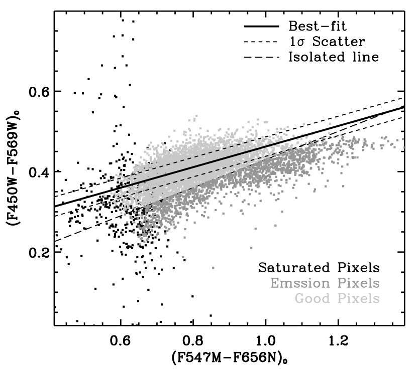
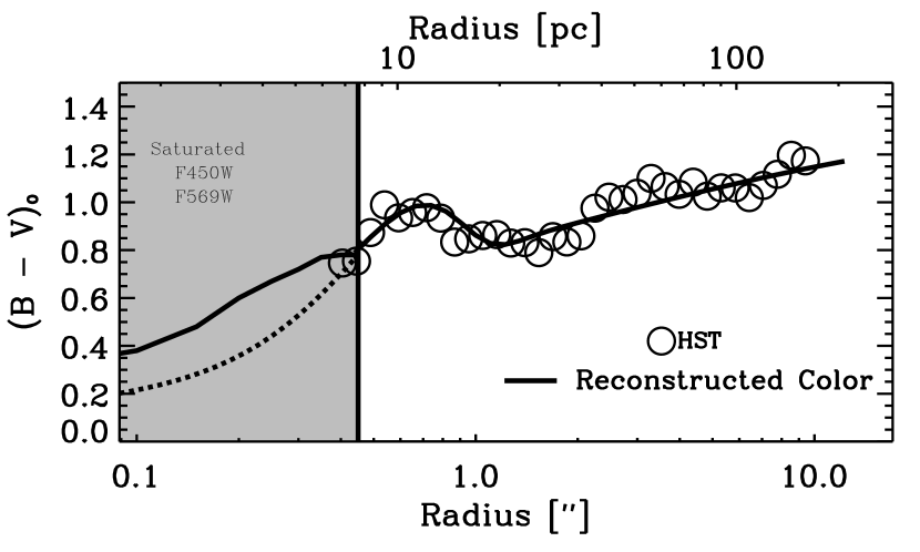
Figure 13.— Top panel: F450W–F569W vs. F547M–F656N color–color correlation for NGC 5102 nucleus. Black dots are the saturated pixels within $0\farcs 4$ in F450W and F569W. Gray dots are the pixels that are possibly contaminated by H${\alpha}$ emission in F656N band. White-gray dots are pixels outside $0\farcs 4$, which are used for the fit. The solid line is the best-fit of (F450W–F569W)₀ vs. (F547M–F656N)₀ relation, while the dashed lines represent 1$\sigma$ scatter of the best-fit. The long-dashed line shows the isolation criterion of H$\alpha$, (F547M–F656N)${}_{0}\gtrsim 2.5\times$(F450W–F569W)₀. Bottom panel: the $(B-V)_{0}$ color profile, which is inferred from the HST photometric transformation from WFPC2 $\rightarrow$ $BVRI$ (Sirianni et al., 2005). Open circles are the HST data outside $0\farcs 4$ and the gray region is the saturated HST data within $0\farcs 4$. The solid line is the best-fit model of $(B-V)_{\rm 0}$ colors, while the dashed line is the original saturated color.

We determine $(B-V)_{0}$ colors of NGC 5102 inside the radii of $0\farcs 4$ from F450W–F569W WFPC2 data. However, these data are saturated at the center. We can use the F547M–F656N data to predict the central $(B-V)_{0}$ colors where does not appear to be strong H${\alpha}$ emission. The upper panel of Figure 13 shows the scheme that we use to explore the $\lesssim$$0\farcs 4$ $(B-V)_{0}$ colors. First, we create the (F450W–F569W)₀ and (F547M–F656N)₀ color maps with PSF cross convolution and Galactic extinction correction in each band. Second, we get rid of all the colors with saturated pixels from F450W and F569W in both (F450W–F569W)₀ and (F547M–F656N)₀ maps (balck dots). The pixels with possible contaminated by H${\alpha}$ emission in F656N band were also eliminated based on the criterion of (F547M–F656N)${}_{0}\gtrsim 2.5\times$(F450W–F569W)₀ (gray dots under the long-dashed line). All the good pixels are presented in white-gray dots. Third, we use these good pixels of colors to fit the linear correlation between (F450W–F569W)₀ and (F547M–F656N)₀. The best-fit is presented by the solid black line, while the scatter by 1$\sigma$ of the fit is shown by the dashed black lines. The central (F450W–F569W)₀ color profile is inferred from this (F450W–F569W)₀–(F547M–F656N)₀ correlation.

We transform the (F450W–F569W)₀ colors into the $(B-V)_{\rm 0}$ colors using the HST photometric transformation from WFPC2 $\rightarrow$ $BVRI$ (Sirianni et al., 2005). The $(B-V)_{\rm 0}$ colors include the central region ($\lesssim$$0\farcs 4$) that is shown in the lower panel of Figure 13. We plot the $(B-V)_{\rm 0}$ color profile of the outer part with radii $>$$0\farcs 4$ from $B$– (transformed from HST F450W) and $V$–band (transformed from HST F569W) (open circles for data, and black solid line for the best-fit 1D model), while the saturated $(B-V)_{\rm 0}$ within the radii $r\lesssim 0\farcs 4$ is plotted in gray region with 1D profile is shown black dotted line. The best-fit reconstruction of $(B-V)_{\rm 0}$ is presented in black solid line. This new color profile results a smaller mass of the NGC 5102 NSC of $M_{\rm NSC}$ $=(8.0\pm 1.3)\times 10^{7}$$M_{\odot}$, $\sim$23% smaller than its mass with the assumption of constant $(V-I)_{\rm 0}\sim 1$ in the $\lesssim$$1\arcsec$ region inferred from the ground-based observation (CGS), but totally consistent to the dynamical estimate in Table 7. Also, we note that we will use this $(B-V)_{\rm 0}$ color profile to model the mass model for NGC 5102 throughout this paper.

Appendix B Kinematics Tables, MGE Models, and JAM’s Results

We make the full kinematic data set available in Table 8, Table 9, and Table 10 of NGC 205, NGC 5102, and NGC 5206 for use in future studies respectively. Table 11 of MGE models of four galaxies used in JAM models (Section 6) are presented in this section as well. Also, the complete results of JAM models indicate for its systemic uncertainties are shown in Table 13.

Table 8Gemini/NIFS Kinematic Data of the NGC 205 Nucleus

$\Delta$R.A. ($\arcsec$)	$\Delta$Decl. ($\arcsec$)	$V_{\rm r}$ (km s-1)	$\sigma$ (km s-1)
…	…	…	…
$-$0.10	$-$0.09	$-$263.33 $\pm$ 3.06	15.26 $\pm$ 2.20
$-$0.10	0.01	$-$269.34 $\pm$ 1.10	15.63 $\pm$ 0.98
$-$0.15	$-$0.04	$-$267.32 $\pm$ 2.69	16.34 $\pm$ 2.65
…	…	…	…

Table 9VLT/SINFONI Kinematic Data of the NGC 5102 Nucleus

$\Delta$R.A. ($\arcsec$)	$\Delta$Decl. ($\arcsec$)	$V_{\rm r}$ (km s-1)	$\sigma$ (km s-1)
…	…	…	…
0.02	$-$0.02	492.93 $\pm$ 1.29	56.53 $\pm$ 2.84
0.00	0.03	490.75 $\pm$ 1.42	56.04 $\pm$ 3.26
$-$0.03	$-$0.04	492.97 $\pm$ 1.28	52.16 $\pm$ 2.36
…	…	…	…

Table 10VLT/SINFONI Kinematic Data of the NGC 5206 Nucleus

$\Delta$R.A. ($\arcsec$)	$\Delta$Decl. ($\arcsec$)	$V_{\rm r}$ (km s-1)	$\sigma$ (km s-1)
…	…	…	…
0.01	0.02	610.18 $\pm$ 2.55	44.85 $\pm$ 3.46
0.01	$-$0.03	608.95 $\pm$ 2.39	44.57 $\pm$ 2.76
0.01	0.07	607.90 $\pm$ 2.07	44.24 $\pm$ 2.66
…	…	…	…

Table 11Luminosity and Mass MGE Models Using in Dynamical Modeling

		M32
Mass	Light	$\sigma$	$a/b$	P.A.
($M_{\odot}$/${\rm pc^{2}}$)	($L_{\odot}$/${\rm pc^{2}}$)	(′′)		(∘)
(1)	(2)	(3)	(4)	(5)
5.01	4.74	$-$2.76	0.75	$-$25.0
5.38	5.11	$-$2.25	0.75	$-$25.0
5.64	5.37	$-$1.78	0.75	$-$25.0
5.80	5.53	$-$1.34	0.75	$-$25.0
5.85	5.58	$-$0.94	0.75	$-$25.0
5.79	5.52	$-$0.57	0.75	$-$25.0
5.62	5.35	$-$0.23	0.75	$-$25.0
5.34	5.07	0.095	0.79	$-$25.0
4.93	4.66	0.398	0.79	$-$25.0
4.41	4.14	0.680	0.79	$-$25.0
3.77	3.50	0.946	0.79	$-$25.0
3.32	3.06	1.030	0.79	$-$25.0
3.00	2.73	1.195	0.79	$-$25.0
3.54	3.28	1.382	0.79	$-$25.0
3.19	2.92	1.611	0.79	$-$25.0
2.87	2.60	1.775	0.79	$-$25.0
2.71	2.44	1.907	0.79	$-$25.0
2.46	2.19	2.028	0.79	$-$25.0
		NGC 205
Mass	Light	$\sigma$	$(a/b)$	P.A.
($M_{\odot}$/${\rm pc^{2}}$)	($L_{\odot}$/${\rm pc^{2}}$)	(′′)		(∘)
(1)	(2)	(3)	(4)	(5)
4.87	4.58	$-$1.75	0.95	$-$40.4
4.73	4.44	$-$1.50	0.95	$-$40.4
5.23	4.94	$-$1.15	0.95	$-$40.4
4.38	4.09	$-$0.92	0.95	$-$40.4
4.93	4.64	$-$0.68	0.95	$-$40.4
4.84	4.55	$-$0.23	0.95	$-$40.4
4.36	4.07	$-$0.00	0.95	$-$40.4
3.64	3.35	0.201	0.95	$-$40.4
3.62	3.33	0.871	0.90	$-$40.4
3.02	2.74	1.165	0.90	$-$40.4

Table 12Luminosity and Mass MGE Models Using in Dynamical Modeling (continue of Table 11)

		NGC 5102
Mass	Light	$\sigma$	$(a/b)$	P.A.
($M_{\odot}$/${\rm pc^{2}}$)	($L_{\odot}$/${\rm pc^{2}}$)	(′′)		(∘)
(1)	(2)	(3)	(4)	(5)
6.95	5.81	$-$1.28	0.68	50.5
6.70	5.26	$-$1.11	0.68	50.5
5.94	4.50	$-$0.77	0.68	50.5
4.95	3.51	$-$0.40	0.68	50.5
4.89	4.05	$-$0.26	0.68	50.5
4.77	3.93	0.25	0.60	50.5
4.65	3.63	0.37	0.60	50.5
3.47	2.46	0.82	0.60	50.5
3.11	2.09	0.88	0.60	50.5
2.88	2.04	1.38	0.60	50.5
2.82	1.98	1.64	0.60	50.5
2.48	1.63	1.75	0.60	50.5
2.76	1.92	1.77	0.60	50.5
2.47	1.62	1.32	0.60	50.5
		NGC 5206
Mass	Light	$\sigma$	$(a/b)$	P.A.
($M_{\odot}$/${\rm pc^{2}}$)	($L_{\odot}$/${\rm pc^{2}}$)	(′′)		(∘)
(1)	(2)	(3)	(4)	(5)
5.60	5.49	$-$1.74	0.96	38.3
5.58	5.48	$-$1.20	0.96	38.3
5.43	5.33	$-$1.11	0.96	38.3
5.34	5.23	$-$0.78	0.96	38.3
4.16	4.06	$-$0.66	0.96	38.3
3.93	3.82	$-$0.41	0.96	38.3
3.83	3.72	$-$0.27	0.96	38.3
2.88	2.79	$-$0.16	0.96	38.3
2.98	2.88	$-$0.08	0.98	38.3
2.88	2.80	0.760	0.98	38.3
2.61	2.73	0.890	0.98	38.3
2.58	2.64	0.988	0.98	38.3
2.40	2.33	1.316	0.98	38.3
2.29	2.19	2.169	0.98	38.3

Table 13Jeans modeling results (full table)

Object	Filter	Color–M/L	$M_{\rm BH}$	$\beta_{\rm z}$	$\gamma$	$i$	Number of Bins	$\chi^{2}_{\rm r}$	$r_{g}$	$r_{g}$
			($M_{\odot}$)			(∘)			($\arcsec$)	(pc)
(1)	(2)	(3)	(4)	(5)	(6)	(7)	(8)	(9)	(10)	(11)
M32	F555WG	R15	$2.3^{+1.3}_{-1.5}\times 10^{6}$	$-0.25^{+0.35}_{-0.25}$	$1.05^{+0.20}_{-0.15}$	$74^{+12}_{-9}$	1354	1.35	0.455	1.81
	F555WD	R15	$2.5\times 10^{6}$	$-$0.25	1.05	74		1.39	0.403	1.60
	F814WG	B03	$2.0^{+0.5}_{-0.8}\times 10^{6}$	$-0.15^{+0.35}_{-0.35}$	$1.07^{+0.14}_{-0.10}$	$72^{+6}_{-6}$		1.31	0.337	1.35
	F814WG	Conts	$2.0^{+0.3}_{-1.0}\times 10^{6}$	$-0.20^{+0.40}_{-0.40}$	$1.03^{+0.17}_{-0.08}$	$70^{+4}_{-5}$		1.97	0.337	1.35
	F814WD	R15	$2.4\times 10^{6}$	$-$0.20	1.08	70		1.75	0.387	1.61
	F814WD	B03	$2.2\times 10^{6}$	$-$0.15	1.05	72		1.83	0.319	1.35
	F814WD	Conts	$2.1\times 10^{6}$	$-$0.20	1.03	70		2.04	0.303	1.35
NGC 205	F555WD	R15	$2.7\times 10^{4}$	0.27	1.07	60	256	1.33	0.070	0.30
	F555WG∗	R15	$2.1\times 10^{4}$	0.25	1.07	60		1.37	0.051	0.17
	F555WD∗	R15	$3.0^{+3.2}_{-3.0}\times 10^{4}$	$0.27^{+0.08}_{-0.18}$	$1.07^{+0.18}_{-0.20}$	$60^{+5}_{-8}$	197	1.37	0.074	0.35
	F814WD∗	B03	$2.0^{+4.0}_{-2.0}\times 10^{4}$	$0.25^{+0.06}_{-0.04}$	$1.09^{+0.07}_{-0.10}$	$66^{+4}_{-8}$		1.40	0.063	0.22
	F814WD∗	Const	$1.8^{+3.2}_{-1.8}\times 10^{4}$	$0.27^{+0.04}_{-0.06}$	$1.07^{+0.08}_{-0.07}$	$67^{+4}_{-7}$		2.51	0.060	0.20
NGC 5102	F547MG	B03	$7.0^{+10.0}_{-2.0}\times 10^{5}$	$0.25^{+0.08}_{-0.14}$	$1.13^{+0.03}_{-0.04}$	$76.5^{+8.5}_{-6.0}$	1017	1.23	0.056	0.89
	F547MG	Const	$6.0^{+9.0}_{-3.5}\times 10^{5}$	$0.09^{+0.08}_{-0.12}$	$1.08^{+0.03}_{-0.05}$	$72.5^{+5.5}_{-4.5}$		2.32	0.048	0.76
	F547MD	R15	$8.0\times 10^{5}$	0.15	1.15	71.5		1.57	0.070	1.20
	F547MD	B03	$7.5\times 10^{5}$	0.18	1.13	76.0		1.73	0.056	0.89
	F547MD	Const	$7.2\times 10^{5}$	0.13	1.08	72.5		2.92	0.048	0.82
NGC 5206	F555WG	R15	$5.1^{+2.3}_{-1.2}\times 10^{5}$	$0.28^{+0.07}_{-0.14}$	$1.08^{+0.20}_{-0.40}$	$43.5^{+4.0}_{-4.5}$	240	1.33	0.061	1.04
	F555WD	R15	$4.8\times 10^{5}$	0.28	1.08	43.5		1.36	0.071	1.21
	F814WG	B03	$2.4^{+1.1}_{-1.3}\times 10^{5}$	$0.27^{+0.04}_{-0.15}$	$1.10^{+0.05}_{-0.10}$	$41.0^{+2.5}_{-2.5}$		1.57	0.045	0.75
	F814WG	Const	$2.1^{+0.8}_{-1.4}\times 10^{5}$	$0.29^{+0.06}_{-0.04}$	$1.06^{+0.10}_{-0.05}$	$45.0^{+2.5}_{-1.5}$		2.41	0.038	0.65
	F814WD	R15	$4.5\times 10^{5}$	0.25	1.06	44.0		1.70	0.058	1.00
	F814WD	B03	$2.3\times 10^{5}$	0.27	1.10	41.0		1.66	0.045	0.75
	F814WD	Const	$2.0\times 10^{5}$	0.29	1.06	45.0		2.78	0.038	0.65

References

- Ahn et al. (2017) Ahn, C. P., Seth, A. C., den Brok, M., et al. 2017, ApJ, 839, 72
- Angus et al. (2016) Angus, G. W., Coppin, P., Gentile, G., & Diaferio, A. 2016, MNRAS, 462, 3221
- Antonini (2013) Antonini, F. 2013, ApJ, 763, 62
- Antonini et al. (2015a) Antonini, F., Barausse, E., & Silk, J. 2015a, ApJ, 812, 72
- Antonini et al. (2015b) —. 2015b, ApJ, 806, L8
- Avila et al. (2012) Avila, R. J., Hack, W. J., & STScI AstroDrizzle Team. 2012, in American Astronomical Society Meeting Abstracts, Vol. 220, American Astronomical Society Meeting Abstracts 220, #135.13
- Bahcall & Wolf (1977) Bahcall, J. N., & Wolf, R. A. 1977, ApJ, 216, 883
- Bailey (1980) Bailey, M. E. 1980, MNRAS, 191, 195
- Baldassare et al. (2015) Baldassare, V. F., Reines, A. E., Gallo, E., & Greene, J. E. 2015, ApJ, 809, L14
- Barth et al. (2004) Barth, A. J., Ho, L. C., Rutledge, R. E., & Sargent, W. L. W. 2004, ApJ, 607, 90
- Bell & de Jong (2001) Bell, E. F., & de Jong, R. S. 2001, ApJ, 550, 212
- Bell et al. (2003) Bell, E. F., McIntosh, D. H., Katz, N., & Weinberg, M. D. 2003, ApJS, 149, 289
- Bianchini et al. (2017) Bianchini, P., Sills, A., van de Ven, G., & Sippel, A. C. 2017, MNRAS, 469, 4359
- Blanton et al. (2005) Blanton, M. R., Lupton, R. H., Schlegel, D. J., et al. 2005, ApJ, 631, 208
- Bonnet et al. (2004) Bonnet, H., Abuter, R., Baker, A., et al. 2004, The Messenger, 117, 17
- Bonoli et al. (2014) Bonoli, S., Mayer, L., & Callegari, S. 2014, MNRAS, 437, 1576
- Bressan et al. (2012) Bressan, A., Marigo, P., Girardi, L., et al. 2012, MNRAS, 427, 127
- Bruzual & Charlot (2003) Bruzual, G., & Charlot, S. 2003, MNRAS, 344, 1000
- Butler & Martínez-Delgado (2005) Butler, D. J., & Martínez-Delgado, D. 2005, AJ, 129, 2217
- Caldwell & Bothun (1987) Caldwell, N., & Bothun, G. D. 1987, AJ, 94, 1126
- Cappellari (2008) Cappellari, M. 2008, MNRAS, 390, 71
- Cappellari (2017) —. 2017, MNRAS, 466, 798
- Cappellari et al. (1999) Cappellari, M., Bertola, F., Burstein, D., et al. 1999, ApJ, 515, L17
- Cappellari & Copin (2003) Cappellari, M., & Copin, Y. 2003, MNRAS, 342, 345
- Cappellari & Emsellem (2004) Cappellari, M., & Emsellem, E. 2004, PASP, 116, 138
- Cappellari et al. (2009) Cappellari, M., Neumayer, N., Reunanen, J., et al. 2009, MNRAS, 394, 660
- Cappellari et al. (2006) Cappellari, M., Bacon, R., Bureau, M., et al. 2006, MNRAS, 366, 1126
- Cardelli et al. (1989) Cardelli, J. A., Clayton, G. C., & Mathis, J. S. 1989, ApJ, 345, 245
- Carson et al. (2015) Carson, D. J., Barth, A. J., Seth, A. C., et al. 2015, AJ, 149, 170
- Coelho et al. (2009) Coelho, P., Mendes de Oliveira, C., & Cid Fernandes, R. 2009, MNRAS, 396, 624
- Corbin et al. (2001) Corbin, M. R., O’Neil, E., & Rieke, M. J. 2001, AJ, 121, 2549
- Côté et al. (2006) Côté, P., Piatek, S., Ferrarese, L., et al. 2006, ApJS, 165, 57
- Davidge (2003) Davidge, T. J. 2003, ApJ, 597, 289
- Davidge (2005) —. 2005, AJ, 130, 2087
- Davidge (2008) —. 2008, AJ, 135, 1636
- Davidge (2015) —. 2015, ApJ, 799, 97
- De Rijcke et al. (2006) De Rijcke, S., Prugniel, P., Simien, F., & Dejonghe, H. 2006, MNRAS, 369, 1321
- Deharveng et al. (1997) Deharveng, J.-M., Jedrzejewski, R., Crane, P., Disney, M. J., & Rocca-Volmerange, B. 1997, A&A, 326, 528
- den Brok et al. (2014a) den Brok, M., van de Ven, G., van den Bosch, R., & Watkins, L. 2014a, MNRAS, 438, 487
- den Brok et al. (2014b) den Brok, M., Peletier, R. F., Seth, A., et al. 2014b, MNRAS, 445, 2385
- den Brok et al. (2015) den Brok, M., Seth, A. C., Barth, A. J., et al. 2015, ApJ, 809, 101
- Dong et al. (2012) Dong, X.-B., Ho, L. C., Yuan, W., et al. 2012, ApJ, 755, 167
- Drehmer et al. (2015) Drehmer, D. A., Storchi-Bergmann, T., Ferrari, F., Cappellari, M., & Riffel, R. A. 2015, MNRAS, 450, 128
- Dressler & Richstone (1988) Dressler, A., & Richstone, D. O. 1988, ApJ, 324, 701
- Eisenhauer et al. (2003) Eisenhauer, F., Abuter, R., Bickert, K., et al. 2003, in Proc. SPIE, Vol. 4841, Instrument Design and Performance for Optical/Infrared Ground-based Telescopes, ed. M. Iye & A. F. M. Moorwood, 1548–1561
- Emsellem et al. (1994a) Emsellem, E., Monnet, G., & Bacon, R. 1994a, A&A, 285, 723
- Emsellem et al. (1994b) Emsellem, E., Monnet, G., Bacon, R., & Nieto, J.-L. 1994b, A&A, 285, 739
- Fabian (2012) Fabian, A. C. 2012, ARA&A, 50, 455
- Feldmeier-Krause et al. (2017) Feldmeier-Krause, A., Kerzendorf, W., Neumayer, N., et al. 2017, MNRAS, 464, 194
- Ferrarese et al. (2006) Ferrarese, L., Côté, P., Dalla Bontà, E., et al. 2006, ApJ, 644, L21
- Gallo et al. (2008) Gallo, E., Treu, T., Jacob, J., et al. 2008, ApJ, 680, 154
- Gebhardt et al. (2001) Gebhardt, K., Lauer, T. R., Kormendy, J., et al. 2001, AJ, 122, 2469
- Geha et al. (2006) Geha, M., Guhathakurta, P., Rich, R. M., & Cooper, M. C. 2006, AJ, 131, 332
- Georgiev & Böker (2014) Georgiev, I. Y., & Böker, T. 2014, MNRAS, 441, 3570
- Georgiev et al. (2016) Georgiev, I. Y., Böker, T., Leigh, N., Lützgendorf, N., & Neumayer, N. 2016, MNRAS, 457, 2122
- Graham (2002) Graham, A. W. 2002, ApJ, 568, L13
- Graham & Scott (2015) Graham, A. W., & Scott, N. 2015, ApJ, 798, 54
- Graham & Spitler (2009) Graham, A. W., & Spitler, L. R. 2009, MNRAS, 397, 2148
- Greene (2012) Greene, J. E. 2012, Nature Communications, 3, 1304
- Greene & Ho (2007) Greene, J. E., & Ho, L. C. 2007, ApJ, 670, 92
- Greene et al. (2016) Greene, J. E., Seth, A., Kim, M., et al. 2016, ApJ, 826, L32
- Guillard et al. (2016) Guillard, N., Emsellem, E., & Renaud, F. 2016, MNRAS, 461, 3620
- Haşegan et al. (2005) Haşegan, M., Jordán, A., Côté, P., et al. 2005, ApJ, 627, 203
- Häring & Rix (2004) Häring, N., & Rix, H.-W. 2004, ApJ, 604, L89
- Ho et al. (2009) Ho, L. C., Greene, J. E., Filippenko, A. V., & Sargent, W. L. W. 2009, ApJS, 183, 1
- Ho et al. (2011) Ho, L. C., Li, Z.-Y., Barth, A. J., Seigar, M. S., & Peng, C. Y. 2011, ApJS, 197, 21
- Ho et al. (2003) Ho, L. C., Terashima, Y., & Ulvestad, J. S. 2003, ApJ, 589, 783
- Hopkins et al. (2009) Hopkins, P. F., Lauer, T. R., Cox, T. J., Hernquist, L., & Kormendy, J. 2009, ApJS, 181, 486
- Hopkins & Quataert (2010) Hopkins, P. F., & Quataert, E. 2010, MNRAS, 405, L41
- Huang et al. (2013) Huang, S., Ho, L. C., Peng, C. Y., Li, Z.-Y., & Barth, A. J. 2013, ApJ, 766, 47
- Husser et al. (2013) Husser, T.-O., Wende-von Berg, S., Dreizler, S., et al. 2013, A&A, 553, A6
- Jarrett et al. (2003) Jarrett, T. H., Chester, T., Cutri, R., Schneider, S. E., & Huchra, J. P. 2003, AJ, 125, 525
- Jedrzejewski (1987) Jedrzejewski, R. I. 1987, MNRAS, 226, 747
- Kamann et al. (2013) Kamann, S., Wisotzki, L., & Roth, M. M. 2013, A&A, 549, A71
- Karachentsev et al. (2013) Karachentsev, I. D., Makarov, D. I., & Kaisina, E. I. 2013, AJ, 145, 101
- Kent (1987) Kent, S. M. 1987, AJ, 94, 306
- Kochanek (2016) Kochanek, C. S. 2016, MNRAS, 461, 371
- Kormendy & Bender (2009) Kormendy, J., & Bender, R. 2009, ApJ, 691, L142
- Kormendy & Ho (2013) Kormendy, J., & Ho, L. C. 2013, ARA&A, 51, 511
- Kraft et al. (2005) Kraft, R. P., Nolan, L. A., Ponman, T. J., Jones, C., & Raychaudhury, S. 2005, ApJ, 625, 785
- Krajnović et al. (2006) Krajnović, D., Cappellari, M., de Zeeuw, P. T., & Copin, Y. 2006, MNRAS, 366, 787
- Krajnović et al. (2017) Krajnović, D., Cappellari, M., & McDermid, R. M. 2017, ArXiv e-prints, arXiv:1707.04274
- Krist (1995) Krist, J. 1995, in Astronomical Society of the Pacific Conference Series, Vol. 77, Astronomical Data Analysis Software and Systems IV, ed. R. A. Shaw, H. E. Payne, & J. J. E. Hayes, 349
- Krist et al. (2011) Krist, J. E., Hook, R. N., & Stoehr, F. 2011, in Society of Photo-Optical Instrumentation Engineers (SPIE) Conference Series, Vol. 8127, Society of Photo-Optical Instrumentation Engineers (SPIE) Conference Series, 0
- Läsker et al. (2016a) Läsker, R., Greene, J. E., Seth, A., et al. 2016a, ArXiv e-prints, arXiv:1602.06960
- Läsker et al. (2016b) —. 2016b, ApJ, 825, 3
- Lauer et al. (1998) Lauer, T. R., Faber, S. M., Ajhar, E. A., Grillmair, C. J., & Scowen, P. A. 1998, AJ, 116, 2263
- Law-Smith et al. (2017) Law-Smith, J., Ramirez-Ruiz, E., Ellison, S. L., & Foley, R. J. 2017, ApJ, 850, 22
- Leigh et al. (2016) Leigh, N. W. C., Antonini, F., Stone, N. C., Shara, M. M., & Merritt, D. 2016, MNRAS, 463, 1605
- Leung et al. (2018) Leung, G. Y. C., Leaman, R., van de Ven, G., et al. 2018, MNRAS, arXiv:1803.02259
- Li et al. (2017) Li, H., Ge, J., Mao, S., et al. 2017, ApJ, 838, 77
- Li et al. (2011) Li, Z.-Y., Ho, L. C., Barth, A. J., & Peng, C. Y. 2011, ApJS, 197, 22
- Lodato & Natarajan (2006) Lodato, G., & Natarajan, P. 2006, MNRAS, 371, 1813
- Lotz et al. (2001) Lotz, J. M., Telford, R., Ferguson, H. C., et al. 2001, ApJ, 552, 572
- Lyubenova et al. (2013) Lyubenova, M., van den Bosch, R. C. E., Côté, P., et al. 2013, MNRAS, 431, 3364
- Maksym et al. (2013) Maksym, W. P., Ulmer, M. P., Eracleous, M. C., Guennou, L., & Ho, L. C. 2013, MNRAS, 435, 1904
- Marconi et al. (2004) Marconi, A., Risaliti, G., Gilli, R., et al. 2004, MNRAS, 351, 169
- Markwardt (2009) Markwardt, C. B. 2009, in Astronomical Society of the Pacific Conference Series, Vol. 411, Astronomical Data Analysis Software and Systems XVIII, ed. D. A. Bohlender, D. Durand, & P. Dowler, 251
- McConnachie (2012) McConnachie, A. W. 2012, AJ, 144, 4
- McConnachie et al. (2005) McConnachie, A. W., Irwin, M. J., Ferguson, A. M. N., et al. 2005, MNRAS, 356, 979
- McConnell & Ma (2013) McConnell, N. J., & Ma, C.-P. 2013, ApJ, 764, 184
- McMillan et al. (1994) McMillan, R., Ciardullo, R., & Jacoby, G. H. 1994, AJ, 108, 1610
- Merritt (2013) Merritt, D. 2013, Dynamics and Evolution of Galactic Nuclei
- Mieske et al. (2013) Mieske, S., Frank, M. J., Baumgardt, H., et al. 2013, A&A, 558, A14
- Miller et al. (2015) Miller, B. P., Gallo, E., Greene, J. E., et al. 2015, ApJ, 799, 98
- Mitzkus et al. (2017) Mitzkus, M., Cappellari, M., & Walcher, C. J. 2017, MNRAS, 464, 4789
- Monaco et al. (2005) Monaco, L., Bellazzini, M., Ferraro, F. R., & Pancino, E. 2005, MNRAS, 356, 1396
- Monaco et al. (2009) Monaco, L., Saviane, I., Perina, S., et al. 2009, A&A, 502, L9
- Moran et al. (2014) Moran, E. C., Shahinyan, K., Sugarman, H. R., Vélez, D. O., & Eracleous, M. 2014, AJ, 148, 136
- Natarajan et al. (2017) Natarajan, P., Pacucci, F., Ferrara, A., et al. 2017, ApJ, 838, 117
- Nayakshin et al. (2009) Nayakshin, S., Wilkinson, M. I., & King, A. 2009, MNRAS, 398, L54
- Neumayer et al. (2007) Neumayer, N., Cappellari, M., Reunanen, J., et al. 2007, ApJ, 671, 1329
- Neumayer & Walcher (2012) Neumayer, N., & Walcher, C. J. 2012, Advances in Astronomy, 2012, 709038
- Nguyen et al. (2014) Nguyen, D. D., Seth, A. C., Reines, A. E., et al. 2014, ApJ, 794, 34
- Nguyen et al. (2017) Nguyen, D. D., Seth, A. C., den Brok, M., et al. 2017, ApJ, 836, 237
- Norris et al. (2014) Norris, M. A., Kannappan, S. J., Forbes, D. A., et al. 2014, MNRAS, 443, 1151
- Paudel et al. (2011) Paudel, S., Lisker, T., & Kuntschner, H. 2011, MNRAS, 413, 1764
- Peng et al. (2010) Peng, C. Y., Ho, L. C., Impey, C. D., & Rix, H.-W. 2010, AJ, 139, 2097
- Peterson & Caldwell (1993) Peterson, R. C., & Caldwell, N. 1993, AJ, 105, 1411
- Pfeffer et al. (2014) Pfeffer, J., Griffen, B. F., Baumgardt, H., & Hilker, M. 2014, MNRAS, 444, 3670
- Poci et al. (2017) Poci, A., Cappellari, M., & McDermid, R. M. 2017, MNRAS, 467, 1397
- Portegies Zwart et al. (2004) Portegies Zwart, S. F., Baumgardt, H., Hut, P., Makino, J., & McMillan, S. L. W. 2004, Nature, 428, 724
- Pritchet (1979) Pritchet, C. 1979, ApJ, 231, 354
- Reines & Comastri (2016) Reines, A. E., & Comastri, A. 2016, PASA, 33, e054
- Reines et al. (2013) Reines, A. E., Greene, J. E., & Geha, M. 2013, ApJ, 775, 116
- Reines & Volonteri (2015) Reines, A. E., & Volonteri, M. 2015, ApJ, 813, 82
- Richstone & Sargent (1972) Richstone, D., & Sargent, W. L. W. 1972, ApJ, 176, 91
- Roediger & Courteau (2015) Roediger, J. C., & Courteau, S. 2015, MNRAS, 452, 3209
- Rose et al. (2005) Rose, J. A., Arimoto, N., Caldwell, N., et al. 2005, AJ, 129, 712
- Rossa et al. (2006) Rossa, J., van der Marel, R. P., Böker, T., et al. 2006, AJ, 132, 1074
- Saglia et al. (2016) Saglia, R. P., Opitsch, M., Erwin, P., et al. 2016, ApJ, 818, 47
- Satyapal et al. (2009) Satyapal, S., Böker, T., Mcalpine, W., et al. 2009, ApJ, 704, 439
- Schinnerer et al. (2003) Schinnerer, E., Böker, T., & Meier, D. S. 2003, ApJ, 591, L115
- Schlafly & Finkbeiner (2011) Schlafly, E. F., & Finkbeiner, D. P. 2011, ApJ, 737, 103
- Schödel et al. (2014) Schödel, R., Feldmeier, A., Kunneriath, D., et al. 2014, A&A, 566, A47
- Schödel et al. (2009) Schödel, R., Merritt, D., & Eckart, A. 2009, A&A, 502, 91
- Scott et al. (2013) Scott, N., Graham, A. W., & Schombert, J. 2013, ApJ, 768, 76
- Seth et al. (2008) Seth, A., Agüeros, M., Lee, D., & Basu-Zych, A. 2008, ApJ, 678, 116
- Seth (2010) Seth, A. C. 2010, ApJ, 725, 670
- Seth et al. (2006) Seth, A. C., Dalcanton, J. J., Hodge, P. W., & Debattista, V. P. 2006, AJ, 132, 2539
- Seth et al. (2010) Seth, A. C., Cappellari, M., Neumayer, N., et al. 2010, ApJ, 714, 713
- Seth et al. (2014) Seth, A. C., van den Bosch, R., Mieske, S., et al. 2014, Nature, 513, 398
- Shanahan & Gieles (2015) Shanahan, R. L., & Gieles, M. 2015, MNRAS, 448, L94
- Sharina et al. (2006) Sharina, M. E., Afanasiev, V. L., & Puzia, T. H. 2006, MNRAS, 372, 1259
- She et al. (2017) She, R., Ho, L. C., & Feng, H. 2017, ApJ, 842, 131
- Sirianni et al. (2005) Sirianni, M., Jee, M. J., Benítez, N., et al. 2005, PASP, 117, 1049
- Spengler et al. (2017) Spengler, C., Côté, P., Roediger, J., et al. 2017, ArXiv e-prints, arXiv:1709.00406
- Stone et al. (2017) Stone, N. C., Küpper, A. H. W., & Ostriker, J. P. 2017, MNRAS, 467, 4180
- Stone & Metzger (2016) Stone, N. C., & Metzger, B. D. 2016, MNRAS, 455, 859
- Thater et al. (2017) Thater, S., Krajnović, D., Bourne, M. A., et al. 2017, A&A, 597, A18
- Thornton et al. (2008) Thornton, C. E., Barth, A. J., Ho, L. C., Rutledge, R. E., & Greene, J. E. 2008, ApJ, 686, 892
- Tully et al. (2015) Tully, R. B., Libeskind, N. I., Karachentsev, I. D., et al. 2015, ApJ, 802, L25
- Valluri et al. (2005) Valluri, M., Ferrarese, L., Merritt, D., & Joseph, C. L. 2005, ApJ, 628, 137
- van den Bergh (1976) van den Bergh, S. 1976, AJ, 81, 795
- van den Bosch & de Zeeuw (2010) van den Bosch, R. C. E., & de Zeeuw, P. T. 2010, MNRAS, 401, 1770
- van den Bosch et al. (2008) van den Bosch, R. C. E., van de Ven, G., Verolme, E. K., Cappellari, M., & de Zeeuw, P. T. 2008, MNRAS, 385, 647
- van Wassenhove et al. (2010) van Wassenhove, S., Volonteri, M., Walker, M. G., & Gair, J. R. 2010, MNRAS, 408, 1139
- van Woerden et al. (1996) van Woerden, H., Schwarz, U. J., Peletier, R. F., & Wakker, B. P. 1996, in IAU Symposium, Vol. 171, New Light on Galaxy Evolution, ed. R. Bender & R. L. Davies, 464
- Verolme et al. (2002) Verolme, E. K., Cappellari, M., Copin, Y., et al. 2002, MNRAS, 335, 517
- Villaume et al. (2017) Villaume, A., Brodie, J., Conroy, C., Romanowsky, A. J., & van Dokkum, P. 2017, ApJ, 850, L14
- Volonteri (2010) Volonteri, M. 2010, A&A Rev., 18, 279
- Volonteri et al. (2008) Volonteri, M., Lodato, G., & Natarajan, P. 2008, MNRAS, 383, 1079
- Volonteri et al. (2017) Volonteri, M., Reines, A. E., Atek, H., Stark, D. P., & Trebitsch, M. 2017, ApJ, 849, 155
- Walcher et al. (2006) Walcher, C. J., Böker, T., Charlot, S., et al. 2006, ApJ, 649, 692
- Walcher et al. (2005) Walcher, C. J., van der Marel, R. P., McLaughlin, D., et al. 2005, ApJ, 618, 237
- Wallace & Hinkle (1996) Wallace, L., & Hinkle, K. 1996, ApJS, 107, 312
- Wegner et al. (2003) Wegner, G., Bernardi, M., Willmer, C. N. A., et al. 2003, AJ, 126, 2268
- Weigel et al. (2015) Weigel, A. K., Schawinski, K., Treister, E., et al. 2015, MNRAS, 448, 3167
- Welch et al. (1986) Welch, D. L., Madore, B. F., McAlary, C. W., & McLaren, R. A. 1986, ApJ, 305, 583
- Wevers et al. (2017) Wevers, T., van Velzen, S., Jonker, P. G., et al. 2017, MNRAS, 471, 1694
- Worthey (2004) Worthey, G. 2004, AJ, 128, 2826
- Xilouris et al. (2004) Xilouris, E. M., Madden, S. C., Galliano, F., Vigroux, L., & Sauvage, M. 2004, A&A, 416, 41
- Yang et al. (2015) Yang, Y., Li, Z., Sjouwerman, L. O., et al. 2015, ApJ, 807, L19