∎
22email: yoelsy.leyva@academicos.uta.cl
Phase space analysis of a FRW cosmology in the MaxwellCattaneo approach††thanks: This work was funded by Comisión Nacional de Investigación Científica y Tecnológica (CONICYT) through FONDECYT Grant (Y. L.)
Abstract
In this work, we present a phase space analysis of a spatially flat Friedmann RobertsonWalker (FRW) model in which the dark matter fluid is modeled as an imperfect fluid having bulk viscosity. The bulk viscosity is governed by the MaxwellCattaneo approach. The rest of the components of the model: radiation and dark energy are treated as perfect fluids. Imposing a complete cosmological dynamics and taking into account a recent constraint on the dark matter equation of state (EOS), we obtain bound on the bulk viscosity. The results point towards the possibility of describing not only the current speed up of the Universe but also the previous matter and radiation dominated eras.
Keywords:
bulk viscosity Maxwell-Cattaneo dark energy.pacs:
98.80.-k 98.80.Jk 95.35.+d 95.36.+x1 Introduction
Nowdays, the cosmological constant (), among several candidates Copeland2006 ; Nojiri2006f ; Clifton2012 ; Bamba2012 ; Amendola2015 ; Koyama2016 , remains as the simplest explanation to describe the present period of accelerated expansion of the Universe Adeothers2016 . However, this description is no free of problems. On the one hand, we have the well known problems of , which remains unsolvedWeinberg1989a ; Padilla2015 111Some solutions to the cosmological constant problems have been proposed, see for instance Padmanabhan2013 ; Nojiri2016 , and on the other the impossibility of explaining those results that point to a phantom UniverseAdeothers2016 .
Another interesting way to recover accelerated solutions consistent with the latest observations, is by considering a more realistic description of the fluids. This task is carry out by considering imperfect fluids having bulk viscosity Brevik1994 ; Zimdahl1996 ; Nojiri2003 ; Nojiri2005a ; Nojiri2006 ; Cardone2006 ; Brevik2011 ; Brevik2012 ; Mostafapoor2013 ; Brevik2015 ; Brevik2015a ; Bamba2016 ; Sasidharan2016 ; Laciana2017 222For extend reviews about bulk viscosity in cosmology see Gron1990 ; Maartens1995b ; Brevik2014 ; Brevik2017 and references therein. The presence of this dissipative mechanism is allowed by the commonly accepted spatial isotropic paradigm of the Universe Adeothers2016 . At background level, in an expanding spatially flat FRW Universe the presence bulk viscosity introduce a modification to the effective pressure of the cosmic fluids, namely:
| (1) |
where is the kinetic pressure of the fluid, and is bulk viscous pressure. Hence, the background dynamics of the model is modified because the changes introduced in the density evolution of the viscous fluid. The simplest approach to treat this extra bulk viscosity pressure term in (2) is the Eckart formalismEckart1940a , where, the bulk viscosity pressure is define as:
| (2) |
where is the Hubble parameter and is the bulk viscosity coefficient. Although this formalism has been widely used at background and perturbative levels Li2009 ; Avelino2009 ; Velten2011 ; VeltenSchwarz2012 ; VeltenSchwarzFabrisEtAl2013 ; Velten2013 ; AvelinoLeyvaUrena-Lopez2013 ; CruzLepeLeyvaEtAl2014 ; Leyva2017 , its main drawback is related with its non-causal behavior allowing superlumincal propagation of the dissipative signal. A causal extension of the Eckart formalism is the so-called Israel-Stewart theoryIsrael1979 . The main difference between both formalism is that in the latter the transport equations are differential evolution equations333See Maartens1996 for a detailed derivation of the transport equations, meaning that in the Israel-Stewart case the bulk viscosity pressure obeys:
| (3) |
where is the relaxation time and is the barotropic temperature of the viscous fluid. For barotropic fluids with a constant barotropic index, , the relaxation time can be reduce to:
| (4) |
where and is the energy density and the barotropic index of the viscous fluid. At the same time, the Gibbs integrability conditionMaartens1996 allows to calculate de temperature, , as:
| (5) |
If the near the equilibrium condition is applied to (3) then a truncated version of the IsraelStewart theory is obtained. This causal approachZakari1993 , known as Maxwell-Cattaneo equation Oliveira1988 ; Pavon1991 ; Maartens1996 , leads to the following simplified transport equation444See Maartens1996 ; Cruz2017b for a detailed derivation of the MaxwellCattaneo equation:
| (6) |
Concerning the bulk viscosity coefficient, in the literature, the main ansatz is
| (7) |
This a direct consequence of considering calculation from the kinetic theory, where transport coefficients are function of powers of the temperature Chapman1991 ; Hiscock1991 ; Zakari1993 ; Jeon1995 ; Jeon1996 ; Maartens1996 ; Bastero-Gil2012 . Another possibility is
| (8) |
where the bulk viscosity coefficient is written as a function of the Hubble paramaterRen2006 ; Hu2006 ; Kremer2012 ; AvelinoLeyvaUrena-Lopez2013 ; Mostafapoor2013 ; Acquaviva2014 ; Haro2015 ; Wang2017 , via de Friedmann equations. In the framework of the Eckart theory, this latter ansatz was studied in AvelinoLeyvaUrena-Lopez2013 to describe the physical viability of a cosmological model in which the dark energy fluid interact with a viscous dark matter. Joint analysis of the observational test and the phase space consistently point to negative values of the bulk viscosity coefficient. These results ruled out any model with this ansatz. In Acquaviva2014 , the same ansatz was explored in the framework of nonlinear extension of the IsraelStewart formalism proposed by Maartens1997 . The authors found that in the case of a viscous radiation is possible to obtain orbits capable of connecting a radiation-dominated era with a matter-dominated transient era to finally evolve to an accelerated expansion solution. More recently, in Wang2017 the authors proposed three viscous dark energy models in the Eckart formalism to characterize the current speed up of the Universe. The free parameters of the models were constrained with a wide set of cosmological observations, finding a small deviation from the standard cosmological model being able to alleviate the tension in the present value of the Hubble parameter between the Hubble Space Telescope and the global measurement by the Planck Satellite.
The main objective of the present work is to describe the space of solution of an expanding FRW model in the framework of a causal Maxwell-Cattaneo approach. We the aim of generalizing the previous results obtained in AvelinoLeyvaUrena-Lopez2013 , in the non-causal Eckart formalism, we will choose the bulk viscosity as . We will not consider the interaction between the dark matter and dark energy fluids. In this sense, our work will provide a sort of bridge between the non-causal and the causal nonlinear description studied in AvelinoLeyvaUrena-Lopez2013 and Acquaviva2014 respectively.
This paper is organized as follows: the field equations of the model are presented in Section 2. In Section 3 we rewrite the field equations by using an appropriate set of dimensionless phase space variables. The corresponding autonomous system is studied by means of the dynamical systems tools. A detailed scheme of the critical points of the system and their existence and stability is shown. We focus our discussion on the viability of a complete cosmological dynamics AvelinoLeyvaUrena-Lopez2013 ; LeonLeyvaSocorro2014 . Finally, Section 4 is devoted to conclusions.
2 The model
Our starting point is a spatially flat FRW model in which the dark matter fluid is modeled as an imperfect fluid having a bulk viscosity in the framework of Maxwell-Cattaneo approach. Whereas the other fluids considered in the model: radiation and dark energy, will be treated as perfect fluids. Thus, the field equation can be written as:
| (9) | |||||
| (10) | |||||
| (11) | |||||
| (12) | |||||
| (13) |
where is the Newton gravitational constant, the Hubble parameter, , , are the energy densities of dark matter, radiation and DE fluid components respectively. Whereas, is the barotropic index of the equation of state (EOS) of DE, which is defined from the relationship , where is the pressure of DE. The term in (10 and 13) is the bulk viscosity pressure term. The evolution of this latter term is given, in the framework of the Maxwell-Cattaneo approach, by (6) identifying as 555The same identification must be made in (4) for .
As we mentioned before, we take the bulk viscous coefficient to be proportional to Hubble parameter in the form:
| (14) |
where in order to guarantee nonviolation of the Local Second Law of Thermodynamics (LSLT) Maartens1996 ; Zimdahl2000 ; Misner1973 , .
3 Dynamical System
In order to study all possible cosmological scenarios of the model (10-13), we introduce the following dimensionless phase space variables to build an autonomous dynamical system:
| (15) |
then the equation of motion can be written in the following, equivalent, form:
| (16) | |||||
| (17) | |||||
| (18) |
where the derivatives are with respect to the -folding number and we have reduced one degree of freedom, , by using the Friedmann constraint (9).
The phase space of Eqs. (16-17) can be defined as
| (19) | |||||
where we have imposed the conditions that fluid components be positive, definite, and bounded at all times.
In order to discuss the dynamics associated with the critical points of the autonomous system (16-18), we need to introduce some cosmological parameter of interest, such as the deceleration parameter () and the effective EOS () in terms of the dimensionless variables (15). Following this, they can be expressed as:
| (20) | |||||
| (21) |
The autonomous system (16-18) admits five critical points which are shown in Table 1, whereas the corresponding eigenvalues of the linear perturbation matrix and some important parameters are displayed in Table 2. In order to discuss the existence and stability behavior of the critical points , here we summarized their basic properties.
3.1 Critical points and stability
| Existence | Stability | ||||
|---|---|---|---|---|---|
| Always | Unstable if | ||||
| Always | Saddle | ||||
| Always | Stable if | ||||
| Saddle see section 3.1 | |||||
| Always | Stable if | ||||
| Saddle if | |||||
| See section 3.1 | Stable if |
Critical point represents a solution dominated by the dark matter component () and always exist. However, a background level this solution behave as stiff matter, namely (). The limit case of corresponds to extremely high values of the bulk viscosity parameter, , while corresponds to very small values of it, . This solution is always unstable for all realistic dark energy fluid, ().
corresponds to a decelerating solution (, ) dominated by the radiation component, and always exists. As Table 2 shows, this point is always saddle since its eigenvalues have opposite signs.
represents a dark matter solution () and always exists. But unlike , a background level this solutions is able to mimic decelerated and accelerated solutions, namely . The standard matter-domination period , and , corresponds to the limit while the quintessence like solutions, , are recovery for . As Tables 1 shows, these accelerated solutions are possible in the absence of the dark energy component, . Critical point exhibits two different stability behaviors:
-
1.
Decelerating region, :
-
•
Saddle if
-
•
-
2.
Quintessence region, :
-
•
Stable if
-
•
Saddle if
-
•
Critical point corresponds to a solution dominated by the dark energy fluid and always exists. For all realistic dark energy fluid, , represents an accelerated solutions. In the phantom region, () this solution is stable. Whereas, in the quintessence region, (), behave as saddle solution.
Finally, represents and scaling solution between dark matter and dark energy and exists when:
-
•
-
•
A background level, this critical point is able to mimic accelerated solutions in the quintessence and de Sitter regions:
-
1.
Quintessence region, ():
-
•
Stable if .
-
•
-
2.
de Sitter region, (). As Table 1 and 2 show, in this limit case, and are the same critical point. Under this value of the barotropic index this point behaves as a nonhyperbolic critical point with a two dimensional stable manifold (, and ). In this case, the standard linear dynamical systems analysis fails to be applied, then we will rely our analysis on numerical inspection of the phase portrait.
3.2 Cosmology evolution
In order to make a complete description of the evolution of the Universe, we must demand that our model is able to reproduce three different periods from early to late times, namely:
-
•
radiation-dominated era (RDE)
-
•
matter-dominated era (MDE),
-
•
period of accelerated expansion,
From the dynamical system point of view, every one of this periods is represented by a critical point and the corresponding transitions between them correspond to heteroclinic orbits.
As Table 1 shows, the unstable nature of the dark matter stiff solution , guarantees it can be, at early times, the source of any solution in the phase space for any value of the bulk viscosity parameter, , and for every realistic dark energy fluid (). Its stiff matter behavior can be understood because of the effect of the viscous pressure . As Table 1 shows, at early times, the viscous pressure contributed with a positive pressure as 666Recall that for .
The condition for a radiation-dominated era, RDE, () is fulfilled by . Its saddle behavior, independently of the values of and , means that is possible to find appropriate initial conditions allowing us to connect this RDE critical point with the unstable stiff matter solution . In the case of this RDE solution, the viscous pressure has no effect in its existence or stability behavior, namely , thus .
In order to describe the formation of cosmic structures, the existence of a MDE, at intermediate stage of the evolution of the Universe, is needed. This period of matter domination can be recovered by or . As we mentioned before, the unstable nature of and the requirement of a previous period of radiation domination, ruled out this point as a true candidate to describe the MDE. On the other hand, is able to reproduce a decelerating solution dominated by the dark matter component if . Following Leyva2017 , we will constrain the possible values of to fulfill a true MDE () by considering a bound on the dark matter EOS by ThomasKoppSkordis2016 using the latest Planck results Adeothers2016 . This result establishes, a , that:. Combining this result with the constraints found in the previous section allowing a saddle behavior for , we obtain the region:
| (22) |
meaning that a true MDE demands a very small contribution of the bulk viscosity777This result is the same found in Leyva2017 in the Eckart framework. . Another interesting characteristic of is that, if the conditions are fulfilled, then is able to reproduce an stable accelerated solution in the quintessence region being a candidate to explain the late time speed up of the Universe. This requieres higher values of the bulk viscosity parameter than those required for a MDE era, hence, the viscous pressure contributed with an appreciable negative pressure (, ). Despite this characteristic, as Table 1 and 2 show, this possible behavior has to be ruled out because of the impossibility of finding another critical point capable of reproducing a true MDE.
In terms of the late time evolution of the Universe, there is two critical points capable of providing accelerated solutions, namely and . The first one represents a pure dark energy solution () with a null contribution of the bulk viscosity pressure, . Whereas, the latter corresponds to a scaling solution between dark matter and dark energy where the bulk viscosity contributes with a negative pressure term, namely , . In both cases, the effective EOS parameter depends on the barotropic index of the dark energy fluid: . This means that the only possible way to achieve a phantom solution is if the dark energy fluid is phantom, otherwise is impossible. Even in the case of , where the bulk viscosity pressure is negative (, ), the effective EOS parameter is independent of the value of . As Tables 1 and 2 shows, in the case of a phantom dark energy fluid (), the only possible late time scenario is the stable phantom solution 888in this case do not exist in the phase space.. However, in the case of a quintessence dark energy fluid () the late time behavior of the model allows a transition between two quintessence solutions, from (saddle) to (stable). If we impose the condition (22) to ensure a true MDE and take into account the latest constraint on the value of the dark energy EOS Adeothers2016 , and become almost indistinguishable in the phase space as , and .
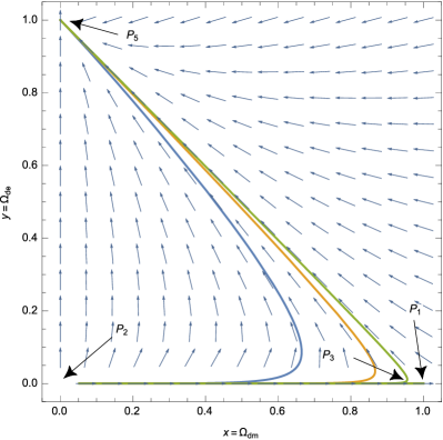
Figure 1 shows projections of some example orbits in the plane (, ) to illustrate the above scenario.
4 Concluding remarks
In this work, we studied the dynamics of a model of the Universe filled with radiation, dark matter, and dark energy. The dark matter component was treated as an imperfect fluid having bulk viscosity in the framework of a Maxwell-Cattaneo approach. Whereas the remaining fluids were considered as perfect fluids. The bulk viscosity was taken as proportional to the Hubble parameter Kremer2012 ; AvelinoLeyvaUrena-Lopez2013 ; Acquaviva2014 .
In order to investigate the asymptotic evolution of the model, we performed a dynamical system analysis. This analysis was based on the requirement of a transition from a RDE to a MDE, at early and intermediate stages, to finally converge to an accelerated solution at late times. This statement, together with a recent estimation of the dark matter EOS reduce the bulk viscosity parameter to a very small region, namely . This result reproduces similar results obtained in the non-causal Eckart framework in VeltenSchwarz2012 ; VeltenSchwarzFabrisEtAl2013 ; CruzLepeLeyvaEtAl2014 ; Leyva2017 and more recently by Lepe2017 in the IsraelStewart formalism.
In the absence of a dark energy fluid, the model is able to reproduce a stable accelerated solution in the quintessence region due to the contribution of the bulk viscosity pressure. However, this solution is ruled out as a possible answer to the present period of accelerated expansion of the Universe since it is impossible to reproduce previous periods of radiation and dark matter domination.
From the stability point of view, the late time attractor, compatible with previous stages of radiation and matter dominations, is always an accelerated solution. This can be a phantom() or quintessence () solutions. The nature of both possible solutions depends only on the barotropix index of the dark energy fluid, namely . Hence, the only way this model is able to cross the phantom divide () is taking a phantom fluid () as a dark energy source. Thus the possible transitions are: (RDE) (MDE) or (RDE) (MDE).
In all the cases, the source of any orbits in the phase space is the stiff matter solution 999This critical point is equivalent to in Lepe2017 , where the IsraelStewart formalism is used for a different parametrization of the bulk viscosity.. Contrary to the late time case, this point exhibit a contribution of a positive bulk viscosity pressure. This explains the extremely high values taken by the variable, and consequently by the bulk viscosity pressure , at this period of the evolution of the Universe in this model.
References
- (1) Edmund J. Copeland, M. Sami, and Shinji Tsujikawa. Dynamics of dark energy. Int. J. Mod. Phys., D15:1753–1936, 2006.
- (2) Shin’ichi Nojiri and Sergei D. Odintsov. Introduction to modified gravity and gravitational alternative for dark energy. eConf, C0602061:06, 2006. [Int. J. Geom. Meth. Mod. Phys.4,115(2007)].
- (3) Timothy Clifton, Pedro G. Ferreira, Antonio Padilla, and Constantinos Skordis. Modified Gravity and Cosmology. Phys. Rept., 513:1–189, 2012.
- (4) Kazuharu Bamba, Salvatore Capozziello, Shin’ichi Nojiri, and Sergei D. Odintsov. Dark energy cosmology: the equivalent description via different theoretical models and cosmography tests. Astrophys. Space Sci., 342:155–228, 2012.
- (5) Luca Amendola and Shinji Tsujikawa. Dark Energy. Cambridge University Press, 2015.
- (6) Kazuya Koyama. Cosmological Tests of Modified Gravity. Rept. Prog. Phys., 79(4):046902, 2016.
- (7) P. A. R. Ade et al. Planck 2015 results. XIII. Cosmological parameters. Astron. Astrophys., 594:A13, 2016.
- (8) S. Weinberg. The cosmological constant problem. Reviews of Modern Physics, 61:1–23, January 1989.
- (9) Antonio Padilla. Lectures on the Cosmological Constant Problem. 2015.
- (10) T. Padmanabhan and Hamsa Padmanabhan. CosMIn: The Solution to the Cosmological Constant Problem. Int. J. Mod. Phys., D22:1342001, 2013.
- (11) Shin’ichi Nojiri. Some solutions for one of the cosmological constant problems. Mod. Phys. Lett., A31(37):1650213, 2016.
- (12) Iver H. Brevik and L. T. Heen. Remarks on the viscosity concept in the early universe. Astrophys. Space Sci., 219:99, 1994.
- (13) Winfried Zimdahl. ’Understanding’ cosmological bulk viscosity. Mon. Not. Roy. Astron. Soc., 280:1239, 1996.
- (14) Shin’ichi Nojiri and Sergei D. Odintsov. Quantum de Sitter cosmology and phantom matter. Phys. Lett., B562:147–152, 2003.
- (15) Shin’ichi Nojiri and Sergei D. Odintsov. Inhomogeneous equation of state of the universe: Phantom era, future singularity and crossing the phantom barrier. Phys. Rev., D72:023003, 2005.
- (16) Shin’ichi Nojiri and Sergei D. Odintsov. Unifying phantom inflation with late-time acceleration: Scalar phantom-non-phantom transition model and generalized holographic dark energy. Gen. Rel. Grav., 38:1285–1304, 2006.
- (17) Vincenzo F. Cardone, C. Tortora, A. Troisi, and S. Capozziello. Beyond the perfect fluid hypothesis for dark energy equation of state. Phys. Rev., D73:043508, 2006.
- (18) I. Brevik, E. Elizalde, S. Nojiri, and S. D. Odintsov. Viscous Little Rip Cosmology. Phys. Rev., D84:103508, 2011.
- (19) I. Brevik, R. Myrzakulov, S. Nojiri, and S. D. Odintsov. Turbulence and Little Rip Cosmology. Phys. Rev., D86:063007, 2012.
- (20) Nouraddin Mostafapoor and Oyvind Gron. Bianchi Type-I Universe Models with Nonlinear Viscosity. Astrophys. Space Sci., 343:423–434, 2013.
- (21) Iver Brevik. Viscosity-Induced Crossing of the Phantom Barrier. Entropy, 17:6318–6328, 2015.
- (22) I. Brevik, V. V. Obukhov, and A. V. Timoshkin. Dark Energy Coupled with Dark Matter in Viscous Fluid Cosmology. Astrophys. Space Sci., 355:399–403, 2015.
- (23) Kazuharu Bamba and Sergei D. Odintsov. Inflation in a viscous fluid model. Eur. Phys. J., C76(1):18, 2016.
- (24) Athira Sasidharan and Titus K. Mathew. Phase space analysis of bulk viscous matter dominated universe. JHEP, 06:138, 2016.
- (25) Carlos E. Laciana. A causal viscous cosmology without singularities. Gen. Rel. Grav., 49(5):62, 2017.
- (26) O. Gron. Viscous inflationary universe models. Astrophys. Space Sci., 173:191–225, 1990.
- (27) Roy Maartens. Dissipative cosmology. Class. Quant. Grav., 12:1455–1465, 1995.
- (28) Iver Brevik and Øyvind Grøn. Relativistic Viscous Universe Models. In Anderson Travena and Brady Soren, editors, Recent Advances in Cosmology, pages 97–127. 2014.
- (29) Iver Brevik, Øyvind Grøn, Jaume de Haro, Sergei D. Odintsov, and Emmanuel N. Saridakis. Viscous Cosmology for Early- and Late-Time Universe. Int. J. Mod. Phys., D26:1730024, 2017.
- (30) Carl Eckart. The Thermodynamics of irreversible processes. 3.. Relativistic theory of the simple fluid. Phys. Rev., 58:919–924, 1940.
- (31) Baojiu Li and John D. Barrow. Does Bulk Viscosity Create a Viable Unified Dark Matter Model? Phys. Rev., D79:103521, 2009.
- (32) Arturo Avelino and Ulises Nucamendi. Can a matter-dominated model with constant bulk viscosity drive the accelerated expansion of the universe? JCAP, 0904:006, 2009.
- (33) Hermano Velten and Dominik J. Schwarz. Constraints on dissipative unified dark matter. JCAP, 1109:016, 2011.
- (34) Hermano Velten and Dominik Schwarz. Dissipation of dark matter. Phys. Rev., D86:083501, 2012.
- (35) H. Velten, D. J. Schwarz, J. C. Fabris, and W. Zimdahl. Viscous dark matter growth in (neo-)Newtonian cosmology. Phys. Rev., D88(10):103522, 2013.
- (36) Hermano Velten, Jiaxin Wang, and Xinhe Meng. Phantom dark energy as an effect of bulk viscosity. Phys. Rev., D88:123504, 2013.
- (37) Arturo Avelino, Yoelsy Leyva, and L. Arturo Urena-Lopez. Interacting viscous dark fluids. Phys. Rev., D88:123004, 2013.
- (38) Norman Cruz, Samuel Lepe, Yoelsy Leyva, Francisco Peña, and Joel Saavedra. No stable dissipative phantom scenario in the framework of a complete cosmological dynamics. Phys. Rev., D90(8):083524, 2014.
- (39) Yoelsy Leyva and Mirko Sepúlveda. Bulk viscosity, interaction and the viability of phantom solutions. Eur. Phys. J., C77(6):426, 2017.
- (40) W. Israel and J. M. Stewart. Transient relativistic thermodynamics and kinetic theory. Annals Phys., 118:341–372, 1979.
- (41) Roy Maartens. Causal thermodynamics in relativity. 1996.
- (42) Mohamed Zakari and David Jou. Equations of state and transport equations in viscous cosmological models. Phys. Rev., D48(4):1597, 1993.
- (43) H. P. de Oliveira and J. M. Salim. Nonequilibrium Friedmann Cosmologies. Acta Phys. Polon., B19:649, 1988.
- (44) D. Pavon, J. Bafaluy, and D. Jou. Causal Friedmann-Robertson-Walker cosmology. Class. Quant. Grav., 8:347–360, 1991.
- (45) Norman Cruz, Samuel Lepe, and Francisco Peña. Crossing the phantom divide with dissipative normal matter in the Israel–Stewart formalism. Phys. Lett., B767:103–109, 2017.
- (46) S. Chapman and T. G. Cowling. The Mathematical Theory of Non-uniform Gases. January 1991.
- (47) W. A. Hiscock and J. Salmonson. Dissipative Boltzmann-Robertson-Walker cosmologies. Phys. Rev., D43:3249–3258, 1991.
- (48) Sangyong Jeon. Hydrodynamic transport coefficients in relativistic scalar field theory. Phys. Rev., D52:3591–3642, 1995.
- (49) Sangyong Jeon and Laurence G. Yaffe. From quantum field theory to hydrodynamics: Transport coefficients and effective kinetic theory. Phys. Rev., D53:5799–5809, 1996.
- (50) Mar Bastero-Gil, Arjun Berera, Rafael Cerezo, Rudnei O. Ramos, and Gustavo S. Vicente. Stability analysis for the background equations for inflation with dissipation and in a viscous radiation bath. JCAP, 1211:042, 2012.
- (51) Jie Ren and Xin-He Meng. Cosmological model with viscosity media (dark fluid) described by an effective equation of state. Phys. Lett., B633:1–8, 2006.
- (52) Ming-Guang Hu and Xin-He Meng. Bulk viscous cosmology: statefinder and entropy. Phys. Lett., B635:186–194, 2006.
- (53) Gilberto M. Kremer and Octavio A. S. Sobreiro. Bulk viscous cosmological model with interacting dark fluids. Braz. J. Phys., 42:77–83, 2012.
- (54) G. Acquaviva and A. Beesham. Nonlinear bulk viscosity and the stability of accelerated expansion in FRW spacetime. Phys. Rev., D90(2):023503, 2014.
- (55) Jaume Haro and Supriya Pan. Bulk viscous quintessential inflation. 2015.
- (56) Deng Wang, Yang-Jie Yan, and Xin-He Meng. Constraining viscous dark energy models with the latest cosmological data. Eur. Phys. J., C77(10):660, 2017.
- (57) Roy Maartens and Vicenc Mendez. Nonlinear bulk viscosity and inflation. Phys. Rev., D55:1937–1942, 1997.
- (58) Genly Leon, Yoelsy Leyva, and J. Socorro. Quintom phase-space: beyond the exponential potential. Phys. Lett., B732:285–297, 2014.
- (59) Winfried Zimdahl and Diego Pavon. Expanding universe with positive bulk viscous pressures? Phys. Rev., D61:108301, 2000.
- (60) Charles W. Misner, K. S. Thorne, and J. A. Wheeler. Gravitation. W. H. Freeman, San Francisco, 1973.
- (61) Daniel B. Thomas, Michael Kopp, and Constantinos Skordis. Constraining dark matter properties with Cosmic Microwave Background observations. Astrophys. J., 830(2):155, 2016.
- (62) Samuel Lepe, Giovanni Otalora, and Joel Saavedra. Dynamics of viscous cosmologies in the full Israel-Stewart formalism. Phys. Rev., D96(2):023536, 2017.