Spatial Channel Covariance Estimation
for the Hybrid MIMO Architecture:
A Compressive Sensing Based Approach
Abstract
Spatial channel covariance information can replace full knowledge of the entire channel matrix for designing analog precoders in hybrid multiple-input-multiple-output (MIMO) architecture. Spatial channel covariance estimation, however, is challenging for the hybrid MIMO architecture because the estimator operating at baseband can only obtain a lower dimensional pre-combined signal through fewer radio frequency (RF) chains than antennas. In this paper, we propose two approaches for covariance estimation based on compressive sensing techniques. One is to apply a time-varying sensing matrix, and the other is to exploit the prior knowledge that the covariance matrix is Hermitian. We present the rationale of the two ideas and validate the superiority of the proposed methods by theoretical analysis and numerical simulations. We conclude the paper by extending the proposed algorithms from narrowband massive MIMO systems with a single receive antenna to wideband systems with multiple receive antennas.
I Introduction
One way to increase coverage and capacity in wireless communication systems is to use a large number of antennas. For instance, millimeter wave systems use large antenna arrays to obtain high array gain, thereby increasing cellular coverage [1, 2]. Sub-6 GHz systems are also likely to equip many antennas at a base station (BS) to increase cellular spectral efficiency by transmitting data to many users simultaneously via massive MIMO systems [3, 4]. Using a large number of antennas in a conventional MIMO architecture, however, results in high cost and high power consumption because each antenna requires its own RF chain [5]. To solve this problem, hybrid analog/digital precoding reduces the number of RF chains by dividing the linear process between the analog RF part and the digital baseband part. Several hybrid precoding techniques have been proposed for single-user MIMO [6, 7, 8, 9] and multi-user MIMO [10, 11, 12, 13, 14] in either sub-6 GHz systems or millimeter wave systems.
Most prior work on hybrid precoding assumes that full channel state information at the transmitter (CSIT) for all antennas is available when designing the analog precoder. Full CSIT, however, is difficult to obtain even in time-division duplexing (TDD) systems if many antennas are employed. Furthermore, the hybrid structure makes it more difficult to estimate the full CSIT of the entire channel matrix for all antennas because the estimator can only see a lower dimensional representation of the entire channel due to the reduced number of RF chains. Although some channel estimation techniques for the hybrid architecture were proposed by using compressive sensing techniques that exploit spatial channel sparsity [15, 16, 17], these techniques assume that channel does not change during the estimation process which requires many measurements over time. Consequently, these channel estimation techniques can be applied only to slowly varying channels.
Unlike the hybrid precoding techniques that require full CSIT, there exists another type of hybrid precoding that uses long-term channel statistics such as spatial channel covariance instead of full CSIT in the analog precoder design [13, 14, 18, 19]. This approach has advantages over using full CSIT. First, the spatial channel covariance is well modeled as constant over many channel coherence intervals [20, 18]. Second, the spatial channel covariance is constant over frequency in general [21], so covariance information is suitable for the wideband hybrid precoder design problem where one common analog precoder must be shared by all subcarriers in wideband OFDM systems [9]. For these reasons, spatial channel covariance information is a promising alternative to full CSIT for hybrid MIMO architecture.
Although several techniques have been developed to estimate spatial channel covariance or its simplified version such as subspace or angle-of-arrival (AoA) for hybrid architecture, these methods have practical issues. For example, the sparse array developed in [22] and the coprime sampling used in [23] reduce the number of RF chains for the covariance or AoA estimation as they disregard some of the antennas by exploiting redundancy in linear arrays of equidistant antennas. These methods, however, have a limitation on the configuration of the number of RF chains and antennas. In [24], various estimation methods were proposed based on convex optimization problems coupled with the coprime sampling. The proposed methods, though, require many iterations to converge. A subspace estimation method using the Arnoldi iteration was proposed for millimeter wave systems in [25]. The estimation target of this method is not the subspace of a spatial channel covariance matrix but that of a channel matrix itself, and the channel matrix must be constant over time during the estimation process. Consequently, it is difficult to apply the method in [25] to time-varying channels. The subspace estimation method proposed in [26] does not use any symmetry properties of the covariance matrix, while the AoA estimation for the hybrid structure in [27] does not exploit the sparse property of millimeter wave channels. In [28, 29], AoA estimation methods for the hybrid structure were proposed by applying compressive sensing techniques with vectorization but do not fully exploit the slow varying AoA property. Instead of using a vector-type compressive sensing, matrix-type compressive sensing techniques were developed for so-called multiple measurement vector (MMV) problems [30, 31, 32, 33]. Most prior work on the MMV problems, however, assumes that the sensing matrix is fixed over time to model the problem in a matrix form, which is not an efficient strategy when the measurement size becomes as small as the sparsity level.
In this paper, we propose a novel spatial channel covariance estimation technique for the hybrid MIMO architecture. Considering spatially sparse channels, we develop the estimation technique based on compressive sensing techniques that leverage the channel sparsity. Between two different approaches in the compressive sensing field (convex optimization algorithms vs. greedy algorithms), we focus on the greedy approach because they provide a similar performance to convex optimization algorithms in spite of their simpler complexity [34]. Based on well-known greedy algorithms such as orthogonal matching pursuit (OMP) and simultaneous OMP (SOMP), we improve performance by applying two key ideas: one is to use a time-varying sensing matrix, and the other is to exploit the fact that covariance matrices are Hermitian. Motivated by the fact that SOMP is a generalized version of OMP, we develop a further generalized version of SOMP by incorporating the proposed ideas. The algorithm modification is simple, but the performance improvement is significant, which is demonstrated by numerical and analytical results.
We first develop the spatial channel covariance estimation work for a simple scenario where a mobile station (MS) has a single antenna in narrowband systems. Preliminary results were presented in the conference version of this paper [35]. In this paper, we add two new contributions to our prior work. First, we present theoretical analysis to validate the rationale of the two proposed ideas and show the superiority of the proposed algorithm. The theoretical analysis demonstrates that the use of a time-varying sensing matrix dramatically improves the covariance estimation performance, in particular, when the number of RF chains is not so large and similar to the number of channel paths. The analytical results also disclose that exploiting the Hermitian property of the covariance matrix provides an additional gain. Second, we extend the estimation work to other scenarios. Considering that an MS as well as a BS has hybrid architecture with multiple antennas and RF chains, we modify the proposed algorithm to adapt to the situation where analog precoders as well as analog combiners change over time. We also modify the algorithm for the wideband systems by using the fact that frequency selective baseband combiners do not improve the estimation performance.
We use the following notation throughout this paper: is a matrix, is a vector, is a scalar, and is a set. and are the -norm and -norm of a vector . denotes a Frobenius norm. , , , and are transpose, conjugate, conjugate transpose, and Moore-Penrose pseudoinverse. and are the -th row and -th column of the matrix . denotes a matrix whose columns are composed of for . If there is nothing ambiguous in the context, , , , and are replaced by , , , and . is the relative complement of in , is a column vector whose elements are the diagonal elements of , and is the cardinality of . , , and denote the Kronecker product, the Hadamard product, and the column-wise Khatri-Rao product. is the generalized Khatri-Rao product with respect to partitions, which is defined as where and .
II System model and preliminaires: covariance estimation via compressive sensing based channel estimation
In this section, we present the system model and briefly overview prior work on compressive sensing based channel estimation followed by covariance calculation.
II-A System model
Consider a system where a BS with antennas and RF chains communicates with an MS. We focus on a narrowband massive MIMO system where an MS with a single antenna; we extend the work to the multiple-MS-antenna case and the wideband case in Section V. Let be the number of channel paths, be a time-varying channel coefficient of the -th channel path at the -th snapshot, and be an array response vector associated with the AoA of the -th channel path . Assuming that AoAs do not change during snapshots, the uplink channel at the -th snapshot can be represented as
| (1) |
Considering spatially sparse channels, the channel model in (1) can be approximated in the compressive sensing framework as
| (2) |
where is an dictionary matrix whose columns are composed of the array response vectors associated with a predefined set of AoAs, and is a sparse vector with only nonzero elements whose positions and values correspond to their AoAs and path gains.
Let be a training symbol with , and be a Gaussian noise with . The received signal can be represented as
| (3) |
Combined with an analog combining matrix , the received signal multiplied by at baseband is expressed as
| (4) |
where denotes an overall sensing matrix and . By letting , the spatial channel covariance matrix is expressed as . The goal is to estimate with given .
II-B Preliminaires: covariance estimation via compressive sensing based channel estimation
Some prior work developed compressive channel estimators for the hybrid architecture [15, 16, 17]. Once the channel vectors are estimated, the covariance can be calculated from the estimated channels. In this section, we overview two estimation approaches to make a comparison.
A baseline technique to estimate the channel vector at each time is formulated as
| (5) |
This optimization problem is known as a single measurement vector (SMV) problem and can be solved by the OMP algorithm described in Algorithm 1, which is a simple but efficient approach among various solutions to the SMV problem [36]. Once the ’s are estimated during snapshots, then the covariance matrix of the channel can be calculated as
| (6) |
In contrast to SMV, another compressive sensing technique called MMV [30] exploits the observation that shares a common support if the AoAs do not change during the estimation process. The received signal model in (4) can be written in a matrix form as
| (7) |
where , , and . Note that in this MMV problem format, the sensing matrix must be common over time. The optimization problem in the MMV is formulated as
| (8) |
where represents the row sparsity defined as . This optimization problem can be solved by the SOMP algorithm described in Algorithm 2 [37, 38]. Regarding the selection rule of SOMP, the -norm in Algorithm 2 can be replaced by the -norm because there is no significant difference between the two in terms of performance [31]. We use -norm throughout this paper for analytical tractability. Although SOMP is known to outperform OMP in general, SOMP still needs improvement, particularly when the number of RF chains is small, as will be discussed in Section III-A.
III Covariance estimation for hybrid architecture: two key ideas
In this section, we present two key ideas to improve covariance estimation work based on compressive sensing techniques. First, we develop an estimation algorithm by applying a time-varying sensing matrix. Second, we propose another algorithm that exploits the Hermitian property of the covariance matrix. Finally, we combine the two proposed algorithms.
III-A Applying a time-varying analog combining matrix
Although compressive sensing can reduce the required number of measurements, there is a limitation on reducing the measurement size. This lower bound is known to be for both SMV and MMV when the sensing matrix satisfies the restricted isometry property (RIP) condition. [39]. One possible solution to overcome this limitation is to extend the measurement vector size into the time domain, i.e., gathering the measurement vectors of multiple snapshots with different sensing matrices over time. The same approach is also used in [15] and [36], where the measurements are stacked together as
| (9) |
Note that the key assumption in (9) is that is constant during the estimation process. Consequently, this technique can be applied only to static channels, not time-varying channels.
It is worthwhile to compare the MMV signal model in (7) with the signal model where the time-varying combining matrix is used for the static channel as shown in (9). In (7), ’s are stacked in columns due to the fact that changes over time but is fixed. In contrast, the signal model in (9) adopts a row-wise stack of because changes over time but is fixed. If both and change over time, we can not stack ’s in either columns or rows and thus need another approach. Regarding this scenario, two questions arise: 1) is it useful to employ a time-varying sensing matrix for a time-varying channel? 2) how can we recover the data in this time-varying sensing matrix and time-varying data? We will show that the time-varying sensing matrix can increase the recovery success rate especially when is not much larger than by analysis in Section IV and simulations in Section VI. In this subsection, we develop a recovery algorithm to answer the problem of recovery with a time-varying sensing matrix.
To apply the time-varying matrix concept to SOMP, we first focus on the fact that SOMP is a generalized version of OMP. The reason is that the optimization problem of MMV in (8) can be rewritten as
| (10) |
Note that SOMP is equivalent to OMP when . Unlike the original formulation in (8), this reformulated form gives an insight into how to apply the time-varying sensing matrix. We can further generalize the optimization problem in (10) by replacing with to reflect the time-varying feature of the sensing matrix. Noting that the selection rule of SOMP in Algorithm 2 is equivalent to , we modify the selection rule by replacing with to adapt to the time-varying sensing matrix case. The residual matrix in SOMP, , can also be replaced by for . The modified version of SOMP, which we call dynamic SOMP (DSOMP), is described in Algorithm 3.
III-B Exploiting the Hermitian property of the covariance matrix
The covariance estimation techniques using OMP, SOMP, and DSOMP in the previous subsections employ a two-step approach where the channel gain vectors ’s (and thus channel vectors ’s) are estimated and then the covariance matrix is calculated from (6). If it is not the channel but the covariance that needs to be estimated, the first step estimating the channel explicitly is unnecessary. In this subsection, we take a different approach that directly estimates the covariance without estimating the instantaneous channel gain vectors.
The relationship between and is given by
| (11) |
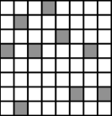
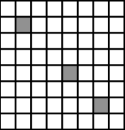
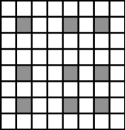
If we consider a special case where is assumed to be a sparse diagonal matrix as in Fig. 1(c), the relationship between and in (11) can be rewritten as
| (12) |
by using vectorization and the column-wise Khatri-Rao product, then OMP can be directly applied to this reformulated problem without any modification [40]. This approach, however, has a limitation in application to realistic scenarios because the covariance is not a diagonal matrix in general [35]. Instead of assuming that is a sparse diagonal matrix, we consider to be a sparse Hermitian matrix as in Fig. 1(d). As MMV uses the fact that is a matrix with sparse rows as in Fig. 1(b), we exploits the Hermitian property of the covariance matrix . The optimization problem is represented in a matrix form like MMV,
| (13) |
where is defined as .

A greedy approach similar to OMP and SOMP can be applied to find a suboptimal solution. At each iteration, the algorithm needs to find the solution to the following sub-problems as
| (14) |
where is a Hermitian matrix whose dimension is less than or equal to . By using the least squares method along with vectorization, the optimal solution to (14) is given by
| (15) |
where . Note that if is Hermitian, is also Hermitian. The proposed algorithm using (15), which we call covariance OMP (COMP), is described in Algorithm 4. Note that the proposed COMP uses quadratic forms instead of linear forms.
The time-varying sensing matrix concept in Section III-A can also be applied to COMP. The generalization of COMP, however, requires a careful modification. In covariance estimation based on COMP, the calculation of is followed by the estimation of . This is because can be represented as a function of as
| (16) |
If the sensing matrix changes over time, can not be represented as a function of because
| (17) |
For this reason, instead of using the sample covariance matrix of the measurement vectors , we use a per-snapshot , which can be regarded as a one sample estimate of the sample covariance matrix. Note that this extreme sample covariance is not a diagonal matrix in general even when the channel paths are uncorrelated. Using the fact that for all snapshots are sparse Hermitian matrices sharing the same positions of nonzero elements, we develop the dynamic COMP (DCOMP) from COMP in a similar way that we develop DSOMP from SOMP, which is described in Algorithm 5. Note that DCOMP becomes equivalent to COMP if .
IV Theoretical analysis of the proposed alogirhtms
In this section, we analyze the benefit of the time-varying sensing matrix and compare SOMP, DSOMP, and DCOMP. In summary, the recovery success probability of SOMP, DSOMP, and DCOMP increases as the number of measurements increases. The recovery success probability of SOMP, however, saturates and does not approach one as goes to infinity even in the noiseless case if the number of RF chains is not much larger than the number of channel paths . In contrast to SOMP, the recovery success probability of DSOMP and DCOMP approaches one as increases for any and . In other words, DSOMP and DCOMP can guarantee perfect recovery even when the number of RF chains is so small that both OMP and SOMP fail to recover the support even in the noiseless case. Finally, we will show that DCOMP has a higher recovery success probability than DSOMP.
Let us first consider how to design the sensing matrix . For analytical tractability, we confine the dictionary size to in this section. The algorithms, however, can be applied to more general cases such as . The sensing matrix can be represented as . One possible option for the sensing matrix is to use a random analog precoding matrix such that each element in has a constant amplitude and a random phase with an independent uniform distribution in [0, ]. Since the elements in the sensing matrix designed in this way have a sub-Gaussian distribution, this simple random sensing matrix satisfies the RIP condition [34]. There are other desirable features that the sensing matrix needs to have. For example, it is desirable for the sensing matrix to have a small mutual coherence defined as [34]. The mutual coherence has a lower bound , which is known as Welch bound. This bound can be achievable if the column vectors in constitute an equal-norm equiangular tight frame, i.e., satisfies that 1) , 2) , and 3) . It is impossible for a sensing matrix that is designed with a random phase analog combining matrix to meet these three conditions at all times. Nevertheless, it is possible to meet the tight frame condition for any random analog precoding matrix if the baseband combining matrix is employed such that
| (18) |
If the baseband combining matrix is designed as (18), the columns in the overall sensing matrix constitute the tight frame because it satisfies
| (19) |
Consequently, any sensing matrix can be transformed to satisfy the tight frame condition by using .
The following theorem provides the exact condition for the perfect recovery condition at each iteration of the DSOMP algorithm. Note that OMP and SOMP are special cases of DSOMP.
Theorem 1
Let be an optimal support set with and be an ideal channel gain matrix. Suppose that with was perfectly recovered at the previous iterations in the DSOMP algorithm. In the noiseless case, one of the elements in the optimal support can be perfectly recovered at the -th iteration if and only if
| (20) |
where .
Proof:
See Appendix A. ∎
Although the newly defined metric identifies the exact condition for the perfect recovery condition, its dependence on the input data makes this metric less attractive. Some prior work takes an approach to find upper bounds of certain coherence-related metrics for any random input data [41], but the bounds are loose, which can be regarded as a worst case analysis. In addition, those upper bounds are meaningful only for the case where is significantly larger than . In the extreme case where and are similar in value, the upper bounds are too loose to give a useful insight.
Instead of an upper bound, we focus on the distribution of considering , , , and as random variables. While the exact distribution depends on the distribution of , Proposition 1 and Theorem 2 show that converges to a value that does not depend on as becomes larger.
Proposition 1
Suppose that are independent random variables with zero mean and unit variance. Let denote in the SOMP case where . As , converges to
| (21) |
where .
Proof:
See Appendix B. ∎
Note that in (21) can be rewritten as
| (22) |
In the OMP case, becomes equivalent to
| (23) |
where . Since the addition of a random variable results in increasing the variance of the metric at , the maximum values in both the numerator and the denominator for the OMP case are likely to be larger than those of the SOMP case. Compared with the SOMP case, the relative rate of increase in the numerator is higher than that of increase in the denominator with high possibility because is larger than for in general for a random sensing matrix. Consequently, we can infer that the normalized coherence metric of SOMP is likely to be less than that of OMP. We validate this inference by simulations for random , , and in Section VI-A.
Although this explains the superiority of SOMP over OMP, we can see that the probability of does not become one in general. This means that SOMP can not guarantee the perfect recovery even when an infinite number of snapshots are measured for the recovery.
Unlike SOMP, DSOMP can always guarantee perfect recovery as becomes larger as shown in the following theorem.
Theorem 2
As , in (20) converges to a deterministic value that has an upper bound as
| (24) |
and this upper bound is always less than or equal to one for any , i.e,. perfect recovery is guaranteed.
Proof:
See Appendix C. ∎
In Section VI, we show by simulations that a reasonably small can provide a significant gain over SOMP even in the extreme case when . In addition, the converged value of DSOMP is not a function of sensing matrices while that of SOMP depends on the sensing matrix . In other words, in contrast to the SOMP case where sophisticated sensing matrix design is crucial to the estimation performance, DSOMP can reduce the necessity of the elaborate design of the sensing matrix as increases.
Similar to the DSOMP case, DCOMP can also guarantee the perfect recovery. The perfect recovery condition of the DCOMP case is shown in the following theorem.
Theorem 3
Let be an optimal support set with and be an ideal channel gain matrix. Suppose that with was perfectly recovered at the previous iterations in the DCOMP algorithm. In the noiseless case, one of the elements in the optimal support can be perfectly recovered at the -th iteration if and only if
| (25) |
where and .
Proof:
From the definition of the residual matrix in Algorithm 5, the selection rule of DCOMP can be represented as
| (26) |
and this completes the proof. ∎
Let . Notice that, if is replaced by , then Theorem 3 becomes identical to Theorem 1. It is also worthwhile to note that both DSOMP and DCOMP select the same support at the first iteration because for . The superiority of DCOMP over DSOMP starts from the second iteration, which can be inferred from the following theorem.
Theorem 4
in (25) converges to a deterministic value as , and the deterministic value always satisfies
| (27) |
for any .
Proof:
See Appendix D. ∎
Until now, we considered a time-varying analog combining matrix and its associated digital combining matrix. One question arises: if the analog combiner is fixed and only the digital combiner is time-varying, does the time variance of the baseband combiner improve the recovery performance? The following proposition shows that the time-varying baseband combining matrix itself does not improve the performance when the analog combining matrix is fixed.
Proposition 2
Let for a fixed and a random unitary matrix such that constitutes a tight frame for any . Then, of DSOMP becomes identical to of SOMP where .
Proof:
Each term in both the numerator and the denominator in (51) becomes
| (28) |
because and for all . Since this is the same as in the SOMP case where , the proof is completed. ∎
The result in Proposition 2 is beneficial especially to the wideband case where the analog combining matrix must be fixed over frequency. According to Proposition 2, we will use the frequency-invariant baseband combining matrix when modifying the algorithm for the wideband case. This will be discussed in more detail in Section V-B.
V Extension to other scenarios
In Section III, we considered a narrowband system and assumed that an MS has a single antenna. In this section, we first extend the work to the multiple-MS-antenna case and then to the wideband case.
V-A Extension to the multiple-MS-antenna case
In this subsection, we extend the work in Section III to the case where the MS has hybrid architecture with multiple antennas and RF chains. The signal model is shown in Fig. 2 where , , , and denote the number of transmit antennas, transmit RF chains, receive antennas, and receive RF chains. We assume that consecutive training symbols are used in each frame as shown in Fig. 2, and the symbol index per frame is denoted by . We assume that the duration of symbols is less than the channel coherence time, i.e., the channel is invariant during consecutive symbol transmission. Let be the angle of departure (AoD) of the -th path. The channel model for the single-MS-antenna case in (1) can be extended to the multiple-MS-antenna case as
| (29) |
Similarly to (2), this can also be represented in the compressive sensing framework as , where and are dictionary matrices associated with AoA and AoA, and is a sparse matrix with nonzero elements with associated with complex channel path gains.
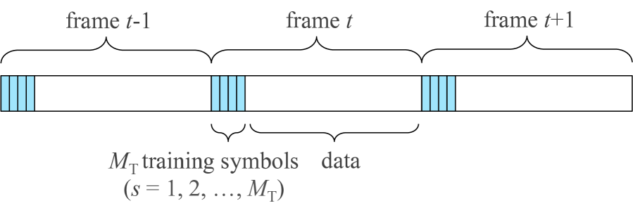
At each symbol at frame , one training signal is transmitted through one transmit RF chain. Let be a combiner and a precoder at frame and symbol . Assuming that the training symbol is known to the BS, thereby omitted as in the single-MS-antenna case, the received signal at baseband is represented as
| (30) |
There are four different types with respect to how to apply and within a frame: 1) fixed and fixed , 2) time-varying and fixed , 3) fixed and time-varying , and 4) time-varying and time-varying .
In the first approach, all the precoders are the same within a frame, and so are the combiners such that and . Since these combiners and precoders are constant within a frame in this approach, averaging the received signals at baseband within a frame can increase the effective signal-to-noise ratio (SNR). The averaged received signal is represented as
| (31) |
where . Note that , which means that this process averages out the noise, increasing the effective SNR. The signal model per frame in (31) can be transformed into
| (32) |
In the second approach, where only combiners vary and precoders are fixed within a frame such that , the first step is to stack in rows. This row-wise stack yields a vector per frame,
| (33) |
where and . The signal model in (33) can be rewritten as
| (34) |
The third approach changes only precoders, and combiners are fixed within a frame such that . In contrast to the second approach, are stacked in columns. This column-wise stack makes the aggregate signal model per frame as
| (35) |
where , , and . By using vectorization, the matrix in (35) can be transformed into a vector form as
| (36) |
For the last approach, both precoders and combiners change within a frame. Like the second approach, we stack in rows. Then, the row-wise stacked vector becomes
| (37) |
Note that the signal models for all four different approaches in (32), (34), (36), and (37) can be generalized as where , , and are dependent on each approach. This generalized signal model has the same format as that of the single-MS-antenna case in (4). Consequently, the algorithm proposed for the single-MS-antenna case such as DCOMP can be used without any modification in the multiple-MS-antenna case regardless of different approaches.
V-B Extension to wideband systems
In this subsection, we extend our work in the narrowband case into the wideband case. Since the same algorithm can be used for both the single-MS-antenna case and the multiple-MS-antenna case as shown in Section V-A, we focus on the single antenna case for the sake of exposition.
Compared to the narrowband channel model in (1), we adopt the delay- MIMO channel model for the wideband OFDM systems with subcarriers [42, 43]. Let be the sampling period, be the delay of the -th path, be the cyclic prefix length, and denote a filter comprising the combined effects of pulse shaping and other analog filtering. The delay- MIMO channel matrix is modeled as
| (38) |
and the channel frequency response matrix at each subcarrier can be expressed as
| (39) |
where . This can be cast in the compressive sensing framework as , where and are sparse vectors with nonzero elements associated with and . Note that and share the same support for all and .
An analog combiner at frame must be common for all subcarrier . Since Proposition 2 shows that changing baseband combiners does not impact the performance as long as the analog combiner is fixed, we use a common sensing matrix for all subcarriers at frame . Then, the signal part of the received signal in the baseband at frame and subcarrier is given by .
The problem of finding is similar to the narrowband case in Section III because share the same support for all and . Therefore, the DCOMP algorithm in Section III can be directly applied to this problem. This fails, however, to exploit a useful property of sparse wideband channels. At a fixed subcarrier , the time domain average of becomes
| (40) |
Since (40) has a similar form to (17) of the narrowband case, DCOMP can be used for this time domain operation. The frequency domain average of at a fixed frame can be expressed differently from (40) as
| (41) |
which is similar to (16) of the narrowband case. Since COMP is developed based on the signal model in (16), COMP can be used for the frequency domain operation in the wideband case. The different features between the time and frequency domain motivate us to apply different approaches to each domain, i.e., COMP to the frequency domain and DCOMP to the time domain. This combination of two algorithms, which we call WB-DCOMP, is described in Algorithm 6.
It is worthwhile to compare WB-DCOMP to the direct extension of COMP and DCOMP. If the sensing matrix is varying over both time and frequency, the direct extension of DCOMP provides the best performance. However, if is varying only in the time domain and fixed over frequency, WB-DCOMP, which is the combination of DCOMP and COMP, can outperform the direct extension of each algorithm in the wideband case. This is demonstrated in Section VI.
VI Simulation results
In this section, we validate our analysis in Section IV in terms of the recovery success probability in the noiseless case especially when has a similar value to . We also present simulation results to demonstrate the performance of the proposed spatial channel covariance estimation algorithms for hybrid architecture.
VI-A Theoretical anaylsis in the noiseless case
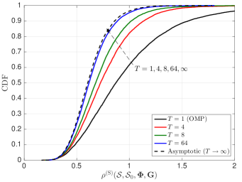
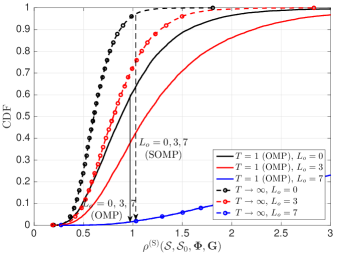
We compare OMP and SOMP in terms of the cumulative distribution function (CDF) of the newly defined metric in (21). Fig. 3 shows how the CDF of changes according to and . In Fig. 3(a), becomes higher as gets larger. In addition, as shown in Proposition 1, the CDF converges to that of in (21) regardless of . Note that indicates the OMP case. Fig. 3(b) shows the CDF versus in the OMP case () and the asymptotic SOMP case (). As increases, the gap between OMP and SOMP reduces and becomes zero if . In this extreme case where , both OMP and SOMP do not work properly because becomes low in the last iteration.
Fig. 4 shows the CDF of in the DSOMP case. Unlike the SOMP case, converges to a deterministic value in (24) for any sensing matrices as increases. The simulation results in Fig. 4 also indicate that has an upper bound as shown in (24), which is consistent with the analytical result in Theorem 2. Although the convergence rate becomes slower as increases, is guaranteed as . Simulation results in Fig. 4 show that a reasonably small value of can ensure a perfect recovery.
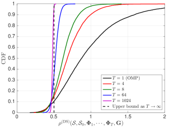
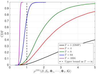
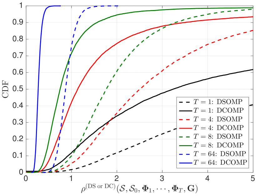
Fig. 5 compares DSOMP and DCOMP. As discussed in Section IV, both select the same support at the first iteration, and the superiority of DCOMP over DSOMP starts from the second iteration. In Fig. 5, the CDF of and are compared in the last iteration, i.e., . The figure shows that the CDF of the DCOMP case is located on the left side of that of the DSOMP case, which means DCOMP has a higher success probability than DSOMP.
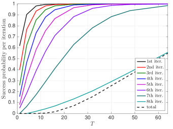
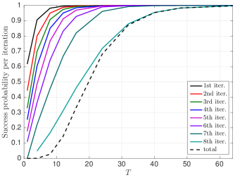
Simulation results with respect to the success probability per iteration is shown in Fig. 6. As expected, the success probability at the first iteration is identical for both DSOMP and DCOMP, but the success probability of DCOMP becomes higher than that of DSOMP from the second iteration, leading to the higher success probability in total.
VI-B Performance evaluation on the covariance estimation for hybrid architecture
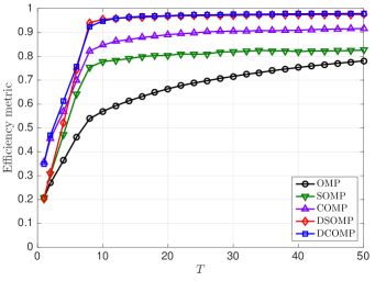
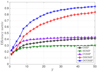
In this subsection, we evaluate the performance of the spatial channel covariance estimation. The performance metric is defined as [24] where and are the matrices whose columns are the eigenvectors of the ideal covariance and the estimated covariance . Note that and a larger indicates a more accurate estimation.
Fig. 7 shows simulation results when , and dB for the single-MS-antenna case in narrowband systems. In the fixed combining matrix case in Fig. 7(a) where , we can see that the proposed COMP outperforms OMP and SOMP. Combined with the time-varying analog combining matrix, DSOMP and DCOMP have more gain over other techniques with a fixed combining matrix. The gap between DSOMP and DCOMP, however, is marginal in this case.
Fig. 7(b) shows the results with 8 RF chains instead of 16 RF chains. As discussed in Section IV, none of the algorithms using a fixed analog combining matrix such as OMP, SOMP, and COMP work properly. Moreover, SOMP even yields worse performance than OMP. In contrast, DSOMP and DCOMP that use a time-varying sensing matrix have a remarkable gain compared to those that use a fixed sensing matrix. In addition, DCOMP, which exploits the Hermitian property of covariance matrices, has a considerable gain compared to DSOMP. These results are consistent with the analysis in Section IV.
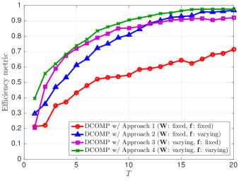
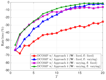
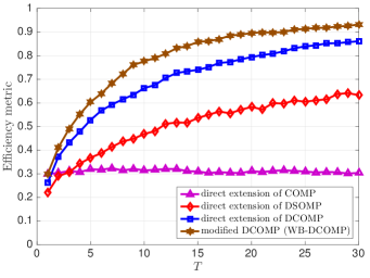
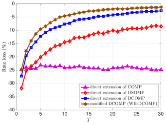
Regarding the extension of the proposed work to the multiple-MS-antenna case, the four different approaches explained in Section V-A are compared in Fig. 8. As expected, the use of time-varying precoding and combining matrices at both BS and MS improves covariance estimation. Fig. 9 shows the extension to the wideband case. As shown in the figure, the combination of COMP and DCOMP outperforms the direct extension of COMP or DCOMP. In addition to the efficiency metric shown in Fig. 8(a) and Fig. 9(a), we evaluate the loss caused by covariance estimation error in terms of spectral efficiency of hybrid precoding. The rate loss in Fig. 8(b) and Fig. 9(b) is defined as in percentage where and are the spectral efficiency of the estimated and ideal covariance case under the assumption that the analog precoding matrix is composed of the dominant eigenvectors of the estimated or ideal spatial channel covariance matrix. The figures show that the trend in the rate loss is consistent with that in the efficiency metric although the rate does not only depend on the efficiency metric but also on other factors such as the type of MIMO techniques and the number of streams.
VII Conclusions
In this paper, we proposed spatial channel covariance estimation techniques for the hybrid MIMO structure. Based on compressive sensing techniques that leverage the spatially sparse property of the channel, we developed covariance estimation algorithms that are featured by two key ideas. One is to apply a time-varying sensing matrix, and the other is to exploit the Hermitian property of the covariance matrix. Simulation results showed that the proposed greedy algorithms outperform prior work, and the benefit of adopting the two ideas becomes more significant as the number of RF chains becomes smaller. We also analyzed the performance of the proposed algorithms in terms of recovery success probability. The theoretical analysis indicated that the success probability approaches one as the number of snapshots increases if a time-varying sensing matrix is applied. The analysis also proved that using the structured property of the covariance matrix improves the estimation performance, which is consistent with the simulation results.
Appendix A Proof of Theorem 1
Let . Then, the support selection criterion at the -th iteration in the DSOMP shown in Algorithm 3 becomes
| (42) |
where comes from and , and comes from due to the characteristics of the orthogonal projection matrix . Consequently, one of the elements in the optimal support is selected, i.e., at iteration if and only if (20) is satisfied.
Appendix B Proof of Proposition 1
If , in (20) becomes
| (43) |
where comes from the fact that are independent random variables with zero mean and unit variance.
Appendix C Proof of Theorem 2
in (20) can be written as
| (44) |
where . In (44), comes from the fact that for all are identical random variables with non-zero mean, for all are identical random variables with zero-mean, and are independent random variables with zero mean and unit variance.
Now let us look at and . Let , then the trace of becomes
| (45) |
where comes from due to the tight frame property, and comes from . From (45), the lower bound of is given by
| (46) |
where comes from the fact that for any random variable .
Now, let us look at the squared Frobenius norm of that is given by
| (47) |
In addition, can be represented differently as
| (48) |
From (46)-(48), the upper bound of can be obtained as
| (49) |
By using the lower bound of and the upper bound of , it can be shown that the converged value of in (44) has an upper bound as
| (50) |
and this upper bound is always less than or equal to one because .
Appendix D Proof of Theorem 4
As , in (20) can be rewritten as
| (51) |
where and comes from the fact that and are independent and all elements in have zero mean and unit variance.
Since the terms in the expectation in (51) and (52) are independent random variables with respect to , we omit the time slot index for simplicity. The difference between the inner parts of the denominators in (51) and (52) becomes
| (53) |
Note that both and can be represented as the production of two semi-unitary matrices, and thus and become positive semidefinite matrices. Since the trace of the product of two semidefinite matrices is larger than or equal to zero, (53) becomes
| (54) |
for any , , and . The difference between the inner parts of the numerators in (51) and (52) becomes
| (55) |
where can be proved by using and .
References
- [1] W. Roh, J. Seol, J. Park, B. Lee, J. Lee, Y. Kim, J. Cho, K. Cheun, and F. Aryanfar, “Millimeter-wave beamforming as an enabling technology for 5G cellular communications: theoretical feasibility and prototype results,” IEEE Comm. Mag., vol. 52, no. 2, pp. 106–113, Feb. 2014.
- [2] R. Heath, N. Gonzlez-Prelcic, S. Rangan, W. Roh, and A. Sayeed, “An overview of signal processing techniques for millimeter wave MIMO systems,” IEEE Jour. Select. Topics in Sig. Proc., vol. 10, no. 3, pp. 436–453, Apr. 2016.
- [3] T. Marzetta, “Noncooperative cellular wireless with unlimited numbers of base station antennas,” IEEE Trans. Wireless Comm., vol. 9, no. 11, pp. 3590–3600, Nov. 2010.
- [4] J. Hoydis, S. ten Brink, and M. Debbah, “Massive MIMO in the UL/DL of cellular networks: How many antennas do we need?” IEEE Jour. Select. Areas in Comm., vol. 31, no. 2, pp. 160–171, Feb. 2013.
- [5] A. F. Molisch, V. V. Ratnam, S. Han, Z. Li, S. L. H. Nguyen, L. Li, and K. Haneda, “Hybrid beamforming for massive MIMO: A survey,” IEEE Comm. Mag., vol. 55, no. 9, pp. 134–141, 2017.
- [6] O. El Ayach, S. Rajagopal, S. Abu-Surra, Z. Pi, and R. Heath, “Spatially sparse precoding in millimeter wave MIMO systems,” IEEE Trans. Wireless Comm., vol. 13, no. 3, pp. 1499–1513, Mar. 2014.
- [7] A. Alkhateeb, O. El Ayach, G. Leus, and R. Heath, “Hybrid precoding for millimeter wave cellular systems with partial channel knowledge,” in Proc. Info. Th. App. (ITA), Feb. 2013, pp. 1–5.
- [8] X. Yu, J. Shen, J. Zhang, and K. Letaief, “Alternating minimization algorithms for hybrid precoding in millimeter wave MIMO systems,” IEEE Jour. Select. Topics in Sig. Proc., vol. 10, no. 3, pp. 485–500, Apr. 2016.
- [9] S. Park, A. Alkhateeb, and R. Heath, “Dynamic subarrays for hybrid precoding in wideband mmWave MIMO systems,” IEEE Trans. Wireless Comm., vol. 16, no. 5, pp. 2907–2920, May 2017.
- [10] W. Ni and X. Dong, “Hybrid block diagonalization for massive multiuser MIMO systems,” IEEE Trans. Comm., vol. 64, no. 1, pp. 201–211, Jan. 2016.
- [11] F. Sohrabi and W. Yu, “Hybrid digital and analog beamforming design for large-scale antenna arrays,” IEEE Jour. Select. Topics in Sig. Proc., vol. 10, no. 3, pp. 501–513, Apr. 2016.
- [12] A. Alkhateeb, G. Leus, and R. Heath, “Limited feedback hybrid precoding for multi-user millimeter wave systems,” IEEE Trans. Wireless Comm., vol. 14, no. 11, pp. 6481–6494, Nov. 2015.
- [13] A. Adhikary, J. Nam, J. Ahn, and G. Caire, “Joint spatial division and multiplexing: The large-scale array regime,” IEEE Trans. Info. Th., vol. 59, no. 10, pp. 6441–6463, Oct. 2013.
- [14] S. Park, J. Park, A. Yazdan, and R. W. Heath, “Exploiting spatial channel covariance for hybrid precoding in massive MIMO systems,” IEEE Trans. Sig. Proc., vol. 65, no. 14, pp. 3818–3832, Jul. 2017.
- [15] A. Alkhateeb, O. El Ayach, G. Leus, and R. Heath, “Channel estimation and hybrid precoding for millimeter wave cellular systems,” IEEE Jour. Select. Topics in Sig. Proc., vol. 8, no. 5, pp. 831–846, Oct. 2014.
- [16] J. Lee, G. T. Gil, and Y. H. Lee, “Channel estimation via orthogonal matching pursuit for hybrid MIMO systems in millimeter wave communications,” IEEE Trans. Comm., vol. 64, no. 6, pp. 2370–2386, Jun. 2016.
- [17] R. T. Suryaprakash, M. Pajovic, K. J. Kim, and P. Orlik, “Millimeter wave communications channel estimation via Bayesian group sparse recovery,” in Proc. IEEE Int. Conf. Acoust., Speech and Sig. Proc., Mar. 2016, pp. 3406–3410.
- [18] Z. Li, S. Han, and A. F. Molisch, “Optimizing channel-statistics-based analog beamforming for millimeter-wave multi-user massive MIMO downlink,” IEEE Trans. Wireless Comm., vol. 16, no. 7, pp. 4288–4303, Jul. 2017.
- [19] R. Méndez-Rial, N. G. Prelcic, and R. W. Heath, “Adaptive hybrid precoding and combining in mmWave multiuser MIMO systems based on compressed covariance estimation,” in Proc. IEEE Int. Workshop on Comp. Adv. in Multi-Sensor Adap. Proc. (CAMSAP), Dec. 2015, pp. 213–216.
- [20] D. Love, R. Heath, V. Lau, D. Gesbert, B. Rao, and M. Andrews, “An overview of limited feedback in wireless communication systems,” IEEE Jour. Select. Areas in Comm., vol. 26, no. 8, pp. 1341–1365, Oct. 2008.
- [21] E. Bjornson, D. Hammarwall, and B. Ottersten, “Exploiting quantized channel norm feedback through conditional statistics in arbitrarily correlated MIMO systems,” IEEE Trans. Sig. Proc., vol. 57, no. 10, pp. 4027–4041, Oct. 2009.
- [22] S. Shakeri, D. D. Ariananda, and G. Leus, “Direction of arrival estimation using sparse ruler array design,” in Proc. IEEE Workshop on Sign. Proc. Adv. in Wireless Comm., June 2012, pp. 525–529.
- [23] D. Romero and G. Leus, “Compressive covariance sampling,” in Proc. Info. Th. App. (ITA), Feb 2013, pp. 1–8.
- [24] S. Haghighatshoar and G. Caire, “Massive MIMO channel subspace estimation from low-dimensional projections,” IEEE Trans. Sig. Proc., vol. 65, no. 2, pp. 303–318, Jan 2017.
- [25] H. Ghauch, T. Kim, M. Bengtsson, and M. Skoglund, “Subspace estimation and decomposition for large millimeter-wave MIMO systems,” IEEE Jour. Select. Topics in Sig. Proc., vol. 10, no. 3, pp. 528–542, Apr. 2016.
- [26] Y. Chi, Y. C. Eldar, and R. Calderbank, “PETRELS: parallel subspace estimation and tracking by recursive least squares from partial observations,” IEEE Trans. Sig. Proc., vol. 61, no. 23, pp. 5947–5959, Dec 2013.
- [27] S. F. Chuang, W. R. Wu, and Y. T. Liu, “High-resolution AoA estimation for hybrid antenna arrays,” IEEE Trans. on Ant. Prop., vol. 63, no. 7, pp. 2955–2968, July 2015.
- [28] Y. Peng, Y. Li, and P. Wang, “An enhanced channel estimation method for millimeter wave systems with massive antenna arrays,” IEEE Comm. Lett., vol. 19, no. 9, pp. 1592–1595, Sep. 2015.
- [29] J. Lee, G. T. Gil, and Y. H. Lee, “Channel estimation via orthogonal matching pursuit for hybrid MIMO systems in millimeter wave communications,” IEEE Trans. Comm., vol. 64, no. 6, pp. 2370–2386, Jun. 2016.
- [30] S. F. Cotter, B. D. Rao, K. Engan, and K. Kreutz-Delgado, “Sparse solutions to linear inverse problems with multiple measurement vectors,” IEEE Trans. Sig. Proc., vol. 53, no. 7, pp. 2477–2488, July 2005.
- [31] J. Chen and X. Huo, “Theoretical results on sparse representations of multiple-measurement vectors,” IEEE Trans. Sig. Proc., vol. 54, no. 12, pp. 4634–4643, Dec. 2006.
- [32] M. F. Duarte and Y. C. Eldar, “Structured compressed sensing: From theory to applications,” IEEE Trans. Sig. Proc., vol. 59, no. 9, pp. 4053–4085, Sep. 2011.
- [33] J. F. Determe, J. Louveaux, L. Jacques, and F. Horlin, “On the exact recovery condition of simultaneous orthogonal matching pursuit,” IEEE Sig. Proc. Lett., vol. 23, no. 1, pp. 164–168, Jan 2016.
- [34] Y. C. Eldar and G. Kutyniok, Compressed Sensing: Theory and Applications. Cambridge, 2012.
- [35] S. Park and R. W. Heath, “Spatial channel covariance estimation for mmWave hybrid MIMO architecture,” in Proc. of Asilomar Conf. on Sign., Syst. and Computers, Nov. 2016, pp. 1424–1428.
- [36] R. Méndez-Rial, C. Rusu, N. G. Prelcic, A. Alkhateeb, and R. W. Heath, “Hybrid MIMO architectures for millimeter wave communications: Phase shifters or switches?” IEEE Access, vol. 4, pp. 247–267, Jan. 2016.
- [37] J. A. Tropp, A. C. Gilbert, and M. J. Strauss, “Simultaneous sparse approximation via greedy pursuit,” in Proc. IEEE Int. Conf. Acoust., Speech and Sig. Proc., vol. 5, Mar. 2005, pp. v/721–v/724 Vol. 5.
- [38] J. Determe, J. Louveaux, L. Jacques, and F. Horlin, “On the noise robustness of simultaneous orthogonal matching pursuit,” IEEE Trans. Sig. Proc., vol. 65, no. 4, pp. 864–875, Feb. 2017.
- [39] M. A. Davenport and M. B. Wakin, “Analysis of orthogonal matching pursuit using the restricted isometry property,” IEEE Trans. Info. Th., vol. 56, no. 9, pp. 4395–4401, Sept 2010.
- [40] D. D. Ariananda and G. Leus, “Direction of arrival estimation for more correlated sources than active sensors,” Sig. Proc., vol. 93, no. 12, pp. 3435–3448, 2013.
- [41] J. A. Tropp, “Greed is good: algorithmic results for sparse approximation,” IEEE Trans. Info. Th., vol. 50, no. 10, pp. 2231–2242, Oct 2004.
- [42] P. Schniter and A. Sayeed, “Channel estimation and precoder design for millimeter-wave communications: The sparse way,” in Proc. of Asilomar Conf. on Sign., Syst. and Computers, Nov. 2014, pp. 273–277.
- [43] A. Alkhateeb and R. Heath, “Frequency selective hybrid precoding for limited feedback millimeter wave systems,” IEEE Trans. Comm., vol. 64, no. 5, pp. 1801–1818, May 2016.