Automatic Extraction of Commonsense LocatedNear Knowledge

Abstract

LocatedNear relation is a kind of commonsense knowledge describing two physical objects that are typically found near each other in real life. In this paper, we study how to automatically extract such relationship through a sentence-level relation classifier and aggregating the scores of entity pairs from a large corpus. Also, we release two benchmark datasets for evaluation and future research.

1 Introduction

Artificial intelligence systems can benefit from incorporating commonsense knowledge as background, such as ice is cold (HasProperty), chewing is a sub-event of eating (HasSubevent), chair and table are typically found near each other (LocatedNear), etc. These kinds of commonsense facts have been used in many downstream tasks, such as textual entailment Dagan et al. (2009); Bowman et al. (2015) and visual recognition tasks Zhu et al. (2014). The commonsense knowledge is often represented as relation triples in commonsense knowledge bases, such as ConceptNet Speer and Havasi (2012), one of the largest commonsense knowledge graphs available today. However, most commonsense knowledge bases are manually curated or crowd-sourced by community efforts and thus do not scale well.

This paper aims to automatically extract the commonsense LocatedNear relation between physical objects from textual corpora. LocatedNear is defined as the relationship between two objects typically found near each other in real life. We focus on LocatedNear relation for these reasons:

1. LocatedNear facts provide helpful prior knowledge to object detection tasks in complex image scenes Yatskar et al. (2016). See Figure 1 for an example.

2. This commonsense knowledge can benefit reasoning related to spatial facts and physical scenes in reading comprehension, question answering, etc. Li et al. (2016)

3. Existing knowledge bases have very few facts for this relation (ConceptNet 5.5 has only 49 triples of LocatedNear relation).

Figure 1: LocatedNear  facts assist the detection of vague objects: if a set of knife, fork and plate is on the table, one may believe there is a glass beside based on the commonsense, even though these objects are hardly visible due to low light.

We propose two novel tasks in extracting LocatedNear relation from textual corpora. One is a sentence-level relation classification problem which judges whether or not a sentence describes two objects (mentioned in the sentence) being physically close by. The other task is to produce a ranked list of LocatedNear facts with the given classified results of large number of sentences. We believe both two tasks can be used to automatically populate and complete existing commonsense knowledge bases.

Additionally, we create two benchmark datasets for evaluating LocatedNear relation extraction systems on the two tasks: one is 5,000 sentences each describing a scene of two physical objects and with a label indicating if the two objects are co-located in the scene; the other consists of 500 pairs of objects with human-annotated scores indicating confidences that a certain pair of objects are commonly located near in real life.

We propose several methods to solve the tasks including feature-based models and LSTM-based neural architectures. The proposed neural architecture compares favorably with the current state-of-the-art method for general-purpose relation classification problem. From our relatively smaller proposed datasets, we extract in total 2,067 new LocatedNear triples that are not in ConceptNet.

2 Sentence-level LocatedNear Relation Classification

Problem Statement Given a sentence $s$ mentioning a pair of physical objects <$e_{i},e_{j}$>, we call <$s,e_{i},e_{j}$> an instance. For each instance, the problem is to determine whether $e_{i}$ and $e_{j}$ are located near each other in the physical scene described in the sentence $s$. For example, suppose $e_{i}$ is “dog”, $e_{j}$ is “cat”, and $s$ = “The King puts his dog and cat on the table.”. As it is true that the two objects are located near in this sentence, a successful classification model is expected to label this instance as True. However, if $s_{2}$ = “My dog is older than her cat.”, then the label of the instance <$s_{2},e_{i},e_{j}$> is False, because $s_{2}$ just talks about a comparison in age. In the following subsections, we present two different kinds of baseline methods for this binary classification task: feature-based methods and LSTM-based neural architectures.

2.1 Feature-based Methods

Our first baseline method is an SVM classifier based on following features commonly used in many relation extraction models Xu et al. (2015):

1. Bag of Words (BW): the set of words that ever appeared in the sentence.

2. Bag of Path Words (BPW): the set of words that appeared on the shortest dependency path between objects $e_{i}$ and $e_{j}$ in the dependency tree of the sentence $s$, plus the words in the two subtrees rooted at $e_{i}$ and $e_{j}$ in the tree.

3. Bag of Adverbs and Prepositions (BAP): the existence of adverbs and prepositions in the sentence as binary features.

4. Global Features (GF): the length of the sentence, the number of nouns, verbs, adverbs, adjectives, determiners, prepositions and punctuations in the whole sentence.

5. Shortest Dependency Path features (SDP): the same features as with GF but in dependency parse trees of the sentence and the shortest path between $e_{i}$ and $e_{j}$, respectively.

6. Semantic Similarity features (SS): the cosine similarities between the pre-trained GloVe word embeddings Pennington et al. (2014) of the two object words.

We evaluate linear and RBF kernels with different parameter settings, and find the RBF kernel with $\{C=100,\gamma=10^{-3}\}$ performs the best overall.

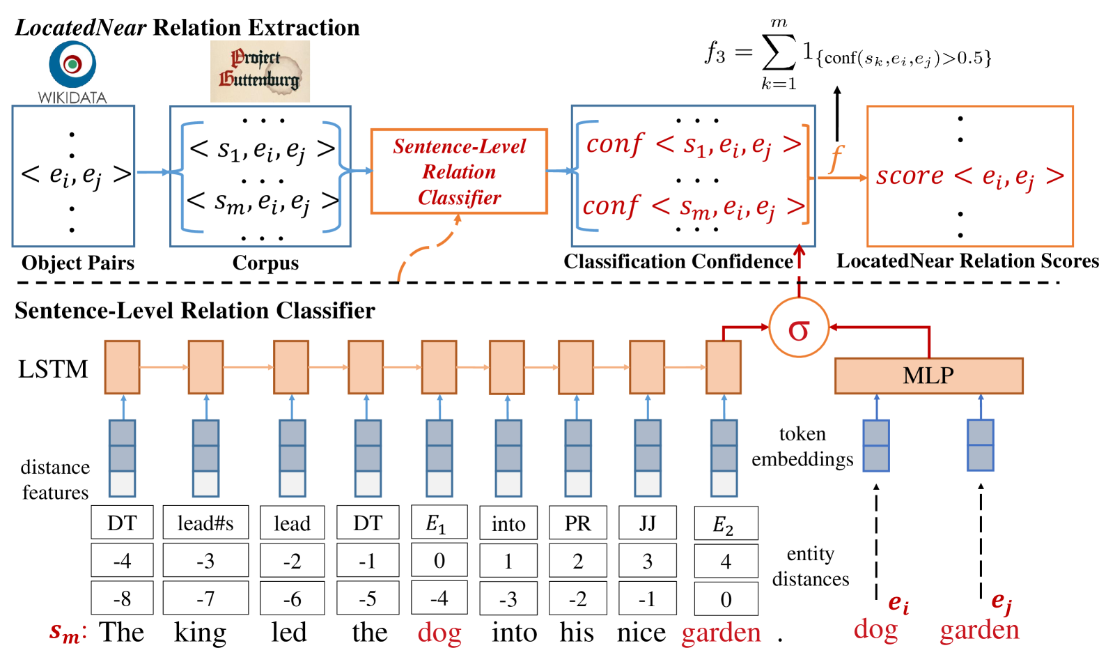
Figure 2: Framework with a LSTM-based classifier

2.2 LSTM-based Neural Architectures

We observe that the existence of LocatedNear relation in an instance <$s$,$e_{1}$,$e_{2}$>  depends on two major information sources: one is from the semantic and syntactical features of sentence $s$ and the other is from the object pair <$e_{1}$,$e_{2}$>. By this intuition, we design our LSTM-based model with two parts, shown in lower part of Figure 2. The left part is for encoding the syntactical and semantic information of the sentence $s$, while the right part is encoding the semantic similarity between the pre-trained word embeddings of $e_{1}$ and $e_{2}$.

Solely relying on the original word sequence of a sentence $s$ has two problems: (i) the irrelevant words in the sentence can introduce noise into the model; (ii) the large vocabulary of original sentences induce too many parameters, which may cause over-fitting. For example, given two sentences “The king led the dog into his nice garden.” and “A criminal led the dog into a poor garden.”. The object pair is <dog, garden> in both sentences. The two words “lead” and “into” are essential for determining whether the object pair is located near, but they are not attached with due importance. Also, the semantic differences between irrelevant words, such as “king” and “criminal”, “beautiful” and “poor”, are not useful to the co-location relation between the “dog” and “garden”, and thus tend to act as noise.

Level	Examples
Objects	$\textnormal{E}_{1}$, $\textnormal{E}_{2}$
Lemma	open, lead, into, …
Dependency Role	open#s, open#o, into#o, …
POS Tag	DT, PR, CC, JJ, …

Table 1: Examples of four types of tokens during sentence normalization. (#s stands for subjects and #o for objects)

To address the above issues, we propose a normalized sentence representation method merging the three most important and relevant kinds of information about each instance: lemmatized forms, POS (Part-of-Speech) tags and dependency roles. We first replace the two nouns in the object pair as “$\textnormal{E}_{1}$” and “$\textnormal{E}_{2}$”, and keep the lemmatized form of the original words for all the verbs, adverbs and prepositions, which are highly relevant to describing physical scenes. Then, we replace the subjects and direct objects of the verbs and prepositions (nsubj, dobj for verbs and case for prepositions in dependency parse trees) with special tokens indicating their dependency roles. For the remaining words, we simply use their POS tags to replace the originals. The four kinds of tokens are illustrated in  Table 1. Figure 2 shows a real example of our normalized sentence representation, where the object pair of interest is <dog, garden>.

Apart from the normalized tokens of the original sequence, to capture more structural information, we also encode the distances from each token to $\textnormal{E}_{1}$ and $\textnormal{E}_{2}$ respectively. Such position embeddings (position/distance features) are proposed by Zeng et al. (2014) with the intuition that information needed to determine the relation between two target nouns normally comes from the words which are close to the target nouns.

Then, we leverage LSTM to encode the whole sequence of the tokens of normalized representation plus position embedding. In the meantime, two pretrained GloVe word embeddings Pennington et al. (2014) of the original two physical object words are fed into a hidden dense layer.

Finally, we concatenate both outputs and then use sigmoid activation function to obtain the final prediction. We choose to use the popular binary cross-entropy as our loss function, and RMSProp as the optimizer. We apply a dropout rate Zaremba et al. (2014) of 0.5 in the LSTM and embedding layer to prevent overfitting.

3 LocatedNear  Relation Extraction

The upper part of Figure 2 shows the overall workflow of our automatic framework to mine LocatedNear relations from raw text. We first construct a vocabulary of physical objects and generate all candidate instances. For each sentence in the corpus, if a pair of physical objects $e_{i}$ and $e_{j}$ appear as nouns in a sentence $s$, then we apply our sentence-level relation classifier on this instance. The relation classifier yields a probabilistic score $s$ indicating the confidence of the instance in the existence of LocatedNear relation. Finally, all scores of the instances from the corpus are grouped by the object pairs and aggregated, where each object pair is associated with a final score. These mined physical pairs with scores can easily be integrated into existing commonsense knowledge base.

More specifically, for each object pair <$e_{i},e_{j}$>, we find all the $m$ sentences in our corpus mentioning both objects. We classify the $m$ instances with the sentence-level relation classifier and obtain confidence scores for each instance, then feed them into a heuristic scoring function $f$ to obtain the final aggregated score for the given object pair. We propose the following 5 choices of $f$ considering accumulation and threshold:

$$f_{0} =m$$ (1)

$$f_{1} =\sum_{k=1}^{m}\textnormal{conf}(s_{k},e_{i},e_{j})$$ (2)

$$f_{2} =\frac{1}{m}\sum_{k=1}^{m}\textnormal{conf}(s_{k},e_{i},e_{j})$$ (3)

$$f_{3} =\sum_{k=1}^{m}1_{\{\textnormal{conf}(s_{k},e_{i},e_{j})>0.5\}}$$ (4)

$$f_{4} =\frac{1}{m}\sum_{k=1}^{m}1_{\{\textnormal{conf}(s_{k},e_{i},e_{j})>0.5\}}$$ (5)

4 Datasets

Our proposed vocabulary of single-word physical objects is constructed by the intersection of all ConceptNet concepts and all entities that belong to “physical object” class in Wikidata Vrandečić and Krötzsch (2014). We manually filter out some words that have the meaning of an abstract concept, which results in 1,169 physical objects in total.

Afterwards, we utilize a cleaned subset of the Project Gutenberg corpus Lahiri (2014), which contains 3,036 English books written by 142 authors. An assumption here is that sentences in fictions are more likely to describe real life scenes. We sample and investigate the density of LocatedNear  relations in Gutenberg with other widely used corpora, namely Wikipedia, used by Mintz et al. (2009) and New York Times corpus Riedel et al. (2010). In the English Wikipedia dump, out of all sentences which mentions at least two physical objects, 32.4% turn out to be positive. In the New York Times corpus, the percentage of positive sentences is only 25.1%. In contrast, that percentage in the Gutenberg corpus is 55.1%, much higher than the other two corpora, making it a good choice for LocatedNear  relation extraction.

From this corpus, we identify 15,193 pairs that co-occur in more than 10 sentences. Among these pairs, we randomly select 500 object pairs and 10 sentences with respect to each pair for annotators to label their commonsense LocatedNear. Each instance is labeled by at least three annotators who are college students and proficient with English. The final truth labels are decided by majority voting. The Cohen’s Kappa among the three annotators is 0.711 which suggests substantial agreement Landis and Koch (1977). This dataset has almost double the size of those most popular relations in the SemEval task Hendrickx et al. (2010), and the sentences in our data set tend to be longer. We randomly choose 4,000 instances as the training set and 1,000 as the test set for evaluating the sentence-level relation classification task. For the second task, we further ask the annotators to label whether each pair of objects are likely to locate near each other in the real world. Majority votes determine the final truth labels. The inter-annotator agreement here is 0.703 (substantial agreement).

5 Evaluation

	Random	Majority	SVM	SVM(-BW)	SVM(-BPW)	SVM(-BAP)	SVM(-GF)
Acc.	0.500	0.551	0.584	0.577	0.556	0.563	0.605
P	0.551	0.551	0.606	0.579	0.567	0.573	0.616
R	0.500	1.000	0.702	0.675	0.681	0.811	0.751
F1	0.524	0.710	0.650	0.623	0.619	0.672	0.677
	SVM(-SDP)	SVM(-SS)	DRNN	LSTM+Word	LSTM+POS	LSTM+Norm
Acc.	0.579	0.584	0.635	0.637	0.641	0.653
P	0.597	0.605	0.658	0.635	0.650	0.654
R	0.728	0.708	0.702	0.800	0.751	0.784
F1	0.656	0.652	0.679	0.708	0.697	0.713

Table 2: Performance of baselines on co-location classification task with ablation. (Acc.=Accuracy, P=Precision, R=Recall, “-” means without certain feature)

In this section, we first present our evaluation of our proposed methods and the state-of-the-art general relation classification model on the first task. Then, we evaluate the quality of the new LocatedNear triples we extracted.

5.1 Sentence-level LocatedNear Relation Classification

We evaluate the proposed methods against the state-of-the-art general domain relation classification model (DRNN) Xu et al. (2016). The results are shown in Table 2. For feature-based SVM, we do feature ablation on each of the 6 feature types. For LSTM-based model, we experiment on variants of input sequence of original sentence: “LSTM+Word” uses the original words as the input tokens; “LSTM+POS” uses only POS tags as the input tokens; “LSTM+Norm” uses the tokens of sequence after sentence normalization. Besides, we add two naive baselines: “Random” baseline method classifies the instances into two classes with equal probability. “Majority” baseline method considers all the instances to be positive.

From the results, we find that the SVM model without the Global Features performs best, which indicates that bag-of-word features benefit more in shortest dependency paths than on the whole sentence. Also, we notice that DRNN performs best (0.658) on precision but not significantly higher than LSTM+Norm (0.654). The experiment shows that LSTM+Word enjoys the highest recall score, while LSTM+Norm is the best one in terms of the overall performance. One reason is that the normalization representation reduces the vocabulary of input sequences, while also preserving important syntactical and semantic information. Another reason is that the LocatedNear relation are described in sentences decorated with prepositions/adverbs. These words are usually descendants of the object word in the dependency tree, outside of the shortest dependency paths. Thus, DRNN cannot capture the information from the words belonging to the descendants of the two object words in the tree, but this information is well captured by LSTM+Norm.

5.2 LocatedNear Relation Extraction

Once we have obtained the probability score for each instance using LSTM+Norm, we can extract LocatedNear relation using the scoring function $f$. We compare the performance of 5 different heuristic choices of $f$, by quantitative results. We rank 500 commonsense LocatedNear object pairs described in Section 3. Table 3 shows the ranking results using Mean Average Precision (MAP) and Precision at $K$ as the metrics. Accumulative scores ($f_{1}$ and $f_{3}$) generally do better. Thus, we choose $f=f_{3}$ with a MAP score of 0.59 as the scoring function.

${f}$	MAP	P@50	P@100	P@200	P@300
$f_{0}$	0.42	0.40	0.44	0.42	0.38
$f_{1}$	0.58	0.70	0.60	0.53	0.44
$f_{2}$	0.48	0.56	0.52	0.49	0.42
$f_{3}$	0.59	0.68	0.63	0.55	0.44
$f_{4}$	0.56	0.40	0.48	0.50	0.42

Table 3: Ranking results of scoring functions.

(door, room)	(boy, girl)	(cup, tea)
(ship, sea)	(house, garden)	(arm, leg)
(fire, wood)	(house, fire)	(horse, saddle)
(fire, smoke)	(door, hall)	(door, street)
(book, table)	(fruit, tree)	(table, chair)

Table 4: Top object pairs returned by best performing scoring function $f_{3}$

Qualitatively, we show 15 object pairs with some of the highest $f_{3}$ scores in Table 4. Setting a threshold of 40.0 for $f_{3}$, which is the minimum non-zero $f_{3}$ score for all true object pairs in the LocatedNear object pairs data set (500 pairs), we obtain a total of 2,067 LocatedNear relations, with a precision of 68% by human inspection.

6 Conclusion

In this paper, we present a novel study on enriching LocatedNear relationship from textual corpora. Based on our two newly-collected benchmark datasets, we propose several methods to solve the sentence-level relation classification problem. We show that existing methods do not work as well on this task and discovered that LSTM-based model does not have significant edge over simpler feature-based model. Whereas, our multi-level sentence normalization turns out to be useful.

Future directions include: 1) better leveraging distant supervision to reduce human efforts, 2) incorporating knowledge graph embedding techniques, 3) applying the LocatedNear knowledge into downstream applications in computer vision and natural language processing.

References

- Bowman et al. (2015) Samuel R. Bowman, Gabor Angeli, Christopher Potts, and Christopher D. Manning. 2015. A large annotated corpus for learning natural language inference. In Proceedings of the 2015 Conference on Empirical Methods in Natural Language Processing, pages 632–642. Association for Computational Linguistics.
- Dagan et al. (2009) Ido Dagan, Bill Dolan, Bernardo Magnini, and Dan Roth. 2009. Recognizing textual entailment: Rational, evaluation and approaches. Natural Language Engineering, 15(4):i–xvii.
- Hendrickx et al. (2010) Iris Hendrickx, Su Nam Kim, Zornitsa Kozareva, Preslav Nakov, Diarmuid Ó Séaghdha, Sebastian Padó, Marco Pennacchiotti, Lorenza Romano, and Stan Szpakowicz. 2010. Semeval-2010 task 8: Multi-way classification of semantic relations between pairs of nominals. In Proceedings of the 5th International Workshop on Semantic Evaluation, pages 33–38. Association for Computational Linguistics.
- Lahiri (2014) Shibamouli Lahiri. 2014. Complexity of word collocation networks: A preliminary structural analysis. In Proceedings of the Student Research Workshop at the 14th Conference of the European Chapter of the Association for Computational Linguistics, pages 96–105. Association for Computational Linguistics.
- Landis and Koch (1977) J. Richard Landis and Gary G. Koch. 1977. The measurement of observer agreement for categorical data. Biometrics, 33 1:159–74.
- Li et al. (2016) Xiang Li, Aynaz Taheri, Lifu Tu, and Kevin Gimpel. 2016. Commonsense knowledge base completion. In Proceedings of the 54th Annual Meeting of the Association for Computational Linguistics (ACL), Berlin, Germany, August. Association for Computational Linguistics, pages 1445–1455.
- Mintz et al. (2009) Mike Mintz, Steven Bills, Rion Snow, and Daniel Jurafsky. 2009. Distant supervision for relation extraction without labeled data. In Proceedings of the Joint Conference of the 47th Annual Meeting of the ACL and the 4th International Joint Conference on Natural Language Processing of the AFNLP, pages 1003–1011. Association for Computational Linguistics.
- Pennington et al. (2014) Jeffrey Pennington, Richard Socher, and Christopher Manning. 2014. Glove: Global vectors for word representation. In Proceedings of the 2014 Conference on Empirical Methods in Natural Language Processing (EMNLP), pages 1532–1543. Association for Computational Linguistics.
- Riedel et al. (2010) Sebastian Riedel, Limin Yao, and Andrew McCallum. 2010. Modeling relations and their mentions without labeled text. Machine learning and knowledge discovery in databases, pages 148–163.
- Speer and Havasi (2012) Robert Speer and Catherine Havasi. 2012. Representing general relational knowledge in conceptnet 5. In Proceedings of the Eighth International Conference on Language Resources and Evaluation (LREC-2012). European Language Resources Association (ELRA).
- Vrandečić and Krötzsch (2014) Denny Vrandečić and Markus Krötzsch. 2014. Wikidata: A free collaborative knowledgebase. Communications of ACM, 57:78–85.
- Xu et al. (2016) Yan Xu, Ran Jia, Lili Mou, Ge Li, Yunchuan Chen, Yangyang Lu, and Zhi Jin. 2016. Improved relation classification by deep recurrent neural networks with data augmentation. In Proceedings of COLING 2016, the 26th International Conference on Computational Linguistics: Technical Papers, pages 1461–1470. The COLING 2016 Organizing Committee.
- Xu et al. (2015) Yan Xu, Lili Mou, Ge Li, Yunchuan Chen, Hao Peng, and Zhi Jin. 2015. Classifying relations via long short term memory networks along shortest dependency paths. In Proceedings of the 2015 Conference on Empirical Methods in Natural Language Processing, pages 1785–1794. Association for Computational Linguistics.
- Yatskar et al. (2016) Mark Yatskar, Vicente Ordonez, and Ali Farhadi. 2016. Stating the obvious: Extracting visual common sense knowledge. In Proceedings of the 2016 Conference of the North American Chapter of the Association for Computational Linguistics: Human Language Technologies, pages 193–198. Association for Computational Linguistics.
- Zaremba et al. (2014) Wojciech Zaremba, Ilya Sutskever, and Oriol Vinyals. 2014. Recurrent neural network regularization. arXiv preprint arXiv:1409.2329.
- Zeng et al. (2014) Daojian Zeng, Kang Liu, Siwei Lai, Guangyou Zhou, and Jun Zhao. 2014. Relation classification via convolutional deep neural network. In Proceedings of COLING 2014, the 25th International Conference on Computational Linguistics: Technical Papers, pages 2335–2344. Dublin City University and Association for Computational Linguistics.
- Zhu et al. (2014) Yuke Zhu, Alireza Fathi, and Li Fei-Fei. 2014. Reasoning about object affordances in a knowledge base representation. In European conference on computer vision, pages 408–424. Springer.