Behaviour of Charged Spinning Massless Particles

Abstract

We revisit the classical theory of a relativistic massless charged point particle with spin and interacting with an external electromagnetic field. In particular, we give a proper definition of its kinetic energy and its total energy, the latter being conserved when the external field is stationary. We also write the conservation laws for the linear and angular momenta. Finally, we find that the particle’s velocity may differ from $c$ as a result of the spin—electromagnetic field interaction, without jeopardizing Lorentz invariance.

E-mails: mblivan@gmail.com, bruno.lqg@gmail.com,
azurnasirpal@gmail.com, opiguet@pq.cnpq.br

Keywords: Lorentz symmetry; massless charged particle; spinning particle; relativistic particle.

1 Introduction

Although charged, massless particles have never been observed in the world of real particles, electrons in two-dimensional materials such as graphene behave as massless quasi-particles, i.e., they show an approximately linear relativistic dispersion relation, of the type $E\sim v_{\rm F}|{\bf p}|$. The velocity $v_{\rm F}\sim 10^{6}$ m/s is the Fermi velocity, depending on the microscopic properties of the material. It plays the role of the velocity of light for such a “mini-relativistic theory”. Moreover, beyond its (chiral) helicity, the quasi-electron possesses a quantum number, the “pseudo-spin”, which makes its wave function have four components and obey a massless Dirac equation. An introduction to the physics of graphene may be found in the reviews [1, 2].

The existence of this very special behaviour justifies a re-visitation of the extensive literature dedicated to the theory of a classical, punctual, relativistic, spinning particle [3]–[29], which may be massive or not, and charged or not, beginning with the pioneering work of Frenkel [3, 4]. The generally accepted formalism using odd Grassmann numbers in order to describe the spin degrees of freedom was introduced by Martin [6] and then developed by the authors of Refs. [7]–[17]. It was already recognized in Ref. [7, 8] that this is the most natural formalism, the Grassmann algebra turning itself to a Clifford algebra describing a spin one-half quantum particle upon canonical quantization. A formalism based on a supersymmetry localized on the world line of the particle, allowing for treating the massive as well as the massless particle, was introduced in Refs. [9]–[12]. The formalism based on a Grassmann algebra seems also to be the only known way to derive the dynamics of a classical spinning particle, massive or not, from an action principle, as already indicated via suggesting examples in Ref. [6]. Interaction with an external electromagnetic field is usually considered. Refs. [15, 20] also treat the case of an external gravitational field.

A complete treatment of a particle that is both charged and massless is still missing, although many results may be found in the literature quoted above. These concern above all the existence of an action principle. Our concern here is about the properties of the solutions of the dynamical equations and about the possible conservation laws, namely those of energy, linear momentum and angular momentum. Our first new result is that, in contrast with the case of the spinless particle, the behaviour of the particle with non-zero spin is drastically different what is expected from a massless particle: its velocity may be lower or higher than the velocity of light $c$ ($c=1$ throughout the paper). Moreover, this happens without conflict with Special Relativity (characterized by its fundamental parameter $c$): Lorentz covariance of the equations is always preserved. The second new result is about the conservation laws associated with the symmetry properties of the external field. In particular, the Noether procedure applied to the case of a stationary external field allows us to obtain a proper definition of energy for a massless interacting particle—a definition that had not seemed to exist in the literature, up to now.

In order to be able to give a realistic classical interpretation, in the final part of this paper, we introduce, following [13], spin variables $\Sigma_{\mu\nu}$ that are quadratic in the odd Grassmann variables $\psi_{\mu}$, treating the $\Sigma$ as real numbers, instead of even Grassmann numbers that would be nilpotent. The resulting equations of motion are no more derivable from an action. Moreover, they suffer incompatibilities, excepted for special external field configurations, e.g., for constant fields. It is for the latter configuration that we solve the equations, analytically or numerically, in order to gain some insight on the behaviours we mentioned above. We must recall that various sets of dynamical equations are presented in the literature, based on an action principle or not. We shall stick here to the set of equations derived in the Lagrangian formalism based on a Grassmann algebra as developed in [9]–[12].

We restrict the scope of the present paper to the interaction with an external electromagnetic field. The specific problem of the radiation field has been treated by the authors of Refs. [24]–[27].

The plan of the paper is the following. We begin in Section 2 with a complete study of the spinless case in order to make some basic points more transparent. In Section 3, we present the results for the spinning case, with a last subsection containing particular solutions of interest, and finish with our conclusions, together with a comparison with the known results for the massive particle.

2 The Spinless Relativistic Particle

The action for a classical spinless particle of mass $m$ of electric charge $q$ interacting with an electromagnetic field, given by the potential vector $A_{\mu}$, in four-dimensional Minkowski space-time may be written as the following integral on a time-like curve ${\cal C}$ parametrized by $\lambda$ [11, 12, 23]:

$${S[x,e]}=-\displaystyle{\int}_{\!\!\!{\cal C}}d\lambda\left(\dfrac{1}{2e(\lambda)}\dot{x}(\lambda)^{2}+\dfrac{e(\lambda)}{2}m^{2}+q\,\dot{x}^{\mu}(\lambda)A_{\mu}(x(\lambda))\right),$$ (1)

where $x^{\mu}(\lambda)$ are the coordinates of the particle’s position and $e(\lambda)$ a real function on the curve ${\cal C}$ parametrized by $\lambda$. Under (infinitesimal) reparametrizations $\lambda^{\prime}$ = $\lambda+\varepsilon(\lambda)$, the coordinates $x^{\mu}$ transform as scalars and $e$ as a scalar density of weight 1:

$$\delta x^{\mu}=\varepsilon\dot{x}^{\mu},\quad\delta e=\varepsilon\dot{e}+\dot{\varepsilon}e.$$ (2)

Under these transformations, the action is invariant up to boundary terms, and the equations of motion following from the variation of $x^{\mu}(\lambda)$,

$$\dfrac{d}{d\lambda}\left(\dfrac{\dot{x}_{\mu}}{e}\right)-qF_{\mu\nu}\dot{x}^{\nu}=0,$$ (3)

where

$$F_{\mu\nu}=\partial_{\mu}A_{\nu}-\partial_{\nu}A_{\mu},$$ (4)

and the constraint following from the variation of $e(\lambda)$,

$$\dfrac{\dot{x}^{\mu}\dot{x}_{\mu}}{e^{2}}=m^{2},$$ (5)

are covariant.

The propagation of a massless charged particle is described by the same action where $m$ is set to zero.

We observe that the constraint (5) is not completely independent of the equations of motion (3). Indeed, multiplying the latter by $\dot{x}^{\mu}/e$, we find that the left-hand side of this constraint is a constant:

$$\dfrac{d}{d\lambda}\left(\dfrac{\dot{x}^{\mu}\dot{x}_{\mu}}{e^{2}}\right)=0.$$ (6)

This means that it will be sufficient to impose it at some initial value of the parameter $\lambda$.

The solution of the constraint (5) differs qualitatively in the massive and in the massless case. These cases will be therefore treated separately in the following subsections.

The theory defined by the action (1) can be considered as a gauge theory in the one-dimensional space-time defined by the world line ${\cal C}$, the gauge invariance being that under reparametrizations (2) and the fields being the position coordinates $x^{\mu}(\lambda)$ and the “einbein” function $e(\lambda)$, the formers transforming as scalars and the latter as a density of weight 1.

One way to fix the gauge is to fix a value for the non-physical variable $e(\lambda)$. One equivalent way is to simply choose a particular parametrization, e.g., proper time or coordinate time. Then $e(\lambda)$ will be determined by either the constraint (5)—if $\dot{x}^{\mu}\dot{x}_{\mu}$ $\not=$ 0, i.e., in the massive case— or the equations of motion (3).

2.1 The Massive Case

Let us begin with the proper time parametrization $\lambda$ = $\tau$. The 4-velocity $\dot{x}^{\mu}$ then satisfies

$$\dot{x}^{2}=\dot{x}^{\mu}\dot{x}_{\mu}=1,$$

so that the constraint (5) solves for $e(\tau)$ as

$$e=1/m,$$

where we have chosen the positive solution. The equation of motion (3) then takes the familiar covariant form

$$m\ddot{x}_{\mu}-q\,F_{\mu\nu}\dot{x}^{\nu}=0,$$

where the second term is the relativistic expression for the Lorentz force.

In the time coordinate parametrization (the dot meaning now a time derivative), the 4-velocity takes the form $(\gamma,\gamma\dot{\bf x})$, with $\dot{\bf x}$ = ($\dot{x}^{i}$, $i=1,2,3$) and $\gamma$ = $1/\sqrt{1-\dot{\bf x}^{2}}$. The constraint (5) solves now as

$$\dfrac{1}{e}=m\gamma,$$ (7)

and the equations of motion (3) read

$$\begin{array}[]{l}m\dfrac{d}{dt}\gamma=q\bf{E}\cdot\dot{\bf x},\vspace{3pt}\\ m\dfrac{d}{dt}\left(\gamma\dot{\bf x}\right)=q(\bf{E}+\dot{\bf x}\times\bf{B}),\end{array}$$ (8)

where we have identified the electric and magnetic fields as

$${\bf E}=(F_{01},F_{02},F_{03}),\quad{\bf B}=(-F_{23},-F_{31},-F_{12}).$$ (9)

In the stationary case, defined by $\partial_{t}A_{\mu}=0$, we have a conserved energy obtained by integrating the first of Equation (8):

$${\cal E}=\dfrac{1}{e(t)}+qA_{0}(x(t))=m\gamma(t)+qA_{0}(x(t)),$$ (10)

where the integration constant ${\cal E}$ is the total energy.

2.1.1 Example

In the case of four-dimensional space-time of coordinates $t,\,x,\,y,\,z$, with constant fields $\bf E$ = $(0,E,0)$ and $\bf B$ = $(0,0,B)$, we can perform a first integration of Equation (8), obtaining

$$\begin{array}[]{l}m\gamma\dot{x}-qBy+C_{1}=0,\vspace{3pt}\\ m\gamma\dot{y}+qBx-qEt+C_{2}=0,\vspace{3pt}\\ m\gamma\dot{z}+C_{3}=0,\end{array}$$ (11)

$C_{1}$, $C_{2}$ and $C_{3}$ being integration constants.

2.2 The Massless Case

2.2.1 Equations of Motion

We are now going to investigate the main topics of this paper, i.e., the motion of a massless charged particle in an electromagnetic field. The action is given in Equation (1), with now $m=0$. The main difference with respect to the massive one is in the constraint obtained by varying the variable $e(\lambda)$ in the action: it now takes the form of the light-cone condition

$$\dot{x}^{\mu}\dot{x}_{\mu}=0,$$ (12)

and we see that, on the contrary of the massive case, it does not determine $e(\lambda)$.

The equations of motion are given by (3) for a general parametrization. There is of course no proper time parametrization; we shall use the coordinate time as a parameter, so that they take the form

$$\begin{array}[]{l}\dfrac{d}{dt}\left(\dfrac{1}{e}\right)=q\bf{E}\cdot\dot{\bf x},\vspace{3pt}\\ \dfrac{d}{dt}\left(\dfrac{\dot{\bf x}}{e}\right)=q(\bf{E}+\dot{\bf x}\times\bf{B}).\end{array}$$ (13)

The constraint (12) now reads

$${\sum_{i=1}^{3}}(\dot{x}^{i})^{2}=1.$$ (14)

This constraint (14) not being taken into account, we have four differential equations for four functions, $x^{i}(t)$ and $e(t)$, of second order in the $x$s and first order in $e$. Its solutions depend therefore on seven integration constants. six of them can be fixed by six boundary conditions, which may be chosen as six initial conditions at $t=0$:

$$x^{i}(0)=0,\ i=1,2,3,\quad(\dot{x}^{1}(0),\dot{x}^{2}(0),\dot{x}^{3}(0))=(v_{0x},v_{0y},v_{0z}).$$ (15)

Due to Equation (6), the constraint (12) will be satisfied if it is verified at $t=0$, i.e.,

$$(v_{0x})^{2}+(v_{0y})^{2}+(v_{0z})^{2}=1.$$ (16)

One of the integration constants remain free and will be discussed in Section 2.2.2.

2.2.2 Energy Equation

The main difference with respect to the massive case is that the einbein function $e(t)$ is no more determined by the constraint (5). Let us try to interpret it. Its evolution is determined, up to an integration constant, by the first of Equation (13). Restricting ourselves to the stationary case, where $\partial_{t}A_{\mu}=0$; hence, $\bf E$ = $\bf-\nabla A_{0}$, we see that this equation is a total time derivative, which yields

$${\cal E}=\dfrac{1}{e(t)}+qA_{0}(x(t)).$$ (17)

The second term being the potential energy, we interpret the integration constant ${\cal E}$ as the total energy of the particle, its “kinetic energy” being identified with $1/e(t)$. In order to understand better the physical meaning of this, let us normalize the electric potential—which in the stationary case is defined up to a constant—by

$$A_{0}(x(t))=-\displaystyle{\int}_{\!\!\!\!0}^{t}dt^{\prime}\,{\bf E}(x(t^{\prime}){\dot{\bf x}}(t^{\prime}).$$

In this situation, ${\cal E}$ = $1/e(0)$, which may be interpreted as the kinetic energy accumulated until the time $t=0$. We shall assume ${\cal E}$ to be positive:

$${\cal E}>0.$$ (18)

We may rewrite the second of Equation (13) as

$$\dfrac{d}{dt}\left(({\cal E}-qA_{0})\dot{\bf x}\right)=q(\bf{E}+\dot{\bf x}\times\bf{B})$$ (19)

and remark that the energy ${\cal E}$—an arbitrary parameter—contributes to the inertia of the particle: increasing the value of ${\cal E}$ implies more inertia.

2.2.3 Example of a Constant Electromagnetic Field

In order to get more insight for the motion of the massless particle, let us consider constant fields $\bf E$ = $(0,E,0)$ and $\bf B$ = $(0,0,B)$, orthogonal to each other. We can perform a first integration of Equation (19), obtaining

$$\begin{array}[]{l}({\cal E}+qEy)\dot{x}-qBy+C_{1}=0,\vspace{3pt}\\ ({\cal E}+qEy)\dot{y}+qBx-qEt+C_{2}=0,\vspace{3pt}\\ ({\cal E}+qEy)\dot{z}+C_{3}=0,\end{array}$$ (20)

where the energy (17) reads

$${\cal E}=\dfrac{1}{e(t)}-qEy(t).$$ (21)

The integration constants $C_{1}$, $C_{2}$ and $C_{3}$ are fixed as

$$C_{1}=-{\cal E}v_{0x},\quad C_{2}=-{\cal E}v_{0y},\quad C_{3}=-{\cal E}v_{0z},$$ (22)

with $\sum_{i}(v_{0}^{i})^{2}=1$, by the initial conditions (15).

A peculiar feature of the solutions of Equation (20) is a transition in their qualitative behaviour: for $|B|>|E|$, the trajectory is bounded in the $y$-direction, i.e., the direction of the electric field, whereas it is unbounded in the case $|B|<|E|$. In order to show this, let us solve the system (20) for $x$ and $y$:

$$\begin{array}[]{l}x(t)=\dfrac{E}{B}t+\dfrac{{\cal E}v_{0y}}{qB}-\dfrac{{\cal E}\dot{y}(B-Ev_{0x})}{qB(B-E\dot{x})},\\[8.53581pt] y(t)=\dfrac{{\cal E}(\dot{x}-v_{0x})}{q(B-E\dot{x})}.\end{array}$$ (23)

Since the velocity components are all bounded by 1 in absolute value, it is clear that, if $|B|$ $>$ $|E|$, the denominator of the expression for $y(t)$ never vanishes, then $y(t)$ remains bounded. However, $x(t)$ is asymptotically linear in $t$ and thus is unbounded (unless the electric field vanishes).

Solutions with $y(t)$ unbounded are those for $|B|$ $\leq$ $|E|$. This set includes the limiting case $|B|$ $=$ $|E|$, where one explicitly checks that $y(t)$ and $x(t)$ go asymptotically as $x\sim t$ and $y\sim t^{2/3}$, respectively, as $t$ $\to$ $\infty$, unless the initial velocity is transverse to the electric field: $(v_{0x},\,v_{0y},v_{0z})$ = $(1,\,0,\,0)$, in which case the solution of the equations—with the given initial conditions (15)—is $x(t)=t$, $y(t)=0$.

Analytic solutions are easy to find for pure electric field or pure magnetic field. The solution for $B=0,$ satisfying the boundary conditions (15), reads

$$\begin{array}[]{l}x(t)=\dfrac{v_{0x}}{\omega}\log\left(\dfrac{\sqrt{(\omega t)^{2}+2v_{0y}\omega t+1}+\omega t+v_{0y}}{(1+v_{0y})}\right),\\[8.53581pt] y(t)=\dfrac{1}{\omega}\left(\sqrt{(\omega t)^{2}+2v_{0y}\omega t+1}-1\right),\\[8.53581pt] z(t)=\dfrac{v_{0z}}{v_{0x}}x(t),\end{array}$$ (24)

with $\omega=qE/{\cal E}$, whereas the solution for $E=0$ with the same boundary conditions reads

$$\begin{array}[]{l}x(t)=\dfrac{1}{\Omega}\displaystyle{\biggl{(}}-v_{0y}(\cos(\Omega t)-1)+v_{0x}\sin(\Omega t)\displaystyle{\biggr{)}},\\[8.53581pt] y(t)=\dfrac{1}{\Omega}\displaystyle{\biggl{(}}v_{0x}(\cos(\Omega t)-1)+v_{0y}\sin(\Omega t)\displaystyle{\biggr{)}},\\[8.53581pt] z(t)=v_{0z}t,\end{array}$$ (25)

where $\Omega=qB/{\cal E}$. We didn’t find analytic solutions of the system (20) in the presence of both the electric and the magnetic fields, but a numerical analysis is summarized in Figures 1 and 2, where we have confined the movement to the plane $(x,y)$ by setting to zero the initial velocity component $v_{0z}$. Figure 1 displays the particle trajectory for four values of the ratio $B/E$: as expected, the one for $B>E$ is bounded in the $y$-direction, which is the direction of the electric field, and exhibits a drift in the orthogonal direction. On the other hand, the two trajectories for $B>E$ are unbounded in both directions. The dotted line corresponds to the limiting case $B=E$, which shows a similar behaviour. In the case of $B=0$, we have the trajectory equation

$$y(x)=-\frac{1}{\omega}+\frac{v_{0x}}{\omega}\cosh\left(\frac{x}{v_{0x}/\omega}+\mbox{sech}^{-1}(v_{0x})\right),$$

which is not the catenary curved observed in the case of a massive particle [5, 21], except if $v_{0x}=1$. See, in particular, p. 55 of [5]. Figure 2 displays the trajectories for three values of the total energy ${\cal E}$, showing clearly the increase of the inertia with increasing energy, for cases (a) of $B<E$ and (b) of $B>E$.

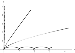
Figure 1: Particle trajectories in the $z=0$ plane for $0\leq t\leq 5$. Charge $q=1$, constant electric field $E$ in the positive $y$ direction, constant magnetic field $B$ in the positive $z$ direction. Energy ${\cal E}=0.2$, initial velocity ${\bf v}_{0}$ = $(0.1,0.995,0)$. Solid line: $B=1.6,\,E=1$; dotted line: $B=E=1$; dashed line: $B=0.4,\,E=1$; dotted-dashed line: $B=0,\,E=1$. The $B=0$ trajectory would be on the upper vertical axis in the case of ${\bf v}_{0}$ = $(0,1,0)$.

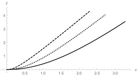
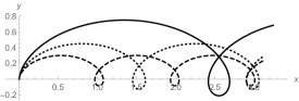
(a)	(b)

Figure 2: (a) particle trajectories in the $z=0$ plane for $0\leq t\leq 5$. Charge $q=1$, constant electric field $E=1$ in the positive $y$ direction, constant magnetic field $B=0.4$ in the positive $z$ direction. Initial velocity ${\bf v}_{0}$ = $(1,0,0)$. Dashed line: ${{\cal E}}=0.1$; dotted line: ${{\cal E}}=0.3$; solid line: ${{\cal E}}=0.7$; (b) Particle trajectories in the $z=0$ plane for $0\leq t\leq 5$. Charge $q=1$, constant electric field $E=1$ in the positive $y$ direction, constant magnetic field $B=1.6$ in the positive $z$ direction. Initial velocity ${\bf v}_{0}$ = $(0.1,0.995,0)$. Dashed line: ${\cal E}=0.2$; dotted line: ${\cal E}=0.3$; solid line: ${{\cal E}}=0.5$.

3 The Spinning Charged and Massless Particle

We turn now to the case of a spinning particle [13, 11, 12, 18, 19], completing action (1) by terms involving the spin degrees of freedom. The latter are described by Grassmann odd (i.e., anti-commuting) variables: a Lorentz vector $\psi^{\mu}(\lambda)$ and a scalar $\chi(\lambda)$. We restrict here to the less well established case of a massless particle. Recent accounts for the massive spinning particle may be found in [22, 23]

The manifestly Lorentz invariant action reads, as an integral along a curve $\mathcal{C}$ parametrized by $\lambda$ (We follow the conventions of [13]):

$$\begin{array}[]{l}S=-\displaystyle{\int}_{\!\!\!\mathcal{C}}d\lambda\displaystyle{\biggl{(}}\frac{1}{2e}\dot{x}^{\mu}\left(\dot{x}_{\mu}-i\chi\psi_{\mu}\right)+\dfrac{i}{2}\psi^{\mu}\dot{\psi}_{\mu}+qA_{\mu}\dot{x}^{\mu}-\dfrac{iq}{2}e\psi^{\mu}F_{\mu\nu}\psi^{\nu}\displaystyle{\biggr{)}},\end{array}$$ (26)

where a dot means a derivative with respect to $\lambda$.

The action (26) is invariant, up to boundary terms, under arbitrary reparametrizations of $\lambda$ and local supersymmetric transformations. With $\varepsilon(\lambda)$ (even) and $\alpha(\lambda)$ (odd) as infinitesimal parameters, these transformations read, respectively (The second term in the transformation of $\psi_{5}$, which does not appear in [13], is necessary and may be found in Equation (6.2) of [12]),

$$\begin{array}[]{l}\delta_{\varepsilon}x^{\mu}=\varepsilon\dot{x}^{\mu},\\[8.53581pt] \delta_{\varepsilon}e=\dot{\varepsilon}e+\varepsilon\dot{e},\\[8.53581pt] \delta_{\varepsilon}\psi^{\mu}=\varepsilon\dot{\psi}^{\mu},\\[8.53581pt] \delta_{\varepsilon}\chi=\dot{\varepsilon}\chi+\varepsilon\dot{\chi},\end{array}\begin{array}[]{l}\delta_{\alpha}x^{\mu}=i\alpha\psi^{\mu},\\[8.53581pt] \delta_{\alpha}e=-i\alpha\chi,\\[8.53581pt] \delta_{\alpha}\psi^{\mu}=-\alpha\left(\dot{x}^{\mu}-\frac{i}{2}\chi\psi^{\mu}\right)/e,\\[8.53581pt] \delta_{\alpha}\chi=2\dot{\alpha}.\end{array}$$ (27)

The electromagnetic potentials and fields then transform as

$$\begin{array}[]{l}\delta_{\varepsilon}A_{\mu}=\varepsilon\dot{A}_{\mu},\\[8.53581pt] \delta_{\varepsilon}F_{\mu\nu}=\varepsilon\dot{F}_{\mu\nu},\end{array}\begin{array}[]{l}\delta_{\alpha}A_{\mu}=i\alpha\partial_{\nu}A_{\mu}\psi^{\nu},\\[8.53581pt] \delta_{\alpha}F_{\mu\nu}=i\alpha\partial_{\rho}F_{\mu\nu}\psi^{\rho}.\end{array}$$ (28)

The commutator of two supersymmetry transformation yields the combination of a reparametrization and of a supersymmetry transformation:

$$[\delta_{\alpha},\delta_{\beta}]=\delta_{\tilde{\varepsilon}}+\delta_{\tilde{\alpha}},$$ (29)

with their infinitesimal parameters

$$\tilde{\varepsilon}=\frac{2i}{e}\alpha\beta,\qquad\tilde{\alpha}=-\frac{i\chi}{e}\alpha\beta.$$

Varying the action with respect to $e(\lambda)$ and $\chi(\lambda)$ yields the two constraints

$$C_{1}(\lambda):=\dfrac{\dot{x}^{\mu}\dot{x}_{\mu}}{e^{2}}-i\dfrac{\chi\dot{x}^{\mu}\psi_{\mu}}{e^{2}}+iq\psi^{\mu}F_{\mu\nu}\psi^{\nu}=0,$$ (30)

$$C_{2}(\lambda):=\dot{x}^{\mu}\psi_{\mu}=0.$$ (31)

We observe that the $\chi$-term in the bosonic constraint (30) vanishes due to the fermionic constraint (31).

The dynamical equations are obtained by varying the action with respect to $x^{\mu}(\lambda)$ and $\psi^{\mu}(\lambda)$:

$$\begin{array}[]{l}\dfrac{d}{d\lambda}\left(\dfrac{\dot{x}_{\mu}}{e}-i\dfrac{\chi\psi_{\mu}}{2e}\right)-q\left(\dot{x}^{\nu}F_{\mu\nu}-\dfrac{ie}{2}\psi^{\rho}\partial_{\mu}F_{\rho\sigma}\psi^{\sigma}\right)=0,\\[8.53581pt] \dot{\psi}_{\mu}+\dfrac{\dot{x}_{\mu}\chi}{2e}-eqF_{\mu\nu}\psi^{\nu}=0.\end{array}$$ (32)

The local supersymmetry transformation (27) for $\chi$ shows that the latter is a pure gauge of freedom, which will be set from now on to zero:

$$\chi=0.$$ (33)

This fixes the supersymmetry invariance. Later on, we will also fix reparametrization invariance by choosing a specific parametrization, namely $\lambda$ = $t$, instead of attributing a value to the einbein $e$ as is often done in the literature [9]–[20].

Using the dynamical Equation (32), the anticomutativity of the $\psi^{\mu}$’s and Equation (4), one shows that the left-hand sides of the constraints obey the equations

$$\dot{C}_{1}=0,\quad\quad\dfrac{\dot{C}_{2}}{C_{2}}=\dfrac{\dot{e}}{e}.$$ (34)

These are consistency conditions that show that constraints (30) and (31) are automatic consequences of the equations of motion (32) if they are satisfied for some initial value $\lambda_{0}$ of the evolution parameter.

The theory with Grassmann parameters just described is the appropriate one for an Hamiltonian formulation and a subsequent quantization, as it has been done for the free particle in [12, 16] and in [15, 20] with electromagnetic interaction, but only in the massive case. A theory easier to interpret as the one of a classical spinning particle may be obtained introducing the spin tensor $\Sigma$, whose components are even Grassmann numbers [13, 23]:

$$\Sigma_{\mu\nu}=-i\psi_{\mu}\psi_{\nu}=-\Sigma_{\nu\mu}.$$ (35)

This formulation is the one that is suitable as an effective theory, which ought to describe the semi-classical limit of the quantum theory in terms of expectation values.

The constraints (30) and (31) now read

$$\dfrac{\dot{x}_{\mu}\dot{x}^{\mu}}{e^{2}}-qF^{\mu\nu}\Sigma_{\mu\nu}=0,$$ (36)

$$\dot{x}^{\mu}\Sigma_{\mu\nu}=0,$$ (37)

and the equations of motion (32) take now the form

$$\dfrac{d}{d\lambda}\left(\dfrac{\dot{x}_{\mu}}{e}\right)-q\left(F_{\mu\nu}\dot{x}^{\nu}+\dfrac{e}{2}\partial_{\mu}F^{\rho\sigma}\Sigma_{\rho\sigma}\right)=0,$$ (38)

$$\dot{\Sigma}_{\mu\nu}-q\,e(F_{\mu}{}^{\sigma}\Sigma_{\sigma\nu}-F_{\nu}{}^{\sigma}\Sigma_{\sigma\mu})=0.$$ (39)

3.1 Time Parametrization

Choosing now the time parametrization, $\lambda$ = $t$, we see that the spin constraint (31) can be solved for the component $\psi_{0}$ in terms of the $\psi_{i}$ ($i=1,2,3$):

$$\psi_{0}=-\dot{x}^{i}\psi_{i},$$ (40)

where a dot now means the time derivative.

Instead of working with the odd Grassmann variables $\psi_{\mu}$, we shall use the even Grassmann spin tensor $\Sigma$ defined in Equation (35). Its components can be written as components of the two 3-vectors

$${\bf n}=(\Sigma_{01},\Sigma_{02},\Sigma_{03}),\quad{\bf s}=(\Sigma_{23},\Sigma_{31},\Sigma_{12}),$$ (41)

so that the spin constraint (37) can be solved for $\mathbf{n}$ in term of $\mathbf{s}$:

$$\mathbf{n}=\dot{\mathbf{x}}\times\mathbf{s},$$ (42)

and we observe that the vector $\mathbf{n}$ is orthogonal to the velocity. We remark that Equation (37) (or (42)) is identical to the covariant version of the Frenkel condition [3, 4, 23]—introduced for the massive case!—that the 3-vector $\bf n$ vanishes in the rest frame of the particle.

The constraint (36) and the dynamical equations for the position (38) read, respectively,

$$\dfrac{1-\dot{\mathbf{x}}^{2}}{e^{2}}+2q(\mathbf{s}\cdot\mathbf{B}+\mathbf{n}\cdot\mathbf{E})=0,$$ (43)

and

$$\begin{array}[]{l}\dfrac{d}{dt}\left(\dfrac{1}{e}\right)-q\mathbf{E}\cdot\dot{\mathbf{x}}+q\,e(\mathbf{s}\cdot\partial_{t}\mathbf{B}+\mathbf{n}\cdot\partial_{t}\mathbf{E})=0,\\[11.38109pt] \dfrac{d}{dt}\left(\dfrac{\dot{\mathbf{x}}}{e}\right)-q(\mathbf{E}+\dot{\mathbf{x}}\times\mathbf{B})-q\,e\sum_{i=1}^{3}(s_{i}\nabla B_{i}+n_{i}\nabla E_{i})=0.\end{array}$$ (44)

In the same way, the Equation (39) for the spin vector $\mathbf{s}$ reads

$$\dot{\mathbf{s}}+q\,e(\mathbf{E}\times\mathbf{n}+\mathbf{B}\times\mathbf{s})=0,$$ (45)

and the one for $\mathbf{n}$, $\dot{\mathbf{n}}+q\,e(\mathbf{B}\times\mathbf{n}-\mathbf{E}\times\mathbf{s})=0$, following from Equations (42) and (44).

N.B. We observe that the einbein variable $e(t)$ is dynamical, its evolution being defined by the first of Equation (44). On the other hand, the constraint (43) fixes the absolute value of the velocity, which may thus be variable and different from that of the light. This feature is a peculiarity of the massless theory. We will check this for some concrete examples in Section 3.4.

3.2 Conservation Laws

The first obvious conservation law is that of electric charge: the charge $q$ of the particle is just a parameter of the action defining the magnitude of the coupling with the external electromagnetic field.

Energy, momentum and angular momentum conservations, although not as trivial, are easily derived applying the Noether procedure. Their validities depend on the symmetries preserved by the external electromagnetic field.

In the case of a stationary exterior field, with $\partial_{t}A_{\mu}=0$, integration of the first of Equation (44) leads to the same conserved energy ${\cal E}$ as in the spinless case:

$${\cal E}=\dfrac{1}{e(t)}+qA_{0}(\mathbf{x(t)}).$$ (46)

Invariance under the space translations holds if the electromagnetic fields $\bf{E}$ and $\bf{B}$ are also constant in space, which is assured by the 4-potential vector $A_{\mu}$ = $f_{\mu\nu}x^{\nu}$, where the $f_{\mu\nu}$s are constants, antisymmetric in $\mu,\,\nu$. Then, this implies that the conservation of all four components of the energy-momentum 4 vector:

$${\cal P}_{\mu}=\dfrac{1}{e(t)}\dot{x}_{\mu}(t)-qf_{\mu\nu}x^{\nu}(t).$$ (47)

Finally, we have rotation invariance in a plane if the electric field vanishes and the magnetic field $\bf B$ points to a fixed direction. Choosing this direction to be the $z$ -axis, we deduce the conservation of the $z$ component of the total angular momentum:

$$J_{z}=-\dfrac{1}{e(t)}(\dot{x}(t)y(t)-\dot{y}(t)x(t))+\dfrac{qB}{2}(x^{2}(t)+y^{2}(t))+s_{z}(t),$$ (48)

the last term representing the spin part $s_{z}=-i\psi^{1}\psi^{2}$ (see definitions (35) and (41)).

3.3 Physical Interpretation of the Classical Theory

In order to be able to interpret the theory as a truly classical one, in terms of real numbers, one should forget about the Grassmann character of the spin variables $\Sigma_{\mu\nu}$ (or $\mathbf{s}$ and $\mathbf{n}$) and consider them as real number quantities. The theory would still be defined by the set of Equations (36)–(39), or (42)–(45) in the 3D notation. These equations do no more derive from an action principle, so that their consistency must be checked. Unfortunately, it happens that the spin constraint (37) is incompatible with the rest of the equations. Indeed, deriving it with respect to the evolution parameter $\lambda$,

$$\dfrac{d}{d\lambda}\left(\dot{x}^{\mu}\Sigma_{\mu\nu}\right)=\dfrac{q}{2}\partial^{\mu}F^{\rho\sigma}\Sigma_{\mu\nu}\Sigma_{\rho\sigma},$$ (49)

which only vanishes for special field configurations, such as, e.g., a constant electromagnetic field (If the $\Sigma^{\mu\nu}$s still were even Grassmann numbers, products of odd elements as in the definition (35), then the expression $\Sigma^{\mu\nu}\Sigma^{\rho\sigma}$ would be antisymmetric in the three indices $\mu,\rho,\sigma$ and the right-hand side of Equation (49) would vanish due to $F_{\rho\sigma}$ = $\partial_{\rho}A_{\sigma}-\partial_{\sigma}A_{\rho}$), which we shall consider in Section 3.4.

An alternative could be to use the constraint and equations of motion (36), the spin-constraint (37) or (42) on one hand, and the spin Equation (39) only for $\mu\nu$ = $ij$, i.e., for the spin 3-vector $\bf{s}$, on the other hand. However, such a choice would break Lorentz covariance.

3.4 Constant Electromagnetic Field

As we saw in the last subsection, the restriction to a constant electromagnetic field preserves the full set of the Lorentz covariant constraints and dynamical equations.

We shall consider the same configuration with a constant electromagnetic field as discussed in the spinless case at the end of Section 2.2.3, i.e., with $\bf{E}$ = $(0,E,0)$ and $\bf{B}$ = $(0,0,B)$, with mass zero and with the time parametrization, $\lambda=t$. The equations of motion for $e$, $x$, $y$ and $z$ take the same form (13), or their integrated form (20), as in the spinless case. The conserved energy is given by Equation (21). The constraint equation and the spin equations read

$$\dfrac{1-\dot{\mathbf{x}}^{2}}{e^{2}}+2q\left(Bs_{z}+E\dot{z}s_{x}-E\dot{x}s_{z}\right))=0,$$ (50)

$$\begin{array}[]{l}\dot{s}_{x}=q\,e\left(E\dot{y}s_{x}-E\dot{x}s_{y}+Bs_{y}\right),\\[8.53581pt] \dot{s}_{y}=-q\,eBs_{x},\\[8.53581pt] \dot{s}_{z}=q\,e\left(E\dot{y}s_{z}-E\dot{z}s_{y}\right).\end{array}$$ (51)

Solutions for $B=0$ or $E=0$ are easy to find. We use again the notations

$$\omega=\dfrac{qE}{{\cal E}},\quad\quad\Omega=\dfrac{qB}{{\cal E}},$$ (52)

of Section 2.2.3 and the boundary conditions (15).

For $B=0$, the evolution of the position coordinates is given by Equation (24), but with differences in the initial velocity components due to the modified constraint (see Equation (54)). The evolution of the spin components is given by

$$\begin{array}[]{l}s_{x}(t)=-\dfrac{s_{0y}v_{0x}(v_{0y}+\omega t)}{1-v_{0y}^{2}}+s_{0x}\sqrt{1+2v_{0y}\omega t+\omega^{2}t^{2}},\\[8.53581pt] s_{y}(t)=s_{0y},\\[8.53581pt] s_{z}(t)=-\dfrac{s_{0y}v_{0z}(v_{0y}+\omega t)}{1-v_{0y}^{2}}+s_{0z}\sqrt{1+2v_{0y}\omega t+\omega^{2}t^{2}}.\\[8.53581pt] \end{array}$$ (53)

The constraint reads

$${\cal E}(1-v_{0x}^{2}-v_{0y}^{2}-v_{0z}^{2})+2\omega(s_{0x}v_{0z}-s_{0z}v_{0x})=0.$$ (54)

In view of its constancy (see the first of Equation (34)), we have taken it at $t=0$: it is thus a constraint on the initial parameters $v_{0i}$ and $s_{0i}$. One sees that the particle’s velocity is not constrained to be equal to the velocity of light $c=1$—excepted for very peculiar initial spin/velocity configurations in which the spin part of Equation (54) vanishes. The particle’s velocity can even exceed $c$. We note that Lorentz invariance remains nevertheless unbroken. This feature, peculiar to the present approach of the classical massless spinning particle, will be encountered in various other examples, as we will see.

For the purely magnetic case, $E=0$, the position coordinates are given by Equation (25), and the spin components by the precession equations

$$\begin{array}[]{l}s_{x}(t)=s_{0x}\cos(\Omega t)+s_{0y}\sin(\Omega t),\\[8.53581pt] s_{y}(t)=s_{0y}\cos(\Omega t)-s_{0x}\sin(\Omega t),\\[8.53581pt] s_{z}(t)=s_{0z},\end{array}$$ (55)

where $(s_{0x},\,s_{0y},\,s_{0z})$ is the spin vector at $t=0$. The constraint reads

$${\cal E}(1-\dot{\mathbf{x}}^{2})+2\Omega s_{0z}=0.$$ (56)

One sees that the magnitude of the particle’s velocity—which here is constant due to the first of Equation (34)—can be higher or lower than the velocity of light, depending on the sign of $\Omega s_{0z}/{\cal E}$.

In the case of both $E$ and $B$ being non-zero, one has first to solve the constraint (50) for one of the velocity components, let us say the $x$-component. In view of the constancy of the constraint (see the first of Equation (34)), it is sufficient to do it at the initial time $t=0$ for the initial velocity component $v_{0x}$. It is thus a quadratic equation for the initial value of the velocity component, $v_{0x}$. In order to obtain real solutions, the discriminant

$$\Delta:=(1-v_{0y}^{2}-v_{0z}^{2}){\cal E}^{2}+2(s_{0x}v_{0z}\omega+s_{0z}\Omega){\cal E}+s_{0z}^{2}\omega^{2}$$ (57)

must be non-negative, hence the reality condition,

$$\Delta\geq 0,$$ (58)

must hold.

In order to be more explicit, we specialise from now on to the case of trajectories in the $(x,y)$-plane with the spin pointing to the $z$-direction, which is guaranteed by the initial conditions

$$v_{0z}=0,\quad\quad s_{0x}=s_{0y}=0.$$ (59)

The reality condition holds if and only if

$$v_{0y}^{2}\leq 1+\dfrac{2\Omega}{{\cal E}}s_{0z}+\dfrac{\omega^{2}}{{\cal E}^{2}}s_{0z}^{2}.$$ (60)

A necessary condition for this inequality is the positivity of the right-hand side, which holds in the following three cases:

$$\begin{array}[]{l}\mbox{(a) }|\omega|\geq|\Omega|,\quad\quad\quad\forall\,s_{0z},\\[8.53581pt] \mbox{(b) }|\omega|<|\Omega|,\quad\quad\quad s_{0z}<-\dfrac{{\cal E}\Omega}{\omega^{2}}-\dfrac{{\cal E}^{2}}{\omega^{2}}\sqrt{\dfrac{\Omega^{2}-\omega^{2}}{{\cal E}^{2}}},\\[8.53581pt] \mbox{(c) }|\omega|<|\Omega|,\quad\quad\quad s_{0z}>-\dfrac{{\cal E}\Omega}{\omega^{2}}+\dfrac{{\cal E}^{2}}{\omega^{2}}\sqrt{\dfrac{\Omega^{2}-\omega^{2}}{{\cal E}^{2}}}.\\[8.53581pt] \end{array}$$ (61)

Figure 3 shows some characteristic solutions.

(a) Trajectories in the $z=0$ plane.

(b) Spin $s_{z}(t)$.

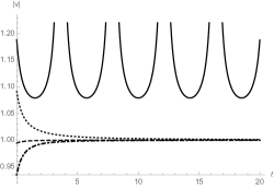
(c) Velocity $|\bf v(t)|$.

Figure 3: (a) Particle trajectories in the $z=0$ plane, (b) spin $s_{z}(t)$ and (c) velocity $|\bf v|$ = $|\dot{\mathbf{x}}(t)|$ for a constant electric field $E$ in the positive $y$ direction and a constant magnetic field $B$ in the positive $z$ direction. Parameters’ values are chosen as: charge $q=1$, energy ${\cal E}=2$, initial spin ${\bf s}(0)$ = $(0,0,0.5)$ and initial velocity ${\bf v}(0)$ = $(v_{0x},0.9,0)$, $v_{0x}$ being the largest of the solutions of the constraint (50). The following field configurations have been chosen: $B=3.2,\,E=2$ (solid lines); $B=E=2$ (dotted lines); $B=0.8,\,E=2$ (dashed lines); $B=0,\,E=2$ (dotted-dashed lines). The $B=0$ trajectory would be on the upper vertical axis in the case of ${\bf v}(0)$ = $(v_{0x},1,0)$.

One observes the same behaviour as in the spinless case for the trajectories (Figure 3a): bounded in the electric field direction (component $\dot{y}(t)$ for $|B|>|E|$, unbounded for $|B|\leq|E|$. A similar behaviour happens for the spin, as shown in Figure 3b: $s_{z}(t)$ is unbounded for $|B|\leq|E|$. In fact, all numerical examples investigated show this transition between bounded and unbounded behaviour happening both for $\dot{y}$ and $s_{z}$ at $|B|=|E|$. In Figure 3c, one sees the variation of the velocity’s absolute value in function of $t$. This velocity turns out to be always bounded.

4 Discussion and Conclusions

Our treatment of the massless charged particle in interactions with an external electromagnetic field led to two results, which, to the best of our knowledge, are new. One of them is the proper definition of energy given in Equation (17) for the spinless particle and in Equation (46) for the spinning one. In the time pametrization, the inverse of the einbein function, $1/e(t)$, plays the role of the “kinetic energy”. This was not recognized in the previous literature, where parametrization invariance is usually invoked in order to fix to some value the arbitrary function $e(\lambda)$.

The second result has been a non-constant particle’s absolute velocity, $|\mathbf{v}|$, different from $c$ in particular. It is interesting to compare with the massive particle case. For the massless particle, the result comes from the spin-electromagnetic field interaction present in the constraint (30). In the massive case, choosing the proper time parametrization (Dots now mean proper time derivative $d/d\tau$), where $\dot{x}^{2}=1$, we can solve this constraint for $e(\lambda)$:

$$\dfrac{1}{e}=m\sqrt{1+q\Sigma^{\mu\nu}F_{\mu\nu}/m^{2}},$$

with $\Sigma^{\mu\nu}$ defined by Equation (35). Combining with the energy equation

$${\cal E}=\dfrac{\dot{t}}{e}+qA_{0},$$

(deduced from the first of Equation (32) for $\mu=0$ in the stationary case), we obtain the time delay equation

$$\dfrac{d\tau}{dt}=\dfrac{m}{{\cal E}-qA_{0}}\sqrt{1+q\Sigma^{\mu\nu}F_{\mu\nu}/m^{2}},$$ (62)

a result similar to the one of [17], but not quite equal due to a different set of dynamical equations. An alternative theory for the massive particle has been very recently proposed in Refs. [28, 29], where a speed limit different from $c$ has been found, a result reinterpreted as a modification of the space-time metric. As said, these latter results are valid for the massive theory. The essential difference between the massive and the non-massive theories lies in the fact that, in the former case, the constraint may be solved for the einbein variable $e$, whereas, in the latter case, $e$ remains a dynamical variable—interpreted as the kinetic energy—and the constraint gives a (non-trivial) relation between the velocity components, as we have illustrated in specific examples.

We have considered both the pseudo-classical supersymmetric theory with odd Grassmann parameters, suitable for a canonical quantization, and the classical theory with spin described by real valued functions, which we have argued to better describe the classical limit of the quantum theory in terms of expectation values. The drawback of the latter description is the absence of an action principle and the incompatibility of the full system of equations excepted for special external field configurations, such as a constant one.

It is for a constant field configuration that we have calculated explicit solutions showing the characteristic behaviours of the particle, in particular the fact that, due to the interaction of the spin with the external field, its velocity is in general different from the velocity of light, without contradiction to Lorentz invariance.

Finally, let us comment that a speed higher than $c$ would of course generate a conflict with causality, as tachyons do, and may constitute an argument explaining the absence of such particles in the realm of fundamental physics. On the other hand, there would be no such problem in applications to condensed matter physics, such as graphene. There, the critical velocity $c$, taken equal to 1 in this paper and which plays the role of the relativistic “velocity of light”, is far smaller [1, 2] than the true velocity of light in the vacuum, the one which defines the causal structure of space-time.

As announced in the Introduction, our considerations are purely classical. Of course, some “correspondence principle” should hold such that, at the level of the quantum theory, the behaviour of the expectation values, e.g., of the velocity, should, in certain limiting cases, follow the classical behaviour discussed here. However, a check of this conjecture lies beyond the scope of the present work.

Acknowledgements

We would like to thank Alexei Deriglazov for pointing out to us the recent and interesting works of Refs. [28, 29]. This work was partially funded by the Conselho Nacional de Desenvolvimento Científico e Tecnológico—CNPq, Brazil (I.M., Z.O. and O.P.), to the Coordenação de Aperfeiçoamento de Pessoal de Nível Superior—CAPES, Brazil (I.M. and B.N.) and to the Grupo de Sistemas Complejos de la Carrera de Física de la Universidad Mayor de San Andrés, UMSA, for their support (Z.O.). B. N. would like to show his gratitude to Camila G. S. Moraes who immensely supported him during the course of this research.

References

- [1] Geim, A.K.; MacDonal, A.H. Graphene: Exploring carbon flatland. Phys. Today 2007, 60, doi:10.1063/1.2774096.
- [2] Castro, A.H.; Guinea, N.F.; Peres, N.M.P.; Novoselov, K.S.; Geim, A.K. The electronic properties of graphene. Rev. Mod. Phys. 2009, 81, 109.
- [3] Frenkel, J. Zur Elektrodynamik punktförmiger Elektronen. Z. Phys. 1925, 32, 518–534.
- [4] Frenkel, J. Die Elektrodynamik des Rotierenden Electrons. Z. Phys. 1926, 37, 243–262.
- [5] Landau, L.D.; Lifschitz, E.M. The Classical Theory of Fields. In Course of Theoretical Physics; Oxford-Pergamon Press: Oxford, UK, 1975; Volume 2.
- [6] Martin, J.L. Generalized Classical Dynamics and the ‘Classical Analogue’ of a Fermi Oscillator. Proc. R. Soc. Lond. A 1959, 251, 536.
- [7] Berezin, F.A.; Marinov, M.S. Classical Spin and Grassmann Algebra. Pisma Zh. Eksp. Teor. Fiz. 1975, 21, 678–680. (In Russian)
- [8] Berezin, F.A.; Marinov, M.S. Particle Spin Dynamics as the Grassmann Variant of Classical Mechanics. Ann. Phys. 1977, 104, 336–362.
- [9] Casalbuoni, R. Relativity and supersymmetries. Phys. Lett. B 1976, 62, 49.
- [10] Casalbuoni, R. The classical mechanics for Bose-Fermi systems. Nuovo Cimento A 1976, 33, 389–431.
- [11] Brink, L.; Deser, S.; Zumino, B.; Di Vecchia, P.; Howe, P. Local supersymmetry for spinning particles. Phys. Lett. B 1976, 64 435–438. Errata. Phys. Lett. B 1977, 64 488.
- [12] Brink, L. ; Di Vecchia, P.; Howe, P. A Lagrangian formulation of the classical and quantum dynamics of spinning particles. Nucl. Phys. B 1977, 118, 76–94.
- [13] Balachandran, A.P.; Salomonson, P.; Skagerstam, B.-S.; Winnberg, J.-O. Classical description of a particle interacting with a non-Abelian gauge field. Phys. Rev. D 1977, 15, 2308.
- [14] Salomonson, P. Sypersymmetric actions for spinning particles. Phys. Rev. D 1978, 18, 1868.
- [15] Carlos, G.A.P.; Teitelboim, C. Classical supersymmetric particles. J. Math. Phys. 1980, 21, 1863–1880.
- [16] Van Holten, J.W. Quantum theory of a massless spinning particle. Z. Phys. C 1988, 41, 497–504.
- [17] Van Holten, J.W. On the electrodynamics of spinning particles. Nucl. Phys. B 1991, 356, 3–26.
- [18] Fainberg, V.Y. ; Marshakov, A.V. Local Supersymmetry and Dirac Particle Propagator as a Path Integral. Nucl. Phys. B 1988, 306, 659–676.
- [19] Aliev, T.M.; Fainberg, V.Y.; Pak, N.K. Path integral for spin: A New approach. Nucl. Phys. B 1994, 429, 321–343
- [20] Geyer, B.; Dmitry, G.; Shapiro, I.L. Path integral and pseudoclassical action for spinning particle in external electromagnetic and torsion fields. Int. J. Mod. Phys. A 2000, 15, 3861–3876.
- [21] Bittencourt, J.A. Fundamentals of Plasma Physics, 3rd ed.; Springer: New York, NY, USA, 2004, doi:10.1007/978-1-4757-4030-1.
- [22] Rohrlich, F. Classical Charged Particles, 3rd ed.; World Scientific Publishing: Singapore, 2007.
- [23] Kosyakov, B. Introduction to the Classical Theory of Particles and Fields; Springer: Berlin/Heidelberg, Germany, 2007.
- [24] Kosyakov, B.P. Massless interacting particles. J. Phys. A 2008, 41, 465401.
- [25] Azzurli, F.; Lechner, K. The Lienard-Wiechert field of accelerated massless charges. Phys. Lett. A 2013, 377, 1025–1029, doi:10.1016/j.physleta.2013.02.046.
- [26] Azzurli, F.; Lechner, K. Electromagnetic fields and potentials generated by massless charged particles. Ann. Phys. 2014, 349, 1–32, doi:10.1016/j.aop.2014.06.005.
- [27] Lechner, K. Electrodynamics of massless charged particles. J. Math. Phys. 2015, 56, 022901, doi:10.1063/1.4906813.
- [28] Deriglazov, A.A.; Walberto, G.R. World-line geometry probed by fast spinning particle. Mod. Phys. Lett. A 2015, 30, 1550101.
- [29] Deriglazov, A.A.; Walberto, G.R. Ultrarelativistic Spinning Particle and a Rotating Body in External Fields.