Mobile Sensing of Two-Dimensional Bandlimited Fields on Random Paths

Abstract

Mobile sensing has been recently proposed for sampling spatial fields, where mobile sensors record the field along various paths for reconstruction. Classical and contemporary sampling typically assumes that the sampling locations are approximately known. This work explores multiple sampling strategies along random paths to sample and reconstruct a two dimensional bandlimited field. Extensive simulations are carried out, with insights from sensing matrices and their properties, to evaluate the sampling strategies. Their performance is measured by evaluating the stability of field reconstruction from field samples. The effect of location unawareness on some sampling strategies is also evaluated by simulations.

I Introduction

Sampling and reconstruction of two dimensional bandlimited fields (signals) is a well studied subject [1, 2]. Recently, mobile sensing was proposed for sampling spatial fields, where a mobile sensors records the field along various paths for reconstruction (interpolation) [3, 4, 5]. The sensing paths considered are mostly deterministic by construction. The main advantage of mobile sensing is a smaller number of sensing stations, at the cost of its mobility. Classical sampling and interpolation assumes that the sampling locations are (approximately) known [1, 2]. Of late, it has also been shown that a location-unaware mobile sensor can be used to estimate (reconstruct) a one-dimensional spatially bandlimited field [6].

With the above background, this work explores multiple sampling strategies along random paths to sample and reconstruct a spatially bandlimited field. These sampling strategies are compared and contrasted in this work. For location masking, sensors which average out the collected samples are also considered in some sampling strategies. A two-dimensional bandlimited (finite support) field has a finite number of non-zero Fourier coefficients. These coefficients represent the degrees of freedom of the field. One common theme observed is that oversampling beyond the degree of freedom aids in random path based sampling strategies. The performance of these sampling strategies is evaluated using the stability of spatial field reconstruction from field samples.

The main result of this work is the design and evaluation of multiple strategies for a two-dimensional bandlimited field sampling along random paths. The answers are obtained by extensive simulations along with intuitive insights.

Prior art: Sampling and estimation of bandlimited spatial fields on equi-spaced parallel paths by mobile sensors is studied and the aliasing error and measurement-noise is analyzed by Unnikrishnan and Vetterli [3]. Performance of several trajectories for mobile sensing is discussed in [4, 5]. The performance metric used here is path density. Results from classical sampling theory [1, 2] provide schemes for sampling and estimating the field based on measurements of the field at a countable number of nonuniform collection of points like the one depicted in Fig. 1(a). Location unawareness is introduced in mobile sensing and distributed sensing for one dimensional field by Kumar [6, 7]. Observing a spatial field at a random location is akin to random sensing studied in compressed sensing [8]. Tools from compressed sensing, therefore, are useful in the understanding of random path based sampling schemes.

II Preliminaries

II-A Field model

It is assumed that $g(x,y)$ is the field of interest. It is two dimensional, continuous and bandlimited, and supported in $\mbox{Rect}[\vec{0},\vec{1}]:=[0,1]\times[0,1]$. Bandlimitedness implies that

$$g(x,y)=\sum_{k=-b}^{b}\sum_{l=-b}^{b}a[k,l]\exp(j2\pi(kx+ly)),$$ (1)

where $a[k,l]$ are the Fourier coefficients of $g(x,y)$. The field is assumed to be temporally fixed (or slowly varying). It is noted that the problem of estimating a static field with mobile sensor(s) is involved and deserves a first study. The bandwidth in $(x,y)$ dimensions is assumed to be equal for simplicity, and does not affect the main results obtained in the paper. The number of Fourier coefficients is denoted by $n:=(2b+1)^{2}$, and denotes the real degrees of freedom. Even though each Fourier coefficient is complex valued, since $g(x,y)$ is real valued, conjugate symmetry of $a[k,l]$ limits the number of real degrees of freedom to $n$. At least $n$ samples of the field are, therefore, required to reconstruct it.

II-B Sampling Schemes

In this work, eight sampling schemes are considered. They are sequentially described in Section III. Largely, two sampling schemes are considered: point based sampling and path based sampling. In point based sampling, samples at various locations are collected in an array. From (1), each sample $g(x,y)$ can be expressed as an inner product between $n$ Fourier coefficients and a complex vector. Thus, $m$ spatial field samples at $(x_{i},y_{i}),1\leq i\leq m$ are given by

$$\begin{bmatrix}g(x_{1},y_{1})\\ \vdots\\ g(x_{m},y_{m})\end{bmatrix} =\begin{bmatrix}X_{11}&X_{12}&\dots&X_{1n}\\ \vdots&\vdots&\ddots&\vdots\\ X_{m1}&X_{m2}&\dots&X_{mn}\end{bmatrix}\begin{bmatrix}a[-b,-b]\\ \vdots\\ a[b,b]\end{bmatrix},$$

$$\mbox{or }\vec{g} =X\vec{a}$$ (2)

where $X_{qr}=\exp(j2\pi(k_{r}x_{q}+l_{r}y_{q}))$. The matrix $X:=[X_{qr}]_{m\times n}$ will be termed as the sensing matrix. The column parameters $k_{r},l_{r}$ correspond to the Fourier phasors for various $(k,l)$ pairs. The number of columns is therefore $n$.

In path based sampling, the mobile sensor is an accumulator which averages all the measurements made over a path. Averaging is advantageous since it denoises the readings made, and also does not require location information of individual samples. Similar to (2), a sensing matrix can be formed. If the sensor samples at $(x_{i,1},y_{i,1}),\ldots,(x_{i,p_{i}},y_{i,p_{i}})$ on path $i$ with $p_{i}$ points, then the sensing matrix $X_{\text{avg}}$ has the following entries

$$X_{\text{avg},ir}=\dfrac{1}{p_{i}}\Big{(}\sum_{t=1}^{p_{i}}\exp\big{(}j2\pi(k_{r}x_{i,t}+l_{r}y_{i,t})\big{)}\Big{)}$$ (3)

where $k_{r},l_{r}$ are the values of $k,l$ corresponding to the $r^{\text{th}}$ column, as before.

Figure 1: The random paths used for spatial sampling are illustrated: (a) benchmark sampling scheme where points are uniformly scattered over the sensing region; (b) the random paths consist of straight lines from boundary to boundary; (c) the random paths are straight lines between interior points; (d) the random paths are random walks; (e) the random paths start at end at designated boundary points; (f) the random paths start and end at designated interior points; and, (g) the random paths originate and end at randomly scattered center points.

II-C Measurement-noise model

In this work, measurement-noise is modeled by an independent and identically distributed (i.i.d.) process having zero mean and finite variance. If $W(x_{1},y_{1}),W(x_{2},y_{2}),\ldots$ are the measurement-noise samples, then they are i.i.d. and independent of the field and the random path selected for sampling.

III Sampling Models

Eight different sampling models, used in simulations, are described in this section. This will help discover randomized sampling schemes from which a bandlimited field can be estimated, even when sampling locations are unknown and measurement-noise is present. Most schemes are based on nonuniform random walks (or simply, random walks).

III-A Uniformly scattered fixed location sensors

In this model, static sensors are realized at uniformly distributed locations in $\mbox{Rect}[\vec{0},\vec{1}]$ (see Fig. 1(a)). This static sampling model is well known in the literature for field reconstruction [2]. This model will give us the benchmark performance of random sampling for comparisons.

III-B Sampling on random straight line paths

Equispaced straight line paths for field sampling were introduced by Unnikrisnan and Vetterli [3]. Let ${\cal B}[\vec{0},\vec{1}]$ be the boundary of the region $\mbox{Rect}[\vec{0},\vec{1}]$. In this model, a random straight line is chosen by selecting two independent points $\vec{b}_{1}$ and $\vec{b}_{2}$ with the distribution Uniform$({\cal B}[\vec{0},\vec{1}])$. It is assumed that the mobile sensor samples from $\vec{b}_{1}$ to $\vec{b}_{2}$. The inter-sample spacings are chosen according to $D\sim\mbox{Uniform}(0,\gamma)$ distribution, where $\gamma>0$ controls the average sample spacing on the path (see Fig. 1(b)). With path angle $\theta$ with respect to $x$-axis, the $t$-th field sample on a path is observed at

$$x_{t+1}=x_{t}+d_{t}\cos(\theta),\quad y_{t+1}=y_{t}+d_{t}\sin(\theta).$$ (4)

If $p$ paths and an average $\Gamma$ samples/path are selected for sampling, then the sensing matrix in (2) will be of the size $\Gamma p\times n$. To avoid an underdetermined system in (2), $p>2b+1$ and $\Gamma\geq 2b+1$ will be selected.

III-C Averaging over random straight line paths

In this sampling model, a path and sampling locations are selected as in Section III-B. However, all the samples along the path are averaged out by the mobile sensor to conserve storage and mask sampling locations. If $m$ is the number of paths, then the sensing matrix in (3) is of size $m\times n$.

III-D Straight line path between two inner points

In this sampling model, a random straight line is chosen by selecting two independent points $\vec{b}_{1}$ and $\vec{b}_{2}$ according to a Uniform$(\mbox{Rect}[\vec{0},\vec{1}])$ distribution. The sensor averages samples over a path and traverses according to the rule in (4) (see Fig. 1(c)). If $m$ is the number of paths, the sensing matrix is of size $m\times n$ as in (3).

III-E Random walk

In this model, the mobile sensor starts at a point $\vec{b}_{1}$ chosen uniformly in ${\cal B}[\vec{0},\vec{1}]$. Then, the sensor traverses at each step using a random step-size $D\sim\text{Uniform}(0,\gamma)$ and an angle $\theta\sim\text{Uniform}(0,2\pi)$. Sampling locations on the path are given by (4) with $\theta_{t}$ instead of $\theta$ (see Fig. 1(d)). In this model, the sensor may exit the boundary close to $\vec{b}_{1}$. For small $\gamma$, the sensor may sample at a large number of points as well.

III-F Directed random walk between boundary points

In this model, two independent points $\vec{b}_{1}$ and $\vec{b}_{2}$ are selected according to a Uniform$({\cal B}[\vec{0},\vec{1}])$ distribution. Path with end points on the same edge of the boundary are rejected. A random walk with $p$ steps is used to create a directed random walk from $\vec{b}_{1}$ to $\vec{b}_{2}$. The $p$-step random walk is implemented according to (4) and $(x_{1},y_{1})=\vec{b}_{1}$. Then to ensure the random walk is directed, the points are modified as

$$(x^{\prime}_{t},y^{\prime}_{t})=(x_{t},y_{t})+\frac{t}{p}(\vec{b}_{2}-(x_{p},y_{p}))$$ (5)

with $1\leq t\leq p$. Note that $(x^{\prime}_{1},y^{\prime}_{1})=\vec{b}_{1}$ and $(x^{\prime}_{p},y^{\prime}_{p})=\vec{b}_{2}$. These paths are illustrated in Fig. 1(e) and are inspired from Brownian motion and Brownian bridge [9].

III-G Directed random walk between two inner points

In this model, two independent points, $\vec{b}_{1}$ and $\vec{b}_{2}$ distributed according to Uniform$(\mbox{Rect}[\vec{0},\vec{1}])$ are generated. A directed random walk using the setup in (5) is generated (see Fig. 1(f)).

III-H Bee and hive sampling model

In this model, a point $\vec{b}_{c}$ is selected according to Uniform$(\mbox{Rect}[\vec{0},\vec{1}])$ distribution. The mobile sensor starts and ends its random walk at $\vec{b}_{c}$ using the setup in (5). A total of $m$ such points are generated. This sampling model is inspired by bees that hover around their hive and then return to the same location. The sensor is assumed to be location unaware. This sensing matrix will be of size $m\times n$.

IV Spatial field estimation method

The general method of reconstruction is explained. Since linear measurements are obtained, a regression based reconstruction is natural. From the samples collected by the mobile sensors (as described in Section III), a regression style estimate of Fourier coefficients $a[k,l]$ are obtained as follows:

$$\widehat{\vec{a}}=(X^{*}X)^{-1}X^{*}\vec{g}:={\cal Y}\vec{g}$$ (6)

where $\vec{g}$ are the field samples obtained either by taking samples or their averages along a path, and $X$ is the sensing matrix (see (2)).

If the sensor is location unaware, the sensing matrix is $X_{\text{un}}$, which is formed by approximating the locations using the end-points $\vec{b}_{1},\vec{b}_{2}$ of the path and the number $p$ of measurements made. The locations are approximated as

$$(x_{t},y_{t})_{\text{un}}=\vec{b}_{1}+\dfrac{t}{p-1}(\vec{b}_{2}-\vec{b}_{1}),\quad t=0,1,\ldots,p-1.$$ (7)

See Section V for the effect of location unawareness.

To test the feasibility of sampling, the stability of pseudo inverse in (6) has to be characterized. Analysis of the stability is very difficult for all the sampling schemes presented. So, we will adopt a simulation based approach. The stability of pseudo-inverse will be quantified using the condition number $C$ of a matrix. If samples are quantized or affected by independent measurement-noise, then a small condition number ensures that the estimate $\widehat{\vec{a}}$ is not too noisy. An ill-posed problem gives an unstable inverse and has a very high condition number. The condition number is defined as [8]

$$C_{2}(X)=\frac{\sigma_{\text{max}}(X)}{\sigma_{\text{min}}(X)}=\Big{(}\frac{\lambda_{\text{max}}(X^{*}X)}{\lambda_{\text{min}}(X^{*}X)}\Big{)}^{\frac{1}{2}}$$ (8)

where $\sigma$ and $\lambda$ denote the singular and eigenvalues, respectively. The condition number in our simulations depends on number of samples/paths $m$, the step-size parameter $\gamma$, and the location awareness/unawareness of sensor. The results are discussed next.

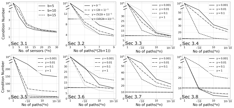
Figure 2: Condition number plots for various strategies are illustrated. The parameters $m$ and step-size $\gamma$ are varied. For uniformly scattered non mobile sensors, the variation is shown for different values of bandwidth parameter, $b$, and for the rest $b=10$ is fixed. These results are obtained by averaging over 50 iterations. The smallest condition numbers are achieved by schemes of Sec. 3.2 and Sec. 3.8.

V Results

The condition number corresponding to various sampling models in Section III are presented. These results are obtained by averaging $C_{2}(X)$ over 50 iterations. For computational efficiency in determining $C_{2}(X)$, the eigenvalues of $X^{*}X$ are calculated as it is a smaller matrix than $X$ (see (8)). As noted earlier, a low condition number is more desirable. The number of rows $m$ in the sensing matrix $X$ is always taken to be $\geq n=(2b+1)^{2}$ since it is necessary for the pseudo-inverse of $X$ to exist. So, the number of samples (or paths) is a multiple of $(2b+1)^{2}$ along the $x$-axis. All the results are illustrated in Fig. 2 and the plots are explained next.

A common trend is that with increasing size of sensing matrix $m$ the condition number improves. The benchmark sampling method in Sec. III-A achieves a condition number lower than $10$ for moderate values of $m$. The benchmark is the best performance to hope for, in terms of condition number. The results for sampling models in Sec. III-B and Sec. III-H are the best among random sampling strategies and near to the benchmark performances. This is especially surprising for Sec. III-H where the location information of sensor is also unknown. The schemes of Sec. III-C and Sec. III-F which operate with paths starting and ending at the boundary are fair; while, their counterparts in Sec. III-D and Sec. III-G with interior boundary points are average in performance. The worst scheme is of Sec. III-E, which consists of a fully random walk.

The condition number trends for all the schemes except Sec. III-B can be explained using condition number results from random matrix theory. From [8], it is known that if $X$ is an $m\times n$ sensing matrix with independent and sub-Gaussian rows, then for every $t>0$ with probability $\geq 1-e^{(-ht^{2})}$

$$1\leq\frac{\sigma_{\text{max}}(X)}{\sigma_{\text{min}}(X)}=C_{2}(X)\leq\frac{\sqrt{m}+H\sqrt{n}+t}{\sqrt{m}-H\sqrt{n}-t},$$ (9)

where $h,H>0$ are finite constants that depend only on the sampling model and not on $(n,m)$. So, condition number $C_{2}(X)$ provably improves with $m$.

As step-size $\gamma$ decreases, location unawareness of mobile sensors can also be introduced. Loosely speaking, as the average sampling rate over a straight line path increases, a random distribution of the points on the path averages to the equispaced points [6]. Therefore, the sensing matrix $X_{\text{un}}$ can be approximated as in (7). This is applicable to schemes in Sec. III-B, Sec. III-C, and Sec. III-D. In scheme of Sec. III-H, location-unawareness works since spatial field’s variation gets averaged out over the random walk for small step-size $\gamma$.

Finally, as the number of rows of sensing matrix $X$ increases, measurement-noise filtering naturally happens by regression in (6). A small condition number also ensures that measurement-noise power is less amplified [10].

VI Conclusions

Multiple sampling strategies along random paths to sample and reconstruct a two dimensional bandlimited field were explored. Using simulations it was found that a bee and hive based location-unaware random sampling design has the best condition number among various random sampling strategies. A close second is random straight-lines based sampling strategy. Most of the obtained results can be explained by using the condition number results from random matrix theory.

References

- [1] R. Marks, Introduction to Shannon Sampling and Interpolation Theory. New York: Springer-Verlag, 1991.
- [2] ——, Advanced Topics in Shannon Sampling and Interpolation Theory. New York: Springer-Verlag, 1993.
- [3] J. Unnikrishnan and M. Vetterli, “Sampling and reconstruction of spatial fields using mobile sensors,” IEEE Trans. Signal Proc., vol. 61, no. 9, pp. 2328–2340, May 2013.
- [4] ——, “Sampling high-dimensional bandlimited fields on low-dimensional manifolds,” IEEE Trans. Info. Theory, vol. 59, no. 4, pp. 2103–2127, 2013.
- [5] ——, “On optimal sampling trajectories for mobile sensing,” in Proceedings of the 10th International Conference on Sampling Theory and Applications, 2013, pp. 352–355.
- [6] A. Kumar, “On bandlimited field estimation from samples recorded by a location-unaware mobile sensor,” IEEE Trans. Info. Theory, vol. 63, no. 4, pp. 2188–2200, Jan. 2017.
- [7] ——, “On bandlimited signal reconstruction from the distribution of unknown sampling locations,” IEEE Trans. Signal Proc., vol. 63, no. 5, pp. 1259–1267, Mar. 2015.
- [8] Y. C. Eldar and G. K. (eds.), Compressed sensing. Theory and applications. Cambridge: Cambridge University Press, 2012.
- [9] R. Durrett, Brownian Motion and Martingales in Analysis. Wadsworth Pub Co, 1984.
- [10] P. J. Bickel and K. A. Doksum, Mathematical Statistics Vol I. Upper Saddle River, NJ, USA: Prentice Hall, 2001.