Single-particle properties of the Hubbard model
in a novel three-pole approximation

Abstract

We study the 2D Hubbard model using the Composite Operator Method within a novel three-pole approximation. Motivated by the long-standing experimental puzzle of the single-particle properties of the underdoped cuprates, we include in the operatorial basis, together with the usual Hubbard operators, a field describing the electronic transitions dressed by the nearest-neighbor spin fluctuations, which play a crucial role in the unconventional behavior of the Fermi surface and of the electronic dispersion. Then, we adopt this approximation to study the single-particle properties in the strong coupling regime and find an unexpected behavior of the van Hove singularity that can be seen as a precursor of a pseudogap regime.

1 Introduction

The Hubbard model [1, 2, 3], and its derivatives [4, 5] and extensions [6, 7, 8, 9], constitutes still one of the most studied model in condensed matter theory because of its relevance to almost all strongly correlated systems and, in particular, transition metal oxides. We report on a solution of the two-dimensional Hubbard model in the framework of the Composite Operator Method (COM) [10, 11, 12] within a novel three-pole approximation [12]. The COM, which is based on the equations of motion and Green’s function formalisms, is highly tunable and expressly devised for the characterization of strongly correlated electronic states and the exploration of novel emergent phases. Motivated by the long-standing experimental challenge posed by the puzzling single-particle properties of the underdoped cuprates [13, 14] (Fermi arcs, pseudogap, non-Fermi liquid behavior, extreme momentum dependence of spectral properties, …) , we adopt a basis of fields containing the two Hubbard operators and a third operator specifically designed to describe the electronic transitions dressed by the nearest-neighbor spin fluctuations and to capture the effects of these latter on all electronic properties. The spin fluctuations may play a crucial role in the mechanism of pseudogap formation and evolution as well as in the unconventional behavior of the Fermi surface, the spectral weights and the electronic dispersion [15, 16, 17]. Thus, we have designed this non canonical, but very efficient, operatorial representation of correlated electrons to provide a reliable analytical computational tool. The quality of this approximation has already been assessed positively by comparing its results against the numerical ones for many integrated/local quantities and for the band dispersion [12]. In this short paper, we adopt this approximation to study the single-particle properties of the model in the strong coupling regime, where the effects of the spin fluctuations, accurately treated in our approach, are more relevant and can induce unconventional features in all analyzed spectral properties. In particular, we find an unexpected behavior of the van Hove singularity only for high enough values of the on-site Coulomb repulsion that can be seen as a precursor of a pseudogap regime.

2 Model and method

The two-dimensional Hubbard model reads as

$$H =\sum_{\mathbf{i}}\left(-4tc^{\dagger}\left(i\right)\cdot c^{\alpha}\left(i\right)+Un_{\uparrow}\left(i\right)n_{\downarrow}\left(i\right)-\mu n\left(i\right)\right)$$ (1)

where $c^{\dagger}\left(i\right)=\begin{pmatrix}c_{\uparrow}^{\dagger}\left(i\right)&c_{\downarrow}^{\dagger}\left(i\right)\end{pmatrix}$ is the electronic field operator, in spinorial notation ($\cdot$ stands for the inner (scalar) product in spin space) and Heisenberg picture ($i=\left(\mathbf{i},t_{i}\right)$, being $\mathbf{i}=\mathbf{r_{i}}$ a Bravais lattice vector and $t_{i}$ the time), and $\sigma=\uparrow,\downarrow$ the electronic spin. $n_{\sigma}\left(i\right)=c_{\sigma}^{\dagger}\left(i\right)c_{\sigma}\left(i\right)$ is the particle density operator for spin $\sigma$ at site $\mathbf{i}$ and $n\left(i\right)=\sum_{\sigma}n_{\sigma}\left(i\right)=c^{\dagger}\left(i\right)\cdot c\left(i\right)$ is the total particle density operator at site $\mathbf{i}$. $c^{\alpha}\left(\mathbf{i},t\right)=\sum_{\mathbf{j}}\alpha_{\mathbf{ij}}c\left(\mathbf{j},t\right)$ where $\alpha_{\mathbf{ij}}=\dfrac{1}{2d}\delta_{\left\langle\mathbf{i}\mathbf{j}\right\rangle}$ is the nearest-neighbor projector. $U$ is the on-site Coulomb repulsion, $t$ is the nearest-neighbor hopping integral and $\mu$ is the chemical potential.

According the the COM recipe [11], we adopt a three-field basis

$$\Psi\left(i\right)=\left(\begin{array}[]{c}\psi_{1}\left(i\right)\\ \psi_{2}\left(i\right)\\ \psi_{3}\left(i\right)\end{array}\right)=\left(\begin{array}[]{l}\xi\left(i\right)=\left(1-n\left(i\right)\right)c\left(i\right)\\ \eta\left(i\right)=n\left(i\right)c\left(i\right)\\ c_{s}\left(i\right)=n_{k}\left(i\right)\sigma_{k}\cdot c^{\alpha}\left(i\right)\end{array}\right)$$ (2)

where $\eta\left(i\right)$ and $\xi\left(i\right)$ are the local Hubbard operators describing the transitions which change the electron numbers per site from 2 to 1 and from 1 to 0 respectively, and $c_{s}\left(i\right)$ describes the electronic transitions dressed by nearest-neighbor spin fluctuations, being $n_{k}\left(i\right)=c^{\dagger}\left(i\right)\cdot\sigma_{k}\cdot c\left(i\right)$ the spin density operator and $\sigma_{k}$ the Pauli matrices. We choose $c_{s}$ as third basis component according to the idea that the spin fluctuations are a key ingredient to describe strong correlations and they influence the dynamics more substantially than the other types of fluctuations (charge, pair, …). The operators $\psi_{n}$ are products of $c$ operators and, accordingly, they are composite operators. The vectorial current $J$ of the basis, $J\left(i\right)=i\dfrac{\partial}{\partial t}\Psi\left(i\right)=[\Psi\left(i\right),H]$, can be rewritten as $J\left(i\right)=\sum_{\mathbf{j}}\varepsilon\left(\mathbf{i},\mathbf{j}\right)\Psi\left(\mathbf{j},t\right)+\delta J\left(i\right)$, where the first term represents the operatorial projection of the current $J$ on the basis $\Psi$ and the second term is the residual current $\delta J$. The energy matrix $\varepsilon$ is obtained by means of the constraint $\left\langle\left\{\delta J\left(\mathbf{i},t\right),\Psi^{\dagger}\left(\mathbf{j},t\right)\right\}\right\rangle=0$, which assures that $\delta J$ retains only the physics orthogonal to the relevant one described by the chosen basis $\Psi$: $\varepsilon\left(\mathbf{k}\right)=m\left(\mathbf{k}\right)I^{-1}\left(\mathbf{k}\right)$. We have introduced, for the sake of simplicity, the $m$-matrix $m\left(\mathbf{i},\mathbf{j}\right)=\left\langle\left\{J\left(\mathbf{i},t\right),\Psi^{\dagger}\left(\mathbf{j},t\right)\right\}\right\rangle=\frac{1}{N}\sum_{\mathbf{k}}e^{i\mathbf{k\cdot\left(r_{i}-r_{j}\right)}}m\left(\mathbf{k}\right)$ and the normalization matrix $I\left(\mathbf{i},\mathbf{j}\right)=\left\langle\left\{\Psi\left(\mathbf{i},t\right),\>\Psi^{\dagger}\left(\mathbf{j},t\right)\right\}\right\rangle=\frac{1}{N}\sum_{\mathbf{k}}e^{i\mathbf{k\cdot\left(r_{i}-r_{j}\right)}}I\left(\mathbf{k}\right)$; $\left\langle...\right\rangle$ stands for the thermal average in the grand-canonical ensemble and $\mathbf{k}$ runs over the first Brillouin zone. $\varepsilon\left(\mathbf{k}\right)$, which is the Fourier transform of $\varepsilon\left(\mathbf{i},\mathbf{j}\right)$ – $\varepsilon\left(\mathbf{i},\mathbf{j}\right)=\frac{1}{N}\sum_{\mathbf{k}}e^{i\mathbf{k\cdot\left(r_{i}-r_{j}\right)}}\varepsilon\left(\mathbf{k}\right)$ –, has real eigenvalues $E^{\left(\nu\right)}\left(\mathbf{k}\right)$, which represent the excitation energy spectrum of the system, and its eigenvectors identify the elementary excitations of the system, within this approximation. We consider the thermal retarded Green’s function (GF) $G(\emph{i},\emph{j})=\langle\mathcal{R}\left[\Psi(\emph{i})\Psi^{\dagger}(\emph{j})\right]\rangle$ and its Fourier transform $G\left(\mathbf{k,\omega}\right)$, which can be obtained solving its Dyson’s equation in the frequency-momentum space (once the residual current is neglected)

$$G(\boldsymbol{k},\>\omega)=\dfrac{1}{\omega-\epsilon(\boldsymbol{k})+\mathrm{i}\delta}I(\boldsymbol{k})=\sum_{\nu}\dfrac{\sigma^{(\nu)}(\boldsymbol{k})}{\omega-E^{\left(\nu\right)}(\boldsymbol{k})+\mathrm{i}\delta}$$ (3)

$E^{\left(\nu\right)}(\boldsymbol{k})$ act as bands of the system and $\sigma^{\left(\nu\right)}\left(\mathbf{k}\right)$ are the matricial spectral density weights per band $\sigma_{mn}^{(\nu)}(\boldsymbol{k})=\sum_{c}\Omega_{m\nu}(\boldsymbol{k})\Omega_{\nu c}^{-1}(\boldsymbol{k})I_{cn}(\boldsymbol{k})$, where the matrix $\Omega\left(\mathbf{k}\right)$ has the eigenvectors of $\varepsilon\left(\mathbf{k}\right)$ as columns. The correlation functions of the fields of the basis $\Psi$, $C_{mn}\left(\mathbf{i},\mathbf{j}\right)=\left\langle\psi_{m}\left(\mathbf{i}\right)\psi_{n}^{\dagger}\left(\mathbf{j}\right)\right\rangle$, can be determined in terms of the GF by means of the spectral theorem

$$C_{mn}\left(\mathbf{k},\omega\right)=2\pi\sum\limits_{\nu}\left[1-f_{\mathrm{F}}\left(E^{\left(\nu\right)}\left(\mathbf{k}\right)\right)\right]\sigma_{mn}^{\left(\nu\right)}\left(\mathbf{k}\right)\delta\left(\omega-E^{\left(\nu\right)}\left(\mathbf{k}\right)\right)$$ (4)

where $f_{\mathrm{F}}$ is the Fermi function.

2.1 The equations of motion

The fields $\xi(i)$ and $\eta(i)$ satisfy the following equations of motion

$$\mathrm{i}\frac{\partial}{\partial t}\xi\left(i\right)=-\mu\xi\left(i\right)-4tc^{\alpha}\left(i\right)-4t\pi\left(i\right)$$ (5)

$$\mathrm{i}\frac{\partial}{\partial t}\eta\left(i\right)=\left(U-\mu\right)\eta\left(i\right)+4t\pi\left(i\right)$$ (6)

where $\pi\left(i\right)=\frac{1}{2}n_{\mu}(i)\sigma^{\mu}\cdot c^{\alpha}\left(i\right)+c^{\dagger\alpha}\left(i\right)\cdot c\left(i\right)\otimes c\left(i\right)$ is a higher-order composite field, $n_{\mu}\left(i\right)=c^{\dagger}\left(i\right)\cdot\sigma_{\mu}\cdot c\left(i\right)$ is the charge- ($\mu=0$) and spin- ($\mu=1,2,3=k$) density operator, $\sigma_{0}=\mathbf{1}$ is the identity matrix and $\otimes$ stands for the outer product in spin space. The field $c_{s}\left(i\right)$ satisfies the following equation of motion

$$\mathrm{i}\frac{\partial}{\partial t}c_{s}\left(i\right)=-\mu c_{s}\left(i\right)+4t\kappa_{s}\left(i\right)+U\eta_{s}\left(i\right)$$ (7)

where $\kappa_{s}\left(i\right)=\left(c^{\alpha\dagger}\left(i\right)\cdot\sigma_{k}\cdot c\left(i\right)-c^{\dagger}\left(i\right)\cdot\sigma_{k}\cdot c^{\alpha}\left(i\right)\right)\sigma_{k}\cdot c^{\alpha}\left(i\right)-n_{k}\left(i\right)\sigma_{k}\cdot c^{\alpha^{2}}\left(i\right)$, $\eta_{s}\left(i\right)=n_{k}\left(i\right)\sigma_{k}\cdot\eta^{\alpha}\left(i\right)$ and $c^{\alpha^{2}}\left(\mathbf{i},t\right)=\sum_{\mathbf{j}\mathbf{l}}\alpha_{\mathbf{ij}}\alpha_{\mathbf{j}\mathbf{l}}c\left(\mathbf{l},t\right)$.

2.2 The normalization matrix $I$

The normalization $I\left(\mathbf{k}\right)$ matrix is symmetric by construction and its entries have the following expressions

$$I_{11}\left(\mathbf{k}\right)=I_{11}=1-\frac{n}{2},\quad I_{12}\left(\mathbf{k}\right)=0,\quad I_{22}\left(\mathbf{k}\right)=I_{22}=\frac{n}{2}$$ (8)

$$I_{13}\left(\mathbf{k}\right)=3C_{\xi c}^{\alpha}+\frac{3}{2}\alpha\left(\mathbf{k}\right)\chi_{s}^{\alpha}$$ (9)

$$I_{23}\left(\mathbf{k}\right)=3C_{\eta c}^{\alpha}-\frac{3}{2}\alpha\left(\mathbf{k}\right)\chi_{s}^{\alpha}$$ (10)

$$I_{33}\left(\mathbf{k}\right)\cong 4C_{c_{s}c}^{\alpha}+\frac{3}{2}C_{\eta\eta}+3\alpha\left(\mathbf{k}\right)\left(f_{s}+\frac{1}{4}C_{cc}^{\alpha}\right)$$ (11)

where $n=\left\langle n\left(i\right)\right\rangle$ is the filling, $\chi_{s}^{\alpha}=\frac{1}{3}\sum_{k}\left\langle n_{k}^{\alpha}\left(i\right)n_{k}\left(i\right)\right\rangle$ is the nearest-neighbor spin-spin correlation function, $f_{s}=\frac{1}{3}\left\langle c^{\dagger}\left(i\right)\cdot\sigma_{k}\cdot c^{\alpha}\left(i\right)n_{k}^{\alpha}\left(i\right)\right\rangle$ is a higher-order (up to three different sites are involved) spin-spin correlation function, and $C_{mn}^{\alpha}=\left\langle\psi_{m}^{\alpha}\left(\mathbf{i}\right)\psi_{n}^{\dagger}\left(\mathbf{i}\right)\right\rangle$. Higher-order terms (involving more distant sites) in $I_{33}\left(\mathbf{k}\right)$ have been neglected [12].

2.3 The $m$-matrix

The $m\left(\mathbf{k}\right)$ matrix is symmetric by construction and its entries have the following expressions

$$m_{11}\left(\mathbf{k}\right)=-\mu I_{11}-4t\left[\Delta+\left(p+I_{11}-I_{22}\right)\alpha\left(\mathbf{k}\right)\right]$$ (12)

$$m_{12}\left(\mathbf{k}\right)=4t\left[\Delta+\left(p-I_{22}\right)\alpha\left(\mathbf{k}\right)\right]$$ (13)

$$m_{13}\left(\mathbf{k}\right)=-\left(\mu+4t\alpha\left(\mathbf{k}\right)\right)I_{13}\left(\mathbf{k}\right)-4t\alpha\left(\mathbf{k}\right)I_{23}\left(\mathbf{k}\right)-2tI_{33}\left(\mathbf{k}\right)-4t\gamma_{m}\alpha\left(\mathbf{k}\right)$$ (14)

$$m_{22}\left(\mathbf{k}\right)=\left(U-\mu\right)I_{22}-4t\left[\Delta+p\alpha\left(\mathbf{k}\right)\right]$$ (15)

$$m_{23}\left(\mathbf{k}\right)=\left(U-\mu\right)I_{23}\left(\mathbf{k}\right)+2tI_{33}\left(\mathbf{k}\right)+4t\gamma_{m}\alpha\left(\mathbf{k}\right)$$ (16)

$$m_{33}\left(\mathbf{k}\right)\cong-\mu I_{33}\left(\mathbf{k}\right)+m_{33}^{0r}+m_{33}^{\alpha r}\alpha\left(\mathbf{k}\right)$$ (17)

where $\Delta=C_{\xi\xi}^{\alpha}-C_{\eta\eta}^{\alpha}$, $p=\frac{1}{4}\left(\chi_{0}^{\alpha}+3\chi_{s}^{\alpha}\right)-\chi_{p}^{\alpha}$ is a combination of the nearest-neighbor charge-charge $\chi_{0}^{\alpha}=\left\langle n^{\alpha}\left(i\right)n\left(i\right)\right\rangle$, spin-spin $\chi_{s}^{\alpha}$ and pair-pair $\chi_{p}^{\alpha}=\left\langle\left[c_{\uparrow}\left(i\right)c_{\downarrow}\left(i\right)\right]^{\alpha}c_{\downarrow}^{\dagger}\left(i\right)c_{\uparrow}^{\dagger}\left(i\right)\right\rangle$ correlation functions, $\gamma_{m}$, $m_{33}^{0r}$, and $m_{33}^{\alpha r}$ are the combinations of many higher-order correlation functions [12]. Higher-order terms (involving more distant sites) in $m_{33}\left(\mathbf{k}\right)$ have been neglected [12].

2.4 Self-consistency and Algebra constraints

Algebra Constraints (ACs), exact relationship between the correlation functions of the fields of the chosen operatorial basis dictated by the non-canonical algebra they close, offer a very reliable way to fix unknown parameters and allow, at the same time, to impose to the system under analysis algebraic relations and/or symmetry requirements that are valid for any coupling and any value of the external parameters. In this case, we can recognize the following exact Algebra Constraints

$$C_{\xi\xi}=1-n+D,\quad C_{\xi\eta}=0,\quad C_{\eta\eta}=\frac{n}{2}-D$$ (18)

$$C_{\xi c_{s}}=3C_{\xi c}^{\alpha},\quad C_{\eta c_{s}}=0$$ (19)

where $D=\left\langle n_{\uparrow}\left(i\right)n_{\downarrow}\left(i\right)\right\rangle$ is the double occupancy. These relations lead to the following very relevant ones: $n=2\left(1-C_{\xi\xi}-C_{\eta\eta}\right)$ and $D=1-C_{\xi\xi}-2C_{\eta\eta}$. On the other hand, we can compute $\chi_{0}^{\alpha}$, $\chi_{s}^{\alpha}$, $\chi_{p}^{\alpha}$ and $f_{s}$ by operatorial projection [12]

$$\chi_{0}^{\alpha}\approx n^{2}-2\frac{I_{11}\left(C_{c\eta}^{\alpha}\right)^{2}+I_{22}\left(C_{c\xi}^{\alpha}\right)^{2}}{C_{\eta\eta}}$$ (20)

$$\chi_{s}^{\alpha}\approx-2\frac{I_{11}\left(C_{c\eta}^{\alpha}\right)^{2}+I_{22}\left(C_{c\xi}^{\alpha}\right)^{2}}{2I_{11}I_{22}-C_{\eta\eta}}$$ (21)

$$\chi_{p}^{\alpha}\approx\frac{C_{c\xi}^{\alpha}C_{\eta c}^{\alpha}}{C_{\eta\eta}}$$ (22)

$$f_{s}\approx-\frac{1}{2}C_{c\xi}^{\alpha}-\frac{3}{4}\chi_{s}^{\alpha}\left(\frac{C_{c\xi}^{\alpha}}{I_{11}}-\frac{C_{c\eta}^{\alpha}}{I_{22}}\right)$$

$$\quad-2\frac{C_{c\xi}^{\alpha}}{I_{11}}\left(C_{c\xi}^{\alpha^{2}}-\frac{1}{4}C_{c\xi}\right)-2\frac{C_{c\eta}^{\alpha}}{I_{22}}\left(C_{c\eta}^{\alpha^{2}}-\frac{1}{4}C_{c\eta}\right)$$ (23)

and use the three left ACs to compute $\gamma_{m}$, $m_{33}^{0r}$, and $m_{33}^{\alpha r}$.

3 Single-particle properties

We can now analyze the behavior of the single-particle properties of the system: energy bands, density of states and Fermi surface. In particular, we can study the energy bands of the system $E^{\left(\nu\right)}\left(\mathbf{k}\right)$ along the principal directions of the first Brillouin zone ($\Gamma=\left(0,0\right)\rightarrow S=\left(\pi/2,\pi/2\right)\rightarrow M=\left(\pi,\pi\right)\rightarrow X=\left(\pi,0\right)\rightarrow\Gamma=\left(0,0\right)$) as well as the corresponding electronic spectral density weight $\sigma_{cc}^{\left(\nu\right)}\left(\mathbf{k}\right)=\sum_{n,m=1}^{2}\sigma_{nm}^{\left(\nu\right)}\left(\mathbf{k}\right)$. This latter corresponds to the component per band of the momentum distribution function per spin $n\left(\mathbf{k}\right)$ at $T=0$ for those bands and momenta below the chemical potential. Giving to each energy band $E^{\left(\nu\right)}\left(\mathbf{k}\right)$ a thickness proportional to $\sigma_{cc}^{\left(\nu\right)}\left(\mathbf{k}\right)$ shows the effective relevance of each energy band, momentum per momentum, with respect to actual occupation and possible hole/electron doping. The density of states, $N\left(\omega\right)=\frac{1}{N}\sum_{\mathbf{k}}\sum_{\nu}\sigma_{cc}^{\left(\nu\right)}\left(\mathbf{k}\right)\delta\left(\omega-E^{\left(\nu\right)}\left(\mathbf{k}\right)\right)$, depends on both the electronic spectral weight, $\sigma_{cc}^{\left(\nu\right)}\left(\mathbf{k}\right)$, and the actual shape (through the curvature $\nabla_{\mathbf{k}}E^{\left(\nu\right)}\left(\mathbf{k}\right)$) of the bands

$$\delta\left(\omega-E^{\left(\nu\right)}\left(\mathbf{k}\right)\right)=\sum_{p}\frac{\delta\left(\mathbf{k}-\mathbf{k}_{p}^{\left(\nu\right)}\left(\omega\right)\right)}{\left|\nabla_{\mathbf{k}}E^{\left(\nu\right)}\left(\mathbf{k}\right)\right|_{\mathbf{k}=\mathbf{k}_{p}^{\left(\nu\right)}}}$$ (24)

where $\mathbf{k}_{p}^{\left(\nu\right)}\left(\omega\right)$ are the zeros of $\omega-E^{\left(\nu\right)}\left(\mathbf{k}\right)=0$. Finally, we can investigate the shape of the Fermi surface by means of the spectral function $A\left(\mathbf{k},\omega\right)=-\dfrac{1}{\pi}\Im\left[G_{cc}\left(\mathbf{k},\omega\right)\right]=\sum_{\nu}\sigma_{cc}^{\left(\nu\right)}\left(\mathbf{k}\right)\delta\left(\omega-E^{\left(\nu\right)}\left(\mathbf{k}\right)\right)$, where $G_{cc}\left(\mathbf{k}\right)=\sum_{n,m=1}^{2}G_{nm}\left(\mathbf{k}\right)$ is the electronic Green’s function. In fact, the position of the maxima of $A\left(\mathbf{k},\omega=0\right)$ provides the effective Fermi Surface as measured by ARPES (Angle Resolved Photo-Emission Spectroscopy) experiments. In all calculations, $\delta\left(\omega\right)$ has been replaced by a Lorentzian function $\dfrac{1}{\pi}\dfrac{\varepsilon}{\omega^{2}+\varepsilon^{2}}$ with $\varepsilon=0.05$.

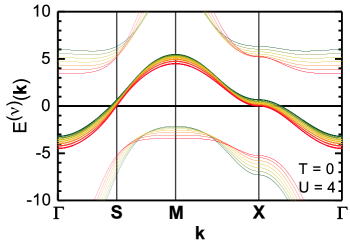
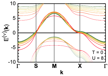
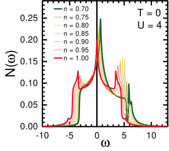
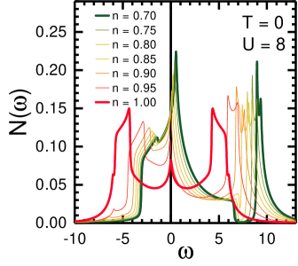
Figure 1: (top row) Energy bands $E^{\left(\nu\right)}\left(\mathbf{k}\right)$ along the principal directions of the first Brillouin zone ($\Gamma=\left(0,0\right)\rightarrow S=\left(\pi/2,\pi/2\right)\rightarrow M=\left(\pi,\pi\right)\rightarrow X=\left(\pi,0\right)\rightarrow\Gamma=\left(0,0\right)$) for $T=0$ and $U=4$ (left) and $U=8$ (right). The thickness of each band is proportional to the value of the corresponding electronic spectral density weight $\sigma_{cc}^{\left(\nu\right)}\left(\mathbf{k}\right)$. The different colors correspond to different values of the doping according to the legends in the bottom row. (bottom row) Density of states $N\left(\omega\right)$ for $T=0$ and $U=4$ (left) and $U=8$ (right). The different colors correspond to different values of the doping.

In Fig. 1, the energy bands $E^{\left(\nu\right)}\left(\mathbf{k}\right)$ along the principal directions of the first Brillouin zone ($\Gamma=\left(0,0\right)\rightarrow S=\left(\pi/2,\pi/2\right)\rightarrow M=\left(\pi,\pi\right)\rightarrow X=\left(\pi,0\right)\rightarrow\Gamma=\left(0,0\right)$) for $T=0$ and $U=4$ (top row, left panel) and $U=8$ (top row, right panel) are reported. The thickness of each band is proportional to the value of the corresponding electronic spectral density weight $\sigma_{cc}^{\left(\nu\right)}\left(\mathbf{k}\right)$. The different colors correspond to different values of the doping according to the legends in the bottom row. At the smaller value of $U$, $U=4$, the bands show a monotonous behavior on decreasing the doping down to half filling, $n=1$, where the central band crosses the chemical potential exactly along the main anti-diagonal ($X-S-Y=\left(0,\pi\right)$) as in the non-interacting case. The great majority of the weight is concentrated in the central band at all values of the filling and, just close to half filling, the other two bands acquire some non negligible weight for the momenta closer to the chemical potential. For the same momenta, these two bands become almost completely flat. For the higher value of $U$, $U=8$, the behavior is dramatically different at all momenta and, in particular, at the $M$ point where the curves do not follow anymore a monotonous behavior. The weights of the two non-central bands result much higher, in particular, close to half filling, where the first van Hove singularity (vHs) crossing seems to happen for a value of doping smaller than $n=1$.

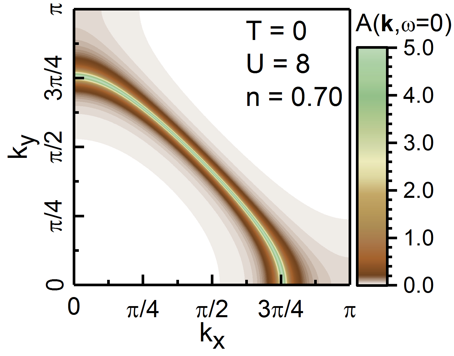
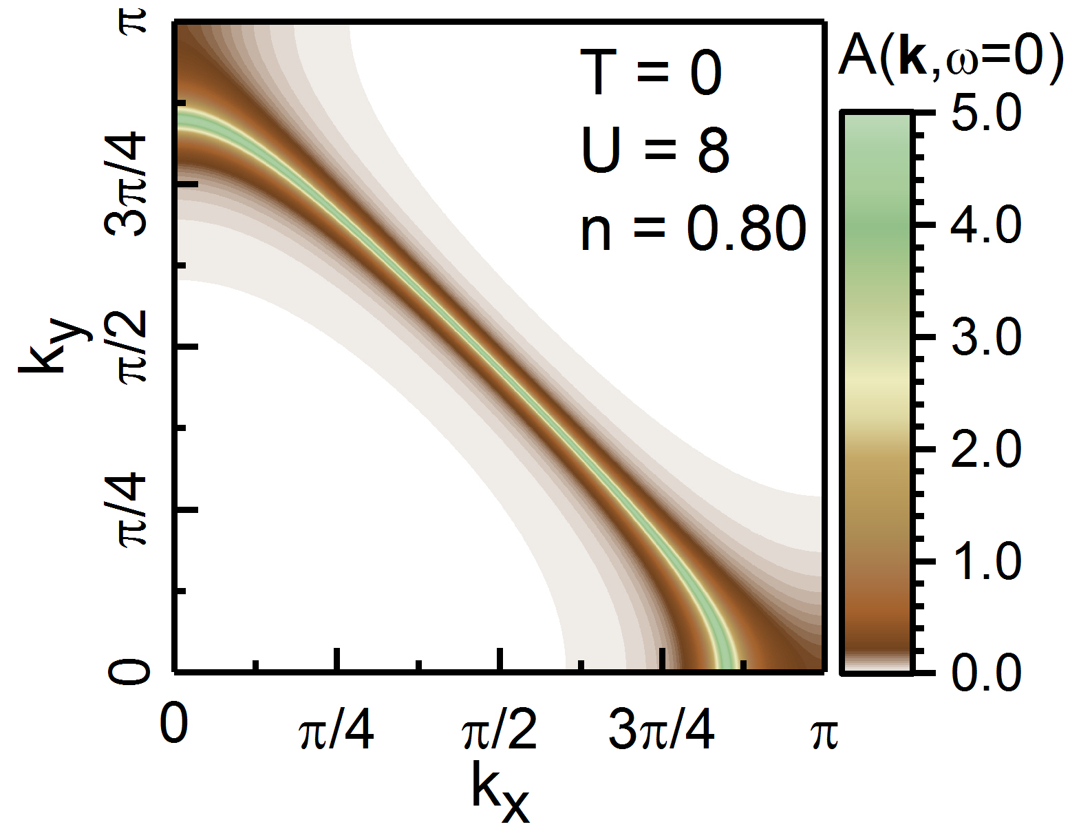
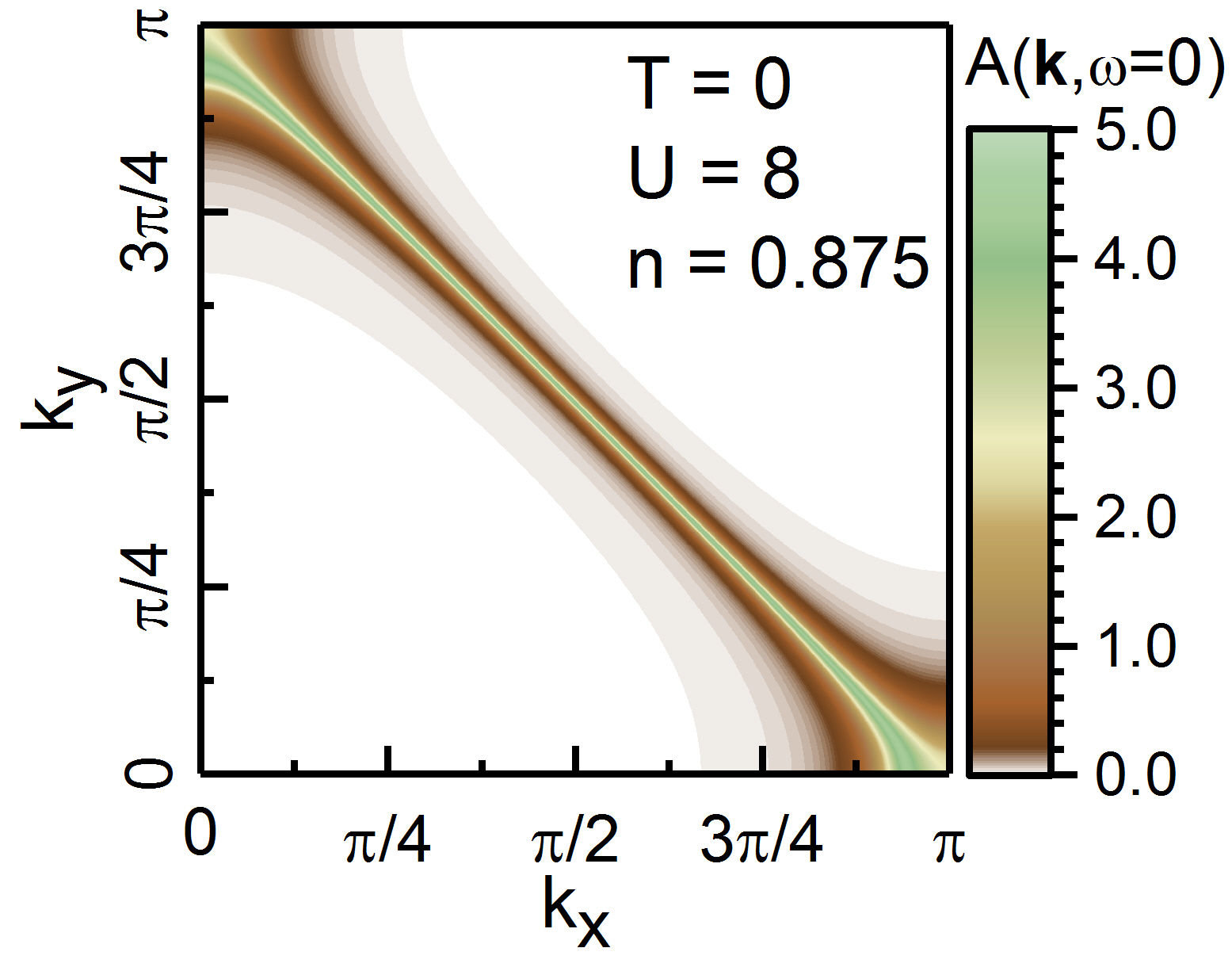
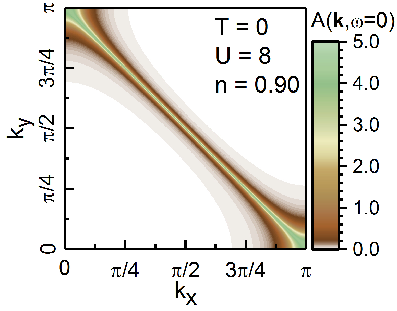
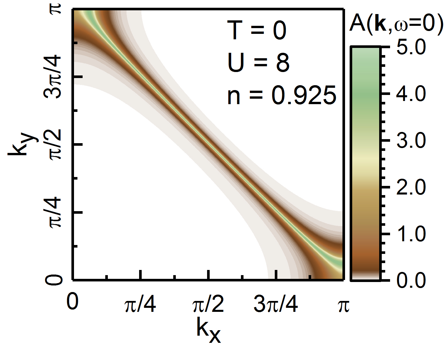
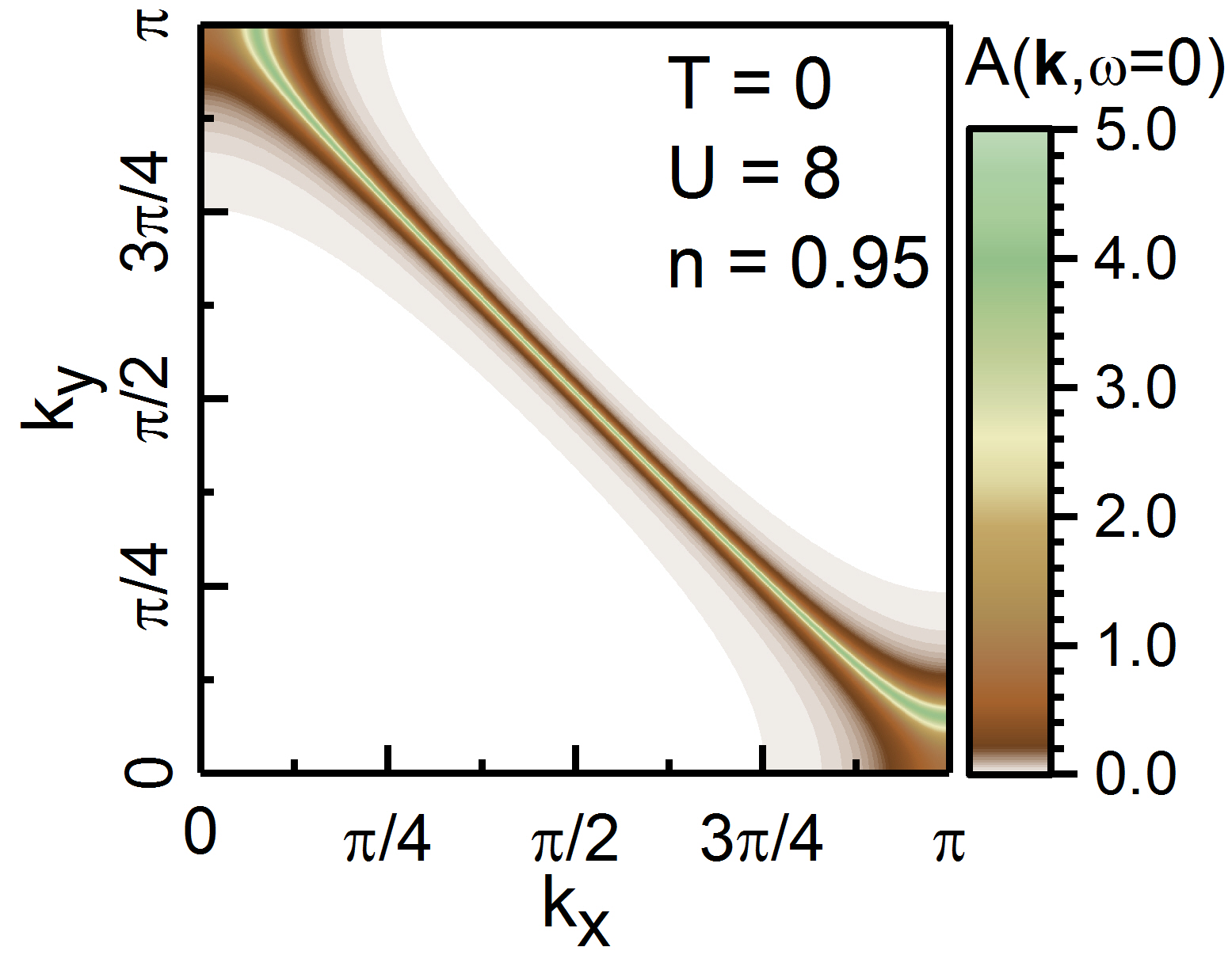
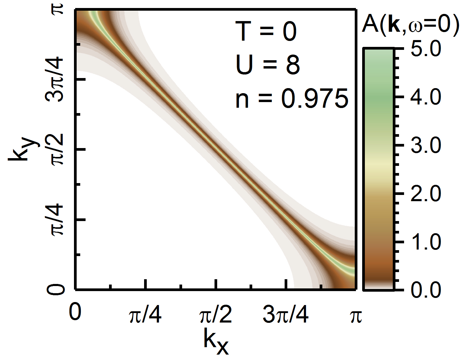
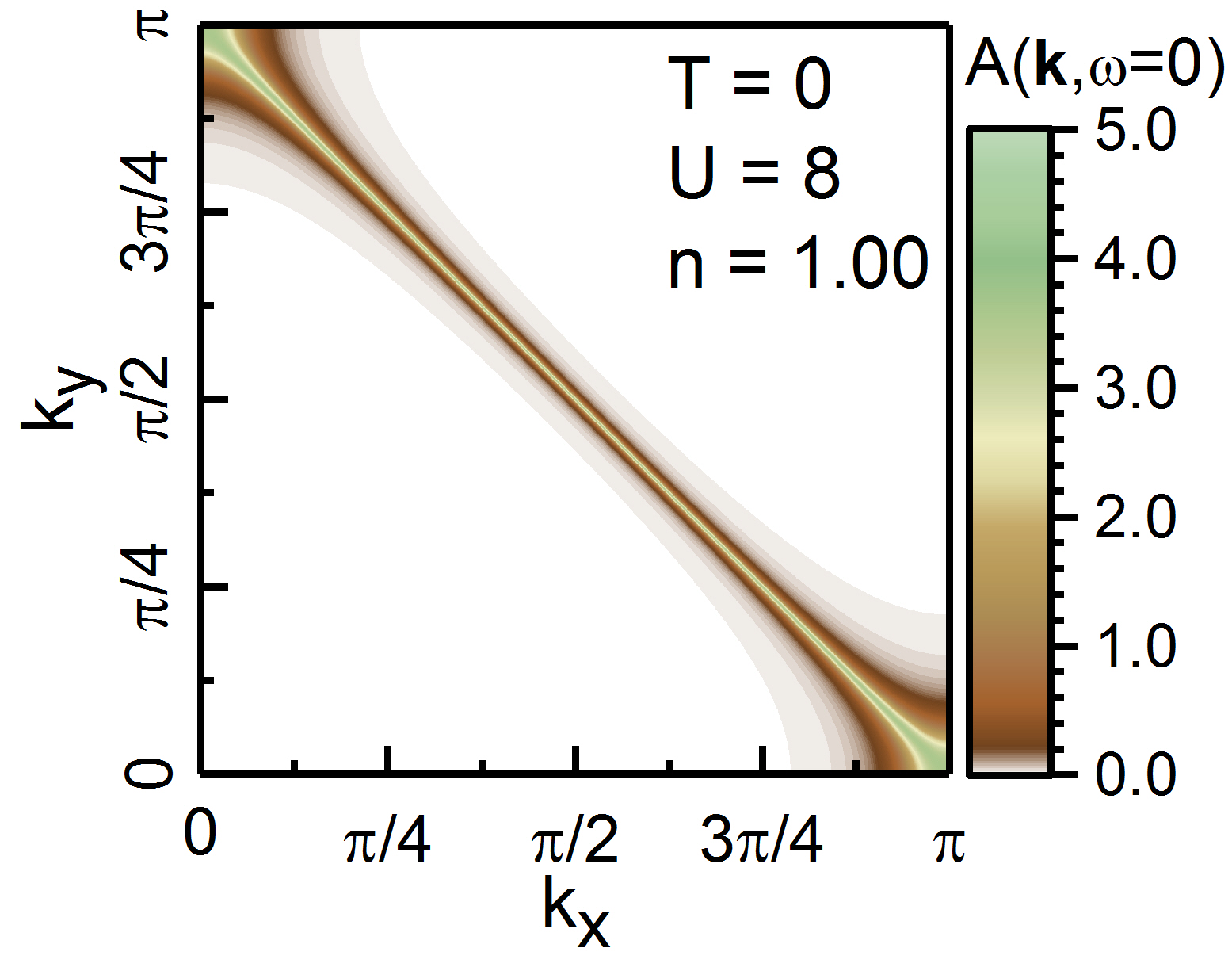
Figure 2: Fermi surface in the top-right quadrant of the first Brillouin zone read out through the maxima of $A\left(\mathbf{k},\omega=0\right)$ for various values of the doping at $T=0$ and $U=8$.

In order to better explore the different features of the energy bands and of the electronic weights, taking fully into account also the actual shape/curvature of the energy bands, between the two values of $U$, the density of states $N\left(\omega\right)$ for $T=0$ and $U=4$ (bottom row, left) and $U=8$ (bottom row, right) has also been reported in Fig. 1. The legend clearly reports the relationship between the different colors and the different values of the doping analyzed. Again, for the smaller value of $U$, $U=4$, the behavior is clearly monotonous and the vHs is clearly the higher peak at all dopings and reach the chemical potential only once at half filling following the evolution of the central band. The increase of weight in the other two bands, together with their going flat close to half filling, is now clearly visible in terms of well defined peak structures surrounding the main central peak. The indications of an unexpected and unconventional behavior coming from the energy bands at the higher value of $U$, $U=8$, is completely confirmed by the evolution of the density of states, which can also help us to better understand which is the emergent behavior. First, it is now evident that the vHs crossing happens twice: once at half filling as required by the Luttinger theorem, but also at a lower filling ($n=n_{\mathrm{vHs}}\cong 0.895$) signaling the establishment of quite strong correlations modifying the shape and the weights of the bands well beyond the weak-intermediate coupling limit well represented by the $U=4$ results. Moreover, the central peak is not anymore the highest one (at sufficiently low dopings): the two facts together can be interpreted as the precursors of the emergence of a pseudogap in the system in the region of doping close to half filling. The peaks of the other two bands get evidently higher and higher on decreasing the doping signaling the clear tendency towards the opening of the Mott-Hubbard gap. This latter was always somehow there between the two other bands, but the central band was filling it in for lower values of $U$. This mechanism will lead to a finite value of $U$ for the metal-insulator transition (MIT), that seems already close for $U=8$.

In Fig. 2, we report the doping evolution of the Fermi surface in the top-right quadrant of the first Brillouin zone read out through the maxima of $A\left(\mathbf{k},\omega=0\right)$ at $T=0$ and $U=8$. It is now clear that the Fermi surface changes concavity not at half filling as for $U=4$, according to the conventional weak-intermediate coupling scenario leading to a Fermi-like liquid abiding the Luttinger theorem, but at $n\cong 0.895$ leading to a clear violation of the Luttinger sum rule. This can be explained only taking into account that, in particular in the strong coupling regime, the new quasi-particles establishing in the system, and replacing the original electrons, are composite operators not satisfying canonical commutation relations and, accordingly, whose Green’s function is not bound to obey the Luttinger theorem.

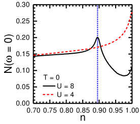
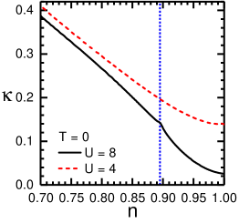
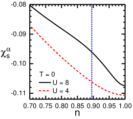
Figure 3: Density of states at the chemical potential $N\left(\omega=0\right)$ (top row, left), chemical potential $\mu$ (top row, right), compressibility $\kappa$ (bottom row, left) and nearest-neighbor spin-spin correlation function $\chi_{s}^{\alpha}$ (bottom row, right) as functions of the filling $n$ for $T=0$ and $U=4$ (red dashed line) and $U=8$ (black solid line). In all panels, the dotted blue line marks the filling at which $N\left(\omega=0\right)$ has a maximum.

Finally, in Fig. 3, we report the density of states at the chemical potential $N\left(\omega=0\right)$ (top row, left), the chemical potential $\mu$ (top row, right), the compressibility $\kappa=\frac{1}{n^{2}}\frac{\partial n}{\partial\mu}$ (bottom row, left) and the nearest-neighbor spin-spin correlation function $\chi_{s}^{\alpha}$ (bottom row, right) as functions of the filling $n$ for $T=0$ and $U=4$ (red dashed line) and $U=8$ (black solid line). In all panels, the dotted blue line marks the filling at which $N\left(\omega=0\right)$ has a maximum ($n=n_{\mathrm{vHs}}$). Looking at the doping evolution of the density of states at the chemical potential $N\left(\omega=0\right)$, it is now clear the fundamental difference of behavior between the solution at $U=4$ and at $U=8$. The former shows the typical behavior of a metal, the latter is on the verge of a MIT that is approached in a very unusual way: the vHs is efficiently crossed, with the related enhancement of the density of states, for a value of the filling smaller than $n=1$, namely $n=n_{\mathrm{vHs}}$. This can be clearly seen also in the chemical potential $\mu$ where the sudden change of slope at the same value of filling is more than evident as well as the clear tendency to reach a $\mu^{-}$ value, as it would happen at the MIT, rather than $\frac{U}{2}$. Even more, the compressibility $\kappa$ reports a clear kink at the same value of filling and a sudden reduction for smaller values of the doping, clearly signaling the upcoming emergence of an instability driven by the proximity to the MIT. As a matter of fact, it is the whole region of doping between $n=n_{\mathrm{vHs}}$ and half filling to exhibit clear fingerprints of strong correlations. In fact, the nearest-neighbor spin-spin correlations, captured by $\chi_{s}^{\alpha}$, show a net increase of intensity in that entire region of doping, also denouncing the origin of such behavior. The antiferromagnetic correlations, although still short range, appear to be strong enough, in the proximity of an incipient MIT, to dramatically modify the nature of the elementary excitations emerging in the system leading to the necessity of a description in terms of composite operators not necessarily obeying canonical commutation relations, whose treatment definitely requires an operatorial approach.

4 Conclusions

We have studied the single-particle properties of the 2D Hubbard model using the Composite Operator Method within a novel three-pole approximation whose operatorial basis includes, together with the usual Hubbard operator, a third field describing the electronic transitions dressed by the nearest-neighbor spin fluctuations. These latter have proved to play a crucial role in the unconventional behavior of the energy bands, the density of states and the Fermi surface of the system in the strong coupling regime ($U\geq 8$). In particular, so strong, although still short range, spin-spin correlations lead to the violation of the Luttinger sum rule that can be seen as a precursor of a pseudogap regime in proximity of an incipient MIT. The analysis of the doping evolution of the density of states at the chemical potential, of the chemical potential itself, of the compressibility and of the nearest-neighbor spin-spin correlation function provides further evidence that this scenario seems to be the one realized in the system. These findings also prove the necessity of a description of so strongly correlated systems in terms of composite operators, not necessarily obeying canonical commutation relations, within an operatorial approach.

References

- [1] J. Hubbard, Proc. Roy. Soc. A 276 (1963) 238.
- [2] J. Hubbard, Proc. Roy. Soc. A 277 (1964) 237.
- [3] J. Hubbard, Proc. Roy. Soc. A 281 (1964) 401.
- [4] K. A. Chao, J. Spałek, A. M. Oleś, J. Phys. C. 10 (1977) L271.
- [5] K. A. Chao, J. Spałek, A. M. Oleś, Phys. Rev. B 18 (1978) 3453.
- [6] V. J. Emery, Phys. Rev. Lett. 58 (1987) 2794.
- [7] V. J. Emery, G. Reiter, Phys. Rev. B 38 (1988) 4547.
- [8] V. J. Emery, S. A. Kivelson, Physica C 235 (1994) 189.
- [9] A. Avella, F. Mancini, F. P. Mancini, E. Plekhanov, Eur. Phys. J. B 86 (2013) 1.
- [10] F. Mancini, A. Avella, Adv. Phys. 53 (2004) 537.
- [11] A. Avella, F. Mancini, The composite operator method (com), in: A. Avella, F. Mancini (Eds.), Strongly Correlated Systems: Theoretical Methods, Vol. 171 of Springer Series in Solid-State Sciences, Springer Berlin Heidelberg, 2012, p. 103.
- [12] A. Avella, Eur. Phys. J. B 87 (2014) 45.
- [13] T. Timusk, B. Statt, Reports on Progress in Physics 62 (1999) 61.
- [14] A. Avella, Advances in Condensed Matter Physics 2014 (2014) 515698.
- [15] N. Bulut, D. J. Scalapino, S. R. White, Phys. Rev. B 50 (1994) 7215(R).
- [16] M. V. Sadovskii, I. A. Nekrasov, E. Z. Kuchinskii, T. Pruschke, V. I. Anisimov, Phys. Rev. B 72 (2005) 155105.
- [17] A. Avella, F. Mancini, Phys. Rev. B 75 (2007) 134518.