Abstract

We investigate the strength of the electroweak phase transition (EWPT) within the CP-violating 2-Higgs-Doublet Model (C2HDM). The 2HDM is a simple and well-studied model, which can feature CP violation at tree level in its extended scalar sector. This makes it, in contrast to the Standard Model (SM), a promising candidate for explaining the baryon asymmetry of the universe through electroweak baryogenesis. We apply a renormalisation scheme which allows efficient scans of the C2HDM parameter space by using the loop-corrected masses and mixing matrix as input parameters. This procedure enables us to investigate the possibility of a strong first order EWPT required for baryogenesis and study its phenomenological implications for the LHC. Like in the CP-conserving (real) 2HDM (R2HDM) we find that a strong EWPT favours mass gaps between the non-SM-like Higgs bosons. These lead to prominent final states comprised of gauge+Higgs bosons or pairs of Higgs bosons. In contrast to the R2HDM, the CP-mixing of the C2HDM also favours approximately mass degenerate spectra with dominant decays into SM particles. The requirement of a strong EWPT further allows us to distinguish the C2HDM from the R2HDM using the signal strengths of the SM-like Higgs boson. We additionally find that a strong EWPT requires an enhancement of the SM-like trilinear Higgs coupling at next-to-leading order (NLO) by up to a factor of 2.4 compared to the NLO SM coupling, establishing another link between cosmology and collider phenomenology. We provide several C2HDM benchmark scenarios compatible with a strong EWPT and all experimental and theoretical constraints. We include the dominant branching ratios of the non-SM-like Higgs bosons as well as the Higgs pair production cross section of the SM-like Higgs boson for every benchmark point. The pair production cross sections can be substantially enhanced compared to the SM and could be observable at the high-luminosity LHC, allowing access to the trilinear Higgs couplings.

1 Introduction

The discovery of the Higgs boson by the LHC experiments ATLAS [1] and CMS [2] has marked a milestone for particle physics while, at the same time, leaving many open questions. Despite the Standard Model (SM) nature of the Higgs boson [3, 4, 5, 6] new physics (NP) beyond the SM is called for in order to solve the puzzles within the standard theory. The observed baryon asymmetry of the Universe (BAU) [7] is one example that requires NP extensions. It can be generated dynamically in the early Universe during a first order electroweak phase transition (EWPT) through the mechanism of electroweak baryogenesis (EWBG) [8, 9, 10, 11, 12, 13, 14, 15, 16] provided that all three Sakharov conditions [17] are fulfilled. These are baryon number violation, C and CP violation and departure from the thermal equilibrium. A strong first order phase transition (PT) [14, 16] proceeds through bubble nucleation and can generate a net baryon number near the bubble wall. Diffusion through the bubble preserves this asymmetry for the later evolution of the universe by suppressing the sphaleron transitions in the false vacuum [18, 19]. A first order EWPT takes places when bubbles of the broken phase nucleate in the surrounding plasma of the symmetric phase. The bubble walls interact with the various fermion species in the plasma. If there is CP violation in the bubble wall or some CP violation in the hot i.e. the symmetric phase that is disturbed by the wall, particles with opposite chirality interact differently with the wall and CP and C asymmetries in particle number densities can be generated in front of the bubble wall. These asymmetries diffuse into the hot plasma ahead of the bubble wall biasing baryon number violating electroweak (EW) sphaleron transitions to generate a baryon asymmetry. The latter is transferred through the expanding wall into the broken phase. The rate of sphaleron transitions is strongly suppressed in this phase such that a washout of the baryons generated before is avoided. The required departure from thermodynamic equilibrium is guaranteed by the passage of the bubble walls that rapidly expand through the cosmological plasma. Additionally, gravitational waves produced by a strong first order EWPT [20] are potentially observable by the future space-based gravitational wave interferometer eLISA [21]. The interplay between gravitational waves and a strong first order PT and/or collider phenomenology has recently been studied in [22, 23, 24, 25, 26, 27, 28, 29, 30, 31, 32, 33, 34, 35, 36, 37, 38, 39, 40].

In the SM in principle all three Sakharov conditions could be realized. However, the EWPT is not of strong first order [41], since this would require a SM Higgs boson mass of around 70-80 GeV [42]. Additionally, the CP violation of the SM arising from the Cabibbo-Kobayashi-Maskawa (CKM) matrix is too small [16, 43, 44, 45]. Extensions beyond the SM provide additional sources of CP violation as well as further scalar states triggering a first order EWPT also for a SM-like Higgs boson with a mass of 125 GeV. This is the case for the 2-Higgs Doublet Model (2HDM) [46, 47] which belongs to the simplest NP extensions that are compatible with present experimental constraints. Previous studies have shown that 2HDMs provide a good framework for successful baryogenesis, both in the CP-conserving [48, 49, 50, 51, 52] and in the CP-violating case [53, 54, 55, 56, 57, 58, 29, 59]. 2HDMs feature five physical Higgs bosons, and the tree-level 2HDM Higgs sector provides sources for explicit CP violation. Allowing for CP violation, there could in principle be a complex phase between the vacuum expectation values (VEVs) of the two Higgs doublets. This phase can, however, always be removed by a change of basis [60] so that without loss of generality it can be set to zero. This may not be the case any more at finite temperature. CP violation might be generated spontaneously only in the bubble wall around the critical temperature [54] and provide a source for the generation of the matter-antimatter asymmetry through EWBG. The CP-violating phase which at zero temperature is just another parameter of the theory, during EWPT becomes a spatially varying field, and its value depends on the position relative to the bubble walls. In order to study the effect of CP violation on the generation of the baryon asymmetry the detailed form of the spatially varying field has to be determined.

CP-violating Higgs sectors are strongly constrained by the electric dipole moments (EDMs). The strongest constraint [61] is imposed by the limit on the electron EDM provided by the ACME collaboration [62]. The possibility of spontaneous CP violation generated at the EWPT which vanishes at zero temperature may provide an attractive scenario to lift the possible tension between the restrictions imposed by the EDMs and the requirement of a substantial amount of CP violation by the EWBG.

In [51] we investigated the implications of a strong first order PT in the CP-conserving or real 2HDM (R2HDM) on the LHC Higgs phenomenology. We found a strong interplay between the requirement of successful baryogenesis and LHC Higgs phenomenology. In this work, we extend our analysis to the CP-violating 2HDM (C2HDM). The computation of the equation of motion for the CP-violating phase between the two Higgs doublets and the computation of the actual baryon-antibaryon asymmetry generated through EWBG within the framework of the C2HDM is beyond the scope of this paper. We focus instead on the interplay between the requirement of a strong first order phase transition and LHC phenomenology in the presence of explicit CP violation in the tree-level 2HDM Higgs sector. We investigate the possible spontaneous generation of a CP-violating phase at the EWPT. We furthermore analyse in detail the effect of higher order corrections on the trilinear Higgs self-couplings extracted from the one-loop corrected effective potential. We discuss the impact of the requirement of a strong phase transition on their size and the resulting implications for LHC phenomenology, namely Higgs pair production. We present several benchmark scenarios, emphasizing the specific features of C2HDM parameter points compatible with all constraints and a strong phase transition.

For the purpose of this paper we compute the one-loop corrected effective potential at finite temperature [69, 71, 70] including daisy resummations for the bosonic masses [72]. For the numerical analysis the parameter space of the C2HDM is scanned and tested for compatibility of the model with the theoretical and experimental constraints. Subsequently, the implication of a strong first order PT on the surviving parameter sets is determined and interpreted with respect to collider phenomenology. The former necessitates the minimisation of the loop-corrected Higgs potential at increasing temperature in order to find the vacuum expectation value $v_{c}$ at the critical temperature $T_{c}$, which is defined as the temperature where two degenerate global minima exist. A value of $v_{c}/T_{c}$ larger than one is indicative of a strong first order PT [11, 73]. In order to be able to perform an efficient scan, like in [51], we renormalise the loop-corrected potential in such a way that not only the VEV and all physical Higgs boson masses, but also all mixing matrix elements remain at their tree-level values. In our analysis, we will focus on the C2HDM with type I and type II couplings of the Higgs doublets to the fermions. We will discard parameter points inducing a 2-stage PT [77, 78]. Our analysis reveals a strong link between the demand for a strong first order PT and testable implications at the collider experiments.

The outline of the paper is as follows: In section 2 we set our notation and present the loop-corrected effective potential of the C2HDM at finite temperature. Our renormalisation procedure is described in section 3. Section 4 is dedicated to the description of the numerical analysis. It includes the outline of the minimisation procedure of the effective potential and the details of the scan in the C2HDM parameter space as well as of the applied theoretical and experimental constraints. Sections 5-10 contain our results. In Section 6 we analyse the type I C2HDM with the lightest Higgs boson being the SM-like Higgs state. We first investigate the spontaneous generation of a CP-violating phase and its relation to explicit CP violation in the tree-level potential. We then present the parameter regions compatible with the applied constraints and a strong first order PT and analyse the implications for collider phenomenology. In Section 7 we discuss in detail the role of the trilinear Higgs self-couplings in the EWPT, the impact of the next-to-leading order (NLO) corrections derived from the effective potential and the implications of the requirement of a strong phase transition on the Higgs self-couplings and their corrections. In Section 8 we briefly summarise the results for the type I C2HDM with the next-to-lightest Higgs boson representing the SM-like Higgs scalar. Sections 9 and 10 are dedicated to the type II C2HDM with the lightest Higgs boson being SM-like, and we present our results in analogy to the type I case. Section 11 contains our conclusions.

2 The effective potential in the C2HDM

In this section we provide the loop-corrected effective potential at finite temperature for the CP-violating 2HDM. We start by setting our notation.

2.1 The CP-violating 2-Higgs-Doublet Model

The tree-level potential of the C2HDM for the two $SU(2)_{L}$ scalar doublets

$$\Phi_{1}=\left(\begin{array}[]{c}\phi_{1}^{+}\\ \phi_{1}^{0}\end{array}\right)\quad\mbox{and}\quad\Phi_{1}=\left(\begin{array}[]{c}\phi_{2}^{+}\\ \phi_{2}^{0}\end{array}\right)\;,$$ (5)

reads

$$\begin{split}V_{\text{tree}}&=m_{11}^{2}\Phi_{1}^{\dagger}\Phi_{1}+m_{22}^{2}\Phi_{2}^{\dagger}\Phi_{2}-\left[m_{12}^{2}\Phi_{1}^{\dagger}\Phi_{2}+\mathrm{h.c.}\right]+\frac{1}{2}\lambda_{1}(\Phi_{1}^{\dagger}\Phi_{1})^{2}+\frac{1}{2}\lambda_{2}(\Phi_{2}^{\dagger}\Phi_{2})^{2}\\ &\quad+\lambda_{3}(\Phi_{1}^{\dagger}\Phi_{1})(\Phi_{2}^{\dagger}\Phi_{2})+\lambda_{4}(\Phi_{1}^{\dagger}\Phi_{2})(\Phi_{2}^{\dagger}\Phi_{1})+\left[\frac{1}{2}\lambda_{5}(\Phi_{1}^{\dagger}\Phi_{2})^{2}+\mathrm{h.c.}\right]\;.\end{split}$$ (6)

It incorporates a softly broken $\mathbb{Z}_{2}$ symmetry, under which the doublets transform as $\Phi_{1}\rightarrow\Phi_{1},\ \Phi_{2}\rightarrow-\Phi_{2}$. This ensures the absence of tree-level Flavor Changing Neutral Currents (FCNC). The hermiticity of the potential $V_{\text{tree}}$ forces all parameters to be real apart from the soft $\mathbb{Z}_{2}$ breaking mass parameter $m_{12}^{2}$ and the quartic coupling $\lambda_{5}$. For $\mbox{arg}(m_{12}^{2})=\mbox{arg}(\lambda_{5})$ the complex phases of these two parameters can be absorbed by a basis transformation. If furthermore the VEVs of the two doublets are assumed to be real, we are in the real or CP-conserving 2HDM. Otherwise, we are in the C2HDM, for which we will adopt the conventions of [79] in the following.

After EW symmetry breaking the two Higgs doublets acquire VEVs $\bar{\omega}_{i}\in\mathbb{R}$, about which the Higgs fields can be expanded in terms of the charged CP-even and CP-odd fields $\rho_{i}$ and $\eta_{i}$, and the neutral CP-even and CP-odd fields $\zeta_{i}$ and $\psi_{i}$, $i=1,2$. In the general 2HDM, there are three different types of minima, given by the normal EW-breaking one, a CP-breaking minimum, and a charge-breaking (CB) vacuum. In Refs. [80, 81, 82] it has been shown that at tree level minima that break different symmetries cannot coexist. If a normal minimum exists, all CP or CB stationary points are proven to be saddle points. These statements may not be true any more at higher orders, as recent studies have shown for the Inert 2HDM at one-loop level in the effective potential approach [83]. Consequently, we allow for the possibility of a CP-breaking vacuum as well as a charge-breaking one. Through the VEVs $\bar{\omega}_{\text{CP}}$ and $\bar{\omega}_{\text{CB}}$ we include the possibility of generating at one-loop and/or non-zero temperature a global minimum that is CP-violating and/or charge breaking. As a charge-breaking VEV breaks electrical charge conservation inducing a massive photon, this unphysical configuration of the vacuum will not further be discussed in the numerical analysis. Denoting the VEVs of the normal vacuum by $\bar{\omega}_{1,2}$ and the CP- and charge-breaking VEVs by $\bar{\omega}_{\text{CP}}$ and $\bar{\omega}_{\text{CB}}$, respectively, the expansion of the two Higgs doublets about the VEVs is given by

$$\Phi_{1} =\frac{1}{\sqrt{2}}\begin{pmatrix}\rho_{1}+\mathrm{i}\eta_{1}\\ \bar{\omega}_{1}+\zeta_{1}+\mathrm{i}\psi_{1}\end{pmatrix}$$ (7)

$$\Phi_{2} =\frac{1}{\sqrt{2}}\begin{pmatrix}\bar{\omega}_{\text{CB}}+\rho_{2}+\mathrm{i}\eta_{2}\\ \bar{\omega}_{2}+\mathrm{i}\bar{\omega}_{\text{CP}}+\zeta_{2}+\mathrm{i}\psi_{2}\end{pmatrix}\,,$$ (8)

where, without loss of generality, the complex part of the VEVs and the charge-breaking VEV have been rotated to the second doublet exclusively. The VEVs of our present vacuum at zero temperature are denoted as

$$v_{i}\equiv\bar{\omega}_{i}|_{T=0}\;,\quad i=\mbox{1,\,2,\,CP,\,CB}\;,$$ (9)

with

$$v_{\text{CP}}=v_{\text{CB}}=0\;.$$ (10)

The VEVs of the normal vacuum, $v_{1,2}$, are related to the SM VEV $v\approx 246$ GeV by

$$v_{1}^{2}+v_{2}^{2}\equiv v^{2}\;.$$ (11)

The angle $\beta$ defines the ratio of $v_{1}$ and $v_{2}$,

$$\tan\beta=\frac{v_{2}}{v_{1}}\;,$$ (12)

so that

$$v_{1}=v\cos\beta\qquad\mbox{and}\qquad v_{2}=v\sin\beta\ .$$ (13)

The minimum conditions of the potential Eq. (6),

$$\left.\frac{\partial V_{\text{tree}}}{\partial\Phi_{i}^{\dagger}}\right|_{\Phi_{j}=\langle\Phi_{j}\rangle} \overset{!}{=}0\qquad i,j\in\{1,2\}\;,$$ (14)

where the brackets denote the Higgs field values in the minimum, i.e. $\langle\Phi_{i}\rangle=(0,v_{i}/\sqrt{2})$ at $T=0$, result in

$$m_{11}^{2} =\mbox{Re}(m_{12}^{2})\frac{v_{2}}{v_{1}}-\frac{v_{1}^{2}}{2}\lambda_{1}-\frac{v_{2}^{2}}{2}\lambda_{345}$$ (15a)

$$m_{22}^{2} =\mbox{Re}(m_{12}^{2})\frac{v_{1}}{v_{2}}-\frac{v_{2}^{2}}{2}\lambda_{2}-\frac{v_{1}^{2}}{2}\lambda_{345}$$ (15b)

$$2\,\mbox{Im}(m_{12}^{2}) =v_{1}v_{2}\,\mbox{Im}(\lambda_{5})\;,$$ (15c)

where we have introduced the abbreviation

$$\lambda_{345}\equiv\lambda_{3}+\lambda_{4}+\mbox{Re}(\lambda_{5})\;.$$ (16)

Equations (15a) and (15b) can be used to trade the parameters $m_{11}^{2}$ and $m_{22}^{2}$ for $v_{1}$ and $v_{2}$, while Eq. (15c) leads to a relation between the two sources of CP violation in the scalar potential so that one of the ten parameters of the C2HDM is fixed. Introducing

$$\zeta_{3}=-\psi_{1}\sin\beta+\psi_{2}\cos\beta\;,$$ (17)

the neutral mass eigenstates $H_{i}$ ($i=1,2,3$) are obtained from the C2HDM basis $\zeta_{1}$, $\zeta_{2}$ and $\zeta_{3}$ through the rotation

$$\left(\begin{array}[]{c}H_{1}\\ H_{2}\\ H_{3}\end{array}\right)=R\left(\begin{array}[]{c}\zeta_{1}\\ \zeta_{2}\\ \zeta_{3}\end{array}\right)\;.$$ (24)

The corresponding Higgs masses are obtained from the mass matrix

$$({\cal M}^{2})_{ij}=\left\langle\frac{\partial^{2}V}{\partial\zeta_{i}\partial\zeta_{j}}\right\rangle\;,$$ (25)

through the diagonalisation with the matrix $R$,

$$R{\cal M}^{2}R^{T}=\mbox{diag}(m_{H_{1}}^{2},m_{H_{2}}^{2},m_{H_{3}}^{2})\;.$$ (26)

The Higgs bosons are ordered by ascending mass as $m_{H_{1}}\leq m_{H_{2}}\leq m_{H_{3}}$. With the abbreviations $s_{i}\equiv\sin\alpha_{i}$ and $c_{i}\equiv\cos\alpha_{i}$, where

$$-\frac{\pi}{2}\leq\alpha_{i}<\frac{\pi}{2}\;,$$ (27)

the mixing matrix $R$ can be parametrised as

$$R=\left(\begin{array}[]{ccc}c_{1}c_{2}&s_{1}c_{2}&s_{2}\\ -(c_{1}s_{2}s_{3}+s_{1}c_{3})&c_{1}c_{3}-s_{1}s_{2}s_{3}&c_{2}s_{3}\\ -c_{1}s_{2}c_{3}+s_{1}s_{3}&-(c_{1}s_{3}+s_{1}s_{2}c_{3})&c_{2}c_{3}\end{array}\right)\;.$$ (31)

Exploiting the minimum conditions of the potential at zero temperature, we use the following set of 9 independent parameters of the C2HDM [84],

$$v\;,\quad t_{\beta}\;,\quad\alpha_{1,2,3}\;,\quad m_{H_{i}}\;,\quad m_{H_{j}}\;,\quad m_{H^{\pm}}\quad\mbox{and}\quad\mbox{Re}(m_{12}^{2})\;.$$ (32)

The $m_{H_{i}}$ and $m_{H_{j}}$ denote any two among the three neutral Higgs boson masses, and the mass of the third Higgs boson is obtained from the other parameters [84]. For the analytic relations between the above parameter set and the coupling parameters $\lambda_{i}$ of the 2HDM Higgs potential, see [79].

The limit of the CP-conserving 2HDM is obtained for $\alpha_{2}=\alpha_{3}=0$ and $\alpha_{1}=\alpha+\pi/2$ [85]. The mass matrix Eq. (25) becomes block diagonal in this case leading to the pure pseudoscalar $A$, which is identified with $H_{3}$, and the CP-even mass eigenstates $h$ and $H$, which are obtained from the gauge eigenstates $\zeta_{1,2}$ through the rotation with the angle $\alpha$,

$$\left(\begin{array}[]{c}H\\ h\end{array}\right)=\left(\begin{array}[]{cc}c_{\alpha}&s_{\alpha}\\ -s_{\alpha}&c_{\alpha}\end{array}\right)\left(\begin{array}[]{c}\zeta_{1}\\ \zeta_{2}\end{array}\right)\;.$$ (39)

The imposed $\mathbb{Z}_{2}$ symmetry ensures that each of the up-type quarks, down-type quarks and charged leptons can only couple to one of the Higgs doublets so that FCNCs at tree level are avoided. Table 1 lists the possible different 2HDM types given by type I, type II, lepton-specific and flipped.

	Type I	Type II	Lepton-Specific	Flipped
Up-type quarks	$\Phi_{2}$	$\Phi_{2}$	$\Phi_{2}$	$\Phi_{2}$
Down-type quarks	$\Phi_{2}$	$\Phi_{1}$	$\Phi_{2}$	$\Phi_{1}$
Leptons	$\Phi_{2}$	$\Phi_{1}$	$\Phi_{1}$	$\Phi_{2}$

Table 1: Classification of the Yukawa sector in the 2HDM according to the couplings of the fermions to the Higgs doublets.

For the exact form of the C2HDM Higgs couplings to the SM particles in terms of the input parameters, we refer to Refs. [86, 87, 88]. In this work we focus on C2HDMs of type I and type II.

2.2 One-loop effective potential at finite temperature

The form of the one-loop effective potential at finite temperature for the C2HDM case does not change with respect to the one introduced for the CP-conserving 2HDM in Ref. [51]. For convenience of the reader, we briefly repeat the main ingredients, also in order to set our notation.

The one-loop contribution $V_{1}$ to the effective potential consists of the Coleman-Weinberg (CW) contribution $V_{\text{CW}}$ [69] already present at zero temperature, and the contribution $V_{T}$ for the thermal corrections at finite temperature $T$. The one-loop corrected effective potential reads

$$V=V_{\text{tree}}+V_{1}\equiv V_{\text{tree}}+V_{\text{CW}}+V_{T}\,,$$ (40)

with the tree-level potential given in Eq. (6) after replacing the doublets $\Phi_{1,2}$ with their classical constant field configuration

$$\Phi_{1}^{c}=\left(\begin{array}[]{c}0\\ \frac{\omega_{1}}{\sqrt{2}}\end{array}\right)\quad\mbox{and}\quad\Phi_{2}^{c}=\left(\begin{array}[]{c}\frac{\omega_{\text{CB}}}{\sqrt{2}}\\ \frac{\omega_{2}+i\omega_{\text{CP}}}{\sqrt{2}}\end{array}\right)\;.$$ (45)

In the $\overline{\text{MS}}$ scheme the Coleman-Weinberg potential for a particle $i$ reads [71]

$$V_{\text{CW}}(\{\omega\})=\sum_{i}\frac{n_{i}}{64\pi^{2}}(-1)^{2s_{i}}\,m_{i}^{4}(\{\omega\})\,\left[\log\left(\frac{m_{i}^{2}(\{\omega\})}{\mu^{2}}\right)-c_{i}\right]\,.$$ (46)

The sum extends over the Higgs and Goldstone bosons, the massive gauge bosons, the longitudinal photon and the fermions $f$, with the exception of the neutrinos, which we assume to be massless, $i=h,H,A,H^{\pm},G^{0},G^{\pm},W^{\pm},Z,\gamma_{L},f$. Here, $m_{i}^{2}$ denotes the respective eigenvalue for the particle $i$ of the mass matrix squared expressed through the tree-level relations in terms of $\omega_{i}$ ($i=1,\,2,\,\mbox{CP},\,\mbox{CB}$). The sum also extends over the Goldstone bosons and the photon. Although in the Landau gauge applied here the Goldstone bosons are massless at $T=0$, they can become massive for field configurations different from the tree-level VEVs at $T=0$, which are required in the minimisation procedure. This is also the case for the photon, as we allow for non-physical vacuum configurations with a non-zero charge breaking VEV. Furthermore, the Goldstone bosons and the longitudinal photon can become massive due to the temperature corrections discussed below. Because of the Landau gauge we need not consider any ghost contributions. The spin of the particle is denoted by $s_{i}$ and the number of degrees of freedom by $n_{i}$. For the scalars $\Phi=H_{i},G^{0},H^{+},H^{-},G^{+},G^{-}$, the charged leptons $l^{+}$ and $l^{-}$, the quarks and antiquarks $q$ and $\bar{q}$, the longitudinal and transversal gauge bosons $V_{L}=Z_{L},W^{+}_{L},W^{-}_{L},\gamma_{L}$ and $V_{T}=Z_{T},W^{+}_{T},W^{-}_{T},\gamma_{T}$, they are

$$\begin{array}[]{llllllllll}n_{\Phi}&=&1\;,&\quad n_{l^{+}}&=&2\;,&\quad n_{l^{-}}&=&2\;,\\ n_{q}&=&6\;,&\quad n_{\bar{q}}&=&6\;,&\quad n_{V_{T}}&=&2\;,&\quad n_{V_{L}}=1\;.\end{array}$$ (49)

In the $\overline{\text{MS}}$ scheme employed here the constants $c_{i}$ read

$$c_{i}=\begin{cases}\frac{5}{6}\ ,&i=W^{\pm},Z,\gamma\\ \frac{3}{2}\ ,&\text{otherwise}\ .\end{cases}$$ (50)

The renormalisation scale $\mu$ is fixed to $\mu=v=246.22\ \text{GeV}$.

The thermal corrections $V_{T}$ comprise the daisy resummation [72] of the $n=0$ Matsubara modes of the longitudinal components of the gauge bosons $W_{L}^{+},W_{L}^{-},Z_{L},\gamma_{L}$ and the bosons $\Phi$, so that their masses receive Debye corrections at non-zero temperature. The potential $V_{T}$ can be cast into the form [70, 71]

$$V^{T}=\sum_{k}n_{k}\,\frac{T^{4}}{2\pi^{2}}\,J^{(k)}_{\pm}\;,$$ (51)

with $k=W_{L}^{+},W_{L}^{-},Z_{L},\gamma_{L},W_{T}^{+},W_{T}^{-},Z_{T},\gamma_{T},\Phi,l^{+},l^{-},q,\bar{q}$. Since the Goldstone bosons and the photon acquire a mass at finite temperature, they have to be included in the sum. Denoting the mass eigenvalue including the thermal corrections for the particle $k$ by $\overline{m}_{k}$, we have for $J_{\pm}^{(k)}$ (see e.g. [89])

$$J^{(k)}_{\pm}=\left\{\begin{array}[]{ll}J_{-}\left(\frac{m_{k}^{2}}{T^{2}}\right)-\frac{\pi}{6}(\overline{m}_{k}^{3}-m_{k}^{3})&k=W_{L}^{+},W_{L}^{-},Z_{L},\gamma_{L},\Phi\\ J_{-}\left(\frac{m_{k}^{2}}{T^{2}}\right)&k=W_{T}^{+},W_{T}^{-},Z_{T},\gamma_{T}\\ J_{+}\left(\frac{m_{k}^{2}}{T^{2}}\right)&k=l^{+},l^{-},q,\bar{q}\end{array}\right.$$ (55)

with the thermal integrals

$$J_{\pm}\left(\frac{m_{k}^{2}}{T^{2}}\right)=\mp\int_{0}^{\infty}\text{d}x\,x^{2}\log\left[1\pm e^{-\sqrt{x^{2}+m_{k}^{2}/T^{2}}}\right]\ ,$$ (56)

where $J_{+}$ ($J_{-}$) applies for $k$ being a fermion (boson). The masses $m_{i}$ depend implicitly on the temperature $T$, since for each $T$ we determine the VEVs, respectively the field configurations, $\bar{\omega}_{i}=\bar{\omega}_{i}(T)$, that minimise the loop-corrected potential $V$, Eq. (40). These field configurations enter the tree-level mass matrices. The $\overline{m}_{k}$ in addition depend explicitly on $T$ through the thermal corrections. With the definition of $J^{(k)}_{\pm}$ Eq. (55) we follow the ’Arnold-Espinosa’ approach of Ref. [90]. A different approach has been proposed in [91], to which we refer as ’Parwani’ method. Here the Debye corrections are included for all the bosonic thermal loop contributions and the Debye corrected masses are also used in the CW potential. Since the ’Parwani’ method admixes higher-order contributions, possibly leading to dangerous artifacts at one-loop level, we apply the ’Arnold-Espinosa’ method. For a discussion and comparison of the two methods, see also [56, 58].

The minimisation procedure requires the numerical evaluation of the integral Eq. (56) at each configuration in $\{\omega\}$ and $T$, which is very time consuming. The integrals $J_{\pm}$ are therefore approximated by a series in $x^{2}\equiv m^{2}/T^{2}$. For small $x^{2}$ we have [56]

$$\begin{split}J_{+,\text{s}}(x^{2},n)&=-\frac{7\pi^{4}}{360}+\frac{\pi^{2}}{24}x^{2}+\frac{1}{32}x^{4}\left(\log x^{2}-c_{+}\right)\\ &\quad-\pi^{2}x^{2}\sum_{l=2}^{n}\left(-\frac{1}{4\pi^{2}}x^{2}\right)^{l}\frac{(2l-3)!!\zeta(2l-1)}{(2l)!!(l+1)}\left(2^{2l-1}-1\right)\end{split}$$ (57)

$$\begin{split}J_{-,\text{s}}(x^{2},n)&=-\frac{\pi^{4}}{45}+\frac{\pi^{2}}{12}x^{2}-\frac{\pi}{6}\left(x^{2}\right)^{3/2}-\frac{1}{32}x^{4}\left(\log x^{2}-c_{-}\right)\\ &\quad+\pi^{2}x^{2}\sum_{l=2}^{n}\left(-\frac{1}{4\pi^{2}}x^{2}\right)^{l}\frac{(2l-3)!!\zeta(2l-1)}{(2l)!!(l+1)}\ ,\end{split}$$ (58)

with

$$c_{+}=3/2+2\log\pi-2\gamma_{E}\quad\mbox{and}\quad c_{-}=c_{+}+2\log 4\;,$$ (59)

where $\gamma_{E}$ denotes the Euler-Mascheroni constant, $\zeta(x)$ the Riemann $\zeta$-function and $(x)!!$ the double factorial. For large $x^{2}$ we use for both the fermions and the bosons [56]

$$J_{\pm,\text{l}}(x^{2},n)=-\exp\left(-\left(x^{2}\right)^{1/2}\right)\left(\frac{\pi}{2}\left(x^{2}\right)^{3/2}\right)^{1/2}\sum_{l=0}^{n}\frac{1}{2^{l}l!}\frac{\Gamma(5/2+l)}{\Gamma(5/2-l)}\left(x^{2}\right)^{-l/2}\ ,$$ (60)

with $\Gamma(x)$ denoting the Euler Gamma function. For the interpolation between the two approximations the point is determined where the derivatives of the low- and high-temperature expansions can be connected continuously. At this point a small finite shift to the small $x^{2}$ expansion is added such that also the two expansions themselves are connected continuously. Denoting the values of $x^{2}$ where the connection is performed, by $x^{2}_{+}$ and $x^{2}_{-}$ and the corresponding shifts by $\delta_{\pm}$ for the fermionic and bosonic contributions, respectively, they are given by

$$\begin{array}[]{lcllcl}x^{2}_{+}&=&2.2161\;,&\qquad\delta_{+}&=&-0.015603\;,\\ x^{2}_{-}&=&9.4692\;,&\qquad\delta_{-}&=&0.0063109\;.\end{array}$$ (63)

For small $x^{2}$ the exact result is well approximated by including terms of up to order $n=4$ in the expansion $J_{+,\text{s}}$ for fermions, for bosons this is the case for $n=3$ in $J_{-,\text{s}}$. For large $x^{2}$, the integral is well approximated by $n=3$ in both the fermion and the boson case, $J_{\pm,\text{l}}$. The deviation of the approximate results from the numerical evaluation of the integrals is less than two percent. The approximations Eqs. (57)-(60) are only valid for $m^{2}\geq 0$. For bosons this is not necessarily the case as the eigenvalues of the mass matrix of the neutral Higgs bosons can become negative for certain configurations $\{\omega\}$ and temperatures $T$ in the minimisation procedure. In this case the value of the integral $J_{-}$, Eq. (56), is set to the real part of its numerical evaluation which is the relevant contribution for the extraction of the global minimum [92]. In practice, the integral is evaluated numerically at several equidistant points in $m^{2}/T^{2}<0$, and in the minimisation procedure the result obtained from the linear interpolation between these points is used. This allows for a significant speed-up. We explicitly verified that the difference between the exact and the interpolated result is negligible for a sufficiently large range of $m^{2}/T^{2}$.

3 Renormalisation

The masses and mixing angles extracted from the loop-corrected potential differ from those extracted from the tree-level potential. In the tests for the compatibility of the model with the experimental constraints these corrections have to be taken into account. In order to ensure an efficient scan over the parameter space of the model in terms of the input parameters Eq. (32), it is more convenient to directly use the loop-corrected masses and angles as inputs. We therefore modify the $\overline{\text{MS}}$ renormalisation applied in the Coleman-Weinberg potential Eq. (46) and choose a renormalisation prescription by which we enforce the one-loop corrected masses and mixing matrix elements to be equal to the tree-level ones. This follows the approach chosen in our analysis of the CP-conserving 2HDM [51]. The counterterm potential $V_{\text{CT}}$, which is added to the one-loop effective potential Eq. (40),

$$\tilde{V}=V+V_{\text{CT}}=V_{\text{tree}}+V_{\text{CW}}+V_{T}+V_{\text{CT}}\;,$$ (64)

reads

$$V_{\text{CT}} = \frac{\delta m_{11}^{2}}{2}\omega_{1}^{2}+\frac{\delta m_{22}^{2}}{2}(\omega_{2}^{2}+\omega_{\text{CP}}^{2}+\omega_{\text{CB}}^{2})-\delta\mbox{Re}(m_{12}^{2})\,\omega_{1}\omega_{2}+\delta\mbox{Im}(m_{12}^{2})\,\omega_{1}\omega_{\text{CP}}+\frac{\delta\lambda_{1}}{8}\omega_{1}^{4}$$ (65)

$$+ \frac{\delta\lambda_{2}}{8}(\omega_{2}^{2}+\omega_{\text{CP}}^{2}+\omega_{\text{CB}}^{2})^{2}+\frac{\delta\lambda_{3}}{4}\omega_{1}^{2}\left(\omega_{2}^{2}+\omega_{\text{CP}}^{2}+\omega_{\text{CB}}^{2}\right)+\frac{\delta\lambda_{4}}{4}\omega_{1}^{2}\left(\omega_{2}^{2}+\omega_{\text{CP}}^{2}\right)$$

$$+ \frac{\delta\mbox{Re}(\lambda_{5})}{4}\omega_{1}^{2}\left(\omega_{2}^{2}-\omega_{\text{CP}}^{2}\right)-\frac{\delta\mbox{Im}(\lambda_{5})}{2}\omega_{1}^{2}\omega_{2}\omega_{\text{CP}}$$

$$+ \delta T_{1}\,\omega_{1}+\delta T_{2}\,\omega_{2}+\delta T_{\text{CP}}\,\omega_{\text{CP}}\;.$$

In the last line we explicitly included the tadpole counterterms $\delta T$ for the directions in field space in which we allow for the development of a vacuum. Since we check for the compatibility with the experimental constraints at $T=0$ we apply our renormalisation conditions at this temperature. They are given by ($i,j=1,...,8$)

$$\partial_{\phi_{i}}\left.V_{\text{CT}}(\phi)\right|_{\phi=\langle\phi^{c}\rangle_{T=0}} = -\partial_{\phi_{i}}\left.V_{\text{CW}}(\phi)\right|_{\phi=\langle\phi^{c}\rangle_{T=0}}$$ (66)

$$\partial_{\phi_{i}}\partial_{\phi_{j}}\left.V_{\text{CT}}(\phi)\right|_{\phi=\langle\phi^{c}\rangle_{T=0}} = -\partial_{\phi_{i}}\partial_{\phi_{j}}\left.V_{\text{CW}}(\phi)\right|_{\phi=\langle\phi^{c}\rangle_{T=0}}\;,$$ (67)

with

$$\phi_{i}\equiv\{\rho_{1},\eta_{1},\rho_{2},\eta_{2},\zeta_{1},\psi_{1},\zeta_{2},\psi_{2}\}\;,$$ (68)

and $\langle\phi^{c}\rangle_{T=0}$ denoting the field configuration in the minimum at $T=0$,

$$\langle\phi^{c}\rangle_{T=0}=(0,0,0,0,v_{1},0,v_{2},0)\;.$$ (69)

The first set of conditions, Eq. (66), ensures that at $T=0$ the tree-level position of the minimum yields a local minimum. We check numerically if it is also the global one. The second set of conditions, Eq. (67), guarantees that at $T=0$ both the masses and the mixing angles remain at their tree-level values. In Ref. [93] formulae for both the first and the second derivatives of the CW potential have been derived in the Landau gauge basis. We employ these formulae to calculate the required derivatives. Since the system of equations resulting from the conditions Eqs. (66) and (67) is not sufficient to fix all renormalisation constants, one of them is left free. In analogy to our previous paper [51], we choose to set

$$\delta\lambda_{4}=0\;.$$ (70)

This finally yields the counterterms in terms of the derivatives of the CW potential,

$$\delta m_{11}^{2} =\frac{1}{2}\left[H_{\zeta_{1},\zeta_{1}}^{\text{CW}}+2H_{\psi_{1},\psi_{1}}^{\text{CW}}-\frac{v_{2}}{v_{1}}\left(H^{\text{CW}}_{\eta_{1},\eta_{2}}-H^{\text{CW}}_{\zeta_{1},\zeta_{2}}\right)-5H^{\text{CW}}_{\rho_{1},\rho 1}\right]$$

$$\delta m_{22}^{2} =\frac{1}{2}\left[\frac{v_{1}}{v_{2}}\left(H^{\text{CW}}_{\zeta_{1},\zeta_{2}}-H^{\text{CW}}_{\eta_{1},\eta_{2}}\right)-\frac{v_{1}^{2}}{v_{2}^{2}}\left(H^{\text{CW}}_{\rho_{1},\rho_{1}}-H^{\text{CW}}_{\psi_{1},\psi_{1}}\right)-3H^{\text{CW}}_{\eta_{2},\eta_{2}}+H^{\text{CW}}_{\zeta_{2},\zeta_{2}}\right]$$

$$\delta\mbox{Re}(m_{12}^{2}) =\frac{v_{1}}{v_{2}}\left(H^{\text{CW}}_{\psi_{1},\psi_{1}}-H^{\text{CW}}_{\rho_{1},\rho_{1}}\right)+H^{\text{CW}}_{\eta_{1},\eta_{2}}$$

$$\delta\mbox{Im}(m_{12}^{2}) =-\left[H^{CW}_{\zeta_{1},\psi 2}+2\frac{v_{1}}{v_{2}}H^{CW}_{\zeta_{1},\psi_{1}}\right]$$

$$\delta\lambda_{1} =\frac{1}{v_{1}^{2}}\left(2H^{\text{CW}}_{\rho_{1},\rho_{1}}-H^{\text{CW}}_{\psi_{1},\psi_{1}}-H^{\text{CW}}_{\zeta_{1},\zeta_{1}}\right)$$

$$\delta\lambda_{2} =\frac{1}{v_{2}^{2}}\left[\frac{v_{1}^{2}}{v_{2}^{2}}\left(H^{\text{CW}}_{\rho_{1},\rho_{1}}-H^{\text{CW}}_{\psi_{1},\psi_{1}}\right)+H^{\text{CW}}_{\eta_{2},\eta_{2}}-H^{\text{CW}}_{\zeta_{2},\zeta_{2}}\right]$$

$$\delta\lambda_{3} =\frac{1}{v_{1}v_{2}^{2}}\left[\left(H^{\text{CW}}_{\rho_{1},\rho_{1}}-H^{\text{CW}}_{\psi_{1},\psi_{1}}\right)v_{1}+\left(H^{\text{CW}}_{\eta_{1},\eta_{2}}-H^{\text{CW}}_{\zeta_{1},\zeta_{2}}\right)v_{2}\right]$$

$$\delta\lambda_{4} =0$$

$$\delta\mbox{Re}(\lambda_{5}) =\frac{2}{v_{2}^{2}}\left(H^{\text{CW}}_{\psi_{1},\psi_{1}}-H^{\text{CW}}_{\rho_{1},\rho_{1}}\right)$$

$$\delta\mbox{Im}(\lambda_{5}) =-\frac{2}{v_{2}^{2}}H^{CW}_{\zeta_{1},\psi_{1}}$$

$$\delta T_{1} =H^{CW}_{\eta_{1},\eta_{2}}v_{2}+H^{CW}_{\rho_{1},\rho_{1}}v_{1}-N^{CW}_{\zeta_{1}}$$

$$\delta T_{2} =H^{CW}_{\eta_{1},\eta_{2}}v_{1}+H^{CW}_{\eta_{2},\eta_{2}}v_{2}-N^{CW}_{\zeta_{2}}$$

$$\delta T_{\text{CP}} =\frac{v_{1}^{2}}{v_{2}}H^{CW}_{\zeta_{1},\psi_{1}}+H^{CW}_{\zeta_{1},\psi_{2}}v_{1}-N^{CW}_{\psi_{2}}\;,$$ (71)

with

$$H^{\text{CW}}_{\phi_{i},\phi_{j}} \equiv\partial_{\phi_{i}}\partial_{\phi_{j}}\left.V_{\text{CW}}(\phi)\right|_{\phi=\langle\phi^{c}\rangle_{T=0}}$$ (72)

$$N^{\text{CW}}_{\phi_{i}} \equiv\partial_{\phi_{i}}\left.V_{\text{CW}}(\phi)\right|_{\phi=\langle\phi^{c}\rangle_{T=0}}\,.$$ (73)

We note that the second derivative of the CW potential, required for our renormalisation procedure, leads to the well-known problem of infrared divergences for the Goldstone bosons in the Landau gauge [56, 58, 49, 93, 94, 95, 96]. For the procedure on how to treat this problem, we refer to the investigation within the CP-conserving 2HDM in Ref. [51]. We checked that by applying these formulae in the limit of the real 2HDM we reproduce our results of the R2HDM.

4 Numerical Analysis

4.1 Minimisation of the Effective Potential

The electroweak PT is of strong first order if the ratio between the VEV $v_{c}$ acquired at the critical temperature $T_{c}$, and the critical temperature $T_{c}$ is larger than one [11, 73],

$$\xi_{c}\equiv\frac{v_{c}}{T_{c}}\geq 1\;.$$ (74)

The value $v$ at a given temperature $T$ is given by

$$v(T)=\sqrt{\bar{\omega}_{1}^{2}+\bar{\omega}_{2}^{2}+\bar{\omega}_{\text{CP}}^{2}+\bar{\omega}_{\text{CB}}^{2}}\;,$$ (75)

where $\bar{\omega}_{i}$ are the field configurations that minimise the loop-corrected effective potential at non-zero temperature. The critical temperature $T_{c}$ is defined as the temperature where the potential has two degenerate minima. In order to obtain $T_{c}$, the complete loop-corrected effective potential Eq. (64), is minimised numerically for a given temperature $T$. If the PT is of strong first order, the VEV jumps from $v=v_{c}$ at the temperature $T_{c}$ to $v=0$ for $T>T_{c}$. For the determination of $T_{c}$ we employ a bisection method in the temperature $T$, starting with the determination of the minimum at the temperatures $T_{S}=0$ GeV and ending at $T_{E}=300$ GeV. The minimisation procedure is terminated when the interval containing $T_{c}$ is smaller than $10^{-2}\ \text{GeV}$, and the temperature $T_{c}$ is then set to the lower bound of the final interval. Parameter points that do not satisfy $|v(T=0)-246.22\mbox{ GeV}|\leq 2\,\mathrm{GeV}$ are excluded as well as parameter points where no PT is found for $T\leq 300\ \text{GeV}$. Adding a small safety margin, we ensure by the latter condition that possible strong first order PTs are obtained for VEVs below 246 GeV. We furthermore only retain parameter points with $T_{c}>10\ \text{GeV}$.

4.2 Constraints and Parameter Scan

The points, for which the value of $\xi_{c}$ is determined, have to satisfy theoretical and experimental constraints. We use a pre-release version of ScannerS [97, 98] to perform scans in the C2HDM parameter space in order to obtain viable data sets. In these extensive scans we check for compatibility with the following constraints. The potential is required to be bounded from below and the tree-level discriminant of Ref. [99] is used to enforce that the electroweak vacuum is the global minimum of the tree-level potential at zero temperature. We further require perturbative unitarity to hold at tree level. We take into account the flavour constraints on $R_{b}$ [100, 101] and $B\to X_{s}\gamma$ [101, 102, 103, 104, 105]. They can be generalized from the CP-conserving 2HDM to the C2HDM as they only depend on the charged Higgs boson. These constraints are checked as $2\sigma$ exclusion bounds on the $m_{H^{\pm}}-t_{\beta}$ plane. According to the latest calculation of Ref. [105] the charged Higgs boson mass is required to be rather heavy,

$$m_{H^{\pm}}\geq 580\mbox{ GeV}\;,$$ (76)

in the type II and flipped 2HDM. In the type I and lepton-specific model this bound is much weaker and depends more strongly on $\tan\beta$. Agreement with the electroweak precision measurements is verified using the oblique parameters $S$, $T$ and $U$. The formulae for their computation in the general 2HDM can be found in [47]. For the computed $S$, $T$ and $U$ values $2\sigma$ compatibility with the SM fit [106] is demanded including the full correlation among the three parameters. One of the Higgs bosons, called $h$ in the following, is required to have a mass of [107]

$$m_{h}=125.09\mbox{ GeV}\;.$$ (77)

Compatibility with the Higgs data is checked by using HiggsBounds [108] and the individual signal strength fits of Ref. [109] for the $h$. The required decay widths and branching ratios are obtained from a private implementation of the C2HDM into HDECAY v6.51 [110, 111], which will be released in a future publication. Additionally, the Higgs boson production cross sections normalized to the SM are needed, including the most important state-of-the-art higher order corrections. Where available, we include the QCD corrections which can be taken over from the SM and Minimal Supersymmetric Extension of the SM (MSSM). Electroweak corrections are consistently neglected in both the production and decay channels, as they cannot be taken over and are not available yet for the C2HDM. Details on how the production cross sections are determined can be found in [87]. This information is passed via the ScannerS interface to HiggsBounds which checks for agreement with all $2\sigma$ exclusion limits from LEP, Tevatron and LHC Higgs searches. As mentioned above, the properties of the $h$ are checked against the fitted values of the signal strengths given in [109]. For details, we again refer to [87]. We use this method for simplicity. Note that performing a fit to current Higgs data is likely to give a stronger bound than this approach. As we include CP violation in the Higgs sector we also have to check for compatibility with the measurements of electric dipole moments (EDM), where the strongest constraint originates from the EDM of the electron [61]. The experimental limit has been given by the ACME collaboration [62]. For the check, we have implemented the calculation of the dominant Barr-Zee contributions by [112] and require compatibility with the bound given in [62] at 90% C.L.

For the scan, the SM VEV is fixed to

$$v=1/\sqrt{\sqrt{2}G_{F}}=246.22\;\mbox{GeV}\;.$$ (78)

The ranges chosen for the remaining input parameters of Eq. (32) are as follows. The mixing angle $t_{\beta}$ has been varied as

$$0.8\leq t_{\beta}\leq 35\;.$$ (79)

The angles parametrising the mixing matrix Eq. (31) are chosen in the intervals

$$-\frac{\pi}{2}\leq\alpha_{1,2,3}<\frac{\pi}{2}\;.$$ (80)

For $\mbox{Re}(m_{12}^{2})$ we use the range

$$0\mbox{ GeV}^{2}\leq\mbox{Re}(m_{12}^{2})<500\,000\mbox{ GeV}^{2}\;.$$ (81)

Note that, although possible, physical parameter points with $\mbox{Re}(m_{12}^{2})<0$ are extremely rare so that we neglect them in our study. This is mainly a result of requiring absolute stability at tree level. One of the neutral Higgs bosons $H_{i}$ is identified with $h$. In type II, the charged Higgs mass is chosen in the range

$$580\mbox{ GeV }\leq m_{H^{\pm}}<1\mbox{ TeV }\;,$$ (82)

and in type I in the range

$$80\mbox{ GeV }\leq m_{H^{\pm}}<1\mbox{ TeV }\;.$$ (83)

The electroweak precision constraints combined with perturbative unitarity require at least one neutral Higgs boson to be close in mass to $m_{H^{\pm}}$. For an increased scan efficiency we therefore choose the second neutral Higgs mass $m_{H_{i}\neq h}$ in the interval

$$500\mbox{ GeV}\leq m_{H_{i}}<1\mbox{ TeV}$$ (84)

in type II and

$$30\mbox{ GeV}\leq m_{H_{i}}<1\mbox{ TeV}$$ (85)

in type I. In the C2HDM the third neutral Higgs boson $m_{H_{j}\neq H_{i},h}$ is not an independent input parameter and is calculated by ScannerS. It is, however, required to lie in the interval

$$30\mbox{ GeV }\leq m_{H_{j}}<1\mbox{ TeV }.$$ (86)

We further impose that the $m_{H_{i}\neq h}$ deviate by at least $5\;\text{GeV}$ from $125.09\;\text{GeV}$ to avoid degenerate Higgs signals. To improve the coverage of the CP-conserving limit we have performed dedicated scans in the CP-conserving 2HDM and merged the resulting CP-violating and CP-conserving samples. The scans in the CP-conserving 2HDM were also performed using ScannerS with the same constraints and parameter ranges. The final samples are composed of more than $2\cdot 10^{5}$ valid parameter points for each Yukawa type.

For the SM parameters we have chosen the following values: Apart from the computation of the oblique parameters, where we use the fine structure constant at zero momentum transfer,

$$\alpha^{-1}_{\text{EM}}(0)=137.0359997\,,$$ (87)

the fine structure constant is taken at the $Z$ boson mass scale [113],

$$\alpha^{-1}_{\text{EM}}(M_{Z})=128.962\;.$$ (88)

The massive gauge boson masses are set to [113, 114]

$$M_{W}=80.385\mbox{ GeV}\qquad\mbox{and}\qquad M_{Z}=91.1876\mbox{ GeV}\;,$$ (89)

the lepton masses to [113, 114]

$$m_{e}=0.510998928\mbox{ MeV}\;,\quad m_{\mu}=105.6583715\mbox{ MeV}\;,\quad m_{\tau}=1.77682\mbox{ GeV}\;,$$ (90)

and the light quark masses to

$$m_{u}=100\mbox{ MeV}\;,\quad m_{d}=100\mbox{ MeV}\;,\quad m_{s}=100\mbox{ MeV}\;,$$ (91)

following [115]. For consistency with the ATLAS and CMS analyses the on-shell top quark mass

$$m_{t}=172.5\mbox{ GeV}$$ (92)

has been taken, as recommended by the LHC Higgs Cross Section Working Group (HXSWG) [114, 116]. The charm and bottom quark on-shell masses are [114]

$$m_{c}=1.51\mbox{ GeV}\qquad\mbox{and}\qquad m_{b}=4.92\mbox{ GeV}\;.$$ (93)

We take the CKM matrix to be real, with the CKM matrix elements given by[113]

$$V_{\text{CKM}}=\left(\begin{array}[]{ccc}V_{ud}&V_{us}&V_{ub}\\ V_{cd}&V_{cs}&V_{cb}\\ V_{td}&V_{ts}&V_{tb}\end{array}\right)=\left(\begin{array}[]{ccc}0.97427&0.22536&0.00355\\ -0.22522&0.97343&0.0414\\ 0.00886&-0.0405&0.99914\end{array}\right)\;.$$ (100)

5 Results

In our analysis we investigate the question to which extent the allowed parameter space of the C2HDM is constrained by the requirement of a first order phase transition and what are the consequences for LHC phenomenology. We compare with the case of the CP-conserving 2HDM which has been analysed in [51]. We investigate the impact on the trilinear Higgs self-couplings and Higgs pair production. We analyse the size of the electroweak corrections to the Higgs self-couplings derived from the effective potential. We furthermore study the possible spontaneous generation and size of a CP-violating phase at the electroweak phase transition. We will show results both for the type I and the type II C2HDM and for the cases where the lightest of the neutral Higgs bosons is identified with the discovered Higgs boson, i.e. $H_{1}\equiv h$, and where the next heavier one is the SM-like Higgs boson, $H_{2}\equiv h$.

For the interpretation of the results, we note that the strength of the phase transition increases with the size of the couplings of the light bosonic particles to the SM-like Higgs boson and decreases with the Higgs boson mass [89]. Since in the C2HDM all non-SM-like neutral Higgs bosons receive a VEV through mixing and hence contribute to the PT, a strong electroweak PT requires the participating Higgs bosons either to be light or to have a VEV close to zero. In the latter case we are in the alignment limit where only one of the physical Higgs bosons has a VEV [119]. In the type II C2HDM the requirement of a light Higgs spectrum puts the model under tension, as EW precision tests combined with perturbative unitarity enforce one of the neutral Higgs bosons to be close to $m_{H^{\pm}}$. Charged Higgs masses below 580 GeV are already excluded by $B\rightarrow X_{s}\gamma$, however.

Note, that in contrast to the analysis of the CP-conserving 2HDM in [51], in the C2HDM we have a larger number of parameters to be scanned over. Also the minimisation procedure requires more computing power due to a possible CP-violating VEV. The result is, that the overall density of parameter points compatible with our applied constraints is smaller than in the real 2HDM. Consequently, we found for type I only very few parameter points where $H_{2}=h$ and where we have both a strong phase transition and CP violation in the Higgs sector. A considerably enlarged parameter scan might lead to more points fulfilling these criteria. Here we content ourselves to demonstrate that such configurations are possible in principle. In the type II C2HDM, no parameter sets were found where the SM-like Higgs boson is given by the heavier neutral Higgs bosons, due to the constraint $m_{H^{\pm}}\geq 580$ GeV [105].

Validity of the global minimum and of the unitarity constraint at NLO

Since we compute the global minima of the effective potential at NLO, an interesting question to ask is how the inclusion of NLO effects influences the absolute stability of the EW vacuum. In the scan of the type I C2HDM with $H_{1}\equiv h$ we found that the inclusion of the NLO computation eliminated about 6% of the parameter points due to the EW vacuum no longer being the global minimum at NLO. In case $H_{2}\equiv h$, 26% of the tree-level points did not lead to a global minimum any more. For the type II scan we found that the requirement of a global minimum at NLO eliminated 9% of the points with a valid tree-level global minimum in case $H_{1}\equiv h$. If, however, the heavier $H_{2}$ is the SM-like Higgs boson, there are practically no scenarios that represent a valid minimum of the potential at NLO. It turns out that the request of a global NLO minimum at 246 GeV implies reduced mass differences between the different Higgs bosons. If, however, the $H_{2}$ is SM-like then the mass difference between the lightest Higgs boson $H_{1}$ with $m_{H_{1}}<125$ GeV and the charged Higgs boson with a required mass above 580 GeV is too large to allow for an NLO minimum at 246 GeV. Consequently, there are also no scenarios with a strong first order PT in this case. In fact, as can be read off the formula Eq. (46) for the Coleman-Weinberg potential large masses imply large one-loop corrections. Through our renormalisation procedure we move these large corrections into the quartic couplings, so that they may become too large to guarantee a stable vacuum.

This discussion shows that the inclusion of the NLO effects is important in order to correctly define the parameter regions that are compatible with the requirement that the EW minimum represents the global minimum. In our analysis we only keep points compatible with a global NLO minimum at 246 GeV. Additionally, we have to make sure that the possibly large corrections to the Higgs self-couplings due to our renormalisation procedure do not spoil the unitarity constraint. In order to check this, in a first rough approximation we insert the renormalised $\lambda_{i}$, derived from the loop-corrected effective potential, into the tree-level formulae for the unitarity constraints [47]. We keep only those points for which the bound of $8\pi$ is not violated. The unitarity check further reduces the sample of points fulfilling the experimental and global minimum constraints by 11% and 18% in the type I C2HDM with $H_{1}\equiv h$ and $H_{2}\equiv h$, respectively, and by 9% in the type II C2HDM with $H_{1}\equiv h$.

6 Type I: Parameter sets with $H_{1}=h$

We first present results for the type I C2HDM where the lightest of the three neutral Higgs bosons, $H_{1}$, coincides with the SM-like Higgs boson $h$. In the following we denote the lighter (heavier) of the two non-SM-like neutral Higgs bosons by $H_{\downarrow}$ ($H_{\uparrow}$) with mass $m_{\downarrow}$ ($m_{\uparrow}$) where appropriate.

6.1 The CP-violating phase

We start by investigating the size of a possible CP-violating phase that is spontaneously generated at the EWPT, and its relation to the explicit CP violation through a complex phase of $m_{12}^{2}$. In Fig. 1, we depict the tangent of the CP-violating phase $\tan\varphi^{\text{spont}}=\bar{\omega}_{3}(T_{c})/\bar{\omega}_{2}(T_{c})$ at the critical temperature $T_{c}$ as a function of the tangent of the CP-violating phase at zero temperature $\tan\varphi^{\text{explicit}}=\mbox{Im}(m_{12}^{2})/\mbox{Re}(m_{12}^{2})$ for the points that fulfill all constraints and are compatible with a strong PT.

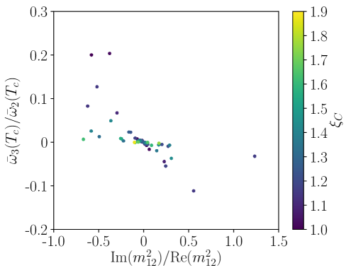
Figure 1: Type I, $H_{1}=h$: The value $\bar{\omega}_{3}(T_{c})/\bar{\omega}_{2}(T_{c})$ at the critical temperature $T_{c}$ versus $\mbox{Im}(m_{12}^{2})/\mbox{Re}(m_{12}^{2})\neq 0$ at $T=0$ for points with a strong PT. The colour code indicates the size of $\xi_{c}$.

The colour code indicates the value of $\xi_{c}$. Note that in Fig. 1 we only plot C2HDM parameter points, i.e. $\mbox{Im}(m_{12}^{2})/\mbox{Re}(m_{12}^{2})\neq 0$, although this ratio can become very small. As can be inferred from the figure, the phase $\varphi^{\text{spont}}$ of spontaneous CP violation and the one of explicit CP violation, $\varphi^{\text{explicit}}$, are correlated. A CP-violating phase at $T_{c}$ is generated spontaneously only if already in the zero-temperature potential there is non-vanishing CP violation. As we set the CKM matrix to unity in the computation of the effective potential no CP violation can be generated through loop effects if CP is conserved at $T=0$. The size of $\xi_{c}$ is not correlated to the size of the CP-violating phase. We observe, however, that the maximum obtained value of $\xi_{c}$, which quantifies the strength of the PT, is $\xi_{c}=1.89$. This is below the value found in the CP-conserving 2HDM, cf. Ref. [51] and the following section.

Figure 2 shows the development of the VEVs exemplary for one parameter point, defined by

$$\begin{array}[]{lll}M_{H_{1}}=125.09\mbox{ GeV},&\qquad M_{H_{2}}=163.119\mbox{ GeV},&\\ M_{H_{3}}=387.461\mbox{ GeV},&\qquad M_{H^{\pm}}=393.035\mbox{ GeV},\\ \alpha_{1}=1.1376,&\qquad\alpha_{2}=0.0601,&\qquad\alpha_{3}=-0.0934,\\ \tan\beta=5.6211,&\qquad\mbox{Re}(m_{12}^{2})=4341\mbox{ GeV}^{2}\;.\end{array}$$ (105)

We observe, in the upper left plot the generation of the VEV $v=\sqrt{\bar{\omega}_{1}^{2}+\bar{\omega}_{2}^{2}+\bar{\omega}_{3}^{2}}$ ($\bar{\omega}_{3}\equiv\bar{\omega}_{\text{CP}}$) at $T_{c}=136.011$ GeV with a value of $v_{c}=156.245$ GeV and hence $\xi_{c}=1.149$. With decreasing temperature the VEV increases to the value 246 GeV at $T=0$. Note, that the VEV also includes $\bar{\omega}_{\text{CB}}$, which, however, always turns out to be zero, so that we did not write it explicitly here. The upper right and lower left plots show the development of the absolute values of the individual VEVs, i.e. the ones of $\bar{\omega}_{1}$ and $\bar{\omega}_{2}$, the CP-conserving VEVs coinciding with $v_{1}$ and $v_{2}$ at zero temperature, and of the CP-violating VEV $\bar{\omega}_{3}$. We also show, in the lower right plot, the development of $\bar{\omega}_{3}/\bar{\omega}_{2}$. Because of the value of $\tan\beta$ above 1, the value $|\bar{\omega}_{2}|$ is larger than $|\bar{\omega}_{1}|$. The spontaneously generated CP-violating VEV $\bar{\omega}_{3}$ at the PT amounts with $|\bar{\omega}_{3}(T_{c})|=17.06$ to 11% of the absolute value of $\bar{\omega}_{2}$ and decreases monotonously to zero with decreasing temperature, while $\bar{\omega}_{1}$ and $\bar{\omega}_{2}$ monotonously increase to reach $\sqrt{\bar{\omega}_{1}^{2}+\bar{\omega}_{2}^{2}}(T=0)=246$ GeV.

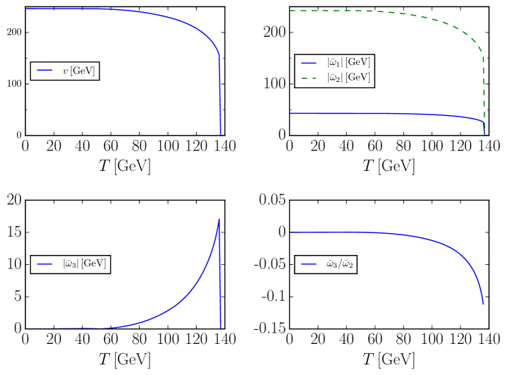
Figure 2: Type I, $H_{1}=h$: The development of the VEV as a function of the temperature. In clockwise direction: the total VEV $v$; the absolute values of the CP-conserving VEVs, $|\bar{\omega}_{1}|$ (blue/full) and $|\bar{\omega}_{2}|$ (green/dashed), the absolute value of the CP-violating VEV, $|\bar{\omega}_{3}|$, and $\bar{\omega}_{3}/\bar{\omega}_{2}$.

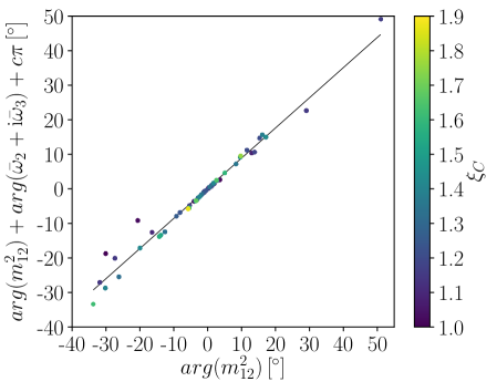
Figure 3: Type I, $H_{1}=h$: The total CP-violating angle at the critical temperature $T_{c}$ versus the CP-violating angle at $T=0$. By adding $c\pi$, $c\in\{-1,0,1\}$, the angle is ensured to lie in the range $-90^{\circ}$ to $90^{\circ}$. The colour code indicates the size of $\xi_{c}$.

Figure 3 shows the total CP-violating angle at the PT as a function of the CP-violating angle at $T=0$. The former varies between about -34^∘ and 49^∘ for CP-violating angles of -35^∘ to 51^∘ allowed at $T=0$. We observe almost maximal CP violation which should be enough for successful baryogenesis [10, 43].

6.2 Implications for LHC phenomenology and benchmark scenarios

Figure 4 shows the mass of the heavier non-SM-like Higgs boson, $m_{\uparrow}$, versus the lighter one, $m_{\downarrow}$, where the grey points pass the applied constraints and include both CP-conserving and CP-violating points in the left plot, but only CP-violating points in the right plot. The coloured points additionally feature a strong first order PT. The maximum possible value of $\xi_{c}$ is found to be $\xi_{c}=5.7$ for all 2HDM points (left plot). If we only consider CP-violating points (right plot) the number of grey points is reduced. The number of points compatible with a strong PT is reduced even more, with the maximally allowed $\xi_{c}$ being 1.89. The mass plots show that the requirement of a strong PT overall prefers somewhat lighter non-SM-like Higgs bosons. The allowed maximum masses are further reduced in case of CP violation where $m_{\uparrow}$ remains below about 753 GeV and $m_{\downarrow}$ does not exceed 636 GeV. Through the CP mixing all Higgs bosons participate in the PT, also the heavier ones. Additionally, a CP-violating VEV $\bar{\omega}_{3}$ is generated at $T_{c}$ and feeds into the VEV of also the heavier Higgs bosons. With heavier Higgs bosons participating in the PT, the PT is weakened inducing smaller $\xi_{c}$ values. In order to counterbalance these effects, the Higgs masses overall become lighter and/or they move closer together (cf. the coloured points on the diagonal axis), thus also distributing large portions of the VEV to the lighter among the Higgs bosons.

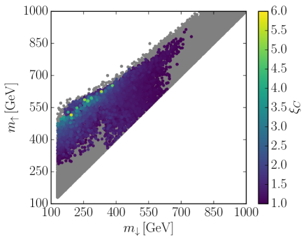
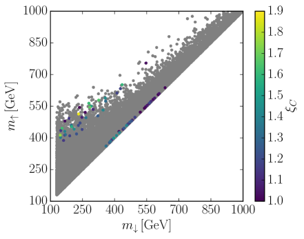
Figure 4: Type I, $H_{1}=h$: The mass of the heavier versus the lighter non-SM-like Higgs boson. Left: CP-conserving and CP-violating points, right: only CP-violating points. Grey: points passing all the constraints; color: points with additionally $\xi_{c}\geq 1$. The color code indicates the value of $\xi_{c}$.

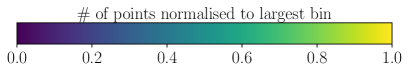
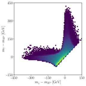
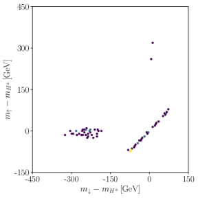
Figure 5: Type I, $H_{1}=h$: The mass difference $m_{\uparrow}-m_{H^{\pm}}$ versus $m_{\downarrow}-m_{H^{\pm}}$. The colour code shows the relative frequency of left: all points passing the constraints; middle: all points with a strong PT and CP conservation; right: all points with $\xi_{c}\geq 1$ and explicit CP violation.

In Fig. 5 we investigate how a strong PT affects LHC phenomenology. The left plot shows in the plane $(m_{\uparrow}-m_{H^{\pm}})$ versus $(m_{\downarrow}-m_{H^{\pm}})$ the frequency of the points that pass the constraints, the middle and right plot display the frequency of the points when additionally a strong EWPT is required and only the CP-conserving points (middle) or the CP-violating points (right) are taken into account. The LHC constraints favour degenerate non-SM-like neutral Higgs bosons that are lighter (by at most 70 GeV) or equal to the charged Higgs boson mass, cf. yellow points in Fig. 5 (left). In the CP-conserving case, a strong PT, however, favours a hierarchy between the neutral masses, see Fig. 5 (middle): While the heavier $H_{\uparrow}$ is approximately mass degenerate with the charged Higgs, $H_{\downarrow}$ is lighter by about 200 GeV. A slight preference is also found for mass degenerate $H_{\downarrow}$ and $H^{\pm}$ with $H_{\uparrow}$ being heavier by 250-350 GeV.

As can be inferred from the comparison of the middle and right plot, most of the points with a strong PT are found in the CP-conserving limit, and we find that the strongest PT is obtained in the alignment limit where $H_{1}$ is totally SM-like. In line with Ref. [51] we hence conclude, that a strong PT favours scenarios where decays of the heavier neutral Higgs boson into the lighter one together with a $Z$ boson are kinematically allowed and may have a considerable branching ratio due to the involved coupling being large in the alignment limit. We also find that the mass configuration with a mass gap of 290-330 GeV between $H_{\downarrow}$ and $H_{\uparrow}$ induces the largest $\xi_{c}$ values (not shown in the plots). When keeping only the CP-violating points (right plot), we find three different types of mass configurations that are compatible with a strong PT. $(i)$ We have the parameter sets where $H_{\uparrow}$ and $H^{\pm}$ are approximately mass degenerate with $H_{\downarrow}$ being lighter by 180 to 320 GeV. $(ii)$ We find two points with mass degenerate $H_{\downarrow}$ and $H^{\pm}$ and $H^{\uparrow}$ begin heavier by 280 GeV and 330 GeV, respectively. $(iii)$ Finally, $H_{\downarrow}$ and $H_{\uparrow}$ are approximately mass degenerate and $H^{\pm}$ is either lighter, heavier or has the same mass. We investigate the features of these points closer by identifying benchmark points for each of these regions. We denote these points by BPi1-3, BPii1-2 and BPiii1-3 for three mass configuration types $(i)$, $(ii)$ and $(iii)$, respectively. In Tables 2, 4 and 6 we list the input parameters of the 3 sets of benchmarks. We also give the derived third neutral Higgs boson mass, the strength of the PT $\xi_{c}$ and the CP admixtures of the Higgs bosons. These are quantified by the mixing matrix element squared relating to the CP-odd neutral component of the Higgs doublets $\zeta_{3}$, namely $R_{i3}^{2}$ ($i=1,2,3$). Finally, we give for all benchmark points the result for the production of a SM-like Higgs pair $h$ through gluon fusion at a c.m. energy of $\sqrt{s}=14$ TeV including the NLO QCD corrections in the heavy top mass limit [121]. We come back to the discussion of Higgs pair production in Section 7. In Tables 3, 5 and 7 we summarise the dominant branching ratios of the benchmark points of the three sets, which determine their phenomenology. For $H_{1}$ we have SM-like branching ratios and do not give them separately here.

	BPi1	BPi2	BPi3
$m_{H_{1}}$ [GeV]	125.09	125.09	125.09
$m_{H_{2}}$ [GeV]	322.28	291.49	188.52
$m_{H^{\pm}}$ [GeV]	522.12	543.30	490.97
$\mbox{Re}(m_{12}^{2})$ [GeV2]	17100	15590	9053
$\alpha_{1}$	1.484	1.366	1.548
$\alpha_{2}$	-0.018	-0.028	-0.085
$\alpha_{3}$	0.112	0.086	0.999
$\tan\beta$	5.97	5.08	19.97
$m_{H_{3}}$ [GeV]	503.15	548.97	491.27
$\xi_{c}$	1.26	1.52	1.15
$R_{13}^{2}$	$3.284\cdot 10^{-4}$	$7.641\cdot 10^{-4}$	$7.219\cdot 10^{-3}$
$R_{23}^{2}$	$0.012$	$7.436\cdot 10^{-3}$	0.702
$R_{33}^{2}$	0.987	0.992	0.291
$\sigma_{hh}^{\text{NLO}}$ [fb]	89.14	217.95	38.42

Table 2: Line 1-8: The input parameters of the benchmark points BPi1-3. Line 9 to 13: The derived 3rd neutral Higgs boson mass, the $\xi_{c}$ value and the CP-odd admixtures $R_{i3}^{2}$. Line 14: The NLO QCD gluon fusion $hh$ production cross section at $\sqrt{s}=14$ TeV.

	BPi1	BPi2	BPi3
BR($H_{2}$)	BR($H_{2}\to H_{1}H_{1}$) = 0.526	BR($H_{2}\to H_{1}H_{1}$) = 0.400	BR($H_{2}\to WW$) = 0.787
	BR($H_{2}\to WW$) = 0.310	BR($H_{2}\to ZH_{1}$) = 0.294	BR($H_{2}\to ZZ$) = 0.196
	BR($H_{2}\to ZZ$) = 0.140	BR($H_{2}\to WW$) = 0.156	BR($H_{2}\to b\bar{b}$) = 0.010
BR($H_{3}$)	BR($H_{3}\to ZH_{2}$) = 0.866	BR($H_{3}\to ZH_{2}$)=0.940	BR($H_{3}\to ZH_{2}$) = 0.982
	BR($H_{3}\to t\bar{t}$) = 0.100	BR($H_{3}\to t\bar{t}$)=0.056	BR($H_{3}\to WW$) = 0.0075
	BR($H_{3}\to ZH_{1}$) = 0.028	BR($H_{3}\to WW$)=0.002	BR($H_{3}\to ZH_{1}$) = 0.0044
BR($H^{\pm}$)	BR($H^{\pm}\to WH_{2}$) = 0.906	BR($H^{\pm}\to WH_{2}$)=0.943	BR($H^{\pm}\to WH_{2}$) = 0.987
	BR($H^{+}\to t\bar{b}$) = 0.069	BR($H^{+}\to t\bar{b}$)=0.054	BR($H^{\pm}\to WH_{1}$) = 0.011
	BR($H^{\pm}\to WH_{1}$) = 0.025	BR($H^{\pm}\to WH_{1}$)=0.002	BR($H^{+}\to t\bar{b}$) = 0.0025

Table 3: The dominant branching ratios of the BPi1-3 Higgs bosons.

	BPii1	BPii2
$m_{H_{1}}$ [GeV]	125.09	125.09
$m_{H_{2}}$ [GeV]	263.77	236.99
$m_{H^{\pm}}$ [GeV]	257.64	223.76
$\mbox{Re}(m_{12}^{2})$ [GeV2]	13823	8044
$\alpha_{1}$	1.497	1.287
$\alpha_{2}$	$4.741\cdot 10^{-3}$	-0.050
$\alpha_{3}$	-0.021	0.127
$\tan\beta$	4.90	6.95
$m_{H_{3}}$ [GeV]	519.75	542.95
$\xi_{c}$	1.02	1.003
$R_{13}^{2}$	$2.247\cdot 10^{-5}$	$2.459\cdot 10^{-3}$
$R_{23}^{2}$	$4.545\cdot 10^{-4}$	$0.016$
$R_{33}^{2}$	0.999	0.981
$\sigma_{hh}^{\text{NLO}}$ [fb]	68.28	30.73

Table 4: Line 1-8: The input parameters of the benchmark points BPii1 and BPii2. Line 9 to 13: The derived 3rd neutral Higgs boson mass, the $\xi_{c}$ value and the CP-odd admixtures $R_{i3}^{2}$. Line 14: The NLO QCD gluon fusion $hh$ production cross section at $\sqrt{s}=14$ TeV.

We start our discussion with the benchmark set BPi1-3. Denoting by $\phi$ the heavier mass degenerate Higgs bosons $H_{\uparrow}=H_{3}$ and $H^{\pm}$, the three benchmarks differ in the their mass difference $m_{\phi}-m_{H_{\downarrow}=H_{2}}$ which is about 200, 250 and 300 GeV for BPi1, BPi2 and BPi3. Since the masses of the heavier Higgs bosons $\phi$ are between about 490 and 550 GeV in all three scenarios, this means that $m_{\downarrow}$ becomes successively smaller with increasing mass difference. The interplay of the kinematically available phase space and the CP nature of the Higgs bosons determines their branching ratios. In particular, the decays of $H_{\downarrow}\equiv H_{2}$ turn out to be interesting. In BPi1 and BPi2, where $H_{2}$ is mainly CP-even, it is heavy enough to decay with substantial branching ratio into a SM-like Higgs pair $H_{1}=h$. Since in BPi2 the coupling to massive gauge bosons is smaller than in BPi1, the next important decay in BPi1 is into $WW$, while in BPi2 it is into $H_{1}Z$. Although the coupling is $H_{1}H_{2}Z$ is rather small, because both $H_{1}$ and $H_{2}$ are mostly CP-even, the decay is important as all the other decays involve even smaller couplings or are kinematically closed. Note, in particular, that in the CP-conserving 2HDM this decay would be forbidden. Since $H_{2}$ also decays with a branching ratio of 0.156 into $WW$ the CP-violating nature of $H_{2}$ can be identified at the LHC through its decay rates: Due to the fact that we know already that $H_{1}\equiv h$ is mainly CP-even, as it corresponds to the discovered Higgs boson, the properties of which have been determined, the observation of the $H_{2}$ decay both into $WW$ and $ZH_{1}$ clearly identifies it to be CP-violating. This idea has been proposed and discussed before in[122, 123]. The reason is that the former decay requires $H_{2}$ to be CP-even, whereas the latter requires it to be CP-odd in a purely CP-conserving theory. In BPi3, $H_{2}$ has a large CP-odd admixture. Due to its small mass, however, the off-shell decay into $ZH_{1}$ is less important than the on-shell decays into massive gauge bosons. Here we make the interesting observation that $H_{2}$, despite its rather CP-odd nature, mainly decays into massive gauge bosons as a consequence of the available phase space. These decays are only possible because $H_{2}$ also has a CP-even admixture. The heavier non-SM-like Higgs $H_{\uparrow}\equiv H_{3}$ in all three scenarios mainly decays into $ZH_{2}$. In BPi1 and BPi2, where $H_{3}$ is mainly CP-odd, the next important decay is the one into top-quark pairs. In BPi3 $H_{3}$ is more CP-even, so that the second important decay becomes the one into $WW$. Note, that the decay into $ZH_{1}$ is less important than into $ZH_{2}$ because of a much smaller involved coupling. In our scenarios, the coupling of $H^{\pm}$ to $WH_{1}$ is smaller than the one to $WH_{2}$, so that the charged Higgs decays mainly into $WH_{2}$ followed by the decay into $t\bar{b}$ in BPi1 and BPi2 and by $WH_{1}$ in BPi3.

	BPii1	BPii2
BR($H_{2}$)	BR($H_{2}\to WW$) = 0.464	BR($H_{2}\to WW$) = 0.698
	BR($H_{2}\to H_{1}H_{1}$) = 0.336	BR($H_{2}\to ZZ$) = 0.289
	BR($H_{2}\to ZZ$) = 0.199	BR($H_{2}\to b\bar{b}$) = 0.005
BR($H_{3}$)	BR($H_{3}\to W^{\pm}H^{\mp}$) = 0.672	BR($H_{3}\to W^{\pm}H^{\mp}$)=0.685
	BR($H_{3}\to ZH_{2}$) = 0.297	BR($H_{3}\to ZH_{2}$)=0.297
	BR($H_{3}\to t\bar{t}$) = 0.019	BR($H_{3}\to ZH_{1}$)=0.011
BR($H^{\pm}$)	BR($H^{+}\to t\bar{b}$) = 0.923	BR($H^{+}\to t\bar{b}$)=0.924
	BR($H^{\pm}\to WH_{1}$) = 0.075	BR($H^{\pm}\to WH_{1}$)=0.074

Table 5: The dominant branching ratios of the BPii1 and BPii2 Higgs bosons.

The benchmark points BPii1 and BPii2 are rather similar. They differ in the mass gap between the heavier $H_{\uparrow}\equiv H_{3}$ and the lighter $H_{\downarrow}\equiv H_{2}$, which is now almost mass degenerate with $H^{\pm}$. Denoting the latter two by $\varphi$, we have $m_{H_{\uparrow}}-m_{\varphi}\approx 260$ GeV in BPii1 and around 310 GeV in BPii2, where $H_{\downarrow}$ and $H^{\pm}$ are lighter than in BPii1. In both scenarios $H_{1}\equiv h$ and $H_{\downarrow}$ are mostly CP-even and $H_{\uparrow}$ is mostly CP-odd. Therefore, $H_{2}$ mainly decays into the massive gauge bosons, cf. Table 5. In BPii1 also the decay into $H_{1}H_{1}$ has a substantial branching ratio of 0.34. In BPii2, this decay is kinematically closed. The dominant decays of $H_{3}$, which is now heavier than $H^{\pm}$, are into a gauge+Higgs boson final state, namely into $W^{\pm}H^{\mp}$ and $ZH_{2}$ with branching ratios of about 0.7 and 0.3 in both scenarios. In contrast to the parameter set $(i)$, the charged Higgs boson is considerably lighter, so that it mainly decays into $t\bar{b}$ and the decay into a gauge+Higgs final state is very small. Again, we find non-SM-like decays in these scenarios, where the possible final states reflect the mass hierarchy among the Higgs bosons. Note, finally, that both benchmark points have a $\xi_{c}$ just slightly above the strong PT value of $\xi_{c}=1$ and are almost ruled out.

	BPiii1	BPiii2	BPiii3
$m_{H_{1}}$ [GeV]	125.09	125.09	125.09
$m_{H_{2}}$ [GeV]	494.834	420.481	460.698
$m_{H^{\pm}}$ [GeV]	503.432	499.906	385.220
$\mbox{Re}(m_{12}^{2})$ [GeV2]	39529	27614	20392
$\alpha_{1}$	0.920	0.957	0.932
$\alpha_{2}$	$9.303\cdot 10^{-3}$	0.012	0.0101
$\alpha_{3}$	-0.461	-0.131	-0.514
$\tan\beta$	1.488	1.851	1.608
$m_{H_{3}}$ [GeV]	496.683	429.492	462.683
$\xi_{c}$	1.18	1.03	1.21
$R_{13}^{2}$	$8.655\cdot 10^{5}$	$1.391\cdot 10^{-4}$	$1.011\cdot 10^{-4}$
$R_{23}^{2}$	0.198	0.0170	0.241
$R_{33}^{2}$	0.802	0.983	0.748
$\sigma_{hh}^{\text{NLO}}$ [fb]	36.05	47.85	31.66

Table 6: Line 1-8: The input parameters of the benchmark points BPiii1-3. Line 9 to 13: The derived 3rd neutral Higgs boson mass, the $\xi_{c}$ value and the CP-odd admixtures $R_{i3}^{2}$. Line 14: The NLO QCD gluon fusion $hh$ production cross section at $\sqrt{s}=14$ TeV.

	BPiii1	BPiii2	BPiii3
BR($H_{2}$)	BR($H_{2}\to t\bar{t}$) = 0.972	BR($H_{2}\to t\bar{t}$) = 0.860	BR($H_{2}\to t\bar{t}$) = 0.948
	BR($H_{2}\to WW$) = 0.015	BR($H_{2}\to WW$) = 0.089	BR($H_{2}\to WW$) = 0.027
	BR($H_{2}\to ZZ$) = 0.007	BR($H_{2}\to ZZ$) = 0.042	BR($H_{2}\to ZZ$) = 0.013
BR($H_{3}$)	BR($H_{3}\to t\bar{t}$) = 0.984	BR($H_{3}\to t\bar{t}$)= 0.951	BR($H_{3}\to t\bar{t}$) = 0.969
	BR($H_{3}\to Zh$) = 0.010	BR($H_{3}\to Zh$) = 0.044	BR($H_{3}\to Zh$) = 0.018
BR($H^{\pm}$)	BR($H^{+}\to t\bar{b}$) = 0.987	BR($H^{+}\to t\bar{b}$)= 0.932	BR($H^{+}\to t\bar{b}$) = 0.985
	BR($H^{\pm}\to Wh$) = 0.011	BR($H^{\pm}\to Wh$) = 0.065	BR($H^{\pm}\to Wh$) = 0.013

Table 7: The dominant branching ratios of the BPiii1-3 Higgs bosons.

We find four scenarios for which all non-SM-like Higgs bosons are approximately mass degenerate. Denoting by $\Phi$ generically $H_{\downarrow}$, $H_{\uparrow}$ and $H^{\pm}$, we have for their average mass $m_{\Phi}\approx 498$ GeV, $547$ GeV, $555$ GeV and 563 GeV, respectively, for these scenarios. All four scenarios feature the same dominant branching ratios. We exemplary give as benchmark point BPiii1 the scenario with the lightest mass spectrum. The two other benchmark points feature $m_{\downarrow}\approx m_{\uparrow}$, where the charged Higgs boson is heavier (BPiii2) or lighter (BPiii3). In BPiii1, there is no mass gap between the non-SM-like Higgs bosons, and in BPiii2 and BPiii3 the largest mass gap is 80 and 77 GeV, respectively. Furthermore, in all these scenarios the couplings between $H_{2,3}$, $Z$ and $h$ are small. Therefore the non-SM-like Higgs bosons decay dominantly into SM final states, which due to their mass values are $t\bar{t}$ for the neutral Higgs bosons and $t\bar{b}$ for the charged Higgs boson. For $H_{2}$ which has a significant CP-odd admixture but still is dominantly CP-even, the next important decay channels are those into $WW$ and $ZZ$.

We can therefore summarise that the requirement of a strong PT induces Higgs spectra with mass gaps that are characterized by large Higgs branching ratios of the non-SM-like Higgs bosons into gauge+Higgs final states or into Higgs pairs which should be testable at the LHC. Some of the decays of our scenarios would be forbidden in a purely CP-conserving 2HDM. In contrast to the CP-conserving case, due to the CP-mixing of all Higgs bosons, also scenarios with the non-SM-like Higgs bosons being close in mass or even mass degenerate are preferred. In these cases the dominant decays are those into SM final states.

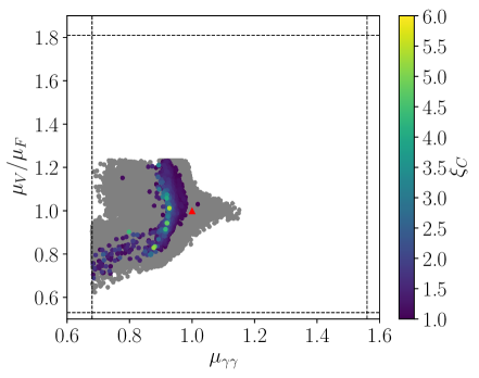
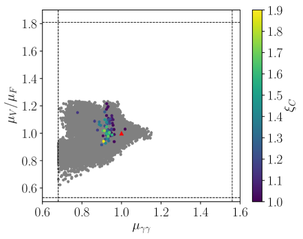
Figure 6: Type I, $H_{1}=h$: $\mu_{V}/\mu_{F}$ versus $\mu_{\gamma\gamma}$. Grey: all points passing the applied constraints, colour: all points with additionally $\xi_{c}\geq 1$; left: all 2HDM points, right: only C2HDM points. The red triangle marks the SM result.

Figure 6 shows in grey the distribution of the Higgs signal strengths for the scenarios passing the constraints and in colour the ones that are additionally compatible with a strong PT. The fermion initiated cross section (gluon fusion and associated production with a heavy quark pair) of the SM-like Higgs boson $h$ normalised to the SM is denoted by $\mu_{F}$, and the normalised production cross section through massive gauge bosons (gauge boson fusion and associated production with a vector boson) by $\mu_{V}$. The value $\mu_{xx}$ is defined as

$$\mu_{xx}=\mu_{F}\frac{\mbox{BR}_{\text{C2HDM}}(h\to xx)}{\mbox{BR}_{\text{SM}}(H_{\text{SM}}\to xx)}\;,$$ (106)

where $H_{\text{SM}}$ is the SM Higgs boson with mass 125 GeV. In the right plot we retained only the points with explicit CP violation. Photonic rates of up to 1.15 are still allowed. When imposing a strong PT, however, this reduces to 1.02 for parameter points with CP violation and below 1 for CP-conserving scenarios. Note that we did not find any points with both reduced $\mu_{V}/\mu_{F}$ and $\mu_{\gamma\gamma}$ by more than 10% that lead to $\xi_{c}\geq 1$ in the CP-violating case.

In Fig. 7 we see in the $\mu_{\tau\tau}-\mu_{VV}$ plane the distribution of points passing the constraints and how this compares to the points when we require a strong PT (left) and only keep those points that are CP-violating and feature $\xi_{c}\geq 1$ (right). Clearly, in the CP-violating case the points with a strong PT are much more sparse and disfavour points with $\mu_{\tau\tau}$ above the SM value of 1 and reduced $\mu_{VV}$. The differences in the rates that we found can be exploited to distinguish the C2HDM from the R2HDM or to exclude the C2HDM.

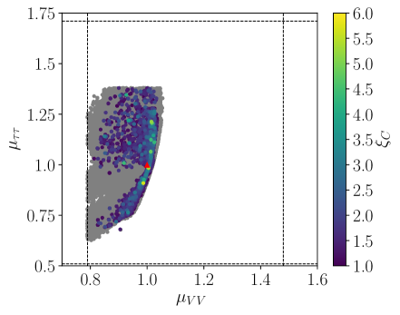
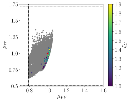
Figure 7: Type I, $H_{1}=h$: $\mu_{\tau\tau}$ versus $\mu_{VV}$. Grey: all points passing the applied constraints, colour: all points with additionally $\xi_{c}\geq 1$; left: all 2HDM, right: only C2HDM points. The red triangle marks the SM result.

7 Analysis of the trilinear Higgs self-couplings and Higgs pair production in the C2HDM Type I

Having computed the loop-corrected effective potential at finite temperature, we now investigate the effects of the NLO corrections on the trilinear Higgs self-coupling as well as the interplay between a strong PT and the trilinear Higgs self-couplings. The loop-corrected trilinear Higgs self-couplings are obtained from the loop-corrected effective potential by performing the third derivative of the Higgs potential with respect to the Higgs fields. The problem of infrared divergences related to the Goldstone bosons in the Landau gauge is treated analogously to the extraction of the masses from the second derivative of the potential [93].

7.1 The Higgs self-coupling between three SM-like Higgs bosons

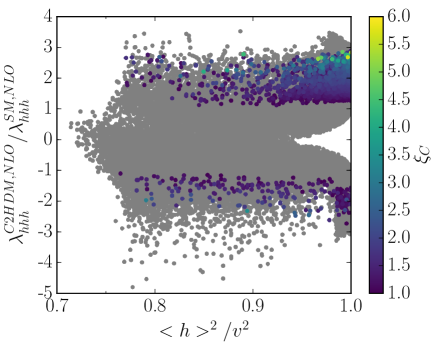
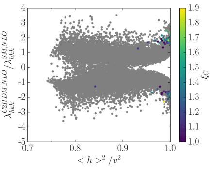
Figure 8: Type I, $H_{1}=h$: The C2HDM trilinear Higgs self-coupling between three SM-like Higgs bosons $h$ normalized to the SM value, at NLO, as function of the fraction of the VEV squared carried by $h$. Grey: all points passing the constraints; colour: points with additionally $\xi_{c}\geq 1$. Left: all 2HDM points; right: only the C2HDM points.

In Fig. 8 we show the NLO trilinear Higgs coupling between three SM-like Higgs bosons $h$ of the C2HDM normalized to the SM value, each at NLO, as function of the fraction of the VEV squared (indicated by the brackets) carried by $h$. The left plot comprises all 2HDM points, while the right one only those with explicit CP violation at $T=0$. For the NLO SM value of the self-coupling we use the formula given in [125] that takes into account the dominant top-quark contributions at NLO. The grey points of the left plot show that in the 2HDM the trilinear coupling can substantially deviate from the SM value and both be suppressed or enhanced compared to the SM, i.e. the present constraints do not restrict this coupling to be close to the SM value. The maximum enhancement factor is $\pm 4.9$ (without the NLO unitarity constraints it would be 8). When requiring a strong PT the enhancement is smaller, with $\lambda_{hhh}^{\text{C2HDM,NLO}}/\lambda_{hhh}^{\text{SM,NLO}}\approx(-2.73...-1.1)$ and $(1.1...2.9)$. Still, a strong PT clearly requires a large enough Higgs self-coupling, larger than the one realized in the SM. Along these lines, we see that the largest $\xi_{c}$ values are obtained for the largest enhancement factors in this range. Including only points with explicit CP violation the maximum enhancement factor is found to be $\sim 3.6$ for all points passing the constraints. The scenarios with $\xi_{c}>1$ reduce the maximum enhancement factor somewhat with $\lambda_{hhh}^{\text{C2HDM,NLO}}/\lambda_{hhh}^{\text{SM,NLO}}\approx(-2.30...-1.28)$ and $(1.26...2.46)$. The upper bound on the trilinear coupling is given by the interplay between the quartic self-couplings of the potential and the masses of the Higgs bosons participating in the EWPT, with the latter weakening the strength of the phase transition for too large mass values. Therefore, for $\xi_{c}\geq 1$ and CP violation, the ratio of the VEV carried by the lighter of the non-SM-like Higgs bosons, $H_{\downarrow}$, can be up to about $0.4\,v$, in contrast to the heavier $H_{\downarrow}$ with $\langle H_{\uparrow}\rangle=0.12\,v$ at most. The larger the fraction of the VEV carried by the Higgs boson, the stronger is its participation in the EWPT, so that it should not be too heavy in order not to spoil the strong PT. The largest fraction of the VEV is carried by $h$, with $<h>=(0.87...1)\,v$. The largest $\xi_{c}$ values are obtained in the alignment limit, which is preferred by a strong PT, where the SM-like Higgs boson carries the entire VEV. In this case the remaining two neutral Higgs bosons do not take part in the PT, so that a strong first order PT requires a substantial trilinear Higgs self-coupling for $h$. A conservative estimate of the prospects of the high-luminosity LHC to measure the trilinear Higgs self-coupling of the SM, concludes that an accuracy of about 50% on its value might be feasible [126]. This allows to distinguish some of the C2HDM scenarios compatible with a strong PT from the SM case.

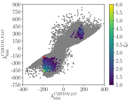
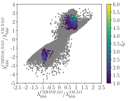
Figure 9: Type I, $H_{1}=h$: Left: The NLO C2HDM trilinear Higgs self-coupling between three SM-like Higgs bosons versus the LO value. The red triangle marks the SM point. Right: The ratio of the C2HDM trilinear Higgs self-coupling between three SM-like Higgs bosons and the SM counterpart at NLO versus the LO ratio. Grey: all points passing the constraints; colour: points with additionally $\xi_{c}\geq 1$. Both plots: all 2HDM points.

The impact of the NLO corrections on the trilinear Higgs self-coupling between three SM-like Higgs bosons in the C2HDM is shown by Fig. 9. The left plot shows the NLO coupling as function of the leading order (LO) coupling. The NLO corrections can both suppress and enhance the tree-level coupling. The corrections can be substantial. For the points with a strong PT, the increase can be by up to a factor 8.3, while it is 2.5 for the parameter point with the largest $\xi_{c}$. As outlined in [125], large corrections, beyond the top loop contribution also present in the SM, arise from Higgs loop contributions in the 2HDM. They increase with the fourth power of the Higgs boson mass, $m_{\Phi}^{4}$, where $\Phi$ stands generically for the 2HDM Higgs bosons $H,A,H^{\pm}$. And they are suppressed by

$$(1-M^{2}/m_{\Phi}^{2})^{3}\;,$$ (107)

with $M^{2}\equiv m_{12}^{2}/(\sin\beta\cos\beta)$. The masses of the heavy Higgs bosons schematically take the form

$$m_{\Phi}^{2}=M^{2}+f(\lambda_{i})v^{2}+{\cal O}(v^{4}/M^{2})\;,$$ (108)

where $f(\lambda_{i})$ denotes a linear combination of the quartic couplings of the Higgs potential. In case of small $M^{2}$ large Higgs masses are generated through large values of $\lambda_{i}$. In this case the loop contributions to the Higgs bosons do not decouple and increase with $m_{\Phi}$, see also [127]. In case $M^{2}\gg f(\lambda_{i})v^{2}$ the loop contributions decouple in the limit $m_{\Phi}^{2}\approx M^{2}\to\infty$ due to the suppression factor Eq. (107). For a strong PT we need large Higgs boson self-couplings, respectively large couplings $\lambda_{i}$, inducing the observed large corrections in the non-decoupling regime. On the other hand, the masses of the Higgs bosons participating in the EWPT should not become too heavy, thus restricting the size of the quartic couplings and hence also of the enhancement through the NLO corrections. This explains why in the regime compatible with a strong PT the enhancement of $\lambda_{hhh}$ remains below the maximum enhancement factor compatible with the applied constraints. The right plot of Fig. 9 displays the ratio between the C2HDM coupling and the SM counterpart at NLO versus this ratio at LO. The NLO ratio deviates substantially from the LO ratio for a large fraction of the parameter points, showing that the NLO effects in the two models can be quite different. This was to be expected as in the C2HDM further Higgs bosons contribute to the loop corrections and their impact can be quite sizeable due to large Higgs self-couplings and/or light masses. Inspecting only pure CP-violating scenarios, we find overall less scenarios compatible with the constraints and a strong PT and the size of the NLO corrections is somewhat reduced.

7.1.1 The benchmark scenario BP3HSM

To quantify the impact of the PT on the Higgs self-coupling and on Higgs pair production, we exemplary give one benchmark point in the CP-violating case, BP3HSM, with the input parameters ($M_{H_{3}}$ is derived from the input parameters)

$$\begin{array}[]{llll}\mbox{\text@underline{BP3HSM:}}&M_{H_{1}}=125.09\mbox{ GeV},&\qquad M_{H_{2}}=356.779\mbox{ GeV},&\\ &M_{H_{3}}=587.511\mbox{ GeV},&\qquad M_{H^{\pm}}=581.460\mbox{ GeV},\\ &\alpha_{1}=1.470,&\qquad\alpha_{2}=0.0223,&\qquad\alpha_{3}=-0.097,\\ &\tan\beta=4.17,&\qquad\mbox{Re}(m_{12}^{2})=29939\mbox{ GeV}^{2}\;.\end{array}$$ (113)

The strength of the phase transition and the CP-odd admixtures are

$$\xi_{c}=1.43\;,\quad R_{13}^{2}=4.962\cdot 10^{-4}\;,\quad R_{23}^{2}=9.292\cdot 10^{-3}\;,\quad R_{33}^{2}=0.990\;.$$ (114)

This means that $H_{1}$ and $H_{2}$ are mostly CP-even and $H_{3}$ is mostly CP-odd. The main branching ratios of the non-SM-like Higgs bosons are ($H_{\downarrow}=H_{2},H_{\uparrow}=H_{3}$)

$$\mbox{BR}(H_{\uparrow}\to ZH_{\downarrow}) = 0.830\;,\quad\mbox{BR}(H_{\uparrow}\to t\bar{t})=0.102\;,\quad\mbox{BR}(H_{\uparrow}\to Zh)=0.061\;,$$ (115)

$$\mbox{BR}(H_{\downarrow}\to hh) = 0.514\;,\quad\mbox{BR}(H_{\downarrow}\to WW)=0.309\;,\quad\mbox{BR}(H_{\downarrow}\to ZZ)=0.142\;,\quad$$ (116)

$$\mbox{BR}(H^{\pm}\to W^{\pm}H_{\downarrow}) = 0.835\;,\quad\mbox{BR}(H^{+}\to t\bar{b})=0.100\;,\quad\mbox{BR}(H^{\pm}\to W^{\pm}h)=0.065\;,\quad$$ (117)

so that the decays into gauge+Higgs or Higgs pair final states dominate. For this scenario the ratios of the SM-like trilinear Higgs self-coupling to the SM coupling at LO and NLO are

$$\mbox{\text@underline{BP3HSM}}:\quad\frac{\lambda^{\text{C2HDM,LO}}_{hhh}}{\lambda^{\text{SM,LO}}_{hhh}}=0.793\quad\mbox{and}\quad\frac{\lambda^{\text{C2HDM,NLO}}_{hhh}}{\lambda^{\text{SM,NLO}}_{hhh}}=2.135\;,$$ (118)

with the NLO to LO C2HDM coupling ratio being

$$\frac{\lambda^{\text{C2HDM,NLO}}_{hhh}}{\lambda^{\text{C2HDM,LO}}_{hhh}}=2.438\;,$$ (119)

showing the importance of the loop corrections.

We now discuss the effect of these corrections on continuum Higgs pair production. At the LHC the dominant process is given by gluon fusion [128, 129, 121, 126]. The contributing diagrams are the triangle diagrams with the production of a Higgs or $Z$ boson that subsequently decays into a Higgs pair, and the box diagrams [88]. For the NLO cross section of gluon fusion into the SM-like Higgs pair $hh$, computed with a private version of HPAIR [130] adapted for the C2HDM [88], we find at a c.m. energy of 14 TeV

$$\sigma^{\text{NLO}}(pp\to hh)=125.447\mbox{ fb}\;.$$ (120)

The QCD corrections computed in the heavy top mass limit yield a $K$-factor, i.e. a ratio of NLO to LO cross section (the latter calculated with LO strong coupling constant and parton distribution functions), of

$$K=\frac{\sigma^{\text{NLO}}}{\sigma^{\text{LO}}}=1.982\;,$$ (121)

showing the importance of the QCD corrections. The NLO cross section for SM Higgs pair production computed with full top quark mass dependence amounts to [131, 132, 133]

$$\sigma^{\text{NLO}}(H_{\text{SM}}H_{\text{SM}})=32.91\mbox{ fb}\;.$$ (122)

The C2HDM cross section is hence by a factor of 3.8 larger than in the SM. This cross section does not include any EW corrections, and in particular not the ones given in Eq. (119). The enhancement of 3.8 is mostly due to the resonant production of $H_{\downarrow}$ that subsequently decays into an $h$ pair. Without this resonant enhancement the cross section amounts to

$$\sigma^{\text{NLO}}_{\text{w/o }H_{\downarrow}}(pp\to hh)=49.996\mbox{ fb}\;.$$ (123)

The quantification of the effect of the EW corrections requires the complete calculation of the Higgs pair production process at NLO EW, which is clearly beyond the scope of this paper. The computation of the loop-corrected effective trilinear Higgs self-couplings gives a flavour of the importance of the EW corrections and the impact of the EWPT on this value In particular, we note that the increase of the trilinear Higgs self-coupling may also decrease the total size of the cross-section due to the destructive interference between triangle and box diagrams. Electroweak baryogenesis which requires a certain size of the trilinear Higgs self-coupling between the SM-like Higgs bosons in order to be successful hence has a direct influence on the size of resonant and continuum Higgs pair production that is significant enough to be tested at the LHC (and future colliders).

We finish this section by commenting on the size of the Higgs pair production cross sections of the benchmark points given in Tables 2, 4 and 6. As can be inferred from the values given in the tables, Higgs pair production in the C2HDM is significantly enhanced compared to the SM value for scenarios where resonant heavy Higgs production with subsequent decay into $hh$ is kinematically possible. In the scenarios we looked at, the $H_{\uparrow}hh$ couplings is usually very small, so that the main resonant contribution comes from $H_{\downarrow}$ production. In case this is kinematically not allowed or the $H_{\downarrow}hh$ coupling is also small, the cross section value compares to the one of the SM.

7.2 Further Higgs self-couplings

The inspection of the other trilinear Higgs couplings not involving only the SM-like Higgs boson shows the following: The trilinear C2HDM Higgs self-couplings can be suppressed but also be substantially enhanced compared to the SM trilinear coupling and still be compatible with all constraints. The enhancement factor is less important for scenarios that additionally feature a strong PT. However, it can still be considerable, depending on the self-coupling and the scenario. Also the NLO corrections can be important. Barring the case where the LO coupling is close to zero and hence the coupling becomes effectively loop-induced, the maximum enhancement factor for CP-violating scenarios with $\xi_{c}>1$ is 5.7. Due to the large amount of possible trilinear couplings, we exemplary show in Fig. 10 the coupling between the SM-like Higgs boson and $H_{\downarrow}$ and $H_{\uparrow}$, $\lambda_{hH_{\downarrow}H_{\uparrow}}$. For this coupling, the enhancement in the C2HDM compared to the SM coupling can be up to a factor $1.5$ at NLO in accordance with all constraints, cf. Fig. 10 (left). When additionally a strong PT is demanded, the ratio drops to values between -0.34 and 0.47 the SM coupling. The largest $\xi_{c}$ value is obtained close to the alignment limit where $\langle h\rangle\approx v$. The right plot shows the impact of the NLO correction. For the sample compatible with all constraints the ratio of the NLO to the LO coupling can be quite large. The demand of a strong PT has a considerable impact, as in this case the ratio becomes much smaller, as can be inferred from the plot.

8 Type I: Parameter sets with $H_{2}\equiv h$

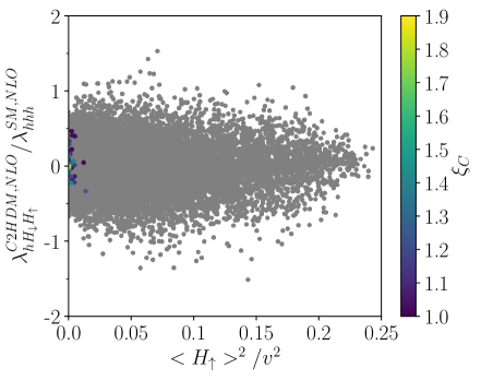
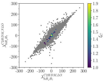
Figure 10: Type I, $H_{1}=h$: Left: The C2HDM trilinear Higgs self-coupling $\lambda_{hH_{\downarrow}H_{\uparrow}}$ normalized to the SM value, at NLO, as a function of the fraction of the VEV squared carried by $H_{\uparrow}$. Right: The NLO C2HDM trilinear coupling $\lambda_{hH_{\downarrow}H_{\uparrow}}$ versus the LO value. Grey: all points passing the constraints; colour: points with additionally $\xi_{c}\geq 1$. Both plots: all 2HDM points.

In this mass configuration our scan resulted in only three scenarios compatible with all constraints that both allow for a strong PT and include CP violation. The results are therefore those of a real 2HDM with the heavier of the two CP-even Higgs bosons being SM-like with a mass of 125 GeV. We reproduced the results of our previous publication on the PT in the CP-conserving 2HDM given in [51], which we briefly summarise here: The scenarios compatible with $\xi_{c}>1$ require (neglecting a few outliers) a mass hierarchy where $H_{\uparrow}$, i.e. the pseudoscalar $A$ in the R2HDM, is mass degenerate with $H^{\pm}$ and lies in the mass range $\sim$130 to $\sim$490 GeV, so that there is a mass gap between $m_{\uparrow}$ and $m_{\downarrow}<125$ GeV. The reason is that due to the required small $m_{\downarrow}$, coinciding with the mass of the lighter of the two CP-even R2HDM Higgs bosons $h$, the quartic coupling $\lambda_{2}$ and $m_{12}^{2}$ have to be small. Hence we are left with $\lambda_{4}$ and $\lambda_{5}$ that drive the phase transition, implying large $H_{\uparrow}$ and $H^{\pm}$ masses and the mass gap to $H_{\downarrow}$. Keeping in mind that $H_{2}$, i.e. the heavier of the 2 CP-even Higgs bosons, is SM-like induces $\sin(\beta-\alpha)=0$ in the limit of the R2HDM, so that this mass hierarchy allows for $A\to hZ$ decays, involving the coupling $g_{AhZ}\sim\cos(\beta-\alpha)$, and can be probed at the LHC. The upper bound on the masses of the heavy Higgs bosons is given by the fact that the Higgs bosons participating in the PT must not be too heavy.

In the CP-violating 2HDM we barely find any points compatible with $\xi_{c}>1$. We have seen that explicit CP violation comes along with spontaneous CP violation at the PT. The thus generated CP-violating VEV at the EWPT feeds into all Higgs bosons as they are all mixing in the CP-violating 2HDM. As the SM-like Higgs boson must not receive a large CP admixture it is either $H_{\downarrow}$ or $H_{\uparrow}$ that develop a non-negligible CP-violating VEV. Due to the above described mass hierarchy with a heavy $H_{\uparrow}$ its VEV should not become too large, however, in order not to weaken the PT. This favours the lighter $H_{\downarrow}$ to receive a more important fraction of the VEV or else a hierarchy where all neutral Higgs bosons are rather light and hence close in mass. Already in the R2HDM we see that such hierarchies together with a strong PT are very rare, so that the scenarios that can be found are very sparse.

The phenomenological implications of the R2HDM are the same as found in [51] with the main feature that there are only very few scenarios with a strong PT that yield photonic rates $\mu_{\gamma\gamma}$ beyond 0.9, although values of up to 1.45 would still be compatible with the applied constraints. In contrast, however, to [51] the rate into $\tau\tau$ can go up to the maximum allowed experimental value of 1.4 also for $\xi_{c}>1$, which is due to different, i.e. newer, limits on $\tan\beta$ applied in this work. The three explicitly CP-violating scenarios lie in the same boundaries for the $\mu$-rates as the ones of the R2HDM. As for the trilinear Higgs self-couplings, the overall picture is the same as in the $H_{1}\equiv h$ case and we content ourselves to summarise the main features in the conclusions.

8.1 Features of the CP-violating scenarios with strong PT

The closer inspection of the 3 CP-violating scenarios reveals that they all feature Higgs spectra with rather close mass values. The largest difference between the heaviest and the lightest Higgs boson mass is 256 GeV. In Table 8 we list the input parameters of the 3 benchmark point scenarios, denoted by BPCPV1-3, featuring a strong PT in the CP-violating case. We additionally give the derived third neutral Higgs boson mass, $\xi_{c}$, the CP admixtures of the Higgs bosons and the SM-like Higgs pair production cross section through gluon fusion. All three scenarios have $\xi_{c}$ values rather close to 1 underlining the difficulty in finding parameter sets inducing a strong PT in case $H_{2}$ is SM-like. In BPCPV1, $H_{3}$ has the largest mass of all three benchmark points with 376 GeV. A strong PT is possible as $H_{3}$ receives a smaller fraction of the VEV than $H_{1}$ and $H_{2}$. In BPCPV2 and 3, all masses are rather close with the mass of $H_{3}$ being below 160 GeV, which now also carries a larger fraction of the VEV.

	BPCPV1	BPCPV2	BPCPV3
$m_{H_{1}}$ [GeV]	119.62	91.31	118.16
$m_{H_{2}}$ [GeV]	125.09	125.09	125.09
$m_{H^{\pm}}$ [GeV]	374.95	191.70	166.56
$\mbox{Re}(m_{12}^{2})$ [GeV2]	1945.7	1124.44	1160.95
$\alpha_{1}$	-0.453769	-0.00591145	-0.223061
$\alpha_{2}$	0.0966953	-0.914279	1.41808
$\alpha_{3}$	0.0658765	-0.185891	0.331065
$\tan\beta$	7.05923	12.3765	19.5889
$m_{H_{3}}$ [GeV]	375.50	141.44	153.63
$\xi_{c}$	1.48	1.02	1.46
$R_{13}^{2}$	$9.2\cdot 10^{-3}$	0.63	0.97
$R_{23}^{2}$	$4.2\cdot 10^{-3}$	0.013	$2.44\cdot 10^{-3}$
$R_{33}^{2}$	0.99	0.36	$2.07\cdot 10^{-2}$
$\sigma_{hh}^{\text{NLO}}$ [fb]	24.58	35.89	37.22

Table 8: Line 1-8: The input parameters of the type I CP-violating benchmarks with $H_{2}\equiv h$ and $\xi_{c}>1$, compatible with all constraints. Line 9 to 13: The derived 3rd neutral Higgs boson mass, the $\xi_{c}$ value and the CP-odd admixtures $R_{i3}^{2}$. Line 14: The NLO QCD gluon fusion $hh$ production cross section at $\sqrt{s}=14$ TeV.

The phenomenological features of the three benchmarks are summarised in Table 9 where we depict the dominant branching ratios of the various Higgs bosons. For $H_{2}$ we have SM-like branching ratios and do not give them separately here.

	BPCPV1	BPCPV2	BPCPV3
BR($H_{1}$)	BR($H_{1}\to b\bar{b}$) = 0.72	BR($H_{1}\to b\bar{b}$) = 0.72	BR($H_{1}\to b\bar{b}$) = 0.68
BR($H_{3}$)	BR($H_{3}\to ZH_{1}$) = 0.88	BR($H_{3}\to WW$)=0.42	BR($H_{3}\to WW$) = 0.77
	BR($H_{3}\to ZH_{2}$) = 0.088	BR($H_{3}\to ZH_{1}$)=0.33	BR($H_{3}\to ZZ$) = 0.080
	BR($H_{3}\to t\bar{t}$) = 0.024	BR($H_{3}\to b\bar{b}$)=0.14	BR($H_{3}\to ZH_{1}$) = 0.072
BR($H^{\pm}$)	BR($H^{\pm}\to WH_{1}$) = 0.88	BR($H^{\pm}\to WH_{1}$)=0.98	BR($H^{\pm}\to WH_{1}$) = 0.94
	BR($H^{\pm}\to WH_{2}$) = 0.089	BR($H^{+}\to t\bar{b}$)=0.018	BR($H^{+}\to t\bar{b}$) = 0.040
	BR($H^{+}\to t\bar{b}$) = 0.027	BR($H^{\pm}\to WH_{3}$)=0.002	BR($H^{\pm}\to WH_{2}$) = 0.012

Table 9: The dominant branching ratios of the BPCPV1-3 Higgs bosons.

The branching ratios are in accordance with the nature of the Higgs bosons. As can be inferred from the $R_{i3}^{2}$ given in Table 8 the lightest Higgs boson of BPCPV1 is mostly CP-even whereas the heaviest one is mostly CP-odd, so that its branching ratios into massive gauge bosons are suppressed. Instead, the large mass gap of more than 250 GeV between $H_{1}$ and $H_{3}$ together with a maximum $ZH_{1}H_{3}$ coupling, since $H_{2}\equiv h$, allows for a large branching ratio into the $ZH_{1}$ final state with 88%. Also the decay into $ZH_{2}$ yields close to 10%. With large branching ratios of $H_{1}$ and $H_{2}$ into $b\bar{b}$ and with the $Z$ boson in the final state this signature can easily be searched for at the LHC. Instead the top pair final state plays a less important role. The charged Higgs boson, which is almost degenerate with $H_{3}$, decays mainly into $WH_{1}$ followed by $WH_{2}$. In the scenario BPCPV2 the masses are overall much closer and both $H_{1}$ and $H_{3}$ have a considerable CP-even admixture. Consequently, $H_{3}$ dominantly decays off-shell into $WW$, with 42%, followed by the off-shell decay into $ZH_{1}$ with 33%. The next important decay is into $b\bar{b}$ as due to the much smaller $H_{3}$ mass the decay into top quarks is kinematically closed. The charged Higgs with a larger mass decays on-shell mostly into $WH_{1}$ with 98%. The decay into $WH_{2}$ is kinematically suppressed, so that the next-important decay is into $t\bar{b}$. Due to a larger coupling to $WH_{3}$ than to $WH_{2}$ in this scenario, the third important decay is then the one into the $WH_{3}$ final state. In BPCPV3, $H_{1}$ is now almost purely CP-odd, whereas $H_{3}$ is mostly CP-even, so that its most important decays are now the off-shell decays into $WW$ and $ZZ$ with 77 and 8%, respectively. The charged Higgs boson again mostly decays into the $WH_{1}$ final state with 94%, followed by the decay into $t\bar{b}$ with 4%. In all three scenarios the dominant decay of the light Higgs boson $H_{1}$ below the massive gauge boson threshold is into $b\bar{b}$ with about 70%. In summary, all three scenarios are characterized by decays of $H_{3}$ and/or $H^{\pm}$ into gauge+Higgs boson final states, which are clearly BSM Higgs signatures that can be searched for at the LHC. Higgs-to-Higgs decays on the other hand play no role as the rather small mass gaps between the Higgs bosons, induced by the requirement of a first order phase transition, are too small. This is also why the SM-like Higgs pair production cross sections are smaller than or close to the SM value, cf. the last line of Table 8. Only for BPCPV1 the mass spectra are such that resonant heavy Higgs production (here $H_{3}\equiv H_{\uparrow}$) could enhance the cross section. This is not the case here, however, as the $H_{\uparrow}hh$ coupling turns out to be small.

9 Type II: Parameter sets with $H_{1}\equiv h$

In type II, all scenarios compatible with a strong PT, where the SM-like Higgs boson is given by the heavier neutral Higgs states are excluded due to the lower bound on the charged Higgs mass, so that necessarily $H_{1}\equiv h$. We start our discussion of the EWPT in the C2HDM with the investigation of the CP-violating phase.

9.1 The CP-violating phase

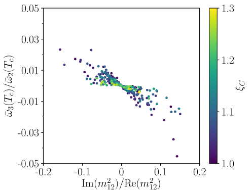
Figure 11: Type II, $H_{1}=h$: The value $\bar{\omega}_{3}(T_{c})/\bar{\omega}_{2}(T_{c})$ at the critical temperature $T_{c}$ versus $\mbox{Im}(m_{12}^{2})/\mbox{Re}(m_{12}^{2})\neq 0$ at $T=0$ for points with a strong PT. The colour code indicates the size of $\xi_{c}$.

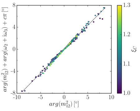
Figure 12: Type II, $H_{1}=h$: The total CP-violating angle at the critical temperature $T_{c}$ versus the CP-violating angle at $T=0$. By adding $c\pi$, $c\in\{-1,0,1\}$, the angle is ensured to lie in the range $-90^{\circ}$ to $90^{\circ}$. The colour code indicates the size of $\xi_{c}$.

Figure 11 shows the relation between $\tan\varphi^{\text{spont}}=\bar{\omega}_{3}(T_{c})/\bar{\omega}_{2}(T_{c})$ at the critical temperature $T_{c}$ and $\tan\varphi^{\text{explicit}}=\mbox{Im}(m_{12}^{2})/\mbox{Re}(m_{12}^{2})$ at vanishing temperature. All points comply with our constraints and feature a strong PT. Furthermore, only points with explicit CP violation are included, i.e. $\mbox{Im}(m_{12}^{2})/\mbox{Re}(m_{12}^{2})\neq 0$ although we allow it to be very small. The plot shows the correlation between the two types of CP-violating phases, with the absolute value of the spontaneously generated phase decreasing with increasing absolute value of the explicitly CP-violating phase. Like in the type I, we observe that the spontaneous generation of a CP-violating phase at the critical temperature only appears for scenarios with explicit CP violation at zero temperature. The color bar visualizes the size of $\xi_{c}$ at $T_{c}$. The maximum value attained in case of CP violation is somewhat smaller than in the type I case, with $\xi_{c}^{\text{max}}=1.3$. The smaller size of $\xi_{c}$ is to be attributed to the overall heavier mass spectrum in the type II model due to the lower bound on the charged Higgs mass. In the CP-violating case all Higgs bosons mix and hence the heavier Higgs bosons receive contributions from all VEVs, increasing their participation in the PT.

Figure 12 displays the total phase at $T_{c}$ as a function of the CP-violating angle at $T=0$. We see that the total phase varies between -7.6^∘ and +7.6^∘ and is hence much smaller than in type I. This is closely related to the fact that at zero temperature the applied constraints, mainly the EDM constraint, restrict a possible CP-violating phase at $T=0$ more strongly than in type I [87], namely to values between about -9^∘ and 8.6^∘. Due to the correlation between $\varphi^{\text{explicit}}$ and $\varphi^{\text{spont}}$ the total phase at $T_{c}$ is then smaller, so that in the type II C2HDM smaller CP-violating effects are to be expected from this mechanism.

9.2 Implications for LHC phenomenology

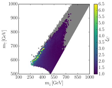
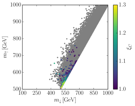
Figure 13: Type II, $H_{1}=h$: The mass of the heavier versus the lighter non-SM-like Higgs boson. Left: CP-conserving and CP-violating points, right: only CP-violating points. Grey: points passing all the constraints; color: points with additionally $\xi_{c}\geq 1$. The color code indicates the value of $\xi_{c}$.

Figure 13 shows the mass values of the neutral non-SM-like Higgs bosons compatible with all constraints (grey) that are additionally compatible with a strong PT (color), taking all points of the CP-conserving and CP-violating scenarios (left) and restricting to purely CP-violating scenarios (right). The results of Fig. 13 (left) basically agree with the results found in [51], taking into account the fact that the lower bound on $m_{H^{\pm}}$ has moved up to 580 GeV. Furthermore, we do not find valid points with $m_{\downarrow}<250$ GeV, which would come along with large mass gap of the heavier Higgs boson masses to $m_{\downarrow}$. Overall, grey points with mass gaps between $H_{\downarrow}$ and $H_{\uparrow}$ above 332 GeV are not allowed any more. This exclusion results from the unitarity check with the NLO Higgs self-couplings. The plot confirms that for the CP-conserving parameter points with $\xi_{c}^{\text{max}}=6.5$ larger $\xi_{c}$ values can be obtained than in the CP-violating case where $\xi_{c}^{\text{max}}=1.3$. The right plot shows that the inclusion of CP violation implies mass spectra where overall the non-SM-like Higgs masses move closer, cf. also Fig. 14. In particular most of the points with a strong PT feature $H_{\downarrow}$ and $H_{\uparrow}$ which are close in mass, and the largest $\xi_{c}$ values are found for the lightest possible values that they can have within the given constraints. Again this can easily be understood by reminding that due to CP violation all Higgs bosons mix and have a non-negligible VEV and that additionally in type II with $H_{1}\equiv h$ the non-SM-like neutral Higgs bosons are rather heavy. In order not to weaken the PT too much, in case of $H_{\uparrow}$ having a large portion of the VEV, it should be as light as possible and hence be mass degenerate with $H_{\downarrow}$, or in case it is not mass degenerate, the lighter of the two should acquire most of the VEV.

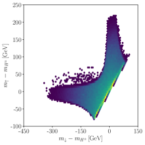
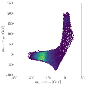
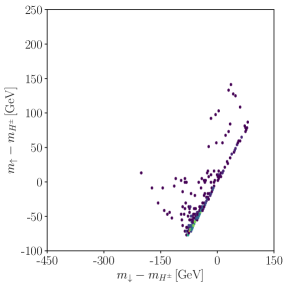
Figure 14: Type II, $H_{1}=h$: The mass difference $m_{\uparrow}-m_{H^{\pm}}$ versus $m_{\downarrow}-m_{H^{\pm}}$. The colour code shows the relative frequency of left: all points passing the constraints; middle: all points with a strong PT and CP conservation; right: all points with $\xi_{c}\geq 1$ and explicit CP violation.

The implications for LHC phenomenology can be read off Fig. 14, showing the mass differences of $H_{\uparrow}$ and $H^{\pm}$ versus the ones of $H_{\downarrow}$ and $H^{\pm}$. The colour code shows the relative frequency for all points passing the constraints (left), with additionally a strong PT and only CP-conserving points (middle) and for only CP-violating points with $\xi_{c}\geq 1$ (right). While the application of the constraints favours scenarios with degenerate neutral non-SM-like Higgs masses, the requirement of a strong PT favours a mass hierarchy between $m_{\uparrow}\approx m_{H^{\pm}}$ and $m_{\downarrow}$ with a mass gap of about 200 GeV. The comparison with the right plot shows that these are mostly CP-conserving scenarios. This allows for decays of $H_{\uparrow}\to ZH_{\downarrow}$ that can be searched for at the LHC. In contrast the right plot shows that the CP-violating case favors more degenerate masses of the non-SM-like Higgs bosons. This has consequences for LHC phenomenology. In order to quantify this we have chosen four exemplary benchmark scenarios featuring different mass patterns. We have one benchmark point, BP1T2, with almost degenerate $H_{\uparrow}$ and $H^{\pm}$ and a mass gap to the lighter $H_{\downarrow}$. In BP2T2, $H_{\downarrow}$ and $H^{\pm}$ are closer in mass and $H_{\uparrow}$ is the heaviest Higgs boson. The benchmarks BP3T2 and BP4T2 feature nearly mass degenerate $H_{\downarrow}$ and $H_{\uparrow}$ with a heavier charged Higgs boson in the former and a lighter one in the latter case. The input parameters are given in Table 10. The overall mass spectrum is heavier than in the type I C2HDM as expected from the lower bound on the charged Higgs mass in type II. The dominant branching are summarised in Table 11. These are determined by the mass pattern together with the fact that the $H_{3}VV$ ($V=W,Z$) coupling is very small despite $R_{33}^{2}$ being small in BP1T2-BP3T2. Besides the dominant decay into $t\bar{t}$, $H_{3}$ has a substantial branching ratio into $ZH_{2}$ in BP1T2 and in into $W^{\pm}H^{\mp}$ in BP2T2. In BP3T2 and BP4T2, the mass pattern forces $H_{3}$ to mainly decay into $t\bar{t}$. This is the dominant decay channel for $H_{2}$ in all four scenarios. The mass ordering of BP1T2 allows $H^{\pm}$ to decay with a significant branching ratio into $W^{\pm}H_{2}$ besides the dominant decay into $t\bar{b}$. For all the other scenarios $H^{\pm}$ almost exclusively decays into $t\bar{b}$. Again we find that the fact that in the C2HDM not only mass hierarchies with large mass gaps are preferred by the strong PT, induces also decay patterns with SM particles in the final state.

	BP1T2	BP2T2	BP3T2	BP4T2
$m_{H_{1}}$ [GeV]	125.09	125.09	125.09	125.09
$m_{H_{2}}$ [GeV]	436.834	652.592	551.699	695.347
$m_{H^{\pm}}$ [GeV]	640.079	616.659	629.564	614.739
$\mbox{Re}(m_{12}^{2})$ [GeV2]	85376	121817	73628	113941
$\alpha_{1}$	0.880	0.850	0.817	0.827
$\alpha_{2}$	-0.0156	$5.945\cdot 10^{-3}$	$3.687\cdot 10^{-3}$	-0.013
$\alpha_{3}$	1.568	-1.568	-1.557	0.085
$\tan\beta$	1.399	1.224	1.216	1.182
$m_{H_{3}}$ [GeV]	653.627	757.984	552.583	701.912
$\xi_{c}$	1.190	1.077	1.169	1.016
$R_{13}^{2}$	$2.437\cdot 10^{-4}$	$3.534\cdot 10^{-5}$	$1.360\cdot 10^{-7}$	$1.658\cdot 10^{-4}$
$R_{23}^{2}$	0.999	0.999	0.999	$7.144\cdot 10^{-3}$
$R_{33}^{2}$	$9.400\cdot 10^{-6}$	$7.433\cdot 10^{-6}$	$1.993\cdot 10^{-4}$	0.993
$\sigma_{hh}^{\text{NLO}}$ [fb]	62.16	38.97	57.15	42.78

Table 10: Line 1-8: The input parameters of the type II CP-violating benchmarks with $H_{1}\equiv h$ and $\xi_{c}>1$, compatible with all constraints. Line 9 to 13: The derived 3rd neutral Higgs boson mass, the $\xi_{c}$ value and the CP-odd admixtures $R_{i3}^{2}$. Line 14: The NLO QCD gluon fusion $hh$ production cross section at $\sqrt{s}=14$ TeV.

BP1T2	BP2T2	BP3T2/BP4T2
BR($H_{2}\to t\bar{t}$) = 0.98	BR($H_{2}\to t\bar{t}$) = 0.99	BR($H_{2}\to t\bar{t}$) = 0.97/0.98
BR($H_{3}\to t\bar{t}$) = 0.54	BR($H_{3}\to t\bar{t}$)=0.76	BR($H_{3}\to t\bar{t}$) = 0.97/0.98
BR($H_{3}\to ZH_{2}$) = 0.43	BR($H_{3}\to W^{\mp}H^{\pm}$)=0.22
BR($H^{+}\to t\bar{b}$) = 0.58	BR($H^{+}\to t\bar{b}$)=0.99	BR($H^{+}\to t\bar{b}$) = 0.98/0.99
BR($H^{\pm}\to WH_{2}$) = 0.40

Table 11: The dominant branching ratios of the BP1T2-BP4T2 Higgs bosons.

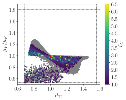
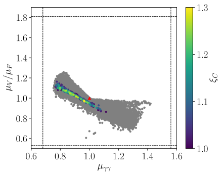
Figure 15: Type II, $H_{1}=h$: $\mu_{V}/\mu_{F}$ versus $\mu_{\gamma\gamma}$. Grey: all points passing the applied constraints, colour: all points with additionally $\xi_{c}\geq 1$; left: all 2HDM points, right: only C2HDM points. The red triangle marks the SM result.

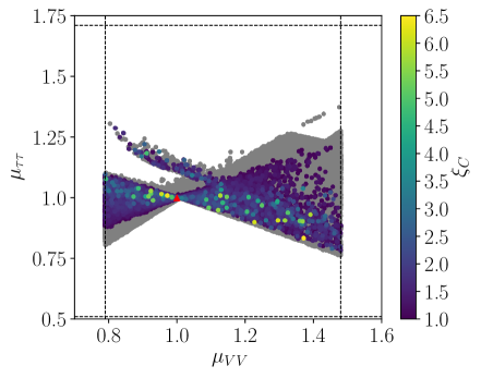
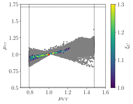
Figure 16: Type II, $H_{1}=h$: $\mu_{V}/\mu_{F}$ versus $\mu_{\gamma\gamma}$. Grey: all points passing the applied constraints, colour: all points with additionally $\xi_{c}\geq 1$; left: all 2HDM points, right: only C2HDM points. The red triangle marks the SM result.

In Fig. 15 we depict $\mu_{V}/\mu_{F}$ versus the photonic rate $\mu_{\gamma\gamma}$ in grey for all points passing the constraints and in colour for those with $\xi_{c}>1$. The left plot comprises all 2HDM points, while in the right plot only the CP-violating points are retained. The requirement of a strong PT restricts the region of allowed $\mu$ values, and the results of the left plot reconfirm our findings of [51] in the real 2HDM. Due to a more efficient scan procedure applied here, we have now more scenarios compatible with $\xi_{c}\geq 1$ in the wrong-sign limit region [134, 98, 135] (corresponding to the points in the lower left corner) where the $h$ coupling to the massive gauge bosons has an opposite sign with respect to its $b$-quark Yukawa coupling. The inclusion of CP violation restricts the $\mu$-values further. We see a strong correlation of $\mu_{\gamma\gamma}$ and $\mu_{V}/\mu_{F}$, with the latter decreasing with increasing $\mu_{\gamma\gamma}$. The wrong-sign limit is completely excluded which, however, is already almost excluded due to the applied constraints and not because of a strong PT. The CP-violating scenarios with $\xi_{c}\geq 1$ preclude $\mu_{V}/\mu_{F}$ above 1.17 and below 0.86 and $\mu_{\gamma\gamma}$ above 1.12 and below 0.76. Any values outside these ranges point to the CP-conserving 2HDM. Note also, that the SM point (red triangle) is not compatible with a strong PT in the C2HDM.

As can be inferred from Fig. 16, which is the same as Fig. 15 but for $\mu_{\tau\tau}$ versus $\mu_{VV}$, in the CP-violating case there is also a strong correlation between $\mu_{\tau\tau}$ and $\mu_{VV}$. The former increases with $\mu_{VV}$. Furthermore, no scenarios in the wrong-sign regime (corresponding to the points in the upper left corner of Fig. 16 (left)) are realized, which, again, is mostly due to the applied constraints. The value of $\mu_{\tau\tau}$ is restricted to values between 0.9 and 1.10, as well as $\mu_{VV}$ to the range between 0.8 and 1.22.

10 Analysis of the trilinear Higgs self-couplings and Higgs pair production in the C2HDM Type II

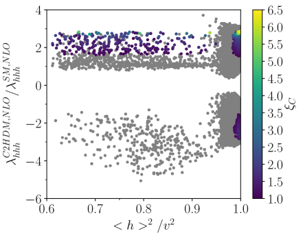
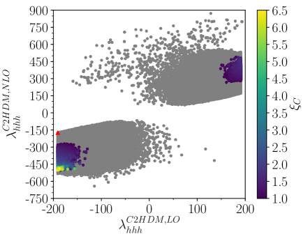
Figure 17: Type II, $H_{1}=h$: Left: the C2HDM trilinear Higgs self-coupling between three SM-like Higgs bosons $h$ normalized to the SM value, at NLO, as function of the fraction of the VEV squared carried by $h$; right: the NLO coupling versus the LO value. Grey: all points passing the constraints; colour: points with additionally $\xi_{c}>1$. The red triangle marks the SM point.

We conclude our investigation with the discussion of the interplay between the requirement of a strong PT and the trilinear Higgs self-coupling among the SM-like Higgs bosons. Figure 17 (left) depicts the values of the NLO trilinear Higgs coupling between three SM-like Higgs bosons $h$ of the C2HDM normalized to the SM value, each at NLO, as function of the fraction of the VEV squared carried by $h$, for all points passing the constraints (grey) and for only those with a strong PT (colour). As in the C2HDM type I, we observe that the C2HDM self-couplings can be enhanced with respect to the SM, with a maximum enhancement factor of 5.1. If additionally the PT is required to be of strong first order, the trilinear coupling has to be somewhat larger than in the SM, but must not be above a factor of about 2.9 the SM value, in order not to weaken the PT again due to too large Higgs masses. If only CP-violating points are taken into account this ratio is slightly lowered to 2.4. The right plot shows the NLO coupling versus the LO one and underlines the importance of the loop corrections. The wide spread points in the upper half of the plot and the two isolated points in the lower right part are due to the wrong-sign limit. In the regions with a strong PT the maximum corrections amount to about a factor 3.3, and the largest values of $\xi_{c}$ are found for the largest correction factor. Taking into account only the CP-violating scenarios, the maximum enhancement is lowered to 2.2. Note, that the sharp cut of the tree-level couplings at large values are due to tree-level unitarity. Interestingly, the plot shows that a vanishing trilinear Higgs self-coupling between the SM-like Higgs bosons is not compatible with the constraints any more, while in type I this was not excluded. Concerning the trilinear Higgs self-couplings also involving non-SM-like Higgs bosons we find the same overall features as in the type I case.

In Table 10 we give the NLO QCD $hh$ production cross sections through gluon fusion at $\sqrt{s}=14$ TeV for the four benchmark points BP1-4T2. The size of the non-SM-like Higgs boson masses allows for resonant enhancements through their on-shell production with subsequent decay into $hh$. Depending on the size of the Higgs self-couplings between them and $hh$, the C2HDM $hh$ cross section is more or less enhanced compared to the SM.

11 Conclusions

We have found that the NLO effects derived from the effective potential have a non-negligible influence on the global minimum and perturbativity at NLO. The requirement of the EW minimum to be the global minimum also at NLO excludes ${\cal O}(5-25\%)$ of the generated scenarios compatible with the applied constraints in the type I C2HDM with $H_{1}$ or $H_{2}\equiv h$, denoted by C2HDM(I${}_{H_{1}}$), and C2HDM(I${}_{H_{2}}$) and the type II C2HDM with $H_{1}\equiv h$, denoted by C2HDM(II${}_{H_{1}}$). In the type II C2HDM with $H_{2}\equiv h$, the mass differences enforced by the experimental constraints become large and, due to our renormalisation procedure, induce large corrections to the Higgs self-couplings so that a stable vacuum cannot be guaranteed any more so that we did not investigate this version of the C2HDM further in this paper. Along the same lines accordance with unitarity at NLO eliminates ${\cal O}(9-18\%)$ of the remaining points.

We showed that the presence of explicit CP violation at zero temperature induces spontaneous CP violation at the EWPT. The size of the induced phase correlates with the amount of explicit CP violation at $T=0$. In type I a larger CP-violating phase at zero temperature is compatible with the experimental constraints than in type II. Consequently, the total CP-violating angle, including the spontaneously generated CP-violating phase, at $T_{c}$ amounts up to 49^∘ in the C2HDM(I${}_{H_{1}}$) and up to about 8^∘ in the C2HDM(II${}_{H_{1}}$). In particular, in type I this should be large enough to ensure successful baryogenesis.

We overall re-confirm our findings of our previous investigation of the PT in the CP-conserving 2HDM for the scenarios in the CP-conserving limit. Deviations in type I occur due to an updated limit on $\tan\beta$ and in type II due to a more efficient scan procedure. A strong phase transition is found to be possible in all three different remaining set-ups including CP violation, i.e. the C2HDM(I${}_{H_{1,2}}$) and the C2HDM(II${}_{H_{1}}$). Overall, the strength of the phase transition is smaller in the CP-violating case, with $\xi_{c}^{\text{max}}=1.9$ in C2HDM(I${}_{H_{1}}$) and $\xi_{c}^{\text{max}}=1.3$ in C2HDM(II${}_{H_{1}}$). In C2HDM(I${}_{H_{2}}$) we find only three points (BPCPV1-3) that are compatible with a strong PT, with $\xi_{c}^{\text{max}}=1.48$. Although the SM-like Higgs boson has the largest fraction of the VEV at the PT and hence mainly drives its strength, through CP mixing all three neutral Higgs bosons, also the non-SM-ones, receive a VEV. Scenarios where heavy non-SM-like Higgs bosons receive a large portion of the VEV at the EWPT weaken its strength. Therefore either the lighter of the non-SM-like Higgs bosons receives the larger portion of the VEV among the two, or the overall spectrum is as light as possible.

	mass pattern	main phenomenological features
C2HDMI${}_{H_{1}}$	$m_{\phi}\equiv m_{\uparrow}\approx m_{H^{\pm}}$
BPi1	$m_{\phi}-m_{\downarrow}\approx 180$ GeV	BR${}^{\text{max}}$: $H_{\downarrow}\to hh$, $H_{\uparrow}\to ZH_{\downarrow}$, $H^{\pm}\to WH_{\downarrow}$
BPi2	$m_{\phi}-m_{\downarrow}\approx 260$ GeV	BR${}^{\text{max}}$: $H_{\downarrow}\to hh$, $H_{\uparrow}\to ZH_{\downarrow}$, $H^{\pm}\to WH_{\downarrow}$
		combination of $H_{2}$ decays into $hh$, $Zh$ and $WW$
		allow for test of CP-mixed nature of $H_{2}$
BPi3	$m_{\phi}-m_{\downarrow}\approx 300$ GeV	BR${}^{\text{max}}$: $H_{\downarrow}\to WW$ despite $R_{23}^{2}=0.7$
		$H_{\uparrow}\to ZH_{\downarrow}$, $H^{\pm}\to WH_{\downarrow}$
C2HDMI${}_{H_{1}}$	$m_{\varphi}\equiv m_{\downarrow}\approx m_{H^{\pm}}$
BPii1	$m_{\uparrow}-m_{\varphi}\approx 260$ GeV	BR${}^{\text{max}}$: $H_{\downarrow}\to WW$, $H_{\uparrow}\to W^{\mp}H^{\pm}$, $H^{+}\to t\bar{b}$
BPii2	$m_{\uparrow}-m_{\varphi}\approx 310$ GeV	BR${}^{\text{max}}$: as BPii1, $\varphi$ lighter
C2HDMI${}_{H_{1}}$	$m_{0}\equiv m_{\downarrow}\approx m_{\uparrow}$
BPiii1	$m_{0}-m_{H^{\pm}}\approx 0$ GeV	BR${}^{\text{max}}$: $H_{\downarrow,\uparrow}\to t\bar{t}$, $H^{+}\to t\bar{b}$
BPiii2	$m_{H^{\pm}}-m_{0}\approx 80$ GeV	BR${}^{\text{max}}$: as BPiii1
BPiii3	$m_{0}-m_{H^{\pm}}\approx 77$ GeV	BR${}^{\text{max}}$: as BPiii1
C2HDMI${}_{H_{2}}$	overall lighter spectrum than in C2HDMI${}_{H_{1}}$
BPCPV1	$m_{H_{3}}\approx m_{H^{\pm}}\approx 375$ GeV	$H_{\downarrow}$ ($H_{\uparrow}$) mostly CP-even (CP-odd)
	$m_{\downarrow}=120$ GeV	BR${}^{\text{max}}$: $H_{\downarrow}\to b\bar{b}$, $H_{\uparrow}\to ZH_{\downarrow}$, $H^{\pm}\to W^{\pm}H_{\downarrow}$
BPCPV2	max. mass $m_{H^{\pm}}=192$ GeV	$H_{\downarrow}$, $H_{\uparrow}$ CP-mixed
	$m_{\downarrow}=91$ GeV	BR${}^{\text{max}}$: $H_{\downarrow}\to b\bar{b}$, $H_{\uparrow}\to WW$, $H^{\pm}\to W^{\pm}H_{\downarrow}$
BPCPV3	max. mass $m_{H^{\pm}}=167$ GeV	$H_{\downarrow}$ ($H_{\uparrow}$) mostly CP-odd (CP-even)
	$m_{\downarrow}=118$ GeV	BR${}^{\text{max}}$: $H_{\downarrow}\to b\bar{b}$, $H_{\uparrow}\to WW$, $H^{\pm}\to W^{\pm}H_{\downarrow}$
C2HDMII${}_{H_{1}}$	overall heavier spectrum than in C2HDM(I)
BP1T2	$m_{\downarrow}=437$ GeV	BR${}^{\text{max}}:$ BR$(H_{\downarrow}\to t\bar{t})$ = 0.98
	$m_{H^{\pm}}=640$, $m_{\uparrow}=654$ GeV	BR$(H_{3}\to t\bar{t}/ZH_{\downarrow})$ = 0.54/0.43,
		BR$(H^{\pm}\to t\bar{b}/WH_{\downarrow})$ = 0.58/0.40
BP2T2	$m_{H^{\pm}}=617$, $m_{\downarrow}=653$ GeV	BR${}^{\text{max}}:$ BR$(H_{\downarrow}\to t\bar{t})$ = 0.99
	$m_{\uparrow}=758$ GeV	BR$(H_{3}\to t\bar{t}/W^{\pm}H^{\mp})$ = 0.76/0.22,
		BR$(H^{+}\to t\bar{b})$ = 0.99
BP3T2	$m_{\downarrow}\approx m_{\uparrow}\approx 552$ GeV	BR${}^{\text{max}}$ all almost exclusively:
	$m_{H^{\pm}}=630$ GeV	$H_{\downarrow}\to t\bar{t}$, $H_{\uparrow}\to t\bar{t}$, $H^{+}\to t\bar{b}$
BP4T2	$m_{H^{\pm}}=615$ GeV	BR${}^{\text{max}}$ all almost exclusively:
	$m_{\downarrow}\approx m_{\uparrow}\approx 698$ GeV	$H_{\downarrow}\to t\bar{t}$, $H_{\uparrow}\to t\bar{t}$, $H^{+}\to t\bar{b}$

Table 12: Main features of the CP-violating benchmark points with a strong phase transition.

Concerning the mass hierarchies and hence the implications for phenomenology, we confirm for scenarios compatible with a strong PT in the CP-conserving limit the preference for a mass hierarchy with a gap between the heavier and the lighter neutral non-SM-like Higgs bosons. The heavier Higgs boson therefore mainly decays into gauge+Higgs final states. Depending on the value of the charged Higgs mass, which due to electroweak precision physics constraints has to be mass degenerate with one of the neutral Higgs bosons, these final state particles are neutral $(ZH_{i})$ or charged $(W^{\pm}H^{\mp})$. Such decays are a clear indication of non-SM physics arising from an enlarged Higgs sector, which can be searched for at the LHC. For CP-violating scenarios, however, no such preference is found: The requirement of a strong phase transition combined with a CP-violating set-up where all Higgs bosons receive a VEV, besides this mass pattern, also favours scenarios where all three neutral Higgs bosons are rather close in mass. There are scenarios with one or two of the non-SM-like neutral Higgs bosons degenerate with the charged Higgs boson. Without mass hierarchies between the non-SM-like Higgs bosons (and small gauge-Higgs pair couplings involving the $h$) they all decay into SM final states, with the specific nature of the final state particles determined by the mass of the decaying Higgs boson. Among the scenarios with a mass hierarchy we also have Higgs-to-Higgs decays and decay patterns that allow to identify the CP-violating nature of the Higgs boson through the combination of its decay channels. We have provided several benchmark scenarios for the C2HDM with a strong PT. Their key features are summarised in Table 12.

The $\mu$-values of the SM-like Higgs boson in the C2HDM with a strong PT turn out to be more restricted than in the CP-conserving case. This can be exploited to exclude the C2HDM and additionally distinguish it from the 2HDM. We summarise the distinctive features of the $\mu$-values in Table 13. The regions are excluded by the C2HDM but not by the 2HDM. Any measured value outside these regions rules out the CP-violating set-up for successful baryogenesis. Note, however, that the wrong-sign-limit is mainly disfavoured by the applied constraints and not by the requirement of $\xi_{c}>1$ in contrast to the other regions given in the Table.

excluded	$\mu_{V}/\mu_{F}-\mu_{\gamma\gamma}$	$\mu_{\tau\tau}-\mu_{VV}$
C2HDM(I${}_{H_{1}}$)	$\mu_{V}/\mu_{F}<0.9$ and $\mu_{\gamma\gamma}<0.9$	$\mu_{\tau\tau}>1$ and $\mu_{VV}<1$
C2HDM(II${}_{H_{1}}$)	$\mu_{\gamma\gamma}>1.12$	$\mu_{VV}>1.22$
	$\mu_{\gamma\gamma}<1$ and $\mu_{V}/\mu_{F}<0.82$ (wsl)	$\mu_{VV}<1.13$ and $\mu_{\tau\tau}>1.07$ (wsl)
	$\mu_{V}/\mu_{F}=\mu_{\gamma\gamma}=1$ (SM point)

Table 13: Distinguishing features between the C2HDM and 2HDM rates for scenarios with $\xi_{c}>1$: The C2HDM excluded regions given here are still allowed by the 2HDM. Note that the wrong-sign limit (wsl) regions are excluded due to the applied constraints and not due to $\xi_{c}>1$.

From the loop-corrected effective potential we derive the NLO-corrected effective trilinear Higgs couplings. The C2HDM couplings can be enhanced or suppressed relative to the SM case for all scenarios compatible with the experimental and theoretical constraints. (Note, that the maximum allowed value is constrained by the requirement of unitarity.) The scenarios with a strong PT, however, require enhanced trilinear Higgs self-couplings between the SM-like Higgs bosons, which is the Higgs boson with the largest VEV and hence mainly drives the phase transition. Including also the points in the CP-conserving limit, the two enhancement regions are $\lambda_{hhh}^{\text{C2HDM,NLO}}/\lambda_{hhh}^{\text{NLO,SM}}=$ (-2.73…-1.1) and (1.1…2.9) for C2HDM(I${}_{H_{1}}$), (-2.32…-0.94) and (1.04…2.58) for C2HDM(I${}_{H_{2}}$) and (-2.83…-1.54) and (1.55…2.93) for C2HDM(II${}_{H_{1}}$). For the purely CP-violating points these values reduce to (-2.30…-1.28) and (1.26…2.46) for C2HDM(I${}_{H_{1}}$), -1.03 and (1.03…1.54) for C2HDM(I${}_{H_{2}}$) and (-2.35…-1.65) and (1.64…2.36) for C2HDM(II${}_{H_{1}}$). Some of these deviations are large enough to be measurable at the LHC. Note, that the upper bound on the coupling comes from the requirement not to weaken the PT again through too heavy Higgs masses. The NLO corrections are important, changing the LO coupling by up to a factor (1.07…8.25) in C2HDM(I${}_{H_{1}}$), a factor (0.93…2.32) in C2HDM(I${}_{H_{2}}$) and (1.46…3.31) in C2HDM(II${}_{H_{1}}$), for the scenarios compatible with $\xi_{c}>1$. Concentrating on purely CP-violating points these factors change to (1.31…2.44), (0.93…1.35) and (1.51…2.17), respectively. The investigation of the trilinear self-couplings involving the non-SM-like Higgs bosons shows that the C2HDM values can be enhanced or suppressed compared to the SM, that the enhancement is less important for scenarios with a strong PT and that the NLO corrections are significant. We summarise that the requirement of a strong PT induces enhanced trilinear Higgs self-couplings among the SM-like Higgs bosons that deviate from the SM value significantly enough to be measurable at the LHC. The experimental confirmation of large self-couplings establishes a clear connection between a strong PT, i.e. cosmology, and collider physics. The self-coupling is extracted from Higgs pair production at the LHC, with the main channel given by gluon fusion. We calculated for our benchmark scenarios the cross sections for $hh$ production including the NLO QCD corrections in the large top quark mass limit. Due to the possible resonant production of heavy Higgs bosons with subsequent decay into $hh$ they are all enhanced compared to the SM case, so that the prospects for measuring them are promising. These cross sections do not include EW corrections, as they are not available. The derived sizes of the EW-corrected effective Higgs self-couplings indicate that these corrections can be sizeable. They could lower the Higgs pair production cross section.

In conclusion, the requirement of a strong PT with successful baryogenesis demands an enlarged Higgs sector and has measurable consequences for the C2HDM. In contrast to the real 2HDM not only mass gaps between the Higgs bosons, but also degenerate scenarios are favoured. The C2HDM with a strong PT predicts strong correlations among the signal strengths of the SM-like Higgs boson. Finally, the trilinear $hhh$ coupling must be enhanced compared to the SM, and the additional Higgs bosons induce $hh$ production cross sections that are larger than in the SM case and can be measured at the LHC. The combination of successful baryogenesis with collider phenomenology is a powerful tool to further restrict the underlying model and to identify its true nature.

References

- [1] G. Aad et al. [ATLAS Collaboration], Phys. Lett. B 716 (2012) 1 [arXiv:1207.7214 [hep-ex]]; G. Aad et al. [ATLAS Collaboration], ATLAS-CONF-2012-162.
- [2] S. Chatrchyan et al. [CMS Collaboration], Phys. Lett. B 716 (2012) 30 [arXiv:1207.7235 [hep-ex]]; S. Chatrchyan et al. [CMS Collaboration], CMS-PAS-HIG-12-045.
- [3] G. Aad et al. [ATLAS Collaboration], Eur. Phys. J. C 75 (2015) 10, 476 [arXiv:1506.05669 [hep-ex]].
- [4] V. Khachatryan et al. [CMS Collaboration], Phys. Rev. D 92 (2015) 1, 012004 [arXiv:1411.3441 [hep-ex]].
- [5] G. Aad et al. [ATLAS Collaboration], Eur. Phys. J. C 76 (2016) no.1, 6 [arXiv:1507.04548 [hep-ex]].
- [6] V. Khachatryan et al. [CMS Collaboration], Eur. Phys. J. C 75 (2015) 5, 212 [arXiv:1412.8662 [hep-ex]].
- [7] C. L. Bennett et al. [WMAP Collaboration], Astrophys. J. Suppl. 208 (2013) 20 [arXiv:1212.5225 [astro-ph.CO]].
- [8] V. A. Kuzmin, V. A. Rubakov and M. E. Shaposhnikov, Phys. Lett. B 155 (1985) 36.
- [9] A. G. Cohen, D. B. Kaplan and A. E. Nelson, Nucl. Phys. B 349 (1991) 727.
- [10] A. G. Cohen, D. B. Kaplan and A. E. Nelson, Ann. Rev. Nucl. Part. Sci. 43 (1993) 27 [hep-ph/9302210].
- [11] M. Quiros, Helv. Phys. Acta 67 (1994) 451.
- [12] V. A. Rubakov and M. E. Shaposhnikov, Usp. Fiz. Nauk 166 (1996) 493 [Phys. Usp. 39 (1996) 461] [hep-ph/9603208].
- [13] K. Funakubo, Prog. Theor. Phys. 96 (1996) 475 [hep-ph/9608358].
- [14] M. Trodden, Rev. Mod. Phys. 71 (1999) 1463 [hep-ph/9803479].
- [15] W. Bernreuther, Lect. Notes Phys. 591 (2002) 237 [hep-ph/0205279].
- [16] D. E. Morrissey and M. J. Ramsey-Musolf, New J. Phys. 14 (2012) 125003 [arXiv:1206.2942 [hep-ph]].
- [17] A.D. Sakharov, ZhETF Pis’ma 5 (1967) 32 (JETP Letters 5 (1967) 24).
- [18] N. S. Manton, Phys. Rev. D 28 (1983) 2019.
- [19] F. R. Klinkhamer and N. S. Manton, Phys. Rev. D 30 (1984) 2212.
- [20] C. Grojean and G. Servant, Phys. Rev. D 75 (2007) 043507 [hep-ph/0607107].
- [21] C. Caprini et al., JCAP 1604 (2016) no.04, 001 [arXiv:1512.06239 [astro-ph.CO]].
- [22] M. Hindmarsh, S. J. Huber, K. Rummukainen and D. J. Weir, Phys. Rev. D 92 (2015) no.12, 123009 [arXiv:1504.03291 [astro-ph.CO]].
- [23] S. J. Huber, T. Konstandin, G. Nardini and I. Rues, JCAP 1603 (2016) no.03, 036 [arXiv:1512.06357 [hep-ph]].
- [24] K. Hashino, M. Kakizaki, S. Kanemura and T. Matsui, Phys. Rev. D 94 (2016) no.1, 015005 [arXiv:1604.02069 [hep-ph]].
- [25] A. Addazi, Mod. Phys. Lett. A 32 (2017) no.08, 1750049 [arXiv:1607.08057 [hep-ph]].
- [26] P. Huang, A. J. Long and L. T. Wang, Phys. Rev. D 94 (2016) no.7, 075008 [arXiv:1608.06619 [hep-ph]].
- [27] K. Hashino, M. Kakizaki, S. Kanemura, P. Ko and T. Matsui, Phys. Lett. B 766 (2017) 49 [arXiv:1609.00297 [hep-ph]].
- [28] V. Vaskonen, arXiv:1611.02073 [hep-ph].
- [29] G. C. Dorsch, S. J. Huber, T. Konstandin and J. M. No, JCAP 1705 (2017) no.05, 052 [arXiv:1611.05874 [hep-ph]].
- [30] M. Saeedhosini and A. Tofighi, Adv. High Energy Phys. 2017 (2017) 7638204 [arXiv:1701.02074 [hep-ph]].
- [31] W. Chao, H. K. Guo and J. Shu, arXiv:1702.02698 [hep-ph].
- [32] L. Marzola, A. Racioppi and V. Vaskonen, arXiv:1704.01034 [hep-ph].
- [33] L. Bian, H. K. Guo and J. Shu, arXiv:1704.02488 [hep-ph].
- [34] M. Hindmarsh, S. J. Huber, K. Rummukainen and D. J. Weir, arXiv:1704.05871 [astro-ph.CO].
- [35] D. J. Weir, arXiv:1705.01783 [hep-ph].
- [36] Z. Kang, P. Ko and T. Matsui, arXiv:1706.09721 [hep-ph].
- [37] R. G. Cai, M. Sasaki and S. J. Wang, JCAP 1708 (2017) no.08, 004 [arXiv:1707.03001 [astro-ph.CO]].
- [38] C. W. Chiang and E. Senaha, arXiv:1707.06765 [hep-ph].
- [39] R. Jinno, S. Lee, H. Seong and M. Takimoto, arXiv:1708.01253 [hep-ph].
- [40] F. P. Huang and C. S. Li, arXiv:1709.09691 [hep-ph].
- [41] K. Kajantie, K. Rummukainen and M. E. Shaposhnikov, Nucl. Phys. B 407 (1993) 356 [hep-ph/9305345]; Z. Fodor, J. Hein, K. Jansen, A. Jaster and I. Montvay, Nucl. Phys. B 439 (1995) 147 [hep-lat/9409017]; K. Kajantie, M. Laine, K. Rummukainen and M. E. Shaposhnikov, Nucl. Phys. B 466 (1996) 189 [hep-lat/9510020]; K. Jansen, Nucl. Phys. Proc. Suppl. 47 (1996) 196 [hep-lat/9509018].
- [42] K. Kajantie, M. Laine, K. Rummukainen and M. E. Shaposhnikov, Phys. Rev. Lett. 77 (1996) 2887 [hep-ph/9605288]; F. Csikor, Z. Fodor and J. Heitger, Phys. Rev. Lett. 82 (1999) 21 [hep-ph/9809291].
- [43] M. B. Gavela, P. Hernandez, J. Orloff and O. Pene, Mod. Phys. Lett. A 9 (1994) 795 [hep-ph/9312215].
- [44] T. Konstandin, Phys. Usp. 56 (2013) 747 [Usp. Fiz. Nauk 183 (2013) 785] [arXiv:1302.6713 [hep-ph]].
- [45] J. M. Cline, hep-ph/0609145.
- [46] T. D. Lee, Phys. Rev. D 8 (1973) 1226.
- [47] G. C. Branco, P. M. Ferreira, L. Lavoura, M. N. Rebelo, M. Sher and J. P. Silva, Phys. Rept. 516 (2012) 1 [arXiv:1106.0034 [hep-ph]].
- [48] A. I. Bochkarev, S. V. Kuzmin and M. E. Shaposhnikov, Phys. Lett. B 244 (1990) 275; L. D. McLerran, M. E. Shaposhnikov, N. Turok and M. B. Voloshin, Phys. Lett. B 256 (1991) 451; A. I. Bochkarev, S. V. Kuzmin and M. E. Shaposhnikov, Phys. Rev. D 43 (1991) 369; N. Turok and J. Zadrozny, Nucl. Phys. B 358, 471 (1991); A. G. Cohen, D. B. Kaplan and A. E. Nelson, Phys. Lett. B 263 (1991) 86; N. Turok and J. Zadrozny, Nucl. Phys. B 369 (1992) 729; A. E. Nelson, D. B. Kaplan and A. G. Cohen, Nucl. Phys. B 373 (1992) 453; K. Funakubo, A. Kakuto and K. Takenaga, Prog. Theor. Phys. 91 (1994) 341; A. T. Davies, C. D. froggatt, G. Jenkins and R. G. Moorhouse, Phys. Lett. B 336 (1994) 464; J. M. Cline, K. Kainulainen and A. P. Vischer, Phys. Rev. D 54 (1996) 2451.
- [49] G. C. Dorsch, S. J. Huber and J. M. No, JHEP 1310 (2013) 029 [arXiv:1305.6610 [hep-ph]].
- [50] G. C. Dorsch, S. J. Huber, K. Mimasu and J. M. No, Phys. Rev. Lett. 113 (2014) no.21, 211802 [arXiv:1405.5537 [hep-ph]].
- [51] P. Basler, M. Krause, M. Muhlleitner, J. Wittbrodt and A. Wlotzka, JHEP 1702 (2017) 121 [arXiv:1612.04086 [hep-ph]].
- [52] G. C. Dorsch, S. J. Huber, K. Mimasu and J. M. No, arXiv:1705.09186 [hep-ph].
- [53] K. Funakubo, A. Kakuto, S. Otsuki, K. Takenaga and F. Toyoda, Prog. Theor. Phys. 94 (1995) 845.
- [54] J. M. Cline, K. Kainulainen and A. P. Vischer, Phys. Rev. D 54 (1996) 2451 [hep-ph/9506284].
- [55] K. Funakubo, A. Kakuto, S. Otsuki and F. Toyoda, Prog. Theor. Phys. 96 (1996) 771.
- [56] J. M. Cline and P. A. Lemieux, Phys. Rev. D 55 (1997) 3873 [hep-ph/9609240].
- [57] L. Fromme, S. J. Huber and M. Seniuch, JHEP 0611 (2006) 038.
- [58] J. M. Cline, K. Kainulainen and M. Trott, JHEP 1111 (2011) 089 [arXiv:1107.3559 [hep-ph]].
- [59] A. Haarr, A. Kvellestad and T. C. Petersen, arXiv:1611.05757 [hep-ph].
- [60] I. F. Ginzburg, M. Krawczyk and P. Osland, In *Seogwipo 2002, Linear colliders* 90-94 [hep-ph/0211371].
- [61] S. Inoue, M. J. Ramsey-Musolf, and Y. Zhang, Phys. Rev. D89, 115023 (2014), 1403.4257.
- [62] ACME, J. Baron et al., Science 343, 269 (2014), 1310.7534.
- [63] A. Ayala, L. A. Hernández and J. Salinas, Phys. Rev. D 95 (2017) no.12, 123004 [arXiv:1704.05510 [hep-ph]].
- [64] W. Chao, arXiv:1706.01041 [hep-ph].
- [65] S. Bruggisser, T. Konstandin and G. Servant, arXiv:1706.08534 [hep-ph].
- [66] T. Huang, J. M. No, L. Pernié, M. Ramsey-Musolf, A. Safonov, M. Spannowsky and P. Winslow, Phys. Rev. D 96 (2017) no.3, 035007 [arXiv:1701.04442 [hep-ph]].
- [67] B. Jain, S. J. Lee and M. Son, arXiv:1709.03232 [hep-ph].
- [68] M. Reichert, A. Eichhorn, H. Gies, J. M. Pawlowski, T. Plehn and M. M. Scherer, arXiv:1711.00019 [hep-ph].
- [69] S. Coleman and E. Weinberg, Phys. Rev. D 7 (1973) 1888.
- [70] L. Dolan and R. Jackiw, Phys. Rev. D 9 (1974) 3320.
- [71] M. Quiros, hep-ph/9901312.
- [72] M. E. Carrington, Phys. Rev. D 45 (1992) 2933.
- [73] G. D. Moore, Phys. Rev. D 59 (1999) 014503.
- [74] H. H. Patel and M. J. Ramsey-Musolf, JHEP 1107 (2011) 029 [arXiv:1101.4665 [hep-ph]].
- [75] C. Wainwright, S. Profumo and M. J. Ramsey-Musolf, Phys. Rev. D 84 (2011) 023521 [arXiv:1104.5487 [hep-ph]].
- [76] M. Garny and T. Konstandin, JHEP 1207 (2012) 189 [arXiv:1205.3392 [hep-ph]].
- [77] D. Land and E. D. Carlson, Phys. Lett. B 292 (1992) 107 [hep-ph/9208227].
- [78] A. Hammerschmitt, J. Kripfganz and M. G. Schmidt, Z. Phys. C 64 (1994) 105 [hep-ph/9404272].
- [79] D. Fontes, J. C. Romao, and J. P. Silva, JHEP 12, 043 (2014), 1408.2534
- [80] P. M. Ferreira, R. Santos and A. Barroso, Phys. Lett. B 603 (2004) 219 Erratum: [Phys. Lett. B 629 (2005) 114] [hep-ph/0406231].
- [81] A. Barroso, P. M. Ferreira and R. Santos, Phys. Lett. B 652 (2007) 181 [hep-ph/0702098 [HEP-PH]].
- [82] I. P. Ivanov, Phys. Rev. D 77 (2008) 015017 [arXiv:0710.3490 [hep-ph]].
- [83] P. M. Ferreira and B. Swiezewska, JHEP 1604 (2016) 099 [arXiv:1511.02879 [hep-ph]].
- [84] A. W. El Kaffas, P. Osland and O. M. Ogreid, Nonlin. Phenom. Complex Syst. 10 (2007) 347 [hep-ph/0702097 [hep-ph]].
- [85] W. Khater and P. Osland, Nucl. Phys. B661, 209 (2003), hep-ph/0302004.
- [86] D. Fontes, J. C. Romao, R. Santos and J. P. Silva, JHEP 1506 (2015) 060 [arXiv:1502.01720 [hep-ph]].
- [87] M. Muhlleitner, M. O. P. Sampaio, R. Santos and J. Wittbrodt, JHEP 1708 (2017) 132 [arXiv:1703.07750 [hep-ph]].
- [88] R. Grober, M. Muhlleitner and M. Spira, arXiv:1705.05314 [hep-ph].
- [89] M. Carena, G. Nardini, M. Quiros and C. E. M. Wagner, Nucl. Phys. B 812 (2009) 243 [arXiv:0809.3760 [hep-ph]].
- [90] P. B. Arnold and O. Espinosa, Phys. Rev. D 47 (1993) 3546 Erratum: [Phys. Rev. D 50 (1994) 6662] [hep-ph/9212235].
- [91] R. R. Parwani, Phys. Rev. D 45 (1992) 4695 Erratum: [Phys. Rev. D 48 (1993) 5965].
- [92] E. J. Weinberg and A. Wu, Phys. Rev. D 36 (1987) 2474.
- [93] J. E. Camargo-Molina, A. P. Morais, R. Pasechnik, M. O. P. Sampaio and J. Wessén, JHEP 1608 (2016) 073 [arXiv:1606.07069 [hep-ph]].
- [94] S. P. Martin, Phys. Rev. D 90 (2014) no.1, 016013 [arXiv:1406.2355 [hep-ph]].
- [95] J. Elias-Miro, J. R. Espinosa and T. Konstandin, JHEP 1408 (2014) 034 [arXiv:1406.2652 [hep-ph]].
- [96] J. A. Casas, J. R. Espinosa, M. Quiros and A. Riotto, Nucl. Phys. B 436 (1995) 3 Erratum: [Nucl. Phys. B 439 (1995) 466] [hep-ph/9407389].
- [97] R. Coimbra, M. O. P. Sampaio and R. Santos, Eur. Phys. J. C 73 (2013) 2428 [arXiv:1301.2599 [hep-ph]].
- [98] P. M. Ferreira, R. Guedes, M. O. P. Sampaio and R. Santos, JHEP 1412 (2014) 067 [arXiv:1409.6723 [hep-ph]].
- [99] I. P. Ivanov and J. P. Silva, Phys. Rev. D92, 055017 (2015), 1507.05100.
- [100] H. E. Haber and H. E. Logan, Phys. Rev. D 62 (2000) 015011 [hep-ph/9909335].
- [101] O. Deschamps, S. Descotes-Genon, S. Monteil, V. Niess, S. T’Jampens and V. Tisserand, Phys. Rev. D 82 (2010) 073012 [arXiv:0907.5135 [hep-ph]].
- [102] F. Mahmoudi and O. Stal, Phys. Rev. D 81 (2010) 035016 [arXiv:0907.1791 [hep-ph]].
- [103] T. Hermann, M. Misiak and M. Steinhauser, JHEP 1211 (2012) 036 [arXiv:1208.2788 [hep-ph]].
- [104] M. Misiak et al., Phys. Rev. Lett. 114 (2015) no.22, 221801 [arXiv:1503.01789 [hep-ph]].
- [105] M. Misiak and M. Steinhauser, Eur. Phys. J. C 77 (2017) no.3, 201 [arXiv:1702.04571 [hep-ph]].
- [106] M. Baak et al. [Gfitter Group Collaboration], Eur. Phys. J. C 74 (2014) 3046 [arXiv:1407.3792 [hep-ph]].
- [107] G. Aad et al. [ATLAS and CMS Collaborations], Phys. Rev. Lett. 114 (2015) 191803 [arXiv:1503.07589 [hep-ex]].
- [108] P. Bechtle, O. Brein, S. Heinemeyer, G. Weiglein and K. E. Williams, Comput. Phys. Commun. 181 (2010) 138 [arXiv:0811.4169 [hep-ph]]; P. Bechtle, O. Brein, S. Heinemeyer, G. Weiglein and K. E. Williams, Comput. Phys. Commun. 182 (2011) 2605 [arXiv:1102.1898 [hep-ph]]; P. Bechtle, O. Brein, S. Heinemeyer, O. Stål, T. Stefaniak, G. Weiglein and K. E. Williams, Eur. Phys. J. C 74 (2014) no.3, 2693 [arXiv:1311.0055 [hep-ph]].
- [109] G. Aad et al. [ATLAS and CMS Collaborations], JHEP 1608 (2016) 045 [arXiv:1606.02266 [hep-ex]].
- [110] A. Djouadi, J. Kalinowski, and M. Spira, Comput. Phys. Commun. 108, 56 (1998), hep-ph/9704448.
- [111] J. M. Butterworth et al., THE TOOLS AND MONTE CARLO WORKING GROUP Summary Report from the Les Houches 2009 Workshop on TeV Colliders, in Physics at TeV colliders. Proceedings, 6th Workshop, dedicated to Thomas Binoth, Les Houches, France, June 8-26, 2009, 2010, [arXiv:1003.1643 [hep-ph]].
- [112] T. Abe, J. Hisano, T. Kitahara, and K. Tobioka, JHEP 01, 106 (2014), 1311.4704, [Erratum: JHEP04,161(2016)].
- [113] K. A. Olive et al. [Particle Data Group Collaboration], Chin. Phys. C 38 (2014) 090001.
- [114] A. Denner et al., LHCHXSWG-INT-2015-006, url: https://cds.cern.ch/record/2047636.
-
[115]
LHC Higgs Cross SectionWorking Group,
https://twiki.cern.ch/twiki/bin/view/LHCPhysics/LHCHXSWG . - [116] S. Dittmaier et al. [LHC Higgs Cross Section Working Group Collaboration], arXiv:1101.0593 [hep-ph].
- [117] J. Baglio, O. Eberhardt, U. Nierste and M. Wiebusch, Phys. Rev. D 90 (2014) no.1, 015008 [arXiv:1403.1264 [hep-ph]].
- [118] B. Hespel, D. Lopez-Val and E. Vryonidou, JHEP 1409 (2014) 124 [arXiv:1407.0281 [hep-ph]].
- [119] J. F. Gunion and H. E. Haber, Phys. Rev. D 67 (2003) 075019 [hep-ph/0207010].
-
[120]
The Gfitter Collaboration, talk at EPS 2016,
https://indico.cern.ch/event/466934/contributions/2575352/. - [121] S. Dawson, S. Dittmaier and M. Spira, Phys. Rev. D 58 (1998) 115012 [hep-ph/9805244].
- [122] G. C. Branco, L. Lavoura and J. P. Silva, Int. Ser. Monogr. Phys. 103 (1999) 1.
- [123] D. Fontes, J. C. Romão, R. Santos and J. P. Silva, Phys. Rev. D 92 (2015) no.5, 055014 [arXiv:1506.06755 [hep-ph]].
- [124] S. F. King, M. Muhlleitner, R. Nevzorov and K. Walz, Nucl. Phys. B 901 (2015) 526 [arXiv:1508.03255 [hep-ph]].
- [125] S. Kanemura, S. Kiyoura, Y. Okada, E. Senaha and C. P. Yuan, Phys. Lett. B 558 (2003) 157, [hep-ph/0211308].
- [126] J. Baglio, A. Djouadi, R. Grober, M. M. Muhlleitner, J. Quevillon and M. Spira, JHEP 1304 (2013) 151, [arXiv:1212.5581 [hep-ph]].
- [127] M. Krause, M. Muhlleitner, R. Santos and H. Ziesche, Phys. Rev. D95 (2017) no.7, 075019 [arXiv:1609.04185 [hep-ph]].
- [128] E. W. N. Glover and J. J. van der Bij, Nucl. Phys. B309, 282 (1988).
- [129] T. Plehn, M. Spira, and P. M. Zerwas, Nucl. Phys. B479, 46 (1996), hep-ph/9603205, [Erratum: Nucl. Phys. B531, 655 (1998)].
- [130] See M. Spira’s website http://tiger.web.psi.ch/proglist.html.
- [131] S. Borowka, N. Greiner, G. Heinrich, S. P. Jones, M. Kerner, J. Schlenk, U. Schubert and T. Zirke, Phys. Rev. Lett. 117 (2016) no.1, 012001 Erratum: [Phys. Rev. Lett. 117 (2016) no.7, 079901] [arXiv:1604.06447 [hep-ph]].
- [132] S. Borowka, N. Greiner, G. Heinrich, S. P. Jones, M. Kerner, J. Schlenk and T. Zirke, JHEP 1610 (2016) 107 [arXiv:1608.04798 [hep-ph]].
- [133] G. Heinrich, S. P. Jones, M. Kerner, G. Luisoni and E. Vryonidou, JHEP 1708 (2017) 088 [arXiv:1703.09252 [hep-ph]].
- [134] P. M. Ferreira, J. F. Gunion, H. E. Haber and R. Santos, Phys. Rev. D 89 (2014) no.11, 115003 [arXiv:1403.4736 [hep-ph]].
- [135] D. Fontes, J. C. Romao and J. P. Silva, Phys. Rev. D 90 (2014) no.1, 015021 [arXiv:1406.6080 [hep-ph]].