A GPU Poisson-Fermi Solver for Ion Channel Simulations

Abstract. The Poisson-Fermi model is an extension of the classical Poisson-Boltzmann model to include the steric and correlation effects of ions and water treated as nonuniform spheres in aqueous solutions. Poisson-Boltzmann electrostatic calculations are essential but computationally very demanding for molecular dynamics or continuum simulations of complex systems in molecular biophysics and electrochemistry. The graphic processing unit (GPU) with enormous arithmetic capability and streaming memory bandwidth is now a powerful engine for scientific as well as industrial computing. We propose two parallel GPU algorithms, one for linear solver and the other for nonlinear solver, for solving the Poisson-Fermi equation approximated by the standard finite difference method in 3D to study biological ion channels with crystallized structures from the Protein Data Bank, for example. Numerical methods for both linear and nonlinear solvers in the parallel algorithms are given in detail to illustrate the salient features of the CUDA (compute unified device architecture) software platform of GPU in implementation. It is shown that the parallel algorithms on GPU over the sequential algorithms on CPU (central processing unit) can achieve 22.8$\times$ and 16.9$\times$ speedups for the linear solver time and total runtime, respectively.

Keywords: Poisson-Fermi theory, GPU parallel algorithms, Biophysics, Electrochemistry

I Introduction

Poisson-Boltzmann (PB) solvers are computational kernels of continuum and molecular dynamics simulations on electrostatic interactions of ions, atoms, and water in biological and chemical systems SH90 ; HD96 ; BS01 ; DN04 ; CC05 ; BB09 . The state-of-the-art graphics processing unit (GPU) with enormous arithmetic capability and streaming memory bandwidth is now a powerful engine for scientific as well as industrial computing OH08 ; ND10 . In various applications ranging from molecular dynamics, fluid dynamics, astrophysics, bioinformatics, to computer vision, a CPU (central processing unit) plus GPU with CUDA (compute unified device architecture) can achieve 10-137$\times$ speedups over CPU alone ND10 .

The Poisson-Fermi (PF) model L13 ; LE13 ; LE14 ; LE14a ; LE15 ; LE15a ; LH16 ; XL16 ; LX17 is a fourth-order nonlinear partial differential equation (PDE) that, in addition to the electric effect, can be used to describe the steric, correlation, and polarization effects of water molecules and ions in aqueous solutions. Ions and water are treated as hard spheres with different sizes, different valences, and interstitial voids, which yield Fermi-like distributions that are bounded above for any arbitrary (or even infinite) electric potential at any location of the system domain of interest. These effects and properties cannot be described by the classical Poisson-Boltzmann theory that consequently has been slowly modified and improved WR84 ; DM90 ; HN95 ; A95 ; A96 ; V99 ; NO00 ; K07 ; GT08 ; BK09 ; E11 for more than 100 years since the work of Gouy and Chapman G10 ; C13 . It is shown in LE14 ; LX17 that the PF model consistently reduces to the nonlinear PB model (a second-order PDE) when the steric and correlation parameters in the PF model vanish. The PF model has been verified with experimental, molecular dynamics, or Monte Carlo results on various chemical or biological examples in the above series of papers.

However, in addition to the computational complexity of PB solvers for biophysical simulations, the PF model incurs more difficulties in numerical stability and convergence and is thus computationally more expensive than the PB model as described and illustrated in L13 ; LE15 . To reduce long execution times of PF solver on CPU, we propose here two GPU algorithms, one for linear algebraic system solver and the other for nonlinear PDE solver. The GPU linear solver implements the biconjugate gradient stabilized method (BiCGSTAB) V92 with Jacobi preconditioning BB94 and is shown to achieve 22.8$\times$ speedup over CPU for the linear solver time in a PF simulation of a sodium/calcium exchanger LL12 , which is a membrane protein that removes calcium from cells using the gradient of sodium concentrations across the cell membrane. The GPU nonlinear solver plus the linear solver can achieve 16.9$\times$ speedup over CPU for the total execution time, which shows an improvement of 7$\sim$10$\times$ speedups in previous GPU studies for Poisson, linear PB, and nonlinear PB solvers SK13 ; CO13 .

The prominent features of CUDA are the thread parallelism on GPU multiprocessors and the fine-grained data parallelism in shared memory. We use the standard 3D finite difference method to discretize the PF model with a simplified matched interface and boundary scheme for the interface condition L13 . This structured method allows us to exploit these features as illustrated in our GPU algorithms.

The rest of this paper describes our algorithms and implementations in more detail. Section 2 briefly describes the Poisson-Fermi theory and its application to the sodium/calcium exchanger as an example. Section 3 outlines all numerical methods proposed in our previous work for the PF model that are relevant to the GPU algorithms and implementations given in Section 4. Section 5 summarizes our numerical results in comparison of CPU and GPU computing performances. Concluding remarks are given in Section 6.

II Poisson-Fermi Theory

For an aqueous electrolyte in a solvent domain $\Omega_{s}$ with $K$ species of ions and water (denoted by $K+1$), the entropy model proposed in LE14 ; LX17 treats all ions and water molecules of any diameter as nonuniform hard spheres with interstitial voids. Under external field conditions, the distribution (concentration) of particles in $\Omega_{s}$ is of Fermi-like type

$$C_{i}(\mathbf{r})=C_{i}^{\text{B}}\exp\left(-\beta_{i}\phi(\mathbf{r})+\frac{v_{i}}{v_{0}}S^{\text{trc}}(\mathbf{r})\right)\text{, \ \ }S^{\text{trc}}(\mathbf{r})=\ln\left(\frac{\Gamma(\mathbf{r)}}{\Gamma^{\text{B}}}\right),$$ (1)

since it saturates LE14 , i.e., $C_{i}(\mathbf{r})<\frac{1}{v_{i}}$ for any arbitrary (or even infinite) electric potential $\phi(\mathbf{r})$ at any location $\mathbf{r\in}$ $\Omega_{s}$ for all $i=1,$ $\cdots,$ $K+1$ (ions and water), where $\beta_{i}=q_{i}/k_{B}T$ with $q_{i}$ being the charge on species $i$ particles and $q_{K+1}=0$, $k_{B}$ is the Boltzmann constant, $T$ is an absolute temperature, $v_{i}=4\pi a_{i}^{3}/3$ with radius $a_{i}$, and $v_{0}=\left(\sum_{i=1}^{K+1}v_{i}\right)/(K+1)$ an average volume. The steric potential $S^{\text{trc}}(\mathbf{r})$ L13 is an entropic measure of crowding or emptiness at $\mathbf{r}$ with $\Gamma(\mathbf{r)}=1-\sum_{i=1}^{K+1}v_{i}C_{i}(\mathbf{r})$ being a function of void volume fractions and $\Gamma^{\text{B}}=1-\sum_{i=1}^{K+1}v_{i}C_{i}^{\text{B}}$ a constant bulk volume fraction of voids when $\phi(\mathbf{r})=0$ that yields $\Gamma(\mathbf{r)}=\Gamma^{\text{B}}$, where $C_{i}^{\text{B}}$ are constant bulk concentrations. The factor $v_{i}/v_{0}$ in Eq. (1) shows that the steric energy $\frac{-v_{i}}{v_{0}}S^{\text{trc}}(\mathbf{r})k_{B}T$ of a type $i$ particle at $\mathbf{r}$ depends not only on the steric potential $S^{\text{trc}}(\mathbf{r})$ but also on its volume $v_{i}$ similar to the electric energy $\beta_{i}\phi(\mathbf{r})k_{B}T$ depending on both the electric potential $\phi(\mathbf{r})$ and its charge $q_{i}$ LX17 . The steric potential is a mean-field approximation of Lennard-Jones (L-J) potentials that describe local variations of L-J distances (and thus empty voids) between every pair of particles. L-J potentials are highly oscillatory and extremely expensive and unstable to compute numerically.

A nonlocal electrostatic formulation of ions and water is proposed in LX17 to describe the correlation effect of ions and the polarization effect of polar water. The formulation yields the following fourth-order Poisson equation S06

$$\epsilon_{s}\epsilon_{0}l_{c}^{2}\Delta(\Delta\phi(\mathbf{r}))-\epsilon_{s}\epsilon_{0}\Delta\phi(\mathbf{r})=\rho(\mathbf{r}),\text{\ }\mathbf{r}\in\Omega_{s}\text{,}$$ (2)

that accounts for electrostatic, correlation, polarization, nonlocal, and excluded volume effects in electrolytes with only one parameter $l_{c}$ called correlation length, where $\Delta=\nabla\cdot\nabla$ is the Laplace operator, $\epsilon_{0}$ is the vacuum permittivity, $\epsilon_{s}$ is a dielectric constant in the solvent domain, and $\rho(\mathbf{r})=\sum_{i=1}^{K}q_{i}C_{i}(\mathbf{r})$ is ionic charge density.

The sodium/calcium exchanger (NCX) structure in an outward-facing conformation crystallized by Liao et al. LL12 from Methanococcus jannaschii (NCX_Mj with the PDB BW00 code 3v5u) is shown in Fig. 1 and used as an example for our discussions in what follows. All numerical methods proposed here are not restricted to this example and can be applied to more general model problems in electrolyte solutions, ion channels, or other biomolecules. The NCX consists of 10 transmembrane (TM) helices in which 8 helices (TMs 2 to 5 and 7 to 10 labeled numerically in the figure) form in the center a tightly packed core that consists of four cation binding sites (binding pocket) arranged in a diamond shape and shown by three green (putative Na⁺ binding sites) and one blue (Ca²⁺ site) spheres LH16 . The crystal structure with a total of $M=4591$ charged atoms is embedded in the protein domain $\Omega_{p}$ of 10 TMs while the binding sites are in the solvent domain $\Omega_{s}$. Fig. 2 illustrates a cross section of 3D simulation domain $\overline{\Omega}=\overline{\Omega}_{s}\cup\overline{\Omega}_{m}$, where the solvent domain $\overline{\Omega}_{s}$ consists of extracellular and intracellular baths (in white) and Na⁺ (green) and Ca²⁺ (blue) pathways, and the biomolecular domain $\overline{\Omega}_{m}$ (yellow) consists of cell membrane (without charges) and NCX protein ($\Omega_{p}$) LH16 .

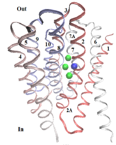
Figure 1: Structure of NCX_Mj viewed from the membrane. The four binding sites shown as four spheres are tightly formed by 8 transmembrane helices labeled by 2 to 5 and 7 to 10. The three green and one blue spheres illustrate three putative Na⁺ binding sites and one Ca²⁺ site, respectively LH16 .

The electric potential $\phi(\mathbf{r})$ from the structure in the biomolecular domain $\Omega_{m}$ is described by the Poisson equation

$$-\epsilon_{m}\epsilon_{0}\nabla^{2}\phi(\mathbf{r})=\sum_{j=1}^{M}q_{j}\delta(\mathbf{r}-\mathbf{r}_{j})\text{, }\forall\mathbf{r}\in\Omega_{m}\text{,}$$ (3)

where $\epsilon_{m}$ is the dielectric constant of biomolecules, $q_{j}$ is the charge of the $j^{\text{th}}$ atom in the NCX protein obtained by the software PDB2PQR DN04 , and $\delta(\mathbf{r}-\mathbf{r}_{j})$ is the Dirac delta function at $\mathbf{r}_{j}$, the coordinate LL12 of that atom. The boundary and interface conditions for $\phi(\mathbf{r})$ in $\Omega$ are

$$\left\{\begin{array}[c]{l}\phi(\mathbf{r})=0\text{ on }\partial\Omega_{D}=\left\{\mathbf{r}\in\partial\Omega\text{: }z=-7\text{ or }z=53\text{ \r{A}}\right\},\\ \nabla\phi(\mathbf{r})\cdot\mathbf{n}=0\text{ on }\partial\Omega_{N}=\left\{\mathbf{r}\in\partial\Omega\text{: }x=\pm 20\text{ or }y=\pm 20\text{ \r{A}}\right\},\\ \left[\phi(\mathbf{r})\right]=\left[\epsilon\epsilon_{0}\nabla\phi(\mathbf{r})\cdot\mathbf{n}\right]=0\text{ on }\partial\Omega_{m}\cap\partial\Omega_{s},\end{array}\right.$$ (4)

where $\mathbf{n}$ is an outward normal unit vector, $\left[u(\mathbf{r})\right]$ is a jump function across the interface $\partial\Omega_{m}\cap\partial\Omega_{s}$ between $\Omega_{s}$ and $\Omega_{m}$, $\epsilon=\epsilon_{s}$ in $\Omega_{s}$, and $\epsilon=\epsilon_{m}$ in $\Omega_{m}$ L13 .

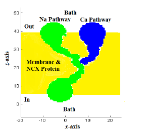
Figure 2: A cross section of 3D simulation domain $\overline{\Omega}=\overline{\Omega}_{s}\cup\overline{\Omega}_{m}$, where the solvent domain $\overline{\Omega}_{s}$ consists of extracellular and intracellular baths (in white) and Na⁺ (green) and Ca²⁺ (blue) pathways, and the biomolecular domain $\overline{\Omega}_{m}$ (yellow) consists of cell membrane and NCX protein LH16 .

III Numerical Methods

To avoid large errors in approximation caused by the delta function $\delta(\mathbf{r}-\mathbf{r}_{j})$ in Eq. (3), the potential function can be decomposed as L13 ; CL03 ; GY07

$$\phi(\mathbf{r})=\left\{\begin{array}[c]{l}\widetilde{\phi}(\mathbf{r})+\phi^{\ast}(\mathbf{r})+\phi^{\text{L}}(\mathbf{r})\text{\ in }\Omega_{m}\\ \widetilde{\phi}(\mathbf{r})\text{ in }\Omega_{s},\end{array}\right.$$ (5)

where $\phi^{\ast}(\mathbf{r})=\sum_{j=1}^{M}q_{j}/(4\pi\epsilon_{m}\left|\mathbf{r-r}_{j}\right|)$ and $\widetilde{\phi}(\mathbf{r})$ is found by solving

$$\left(l_{c}^{2}\Delta-1\right)\nabla\cdot\epsilon_{s}\nabla\widetilde{\phi}(\mathbf{r}) =\rho(\mathbf{r})\text{ in }\Omega_{s}$$ (6)

$$-\nabla\cdot\epsilon_{m}\nabla\widetilde{\phi}(\mathbf{r}) =0\text{ in }\Omega_{m}$$ (7)

without singular source terms $q_{j}\delta(\mathbf{r}-\mathbf{r}_{j})$ and with the interface condition

$$\left[\epsilon\nabla\widetilde{\phi}(\mathbf{r})\cdot\mathbf{n}\right]=\epsilon_{m}\nabla\left(\phi^{\ast}(\mathbf{r})+\phi^{\text{L}}(\mathbf{r}))\right)\cdot\mathbf{n}\text{ on }\partial\Omega_{m}\cap\partial\Omega_{s}\text{.}$$ (8)

The potential function $\phi^{\text{L}}(\mathbf{r})$ is the solution of the Laplace equation

$$\Delta\phi^{\text{L}}(\mathbf{r})=0\text{ in }\Omega_{m}$$ (9)

with the boundary condition

$$\phi^{\text{L}}(\mathbf{r})=\phi^{\ast}(\mathbf{r})\text{ on }\partial\Omega_{m}.$$ (10)

The evaluation of the Green’s function $\phi^{\ast}(\mathbf{r})$ on $\partial\Omega_{m}$ always yields finite numbers and thus avoids the singularity in the solution process.

The Poisson-Fermi (PF) equation (6) is a nonlinear fourth-order PDE in $\Omega_{s}$. Newton’s iterative method is usually used for solving nonlinear problems. We seek the solution $\widetilde{\phi}(\mathbf{r})$ of the linearized PF equation

$$\epsilon_{s}\left(l_{c}^{2}\Delta-1\right)\Delta\widetilde{\phi}-\rho^{\prime}(\widetilde{\phi}_{0})\text{ }\widetilde{\phi}=\rho(\widetilde{\phi}_{0})-\rho^{\prime}(\widetilde{\phi}_{0})\text{ }\widetilde{\phi}_{0}\text{ in }\Omega_{s}\text{,}$$ (11)

where $\widetilde{\phi}_{0}(\mathbf{r})$ is given, $\rho(\widetilde{\phi}_{0})=\sum_{k=1}^{K}q_{k}C_{k}^{0}(\mathbf{r})$, $C_{k}^{0}(\mathbf{r})=C_{k}^{\text{B}}\exp\left(-\beta_{k}\widetilde{\phi}_{0}(\mathbf{r})+\frac{v_{k}}{v_{0}}S_{0}^{\text{trc}}(\mathbf{r})\right)$, $S_{0}^{\text{trc}}(\mathbf{r})=\ln\left(\frac{\Gamma_{0}(\mathbf{r)}}{\Gamma^{\text{B}}}\right)$, $\Gamma_{0}(\mathbf{r)}=1-\sum_{k=1}^{K+1}v_{k}C_{k}^{0}(\mathbf{r})$, $\rho^{\prime}(\widetilde{\phi}_{0})=\sum_{k=1}^{K}\left(-\beta_{k}q_{k}\right)C_{k}^{0}(\mathbf{r})$, and $\rho^{\prime}(\widetilde{\phi})=\frac{d}{d\widetilde{\phi}}\rho(\widetilde{\phi})$. This linear equation is then solved iteratively by replacing the old function $\widetilde{\phi}_{0}$ by newly found solution $\widetilde{\phi}$ and so on until a tolerable approximate potential function $\widetilde{\phi}$ is reached. Note that the differentiation in $\rho^{\prime}(\widetilde{\phi})$ is performed only with respect to $\widetilde{\phi}$ whereas $S^{\text{trc}}$ is treated as another independent variable although $S^{\text{trc}}$ depends on $\widetilde{\phi}$ as well. Therefore, $\rho^{\prime}(\widetilde{\phi}_{0})$ is not exact implying that this is an inexact Newton’s method DE82 that has been shown to be highly efficient in electrostatic calculations for biological systems HS95 ; CH10 .

To avoid numerical complexity in using higher order approximations to the fourth-order derivative, Eq. (11) is reduced to two second-order PDEs L13

PF1 $$:\text{ \ \ }\epsilon_{s}\left(l_{c}^{2}\Delta-1\right)\Psi(\mathbf{r})=\rho(\widetilde{\phi}_{0})\text{ in }\Omega_{s}$$ (12)

PF2 $$:\text{ \ \ }-\epsilon_{s}\Delta\widetilde{\phi}(\mathbf{r})-\rho^{\prime}(\widetilde{\phi}_{0})\text{ }\widetilde{\phi}(\mathbf{r})=-\epsilon_{s}\Psi(\mathbf{r})-\rho^{\prime}(\widetilde{\phi}_{0})\text{ }\widetilde{\phi}_{0}\text{ in }\Omega_{s}$$ (13)

by introducing a density like variable $\Psi=\Delta\widetilde{\phi}$ for which the boundary condition is L13

$$\Psi(\mathbf{r})=0\text{ on }\partial\Omega_{s}.$$ (14)

Eqs. (7), (12), and (13) are coupled together by Eq. (8) in the entire domain $\Omega$. These equations are solved iteratively with an initial guess potential $\widetilde{\phi}_{0}$. Note that the linear PDE (11) (or equivalently (12) and (13)) converges to the nonlinear PDE (6) if $\widetilde{\phi}_{0}$ converges to the exact solution $\widetilde{\phi}$ of Eq. (6).

The standard 7-point finite difference (FD) method is used to discretize all elliptic PDEs (7), (9), (12), and (13), where the interface condition (8) is handled by the simplified matched interface and boundary (SMIB) method proposed in L13 . For simplicity, the SMIB method is illustrated by the following 1D linear Poisson equation (in $x$-axis)

$$-\frac{d}{dx}\left[\epsilon(x)\frac{d}{dx}\widetilde{\phi}(x)\right]=f(x)\text{ in }\Omega$$ (15)

with the interface condition

$$\left[\epsilon\widetilde{\phi}^{\prime}\right]=-\epsilon_{m}\frac{d}{dx}\phi^{\ast}(x)\text{ at }x=\xi=\text{ }\partial\Omega_{m}\cap\partial\Omega_{s}\text{,}$$ (16)

where $\Omega=$ $\Omega_{m}\cup\Omega_{s}$, $\Omega_{m}=(0,$ $\xi)$, $\Omega_{s}=(\xi,$ $L)$, $f(x)=0$ in $\Omega_{m}$, $f(x)\neq 0$ in $\Omega_{s}$, and $\widetilde{\phi}^{\prime}=\frac{d}{dx}\widetilde{\phi}(x)$. The corresponding cases to Eqs. (7), (8), and (13) in $y$- and $z$-axis follow in a similar way. Let two FD grid points $x_{l}$ and $x_{l+1}$ across the interface point $\xi$ be such that $x_{l}<\xi<x_{l+1}$ with $\Delta x=x_{l+1}-x_{l}$, a uniform mesh, for example, as used in this work. The FD equations of the SMIB method at $x_{l}$ and $x_{l+1}$ are

$$\epsilon_{m}\frac{-\widetilde{\phi}_{l-1}+(2-c_{1})\widetilde{\phi}_{l}-c_{2}\widetilde{\phi}_{l+1}}{\Delta x^{2}} =f_{l}+\frac{c_{0}}{\Delta x^{2}}$$ (17)

$$\epsilon_{s}\frac{-d_{1}\widetilde{\phi}_{l}+(2-d_{2})\widetilde{\phi}_{l+1}-\widetilde{\phi}_{l+2}}{\Delta x^{2}} =f_{l+1}+\frac{d_{0}}{\Delta x^{2}},$$ (18)

where

$$c_{1} =\frac{\epsilon_{m}-\epsilon_{s}}{\epsilon_{m}+\epsilon_{s}}\text{, }c_{2}=\frac{2\epsilon_{s}}{\epsilon_{m}+\epsilon_{s}}\text{, }c_{0}=\frac{-\epsilon_{m}\Delta x\left[\epsilon\widetilde{\phi}^{\prime}\right]}{\epsilon_{m}+\epsilon_{s}}\text{, }$$

$$d_{1} =\frac{2\epsilon_{m}}{\epsilon_{m}+\epsilon_{s}}\text{, }d_{2}=\frac{\epsilon_{s}-\epsilon_{m}}{\epsilon_{m}+\epsilon_{s}}\text{, }d_{0}=\frac{-\epsilon_{s}\Delta x\left[\epsilon\widetilde{\phi}^{\prime}\right]}{\epsilon_{m}+\epsilon_{s}}\text{,}$$

$\widetilde{\phi}_{l}$ is an approximation of $\widetilde{\phi}(x_{l})$, and $f_{l}=f(x_{l})$. Note that the jump value $\left[\epsilon\widetilde{\phi}^{\prime}\right]$ at $\xi$ is calculated exactly since the derivative of $\phi^{\ast}$ is given analytically.

After discretization in 3D, the Laplace equation (9), the first PF equation (PF1) (12), or the second PF equation (PF2) (13) coupled with the Poisson equation (7), together with their respective boundary or interface conditions, results in a linear system of algebraic equations $\mathbf{A}\Phi=\mathbf{b}$, where $\mathbf{A}$ is an $N\times N$ symmetric (for Eq. (9) and PF1) or nonsymmetric (for PF2 due to the interface condition) matrix and $\Phi$ and $\mathbf{b}$ are $N\times 1$ unknown and known vectors, respectively. The matrix size $N$ equals to the total number of PD grid points $\left\{\mathbf{r}_{1},\cdots,\mathbf{r}_{N}\right\}$ and depends on the protein size and the uniform mesh size $\Delta x$ in all three axes. For the simulation domain $\Omega$ given in (4), the matrix size is $N=6,246,961$ with $\Delta x=0.5$ Å.

For the NCX protein, the radii of the entrances of the four binding sites in the Na⁺ pathway are about 1.1 Å LH16 . The distances between binding ions and the charged oxygens of chelating amino acid residues are in the range of 2.3 $\sim$ 2.6 Å LH16 . Furthermore, the total number and total charge of these oxygens are 12 and -6.36$e$, respectively LH16 . These indicate that the exchange mechanism of NCX should be investigated at atomic scale. In LH16 , the following atomic model is proposed for studying NCX

$$\phi_{b} =\frac{1}{4\pi\epsilon_{0}}\left(\frac{1}{6}\sum_{k=1}^{6}\left(\sum_{j=1}^{M}\frac{q_{j}}{\epsilon_{p}|c_{j}-A_{k}|}+\sum_{m=1,\text{ }m\neq b}^{8}\frac{O_{m}q_{m}}{\epsilon_{b}|c_{m}-A_{k}|}\right)+\frac{O_{b}q_{b}}{\epsilon_{b}a_{b}}\right),$$ (19)

$$S_{b}^{\text{trc}} =\ln\frac{1-\sum_{m=1}^{8}v_{m}/V_{\text{sites}}}{\Gamma^{\text{B}}},$$ (20)

where $b=$ aS1, bS2, bS3, bS4, aS5, aS6, bS7, or aS8 in Fig. 3, $c_{j}$ is the center of the $j^{\text{th}}$ atom in the NCX protein, $A_{k}$ is one of six symmetric surface points on the spherical site $b$ with radius being either $a_{\text{Na}^{+}}$ or $a_{\text{Ca}^{2+}}$, $|c_{j}-A_{k}|$ is the distance between $c_{j}$ and $A_{k}$, $q_{m}$ denotes the charge of any other site $m=$ aS1,…, aS8 $\neq b$ if $O_{m}\neq 0$ (the site being occupied by an ion, otherwise $O_{m}=0$), $\epsilon_{p}$ is a dielectric constant for the NCX protein, $\epsilon_{b}$ is a dielectric constant in $b$, and $v_{m}$ is the volume of the ion at site $m$ if it is occupied, $v_{m}=0$ otherwise.

The sites bS2, bS3, and bS4 are the three Na⁺ binding (green) sites in Fig. 1 and bS7 is the Ca²⁺ binding (blue) site. The sites aS1 and aS5 are two access sites in the Na⁺ pathway to the binding sites whereas aS6 and aS8 are access sites in the Ca²⁺ pathway as shown in Fig. 3. The coordinates of the binding sites (bS2, bS3, bS4, bS7) and the access sites (aS1, aS5, aS6, aS8) are determined by the crystallized structure in LL12 and the empirical method in LH16 , respectively. These eight sites are numbered by assuming exchanging paths in which Na⁺ ions move inwards from extracellular to intracellular bath and Ca²⁺ ions move outwards from intracellular to extracellular bath without changing direction. The bidirectional ion exchange suggests a conformational change between the outward- (Fig. 3A) and inward-facing (Fig. 3B) states of NCX LL12 . The outward-facing structure is shown in Figs. 1 and 2. The inward-facing structure has not yet been seen in X-ray, but Liao et al. LL12 have proposed an intramolecular homology model by swapping TMs 6-7A and TMs 1-2A (in Fig. 1) helices to create an inwardly facing structure of NCX_Mj. Numerically, we simply reverse the z-coordinate of all protein atoms in Fig. 2 with respective to the center point of the NCX structure LH16 .

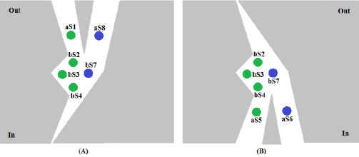
Figure 3: In (A) outward-facing structure and (B) inward-facing homology conformations, the eight sites aS1, bS2,$...$, aS8 marked in green and blue disks located in the Na⁺ (green) and Ca²⁺ (blue) pathways, respectively, are used for electrostatic analysis, where bS2, bS3, bS4, and bS7 are binding sites shown in Fig. 1 and aS1, aS5, aS6, and aS8 are access sites to the binding sites (binding pocket).

It is shown in LH16 that numerical results produced by the Poisson-Fermi model agreed with experimental results on the 3Na${}^{+}:2$Ca²⁺ stoichiometry of NCX, i.e., NCX extrudes 2 intracellular Ca²⁺ ions across the cell membrane against [Ca²⁺] gradient in exchange with 3 extracellular Na⁺ ions using only the energy source of [Na⁺] downhill gradient. The stoichiometric mechanism described by PF is based on a transport cycle of state energy changes by the electric and steric forces on Na⁺ and Ca²⁺ ions occupying or unoccupying their respective access or binding sites in the NCX structure. The energy state of each occupied or unoccupied site was obtained by the electric and steric formulas (19) and (20). Five energy (total potential) states (TPS) have been proposed and calculated to establish the cyclic exchange mechanism in LH16 . The 5 TP states (with their occupied sites) are TPS1 (bS3, bS7), TPS2 (aS1, bS3, bS7), TPS3 (aS1, bS2, bS4, bS7), TPS4 (bS2, bS3, bS4), and TPS5 (bS2, bS3, bS4), where TPS1 and TPS5 are in the inward-facing configuration and TPS2, TPS3 and TPS4 in the outward-facing configuration as shown in Fig. 4. The transport cycle is a sequence of changing states in the following order: TPS1 $\rightarrow$ TPS2 $\rightarrow$ TPS3 $\rightarrow$ TPS4 $\rightarrow$ TPS5 $\rightarrow$ TPS1 as shown in Fig. 4. TPS1 is changed to TPS2 and TPS3 when the extracellular bath concentration $\left[\text{Na}^{+}\right]_{\text{o}}$ of sodium ions is sufficiently large for one more Na⁺ to occupy aS1 (in TPS2) or even two more Na⁺ to occupy aS1 and bS2 (TPS3) such that these two Na⁺ ions have sufficient (positive) energy to extrude the Ca²⁺ at bS7 in TPS3 out of the binding pocket to become TPS4. It is postulated in LH16 that the conformational change of NCX is induced by the absence or presence of Ca²⁺ at the binding site bS7 as shown in Fig. 4. After NCX is changed from the outward-facing configuration in TPS4 to the inward-facing configuration in TPS5, a Ca²⁺ can access aS6 and then move to bS7 in TPS1 if the intracellular bath concentration $\left[\text{Ca}^{2+}\right]_{\text{i}}$ of calcium ions is sufficiently large. Using Eqs. (1), (19), and (20), the selectivity ratio of Na⁺ to Ca²⁺ by NCX from the extracellular bath to the binding site bS2 in TPS1 (after the conformational change) is defined and given as LH16

$$\frac{C_{\text{Na}^{+}}(\mathbf{r})}{C_{\text{Ca}^{2+}}(\mathbf{r})}=\frac{\left[\text{Na}^{+}\right]_{\text{o}}\exp\left(-q_{\text{Na}^{+}}\Psi_{\text{bS2}}^{\text{TPS1}}\right)}{\left[\text{Ca}^{2+}\right]_{\text{o}}\exp\left(-q_{\text{Ca}^{2+}}\Psi_{\text{bS2}}^{\text{TPS1}}\right)}=55.4$$ (21)

under the experimental bath conditions $\left[\text{Na}^{+}\right]_{\text{o}}$ and $\left[\text{Ca}^{2+}\right]_{\text{o}}$ given in Table 1, where $\Psi_{b}=(q_{b}\phi_{b}-S_{b}^{\text{trc}}k_{B}T)/q_{b}$. The selectivity ratio of Ca²⁺ to Na⁺ by NCX from the intracellular bath to the binding site bS7 in TPS4 is

$$\frac{C_{\text{Ca}^{2+}}(\mathbf{r})}{C_{\text{Na}^{+}}(\mathbf{r})}=\frac{\left[\text{Ca}^{2+}\right]_{\text{i}}\exp\left(-q_{\text{Ca}^{2+}}\Psi_{\text{bS7}}^{\text{TPS4}}\right)}{\left[\text{Na}^{+}\right]_{\text{i}}\exp\left(-q_{\text{Na}^{+}}\Psi_{\text{bS7}}^{\text{TPS4}}\right)}=4986.1.$$ (22)

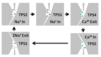
Figure 4: A transport cycle of changing total potential (TP) states of Na ions (green) and Ca ions (blue) entering and exiting the binding pocket in the order TPS1 $\rightarrow$ TPS2 $\rightarrow$ TPS3 $\rightarrow$ TPS4 $\rightarrow$ TPS5 $\rightarrow$ TPS1 is proposed in LH16 to establish the NCX stoichiometric mechanism.

Table 1: Values of Model Notations Symbol Meaning  Value  Unit $k_{B}$ Boltzmann constant $1.38\times 10^{-23}$ J/K $T$ temperature $298.15$ K $e$ proton charge $1.602\times 10^{-19}$ C $\epsilon_{0}$ permittivity of vacuum $8.85\times 10^{-14}$ F/cm $\epsilon_{b}$, $\epsilon_{p}$, $\epsilon_{s}$, $\epsilon_{m}$ dielectric constants $10$, $20$, $78.45$, 2 $l_{c}=2a_{i}$ correlation length $i=\text{Na}^{+}\text{, Ca}^{2+}$ Å $a_{\text{Na}^{+}}$, $a_{\text{Ca}^{2+}}$ radii $0.95$, $0.99$ Å $a_{\text{Cl}^{-}}$, $a_{\text{H}_{2}\text{O}}$ radii $1.81$, $1.4$ Å $O_{m}^{b}$ site occupancy 0 or 1 $\left[\text{Na}^{+}\right]_{\text{o}}$, $\left[\text{Na}^{+}\right]_{\text{i}}$ bath concentrations 120, 60 LL12 mM $\left[\text{Ca}^{2+}\right]_{\text{o}}$, $\left[\text{Ca}^{2+}\right]_{\text{i}}$ bath concentrations 1, 33 LL12 $\mu$M i, o intra, extracellular

We need to extend the energy profile of each TPS in the filter region $\Omega_{f}$ $\subset\Omega_{s}$, which contains the access and binding sites shown in Fig. 3, to the entire simulation domain $\Omega$ with boundary conditions in which the membrane potential and bath concentrations [Ca²⁺] and [Na⁺] are given, since the exchange cycle inside the binding pocket is driven by these far field boundary conditions. Therefore, the total energy of an ion in the filter region in a particular state is determined by all ions and water molecules in the system with boundary potentials and is calculated by the continuum model (12) and (13) in $\overline{\Omega}_{s}\backslash\Omega_{f}$ and the atomic model (19) and (20) in $\Omega_{f}$. The values of $\phi_{b}$ and $S_{b}^{\text{trc}}$ of the atomic model can be used as Dirichlet boundary values for the continuum model. Since all ions and water are treated as hard spheres with interstitial voids, the algebraic steric potential $S_{b}^{\text{trc}}$ is consistent with the continuous steric function $S^{\text{trc}}(\mathbf{r})$. The algebraic electric potential $\phi_{b}$ is based on Coulomb’s law in stead of Poisson’s theory. Therefore, the PF theory is a continuum-molecular theory. We refer to LH16 for more details.

IV GPU Algorithms

We first describe a nonlinear solver of inexact-Newton type in Table 2 for the PF model (1) and (2) for sequential coding, where $\left\|\Phi\right\|_{\infty}$ is the maximum norm of the $N\times 1$ vector $\Phi$, $\omega_{\text{PF}}=0.3$ is a relaxation parameter, and ErrTol $=10^{-3}$ is an error tolerance for Newton’s iteration. The error tolerance of linear solvers is $10^{-6}$ for all algebraic systems ($\mathbf{A}^{\text{L}}\Phi^{\text{L}}=\mathbf{b}^{\text{L}}$, $\mathbf{A}_{0}\Phi_{0}=\mathbf{b}_{0}$, $\mathbf{A}^{\text{PF1}}\Psi=\mathbf{b}^{\text{PF1}}$, $\mathbf{A}^{\text{PF2}}\Phi=\mathbf{b}^{\text{PF2}}$) in Steps 1 - 4. The vectors $\Phi^{\text{L}}$, $\Phi_{0}$, $\Psi$, and $\Phi$ are approximate solutions of $\phi^{\text{L}}(\mathbf{r})$, $\widetilde{\phi}_{0}(\mathbf{r})$, $\Psi(\mathbf{r})$, and $\widetilde{\phi}(\mathbf{r})$, respectively, at FD grid points $\mathbf{r}\in\left\{\mathbf{r}_{1},\cdots,\mathbf{r}_{N}\right\}$. The $N\times N$ matrix $\mathbf{A}$ with entries $a_{ij}$ of each linear system in Table 2 is compressed to seven $N\times 1$ vectors A0[i], $\cdots$, A6[i] for i = 0, …, $N$-1, where $a_{ij}$ = A0[i] with $j=$ i, A1[i] with $j=$ i+1 (the east neighboring point of i), A2[i] with $j=$ i-1 (west), A3[i] with $j=$ i-XPts (south), A4[i] with $j=$ i+XPts (north), A5[i] with $j=$ i-XPts*YPts (downside), or A6[i] with $j=$ i+XPts*YPts (upside), and XPts and YPts are total numbers of grid points in the $x$- and $y$-axis, respectively. Therefore, the matrix is stored in a diagonal format without offset arrays BG08 . It has been shown in BG08 that the diagonal representation of sparse matrices is memory-bandwidth efficient and has high computational intensity for the matrix-vector multiplication on CUDA.

Table 2: Sequential Algorithm of PF Nonlinear Solver
1	Solve Eqs. (9), (10) in $\overline{\Omega}_{m}$ for $\phi^{\text{L}}(\mathbf{r})$ in the discrete form $\mathbf{A}^{\text{L}}\Phi^{\text{L}}=\mathbf{b}^{\text{L}}$
	by a linear solver (LS).
2	Solve PF2 Eqs. (4), (7), (8), (13) with $\rho^{\prime}=\Psi=0$ in $\overline{\Omega}\backslash\Omega_{f}$ for $\widetilde{\phi}_{0}(\mathbf{r})$
	in $\mathbf{A}_{0}\Phi_{0}=\mathbf{b}_{0}$ by LS.
3	Solve PF1 Eq. (12), (14)$\text{ in }\overline{\Omega}_{s}\backslash\Omega_{f}$ for $\Psi(\mathbf{r})$ in $\mathbf{A}^{\text{PF1}}\Psi=\mathbf{b}^{\text{PF1}}$ by LS.
4	Solve PF2 Eqs. (4), (7), (8), (13)$\text{ in }\overline{\Omega}_{s}\backslash\Omega_{f}$ for $\widetilde{\phi}(\mathbf{r})$ in $\mathbf{A}^{\text{PF2}}\Phi=\mathbf{b}^{\text{PF2}}$ by LS.
5	Assign $\Phi:=\omega_{\text{PF}}\Phi_{0}+(1-\omega_{\text{PF}})\Phi$.
	If $\left\|\Phi-\Phi_{0}\right\|_{\infty}$ $>$ ErrTol, $\Phi_{0}:=\Phi$ (i.e., $\widetilde{\phi}_{0}:=\widetilde{\phi}$) and go to Step 3; else stop.

The conjugate gradient (CG) method is one of the most efficient and widely used linear solvers for the Poisson-Boltzmann equation in biomolecular applications HS95 ; DM89 ; NH91 ; WL10 . Since the PF2 linear system is nonsymmetric, we use the Bi-CGSTAB method of Van der Vorst V92 , which is probably the most popular short recurrence method for large-scale nonsymmetric linear systems SS10 .

The parallel platform CUDA created by NVIDIA is an application programming interface software that gives direct access to the GPU’s virtual instruction set and parallel computational elements and works with programming languages C, C++, and Fortran A08 ; NB08 . Our sequential code is written in C++. GPU programming is substantially simplified by using CUDA. For example, we only need to replace CPU_BiCGSTAB() by GPU_BiCGSTAB() in the same line of the function call without changing any other parts of the code, i.e., CUDA generates a sequential code if CPU_BiCGSTAB() is called or a parallel code if GPU_BiCGSTAB() is called. Of course, the function definition of GPU_BiCGSTAB() is different from that of CPU_BiCGSTAB(). We now describe our GPU implementation of the Bi-CGSTAB method BB94 (with pointwise Jacobi preconditioning) as shown by the algorithm in Table 3, where the symbol C: or G: indicates that the corresponding statement is executed at the host (CPU) or the device (GPU).

Table 3: GPU Algorithm 1 for Bi-Conjugate Gradient Stabilized Method
1 C: Copy $\mathbf{A}$, $\mathbf{b}$ and initial guess $\mathbf{x}^{(0)}$ from host (C) to device (G).
2 G: Compute $\mathbf{r}^{(0)}=\mathbf{b}-\mathbf{Ax}^{(0)}$ and set $\mathbf{\tilde{r}}=\mathbf{r}^{(0)}.$
3 C: for $i=1,2,...$
4 G:      $\rho_{i-1}=\mathbf{\tilde{r}}^{T}\mathbf{r}^{(i-1)}$ with CUDA Reduction Method (RM) H07
5 C:      if $i=1$
6 G:      $\ \ \ \mathbf{p}^{(i)}=\mathbf{r}^{(i-1)}$
7 C:      else
8 G:     $\ \ \ \ \ \beta_{i-1}=(\rho_{i-1}\alpha_{i-1})/(\rho_{i-2}\omega_{i-1})$
9 G:     $\ \ \ \ \ \mathbf{p}^{(i)}=\mathbf{r}^{(i-1)}+\beta_{i-1}(\mathbf{p}^{(i-1)}-\omega_{i-1}\mathbf{v}^{(i-1)})$
10 C:     end
11 G: $\ \ \ \ \mathbf{v}^{(i)}=\mathbf{Ap}^{(i)}$
12 G:      $\alpha_{i}=\rho_{i-1}/\mathbf{\tilde{r}}^{T}\mathbf{v}^{(i)}$ with RM
13 G:      $\mathbf{s}=\mathbf{r}^{(i-1)}-\alpha_{i}\mathbf{v}^{(i)}$
14 G:      $\mathbf{t}=\mathbf{As}$
15 G:      $\omega_{i}=\mathbf{t}^{T}\mathbf{s}/\mathbf{t}^{T}\mathbf{t}$ with RM
16 G:      $\mathbf{x}^{(i)}=\mathbf{x}^{(i-1)}+\alpha_{i}\mathbf{p}^{(i)}+\omega_{i}\mathbf{s}$
17 G:      $\mathbf{r}^{(i)}=\mathbf{s}-\omega_{i}\mathbf{t}$
18 G:      Evaluate $\left\|\mathbf{r}^{(i)}\right\|_{\infty}$ with RM and then copy $\left\|\mathbf{r}^{(i)}\right\|_{\infty}$ to host.
19 C:       If $\left\|\mathbf{r}^{(i)}\right\|_{\infty}<$ ErrTol,
20 G:         copy $\mathbf{x}^{(i)}$ to host and stop.
21 C: end

The computational complexity of GPU Algorithm 1 is dominated by (A) the execution time of (i) the matrix-vector products in Steps 2, 11, and 14 and (ii) the vector inner products in Steps 4, 12, and 15; and (B) the synchronization time of threads within a block to share data through shared memory NB08 . The CPU and GPU systems used for this work are Intel Xeon E5-1650 and NVIDIA GeForce GTX TITAN X (with 3072 CUDA cores), respectively. The total numbers of blocks and threads per block defined in our GPU code were 256 and 1024, respectively, with which the inner product of two vectors of dimension $N=$ 6,246,961, for example, is processed with $256\times 1024=$ 262,144 threads of execution. A while loop with a stride of 262,144 is hence incorporated into the kernel in order to visit all vector elements. Each thread can access to its private local memory, its shared memory, and the same global memory of all threads NB08 . The fine-grained data parallelism of these vectors is expressed by $256$ blocks in shared memory. The thread parallelism on GPU multiprocessors (cores) is transparently scaled and scheduled by CUDA NB08 . In order to keep all multiprocessors on the GPU busy, the inner product of these very large vectors (arrays) is performed using a parallel reduction method proposed in H07 . Parallel reduction is a fundamental technique to process very large arrays in parallel blocks by recursively reducing a portion of the array within each thread block. The inner-product operation reduces two vectors to a single scalar.

The matrix $\mathbf{A}^{\text{PF2}}$ and the vectors $\mathbf{b}^{\text{PF1}}$ and $\mathbf{b}^{\text{PF2}}$ in Table 2 (the sequential nonlinear solver) need to be updated iteratively according to Eqs. (12) and (13). Iterative switches between the sequential code on CPU for updating these matrix and vectors (Step 1 in Table 3) and the parallel code on GPU for solving linear systems (other Steps in Table 3) drastically reduce the parallel performance of GPU. It is thus crucial to parallelize the nonlinear solver for which we propose an algorithm in Table 4, where the matrices $\mathbf{A}^{\text{L}}$ (in Step 2), $\mathbf{A}_{0}$ (Step 4), $\mathbf{A}^{\text{PF1}}$ (Step 5), and $\mathbf{A}^{\text{PF2}}$ (Step 6) are all stored in A0[i], $\cdots$, A6[i] and constructed on GPU. The corresponding vectors $\mathbf{b}^{\text{L}}$, $\mathbf{b}_{0}$, $\mathbf{b}^{\text{PF1}}$, and $\mathbf{b}^{\text{PF2}}$ are similarly stored in $\mathbf{b}$ and constructed on GPU. Step 1 in Table 3 is now removed. Note that $\mathbf{A}^{\text{PF2}}$, $\mathbf{b}^{\text{PF1}}$ and $\mathbf{b}^{\text{PF2}}$ are updated iteratively on GPU since $\Phi$ (corresponding to $\widetilde{\phi}(\mathbf{r})$) is updated iteratively. The vector $\mathbf{b}^{\text{IF}}$ corresponding to the right-hand side of the interface equation (8) is calculated once in Step 3 on CPU and repeatedly used in Steps 4 and 6 on GPU.

Table 4: GPU Algorithm 2 for Poisson-Fermi Nonlinear Solver
1 C:	Allocate the vectors A0[i], $\cdots$, A6[i], $\mathbf{b}$, $\Phi^{\text{L}}$, $\Psi$, $\Phi_{0}$, $\Phi$ and $\mathbf{b}^{\text{IF}}$ on the global
	memory of the GPU.
2 G:	Solve Eqs. (9), (10) in $\overline{\Omega}_{m}$ for $\phi^{\text{L}}(\mathbf{r})$ once in $\mathbf{A}^{\text{L}}\Phi^{\text{L}}=\mathbf{b}^{\text{L}}$ by GPU Algorithm 1.
3 C:	Compute the interface vector $\mathbf{b}^{\text{IF}}$ and copy it from host to device.
4 G:	Solve PF2 Eqs. (4), (7), (8), (13) with $\rho^{\prime}=\Psi=0$ in $\overline{\Omega}\backslash\Omega_{f}$ for $\widetilde{\phi}_{0}(\mathbf{r})$
	in $\mathbf{A}_{0}\Phi_{0}=\mathbf{b}_{0}$ by GPU Algorithm 1.
5 G:	Solve PF1 Eqs. (12), (14)$\text{ in }\overline{\Omega}_{s}\backslash\Omega_{f}$ for $\Psi(\mathbf{r})$ in $\mathbf{A}^{\text{PF1}}\Psi=\mathbf{b}^{\text{PF1}}$
	by GPU Algorithm 1.
6 G:	Solve PF2 Eqs. (4), (7), (8), (13) in $\overline{\Omega}\backslash\Omega_{f}$ for $\widetilde{\phi}(\mathbf{r})$ in $\mathbf{A}^{\text{PF2}}\Phi=\mathbf{b}^{\text{PF2}}$
	by GPU Algorithm 1.
7 G:	Assign $\Phi:=\omega_{\text{PF}}\Phi_{0}+(1-\omega_{\text{PF}})\Phi$. If $\left\|\Phi-\Phi_{0}\right\|_{\infty}$ $>$ ErrTol, $\Phi_{0}:=\Phi$ and
	go to Step 5; else stop.

V Results

We first present some physical results obtained by the PF model. For TPS3 in Fig. 4, the electric potential profiles of $\phi(\mathbf{r})$ along the axes of Na⁺ and Ca²⁺ pathways (Fig. 2) are shown in Fig. 5 in green and blue curves, respectively. Each curve was obtained by averaging the values of $\phi(\mathbf{r})$ at cross sections along the axis of the solvent domain $\Omega_{s}$ that contains both two baths and a pathway. The potential values at aS1, bS2, bS3, bS4, bS7, and aS8 were obtained by Eq. (19) whereas the value at aS9 was obtained by Eqs. (12) and (13). These two curves suggest opposite flows of Na⁺ and Ca²⁺ ions as illustrated in the figure. Numerical results presented here are only for TPS3 as those of the other four states in Fig. 4 follow in the same way of calculation with four times more computational efforts.

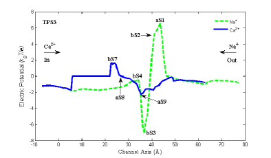
Figure 5: For TPS3 in Fig. 4, the electric potential profiles of $\phi(\mathbf{r})$ along the axes of Na⁺ and Ca²⁺ pathways are shown in green and blue curves, respectively. Each curve was obtained by averaging the values of $\phi(\mathbf{r})$ at cross sections along the axis of the solvent domain $\Omega_{s}$ that contains both two baths and a pathway. The notations aS1, bS2, bS3, bS4, bS7, aS8, and aS9 indicate the potential values at those sites. The potential profiles suggest opposite flows of Na⁺ and Ca²⁺ ions as illustrated in the figure.

We next show the speedup of the parallel (GPU) computation over the sequential (CPU) computation in Table 5, where the time is in second, the linear solver is described in Table 3 for the parallel version that yields the sequential version by replacing the symbol G: by C:, and the nonlinear solver is described in Tables 2 and 4 for the CPU and GPU version, respectively. The speedup in total runtime is drastically reduced from 16.9 to 1890/370 = 5.1 if the nonlinear solver is not parallelized although the speedup of linear solver alone is 22.8, where 370 (not shown in the table) is the total runtime of the mixed algorithm of sequential nonlinear and parallel linear solvers. It is thus important to parallelize the nonlinear solver of the coupled nonlinear PDEs, such as the Poisson-Fermi model, in scientific computing since most realistic applications in engineering or scientific systems are highly nonlinear. The reduction of speedups from 22.8 (in linear solver time) to 16.9 (in total runtime) is due mainly to the lower efficiency of GPU compared to that of CPU for constructing matrix systems in Steps 4, 5, and 6 in GPU Algorithm 2 as shown by the smaller speedup 7.7 (in nonlinear solver time) in Table 5. Nevertheless, the GPU algorithms of the linear and nonlinear solver in Tables 3 and 4 for the Poisson-Fermi model improve significantly the speedups of 7-10 in previous GPU studies for Poisson, linear Poisson-Boltzmann, and nonlinear Poisson-Boltzmann solvers SK13 ; CO13 .

Table 5: Speedup of GPU over CPU
	CPU (T1)	GPU (T2)	Speedup (T1/T2)
Linear Solver Time in Sec.	$1551$	$68$	$22.8$
Nonlinear Solver Time	$339$	$44$	$7.7$
Total Runtime	$1890$	$112$	$16.9$

VI Conclusion

We propose two GPU (parallel) algorithms for biological ion channel simulations using the Poisson-Fermi model that extends the classical Poisson-Boltzmann model to study not only the continuum but also the atomic properties of ions and water molecules in highly charged ion channel proteins. These algorithms exploit the thread and data parallelism on GPU with the CUDA platform that makes GPU programming easier and GPU computing more efficient. Numerical methods for both linear and nonlinear solvers in the algorithms are given in detail to illustrate the salient features of CUDA in implementation. These parallel algorithms on GPU are shown to achieve 16.9$\times$ speedup over the sequential algorithms on CPU, which is better than that of previous GPU algorithms based on the Poisson-Boltzmann model.

- (1) K. A. Sharp and B. Honig, Electrostatic interactions in macromolecules: Theory and applications, Annu. Rev. Biophys. Biophys. Chem. 19, 301-332 (1990).
- (2) W. Humphrey, A. Dalke, and K. Schulten, VMD - Visual Molecular Dynamics, J. Molec. Graphics, 14, 33-38 (1996).
- (3) N. A. Baker, et al., Electrostatics of nanosystems: application to microtubules and the ribosome, Proc. Natl. Acad. Sci. 98,10037-10041 (2001).
- (4) T. J. Dolinsky, et al., PDB2PQR: an automated pipeline for the setup of Poisson–Boltzmann electrostatics calculations, Nucleic Acids Res. 32, W665-W667 (2004).
- (5) D. A. Case, et al., The Amber biomolecular simulation programs, J. Comput. Chem. 26, 1668-1688 (2005).
- (6) B. R. Brooks, et al., CHARMM: the biomolecular simulation program, J. Comput. Chem. 30, 1545-1614 (2009).
- (7) J. D. Owens, et al., GPU computing, Proceedings of the IEEE 96.5, 879-899 (2008).
- (8) J. Nickolls and W. J. Dally, The GPU computing era, IEEE micro 30.2 (2010).
- (9) J.-L. Liu, Numerical methods for the Poisson-Fermi equation in electrolytes, J. Comput. Phys. 247, 88-99 (2013).
- (10) J.-L. Liu and B. Eisenberg, Correlated ions in a calcium channel model: a Poisson-Fermi theory, J. Phys. Chem. B 117, 12051-12058 (2013).
- (11) J.-L. Liu and B. Eisenberg, Poisson-Nernst-Planck-Fermi theory for modeling biological ion channels, J. Chem. Phys. 141, 22D532 (2014).
- (12) J.-L. Liu and B. Eisenberg, Analytical models of calcium binding in a calcium channel, J. Chem. Phys. 141, 075102 (2014).
- (13) J.-L. Liu and B. Eisenberg, Numerical methods for a Poisson-Nernst-Planck-Fermi model of biological ion channels, Phys. Rev. E 92, 012711 (2015).
- (14) J.-L. Liu and B. Eisenberg, Poisson-Fermi model of single ion activities in aqueous solutions, Chem. Phys. Lett. 637, 1-6 (2015).
- (15) J.-L. Liu, H.-j. Hsieh, and B. Eisenberg, Poisson-Fermi modeling of the ion exchange mechanism of the sodium/calcium exchanger, J. Phys. Chem. B 120, 2658-2669 (2016).
- (16) D. Xie, J.-L. Liu, and B. Eisenberg, Nonlocal Poisson-Fermi model for ionic solvent, Phys. Rev. E 94, 012114 (2016).
- (17) J.-L. Liu, D. Xie, and B. Eisenberg, Poisson-Fermi formulation of nonlocal electrostatics in electrolyte solutions, to appear in Mol. Based Math. Biol. (2017).
- (18) A. Warshel and S. T. Russell, Calculations of electrostatic interactions in biological systems and in solutions, Q. Rev. Biophys. 17, 283-422 (1984).
- (19) M. E. Davis and J. A. McCammon, Electrostatics in biomolecular structure and dynamics, Chem. Rev. 90, 509-521 (1990).
- (20) B. Honig and A. Nicholls, Classical electrostatics in biology and chemistry, Science 268, 1144-1149 (1995).
- (21) D. Andelman, Electrostatic properties of membranes: The Poisson-Boltzmann theory, in R. Lipowsky and E. Sackmann, Eds., Handbook of Biological Physics, Elsevier, 1, 603-642 (1995).
- (22) P. Attard, Electrolytes and the electric double layer, Adv. Chem. Phys. 92, 1-159 (1996).
- (23) V. Vlachy, Ionic effects beyond Poisson-Boltzmann theory, Annu. Rev. Phys. Chem. 50, 145-165 (1999).
- (24) R. R. Netz and H. Orland, Beyond Poisson-Boltzmann: fluctuation effects and correlation functions, Eur. Phys. J. E 1, 203-214 (2000).
- (25) A. A. Kornyshev, Double-layer in ionic liquids: Paradigm change? J. Phys. Chem. B 111, 5545-5557 (2007).
- (26) P. Grochowski and J. Trylska, Continuum molecular electrostatics, salt effects and counterion binding–A review of the Poisson-Boltzmann model and its modifications, Biopolymers 89, 93-113 (2008).
- (27) M. Z. Bazant, M. S. Kilic, B. D. Storey, and A. Ajdari, Towards an understanding of induced-charge electrokinetics at large applied voltages in concentrated solutions, Adv. Coll. Interf. Sci. 152, 48-88 (2009).
- (28) B. Eisenberg, Crowded charges in ion channels, in Advances in Chemical Physics, S. A. Rice, Ed., John Wiley & Sons, Inc. 148, 77-223 (2011).
- (29) M. Gouy, Sur la constitution de la charge electrique a la surface d’un electrolyte (Constitution of the electric charge at the surface of an electrolyte), J. Phys. 9, 457-468 (1910).
- (30) D. L. Chapman, A contribution to the theory of electrocapillarity, Phil. Mag. 25, 475-481 (1913).
- (31) H. A. Van der Vorst, Bi-CGSTAB: A fast and smoothly converging variant of Bi-CG for the solution of nonsymmetric linear systems, SIAM J. Sci. and Stat. Comput. 13, (1992) 631-644.
- (32) R. Barrett, M. Berry, T. F. Chan, J. Demmel, J. Donato, J. Dongarra , V. Eijkhout, R. Pozo, C. Romine, and H. Van der Vorst, Templates for the Solution of Linear Systems: Building Blocks for Iterative Methods, (2nd Ed., SIAM, Philadelphia, 1994).
- (33) J. Liao, H. Li, W. Zeng, D. B. Sauer, R. Belmares, and Y. Jiang, Structural insight into the ion-exchange mechanism of the sodium/calcium exchanger, Science 335, 686-690 (2012).
- (34) N. A. Simakov and M. G. Kurnikova, Graphical processing unit accelerated poisson equation solver and its application for calculation of single ion potential in ion-channels, Molecular Based Mathematical Biology 1, 151-163 (2013).
- (35) J. Colmenares, J. Ortiz, and W. Rocchia, GPU linear and non-linear Poisson-Boltzmann solver module for DelPhi, Bioinformatics, btt699 (2013).
- (36) C. D. Santangelo, Computing counterion densities at intermediate coupling, Phys. Rev. E 73, 041512 (2006).
- (37) Berman, H. M., Westbrook, J., Feng, Z., Gilliland, G., Bhat, T. N., Weissig, H., … & Bourne, P. E., The protein data bank. Nucleic acids research, 28(1), 235-242 (2000). H. M. Berman et al., Acta Cryst. D58, 899 (2002).
- (38) T. J. Dolinsky, P. Czodrowski, H. Li, J. E. Nielsen, J. H. Jensen, G. Klebe, and N. A. Baker, PDB2PQR: expanding and upgrading automated preparation of biomolecular structures for molecular simulations, Nucleic Acids Res. 35, W522-W525 (2007).
- (39) I-L. Chern, J.-G. Liu, and W.-C. Wang, Accurate evaluation of electrostatics for macromolecules in solution, Methods Appl. Anal. 10, 309-328 (2003).
- (40) W. Geng, S. Yu, and G. Wei, Treatment of charge singularities in implicit solvent models, J. Chem. Phys. 127, 114106 (2007).
- (41) R. S. Dembo, S. C. Eisenstat, and T. Steihaug, Inexact Newton methods, SIAM J. Numer. Anal. 19, 400-408 (1982).
- (42) M. Holst and F. Saied, Numerical solution of the nonlinear Poisson-Boltzmann equation: Developing more robust and efficient methods, J. Comput. Chem. 16, 337-364 (1995).
- (43) Q. Cai, M. J. Hsieh, J. Wang, R. Luo, Performance of nonlinear finite-difference Poisson- Boltzmann solvers, J. Chem. Theory Comput. 6, 203-211 (2010).
- (44) M. E. Davis and J. A. McCammon, Solving the finite difference linearized Poisson-Boltzmann equation: A comparison of relaxation and conjugate gradient methods, J. Comput. Chem. 10, 386-391 (1989).
- (45) A. Nicholls and B. Honig, A rapid finite difference algorithm, utilizing successive over-relaxation to solve the Poisson-Boltzmann equation, J. Comput. Chem. 12, 435-445 (1991).
- (46) J. Wang and R. Luo, Assessment of linear finite-difference Poisson-Boltzmann solvers, J. Comput. Chem. 31, 1689-1698 (2010).
- (47) G. L. G. Sleijpen, P. Sonneveld, and M. B. Van Gijzen, Bi-CGSTAB as an induced dimension reduction method, Appl. Numer. Math. 60, 1100-1114 (2010).
- (48) F. Abi-Chahla, Nvidia’s CUDA: The End of the CPU?, Tom’s Hardware, June 18, 2008.
- (49) N. Bell and M. Garland, Efficient sparse matrix-vector multiplication on CUDA, Vol. 2. No. 5. Nvidia Technical Report, Nvidia Corporation, 2008.
- (50) J. Nickolls, I. Buck, M. Garland, and K. Skadron, Scalable parallel programming with CUDA, Queue 6, (2008) 40-53.
- (51) M. Harris, Optimizing parallel reduction in CUDA, Nvidia Developer Technology, Nvidia Corporation, 2007.