Kernelized Hashcode Representations for Relation Extraction

Abstract

Kernel methods have produced state-of-the-art results for a number of NLP tasks such as relation extraction, but suffer from poor scalability due to the high cost of computing kernel similarities between natural language structures. A recently proposed technique, kernelized locality-sensitive hashing (KLSH), can significantly reduce the computational cost, but is only applicable to classifiers operating on kNN graphs. Here we propose to use random subspaces of KLSH codes for efficiently constructing an explicit representation of NLP structures suitable for general classification methods. Further, we propose an approach for optimizing the KLSH model for classification problems by maximizing an approximation of mutual information between the KLSH codes (feature vectors) and the class labels. We evaluate the proposed approach on biomedical relation extraction datasets, and observe significant and robust improvements in accuracy w.r.t. state-of-the-art classifiers, along with drastic (orders-of-magnitude) speedup compared to conventional kernel methods.

1 Introduction

As the field of biomedical research expands very rapidly, developing tools for automated information extraction from biomedical literature becomes a necessity. In particular, the task of identifying biological entities and their relations from scientific papers has attracted significant attention in the past several years (?; ?; ?), especially because of its potential impact on developing personalized cancer treatments (?; ?; ?). See Fig. 1 for an example of the relation extraction task.

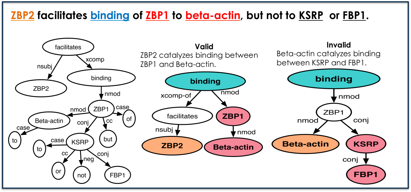
Figure 1: On the left, a parse tree of a sentence is shown. In the sentence, the tokens corresponding to bio-entities (proteins, chemicals, etc.) or interaction types are underlined. We highlight the result of extracting one relation from the sentence, using color-coding for its constituents: an interaction type (green) and bio-entities either participating in the interaction (red), or catalyzing it (orange). From two extraction candidates (valid/invalid), we obtain subgraphs from the parse tree, used as structural features for binary classification of the candidates.

For the relation extraction task, approaches based on convolution kernels (?) have demonstrated state-of-the-art performance  (?; ?). However, despite their success and intuitive appeal, the traditional kernel-trick based methods can suffer from relatively high computational costs, since computing kernel similarities between two natural language structures (graphs, paths, sequences, etc.) can be an expensive operation. Furthermore, to build a support vector machine (SVM) or a k-nearest neighbor (kNN) classifier from $N$ training examples, one needs to compute kernel similarities between $O(N^{2})$ pairs of training points, which can be prohibitively expensive for large $N$. Some approximation methods have been built for scalability of the kernel classifiers. On such approach is kernelized locality-sensitive hashing (KLSH) (?; ?) that allows to reduce the number of kernel computations to $O(N)$ by providing efficient approximation for constructing kNN graphs. However, KLSH only works with classifiers that operate on kNN graphs. Thus, the question is whether scalable kernel locality-sensitive hashing approaches can be generalized to a wider range of classifiers.

The main contribution of this paper is a principled approach for building explicit representations for structured data, as opposed to implicit ones employed in prior kNN-graph-based approaches, by using random subspaces of KLSH codes. The intuition behind our approach is as follows. If we keep the total number of bits in the KLSH codes of NLP structures relatively large (e.g., 1000 bits), and take many random subsets of bits  (e.g., 30 bits each), we can build a large variety of generalized representations corresponding to the subsets, and preserve detailed information present in NLP structures by distributing this information across those representations. The main advantage of the proposed representation is that it can be used with arbitrary classification methods, besides kNN such as, for example, random forests (RF) (?; ?). Fig. 2 provides high-level overview of the proposed approach.

Our second major contribution is a theoretically justified and computationally efficient method for optimizing the KLSH representation with respect to: (1) the kernel function parameters and (2) a reference set of examples w.r.t. which kernel similarities of data samples are computed for obtaining their KLSH codes. Our approach maximizes (an approximation of) mutual information between KLSH codes of NLP structures and their class labels.

Besides their poor scalability, kernels usually involve only a relatively small number of tunable parameters, as opposed to, for instance, neural networks, where the number of parameters can be orders of magnitude larger, thus allowing for more flexible models capable of capturing complex patterns. Our third important contribution is a nonstationary extension of the conventional convolution kernels, in order to achieve better expressiveness and flexibility; we achieve this by introducing a richer parameterization of the kernel similarity function. Additional parameters, resulting from our non-stationary extension, are also learned by maximizing the mutual information approximation.

We validate our model on the relational extraction task using four publicly available datasets. We observe significant improvements in F1 scores w.r.t. the state-of-the-art methods, including recurrent neural nets (RNN), convnets (CNN), and other methods, along with large reductions in the computational complexity as compared to the traditional kernel-based classifiers.

In summary, our contributions are as follows: (1) we propose an explicit representation learning for structured data based on kernel locality-sensitive hashing (KLSH), and generalize KLSH-based approaches in information extraction to work with arbitrary classifiers; (2) we derive an approximation of mutual information and use it for optimizing our models; (3) we increase the expressiveness of convolutional kernels by extending their parameterization via a nonstationary extension; (4) we provide an extensive empirical evaluation demonstrating significant advantages of the approach versus several state-of-art techniques.

2 Background

As indicated in Fig. 1, we map the relation extraction task to a classification problem, where each candidate interaction as represented by a corresponding (sub)structure is classified as either valid or invalid.

Let $\boldsymbol{S}=\{S_{i}\}_{i=1}^{N}$ be a set of data points representing NLP structures (such as sequences, paths, graphs) with their corresponding class labels, $\boldsymbol{y}=\{y_{i}\}_{i=1}^{N}$. Our goal is to infer the class label of a given test data point $S_{*}$. Within the kernel-based methods, this is done via a convolution kernel similarity function $K(S_{i},S_{j};\boldsymbol{\theta})$ defined for any pair of structures $S_{i}$ and $S_{j}$ with kernel-parameter $\boldsymbol{\theta}$, augmented with an appropriate kernel-based classifier (?; ?; ?; ?; ?).

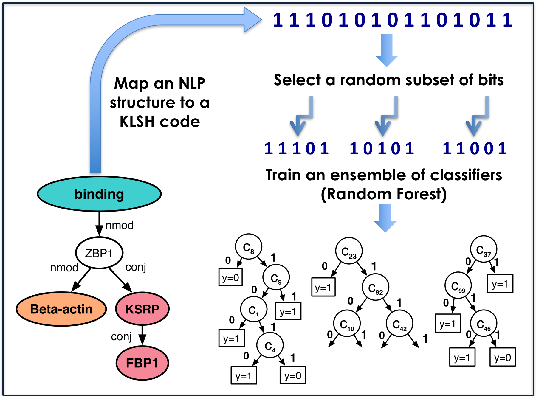
Figure 2: On the left, we show a subgraph from Fig. 1 which has to be classified (we assume binary classification). We map the subgraph to a high-dimensional, kernel similarity-based locality-sensitive hashcode ($\boldsymbol{c}$), and use it as a feature vector for an ensemble classifier. For instance, an efficient and intuitive approach is to train a Random Forest on binary kernel-hashcodes; in the figure, the nodes in a decision tree makes decisions simply based on hashcode bit values, where each bit represents presence or absence of some structural pattern in the subgraph.

2.1 Kernel Locality-Sensitive Hashing (KLSH)

Previously, Kernel Locality-Sensitive Hashing (KLSH) was used for constructing approximate kernelized k-Nearest Neighbor (kNN) graphs (?; ?). The key idea of KLSH as an approximate technique for finding the nearest neighbors of a data point is that rather than computing its similarity w.r.t. all other data points in a given set, the kernel similarity function is computed only w.r.t. the data points in the bucket of its hashcode (KLSH code). This approximation works well in practice if the hashing approach is locality sensitive, i.e. data points that are very similar to each other are assigned hashcodes with minimal Hamming distance to each other.

Herein, we brief on the generic procedure for mapping an arbitrary data point $S_{i}$ to a binary kernel-hashcode $\boldsymbol{c}_{i}\in\{0,1\}^{H}$, using a KLSH technique that relies upon the convolution kernel function $K(.,.;\boldsymbol{\theta})$.

Let us consider a set of data points $\boldsymbol{S}$ that might include both labeled and unlabeled examples. As a first step in constructing the KLSH codes, we select a random subset $\boldsymbol{S}^{R}\subset\boldsymbol{S}$ of size $|\boldsymbol{S}^{R}|=M$, which we call a reference set; this corresponds to the grey dots in the left-most panel of Fig. 3. Typically, the size of the reference set is significantly smaller than the size of the whole dataset, $M\ll N$.

Next, let $\boldsymbol{k}_{i}$ be a real-valued vector of size $M$, whose $j$–th component is the kernel similarity between the data point $S_{i}$ and the $j$–th element in the reference set, $k_{i,j}=K(S_{i},S^{R}_{j};\boldsymbol{\theta})$. Further, let $h_{l}(\boldsymbol{k}_{i})$, $l=1,\cdots,H$, be a set of $H$ binary valued hash functions that take $\boldsymbol{k}_{i}$ as an input and map it to binary bits and let $\boldsymbol{h}(\boldsymbol{k}_{i})=\{h_{l}(\boldsymbol{k_{i}})\}_{l=1}^{H}$. The kernel hashcode representation is then given as $\boldsymbol{c}_{i}=\boldsymbol{h}(\boldsymbol{k}_{i})$.

We now describe a specific choice of hash functions $h_{l}(.)$ based on nearest neighbors, called as Random k Nearest Neighbors (RkNN). For a given $l$, let $\boldsymbol{S}_{l}^{1}\subset\boldsymbol{S}^{R}$ and $\boldsymbol{S}_{l}^{2}\subset\boldsymbol{S}^{R}$ be two randomly selected, equal-sized and non-overlapping subsets of $\boldsymbol{S}^{R}$, $|\boldsymbol{S}_{l}^{1}|=|\boldsymbol{S}_{l}^{2}|=\alpha$, $\boldsymbol{S}_{l}^{1}\cap\boldsymbol{S}_{l}^{2}=\emptyset$. Those sets are indicated by red and blue dots in Fig. 3. Furthermore, let $k_{i,l}^{1}=\max_{S\in\boldsymbol{S}_{l}^{1}}K(S_{i},S)$ be the similarity between $S_{i}$ and its nearest neighbor in $\boldsymbol{S}_{l}^{1}$, with $k_{i,l}^{2}$ defined similarly (indicated by red and blue arrows in Fig. 3). Then the corresponding hash function is:

$$h_{l}(\boldsymbol{k}_{i})=\begin{cases}1,&\text{if }k_{i,l}^{1}<k_{i,l}^{2}\\ 0,&\text{otherwise}\end{cases}.$$ (1)

Pictorial illustration of this hashing scheme is provided in Fig. 3, where $S_{i}$’s nearest neighbors in either subset are indicated by the red and blue arrows.

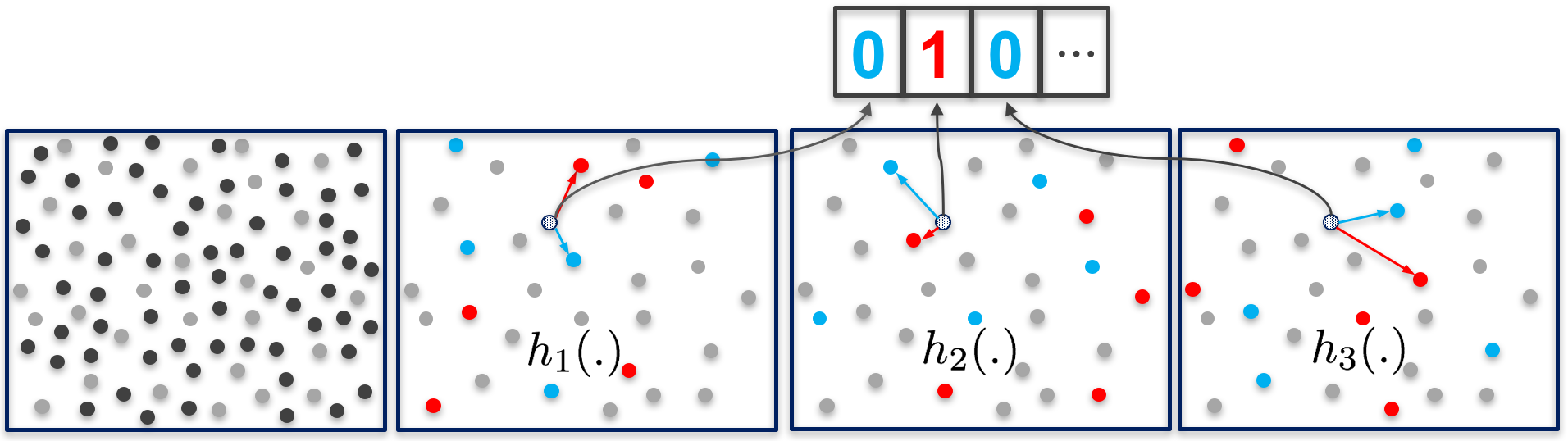
Figure 3: An illustration of the KLSH technique, Random K Nearest Neighbors (RkNN). First, we obtain a small subset (gray dots) from a super set of NLP structures as a reference set $\boldsymbol{S}^{R}$ that we use for constructing hash functions. For each hash function, two random subsets from the gray dots are obtained, denoted by red and blue. For a given structure, we find its kernel-based 1-nearest neighbor in both of the subsets as indicated by the arrows. Depending on which of the two 1-NNs–either the red 1-NN or the blue 1-NN—is the nearest to the sample, hash function $h_{1}(.)$ assigns value zero or one to the sample. The same procedure applies to $h_{2}(.)$ and $h_{3}(.)$. In this manner, we generate hashcodes with a large number of bits as explicit representations of NLP structures.

The same principle of random sub-sampling is applied in KLSH techniques previously proposed in (?; ?). In (?), $h_{l}(.)$ is built by learning a (random) maximum margin boundary (RMM) that discriminates between the two subsets, $\boldsymbol{S}^{1}_{l}$ and $\boldsymbol{S}^{2}_{l}$. In (?), $h_{l}(.)$ is obtained from $\boldsymbol{S}^{1}_{l}\cup\boldsymbol{S}^{2}_{l}$, which is a (approximately) random linear hyperplane in the kernel implied feature space; this is referred to as “Kulis” here.

In summary, we define klsh$(.;\boldsymbol{\theta},\boldsymbol{S}^{R})$ as the function, that is parameterized by $\boldsymbol{\theta}$ and $\boldsymbol{S}^{R}$, and maps a input data point $S_{i}$ to its KLSH code $\boldsymbol{c}_{i}$, using the kernel function $K(.,.;\boldsymbol{\theta})$ and the set of hash functions $\boldsymbol{h}(.)$ as subroutines.

$$\boldsymbol{c}_{i}=\text{klsh}(S_{i};\boldsymbol{\theta},\boldsymbol{S}^{R});\ \ \boldsymbol{c}_{i}=\boldsymbol{h}(\boldsymbol{k}_{i});\ \ k_{i,j}=K(S_{i},S^{R}_{j};\boldsymbol{\theta})$$ (2)

Next, in Sec. 3, we propose our approach of learning KLSH codes as generalized representations of NLP structures for classification problems.

3 KLSH for Representation Learning

We propose a novel use of KLSH where the hashcodes (KLSH codes) can serve as generalized representations (feature vectors) of the data points. Since the KLSH property of being locality sensitive (?) ensures the data points in the neighborhood of (or within the same) hashcode bucket are similar, hashcodes should serve as a good representation of the data points.

In contrast to the use of KLSH for k-NN, after obtaining the hashcodes for data points, we ignore the step of computing kernel similarities between data points in the neighboring buckets. In kNN classifiers using KLSH, a small number of hashcode bits ($H$), corresponding to a small number of hashcode buckets, generate a coarse partition of the feature space—sufficient for approximate computation of a kNN graph. In our representation learning framework, however, hashcodes must extract enough information about class labels from the data points, so we propose to generate longer hashcodes, i.e. $H\gg 1$. It is worthwhile noting that for a fixed number of kernel computations $M$ per structure $S_{i}$ ($|\boldsymbol{S}^{R}|=M$), a large number of hashcode bits ($H$) can be generated through the randomization principle with computational cost linear in $H$.

Unlike regular kernel methods (SVM, kNN, etc.), we use kernels to build an explicit feature space, via KLSH. Referring to Fig. 3, when using RkNN technique to obtain $\boldsymbol{c}_{i}$ for $S_{i}$, $l_{th}$ hashcode bit, $\boldsymbol{c}_{i,l}$, should correspond to finding a substructure in $S_{i}$, that should also be present in its 1-NN from either the set $\boldsymbol{S}^{1}_{l}$ or $\boldsymbol{S}^{2}_{l}$, depending on the bit value being $0$ or $1$. Thus, $\boldsymbol{c}_{i}$ represents finding important substructures in $S_{i}$ in relation to $\boldsymbol{S}^{R}$. The same should apply for the other KLSH techniques.

Random Subspaces of Kernel Hashcodes:

The next question is how to use the binary-valued representations for building a good classifier.

Intuitively, not all the bits may be matching across the hashcodes of NLP structures in training and test datasets; a single classifier learned on all the hashcode bits may overfit to a training dataset. This is especially relevant for bio-information extraction tasks where there is a high possibility of mismatch between training and test conditions (?; ?); for e.g., in biomedical literature, the mismatch can be due to high diversity of research topics, limited data annotations, variations in writing styles including aspects like hedging, etc. So we adopt the approach of building an ensemble of classifiers, with each one built on a random subspace of hashcodes (?; ?).

For building each classifier in an ensemble of $R$ classifiers, $\eta$ bits are selected randomly from $H\gg 1$ hash bits; for inference on a test NLP structure $S_{*}$, we take mean statistics over the inferred probability vectors from each of the classifiers, as it is a standard practice in ensemble approaches. Another way of building an ensemble from subspaces of hashcodes is bagging (?). If we use a decision tree as a classifier in ensemble, it corresponds to a random forest (?; ?).

It is highly efficient to train a random forest (RF) with a large number of decision trees ($R\gg 1$), even on long binary hashcodes ($H\gg 1$), leveraging the fact that decision trees can be very efficient to train and test on binary features.

3.1 Supervised Optimization of KLSH

In this section, we propose a framework for optimization of the KLSH codes as generalized representations for a supervised classification task. As described in Sec. 2.1, the mapping of a data points (an NLP structure $S$) to a KLSH code depends upon the kernel function $K(.,.;\boldsymbol{\theta})$ and the reference set $\boldsymbol{S}^{R}$ (Eq. 2). So, within this framework, we optimize the KLSH codes via learning the kernel parameters $\boldsymbol{\theta}$, and optionally the reference set $\boldsymbol{S}^{R}$. One important aspect of our optimization setting is that the parameters under optimization are shared between all the hash functions jointly, and are not specific to any of the hash functions.

Mutual Information as an Objective Function:

Intuitively, we want to generate KLSH codes that are maximally informative about the class labels. Thus, for optimizing the KLSH codes, a natural objective function is the mutual information (MI) between KLSH codes of $\boldsymbol{S}$ and the class labels, ${\mathcal{I}}(\boldsymbol{c}:y)$ (?).

$$\boldsymbol{\theta}^{*},{\boldsymbol{S}^{R}}^{*}\leftarrow\mathop{\arg\max}\limits_{\boldsymbol{\theta},\ \boldsymbol{S}^{R}:\boldsymbol{S}^{R}\subset\boldsymbol{S}}{\mathcal{I}}(\boldsymbol{c}:y);\ \boldsymbol{c}=\text{klsh}(S;\boldsymbol{\theta},\boldsymbol{S}^{R})$$ (3)

The advantage of MI as the objective, being a fundamental measure of dependence between random variables, is that it is generic enough for optimizing KLSH codes as generalized representations (feature vectors) of data points to be used with any classifier. Unfortunately, exact estimates of MI function in high-dimensional settings is an extremely difficult problem due to the curse of dimensionality, with the present estimators having very high sample complexity (?; ?; ?; ?; ?; ?; ?). Instead, here we propose to maximize a novel, computationally efficient, good approximation of the MI function.

Approximation of Mutual Information:

To derive the approximation, we express the mutual information function as, ${\mathcal{I}}(\boldsymbol{c}:y)={\mathcal{H}}(\boldsymbol{c})-{\mathcal{H}}(\boldsymbol{c}|y)$, with ${\mathcal{H}}(.)$ denoting the Shannon entropy. For binary classification, the expression simplifies to:

$${\mathcal{I}}(\boldsymbol{c}:y)={\mathcal{H}}(\boldsymbol{c})\!-\!p(y\!=\!0){\mathcal{H}}(\boldsymbol{c}|y\!=\!0)\!-\!p(y\!=\!1){\mathcal{H}}(\boldsymbol{c}|y\!=\!1).$$

To compute the mutual information, we need to efficiently compute joint entropy of KLSH code bits, ${\mathcal{H}}(\boldsymbol{c})$. We propose a good approximation of ${\mathcal{H}}(\boldsymbol{c})$, as described below; same applies for ${\mathcal{H}}(\boldsymbol{c}|y\!=\!0)$ and ${\mathcal{H}}(\boldsymbol{c}|y\!=\!1)$.

$${\mathcal{H}}(\boldsymbol{c})=\sum_{l=1}^{H}{\mathcal{H}}(c_{l})\!-\!\mathcal{TC}(\boldsymbol{c})\approx\sum_{l=1}^{H}{\mathcal{H}}(c_{l})\!-\!\mathcal{TC}(\boldsymbol{c};\boldsymbol{z^{*}});$$ (4)

$${\mathcal{T}}{\mathcal{C}}(\boldsymbol{c};\boldsymbol{z})={\mathcal{T}}{\mathcal{C}}(\boldsymbol{c})-{\mathcal{T}}{\mathcal{C}}(\boldsymbol{c}|\boldsymbol{z}).$$ (5)

In Eq. 4, the first term is the sum of marginal entropies for the KLSH code bits. Marginal entropies for binary variables can be computed efficiently. Now, let us understand how to compute the second term in the approximation (Eq. 4). Herein, ${\mathcal{T}}{\mathcal{C}}(\boldsymbol{c};\boldsymbol{z})$ describes the amount of Total Correlations (Multi-variate Mutual Information)  within $\boldsymbol{c}$ that can be explained by a latent variables representation $\boldsymbol{z}$.

$$\boldsymbol{z^{*}}\leftarrow\mathop{\arg\max}\limits_{\boldsymbol{z}:|\boldsymbol{z}|=|\boldsymbol{c}|}{\mathcal{T}}{\mathcal{C}}(\boldsymbol{c};\boldsymbol{z})$$ (6)

An interesting aspect of the quantity $\mathcal{TC}(\boldsymbol{c};\boldsymbol{z})$ is that one can compute it efficiently for optimized $\boldsymbol{z^{*}}$ that explains maximum possible Total Correlations present in $\boldsymbol{c}$, s.t. $\mathcal{TC}(\boldsymbol{c}|\boldsymbol{z})\approx 0$. In (?), an unsupervised algorithm called CorEx  is proposed for obtaining such latent variables representation. Their algorithm is efficient for binary input variables, demonstrating a low sample complexity even in very high dimensions of input variables. Therefore it is particularly relevant for computing the proposed joint entropy approximation on hashcodes. For practical purposes, the dimension of latent representation $\boldsymbol{z}$ can be kept much smaller than the dimension of KLSH codes, i.e. $|\boldsymbol{z}|\ll H$. This helps to reduce the cost for computing the proposed MI approximation to negligible during the optimization (Eq. 3).

Denoting the joint entropy approximation as $\bar{{\mathcal{H}}}(\boldsymbol{c})$, we express the approximation of the mutual information as:

$$\bar{{\mathcal{I}}}(\boldsymbol{c}:y)=\bar{{\mathcal{H}}}(\boldsymbol{c})\!-\!p(y\!=\!0)\bar{{\mathcal{H}}}(\boldsymbol{c}|y\!=\!0)\!-\!p(y\!=\!1)\bar{{\mathcal{H}}}(\boldsymbol{c}|y\!=\!1).$$

For computation efficiency as well as robustness w.r.t. overfitting, we use small random subsets (of size $\gamma$) from a training set for stochastic empirical estimates of $\bar{{\mathcal{I}}}(\boldsymbol{c}:y)$, motivated by the idea of stochastic gradients (?). For a slight abuse of notation, when obtaining an empirical estimate of $\bar{{\mathcal{I}}}(\boldsymbol{c}:y)$ using samples set $\{\boldsymbol{C},\boldsymbol{y}\}$, we simply denote the estimate as: $\bar{{\mathcal{I}}}(\boldsymbol{C}:\boldsymbol{y})$. Here it is also interesting to note that computation of $\bar{{\mathcal{I}}}(\boldsymbol{c}:y)$ is very easy to parallelize since the kernel matrices and hash functions can be computed in parallel.

It is worth noting that in our proposed approximation of the MI, both terms need to be computed. In contrast, in the previously proposed variational lower bounds for MI (?; ?; ?), MI is expressed as, ${\mathcal{I}}(\boldsymbol{c}:y)={\mathcal{H}}(y)-{\mathcal{H}}(y|\boldsymbol{c})$, so as to obtain a lower bound simply by upper bounding the conditional entropy term with a cross entropy term while ignoring the first term as a constant. Clearly, these approaches are not using MI in its true sense, rather using conditional entropy (or cross entropy) as the objective. Further, our approximation of MI also allows semi-supervised learning as the first term is computable even for hashcodes of unlabeled examples.

Algorithm 1 Optimizing Reference Set for KLSH

0:  Train dataset, $\{\boldsymbol{S},\boldsymbol{y}\}$; size of the reference set, $M$; $\beta,\gamma$ are number of samples from $\boldsymbol{S}$, as candidates for $\boldsymbol{S}^{R}$, and for computing the objective, respectively.

1:  $\boldsymbol{S}^{R}$ $\leftarrow$ randomSubset($\boldsymbol{S}$, $M$) % $M$ samples from $\boldsymbol{S}$

2:   % optimizing the reference set up to size $M$ greedily

3:  for $j=1\to M$ do

4:     $\boldsymbol{S}^{eo},\boldsymbol{y}^{eo}\leftarrow$ randomSubset($\{\boldsymbol{S},\boldsymbol{y}\},\gamma$) %  $\gamma$ samples from $\boldsymbol{S}$ for estimating the objective $\bar{{\mathcal{I}}}(.)$.

5:     $\boldsymbol{S}^{cr}$ $\leftarrow$ randomSubset($\boldsymbol{S}$, $\beta$) % $\beta$ samples from $\boldsymbol{S}$ as choices for selection to $\boldsymbol{S}^{R}$

6:      % iterate over candidates elements for greedy step

7:     for $q=1\to\beta$ do

8:        $S^{R}_{j}\leftarrow S^{cr}_{q}$ % $S^{cr}_{q}$ is a choice for selection to $\boldsymbol{S}^{R}$

9:        $\boldsymbol{c}^{eo}_{i}\leftarrow$ klsh($S^{eo}_{i}$; $\boldsymbol{\theta}$, $\boldsymbol{S}^{R}$) $\forall{S^{eo}_{i}\in\boldsymbol{S}^{eo}}$ % Eq. 2

10:        $\boldsymbol{mi}_{q}\leftarrow$ $\bar{{\mathcal{I}}}$($\boldsymbol{C}^{eo},\boldsymbol{y}^{eo}$) % estimating objective

11:     end for

12:     $S^{R}_{j}\leftarrow$ chooseElementWithMaxMI($\boldsymbol{mi}$, $\boldsymbol{S}^{cr}$)

13:  end for

14:  return  $\boldsymbol{S}^{R}$

Algorithms for Optimization:

Using the proposed approximate mutual information function as an objective, one can optimize the kernel parameters either using grid search or an MCMC procedure.

For optimizing the reference set $\boldsymbol{S}^{R}$ (of size $M$) as a subset of $\boldsymbol{S}$, via maximization of the same objective, we propose a greedy algorithm with pseudo code in Alg. 1. Initially, $\boldsymbol{S}^{R}$ is initialized with a random subset of $\boldsymbol{S}$ (line 1). Thereafter, $\bar{{\mathcal{I}}}(.)$ is maximized greedily, updating one element in $\boldsymbol{S}^{R}$ in each greedy step (line 3); greedy maximization of MI-like objectives has been successful (?; ?). Employing the paradigm of stochastic sampling, for estimating $\bar{{\mathcal{I}}}(.)$, we randomly sample a small subset of $\boldsymbol{S}$ (of size $\gamma$) along with their class labels (line 4). Also, in a single greedy step, we consider only a small random subset of $\boldsymbol{S}$ (of size $\beta$) as candidates for selection into $\boldsymbol{S}^{R}$ (line 5); for $\beta\gg 1$, with high probability, each element in $\boldsymbol{S}$ should be seen as a candidate at least once by the algorithm. Alg. 1 requires kernel computations of order, $O(\gamma M^{2}+\gamma\beta M)$, with $\beta,\gamma$ being the sampling size constants; in practice, $M\ll N$. Note that $\boldsymbol{\theta}$ and $\boldsymbol{S}^{R}$ can be optimized in an iterative manner.

3.2 Nonstationary Extension for Kernels

One common principle applicable to all the convolution kernel functions, $K(.,.)$, defining similarity between any two NLP structures is: $K(.,.)$ is expressed in terms of a kernel function, $k(.,.)$, that defines similarity between any two tokens (node/edge labels in Fig. 1). Some common examples of $k(.,.)$, from previous works (?; ?), are:

$$\text{Gaussian: }k(a,b)=\exp(-||\boldsymbol{w}_{a}-\boldsymbol{w}_{j}||_{b}^{2}),$$

$$\text{Sigmoid: }k(a,b)=(1+\tanh(\boldsymbol{w}_{a}^{T}\boldsymbol{w}_{b}))/2.$$

Herein, $a,b$ are tokens, and $\boldsymbol{w}_{a}$, $\boldsymbol{w}_{b}$ are the corresponding word vectors. The first kernels is stationary, i.e. translation invariant (?), and the second one is nonstationary, although lacking nonstationarity-specific parameters for learning nonstationarity in a data-driven manner.

There are generic nonstationarity-based parameterizations, unexplored in NLP, applicable for extending any kernel, $k(.,.)$, to a nonstationary one, $k^{NS}(.,.)$, so as to achieve higher expressiveness and generalization in model learning (?; ?). For NLP, nonstationarity of $K(.,.)$ can be formalized as in Theorem 1; see the longer version of this paper for a proof.

Theorem 1.

A convolution kernel $K(.,.)$, that is a function of the kernel $k(.,.)$, is stationary if $k(.,.)$ is stationary, and vice versa. From a non-stationary $k^{NS}(.,.)$, the corresponding extension of $K(.,.)$, $K^{NS}(.,.)$, is also guaranteed to be a valid non-stationary convolution kernel.

One simple and intuitive nonstationary extension of $k(.,.)$ is: $k^{NS}(a,b)=\sigma_{a}k(a,b)\sigma_{b}$. Here, $\sigma\geq 0$, are nonstationarity-based parameters; for more details, see (?); another choice for the nonstationary extension is based on the concept of process convolution, as proposed in (?). If $\sigma_{a}=0$, it means that the token $a$ should be completely ignored when computing a convolution kernel similarity of an NLP structure (tree, path, etc.) that contains the token $a$ (node or edge label $a$) w.r.t. another NLP structure. Thus, the additional nonstationary parameters allow convolution kernels to be expressive enough for deciding if some substructures in an NLP structure should be ignored explicitly.

Models	(AIMed, BioInfer)	(BioInfer, AIMed)
SVM1 (?)	0.25	0.44
SVM2 (?)	0.47	0.47
SVM (?)	0.53	0.50
SVM (?)	0.41	0.42
	(0.67, 0.29)	(0.27, 0.87)
CNN (?)	0.37	0.45
Bi-LSTM (?)	0.30	0.47
CNN (?)	0.48	0.50
	(0.40, 0.61)	(0.40, 0.66)
RNN (?)	0.49	0.51
CNN-RevGrad (?)	0.43	0.47
Bi-LSTM-RevGrad (?)	0.40	0.46
Adv-CNN (?)	0.54	0.49
Adv-Bi-LSTM (?)	$\boldsymbol{0.57}$	0.49
KLSH-kNN	$0.51$	$0.51$
	(0.41, 0.68)	(0.38, 0.80)
KLSH-RF	$\boldsymbol{0.57}$	$\boldsymbol{0.54}$
	(0.46, 0.75)	(0.37, 0.95)

Table 1: Cross-corpus evaluation results for (training, test) pairs of PPI datasets, AIMed and BioInfer datasets. For each model, we report F1 score in the first row corresponding to it. In some of the previous works, precision, recall numbers are not reported; wherever available, we show precision, recall numbers as well, in brackets.

While the above proposed idea of nonstationary kernel extensions for NLP structures remains general, for the experiments, the nonstationary kernel for similarity between tuples with format (edge-label, node-label) is defined as the product of kernels on edge labels, $e_{a},e_{b}$, and node labels, $n_{a},n_{b}$,

$$k^{NS}\!((e_{i},n_{i}),\!(e_{j},n_{j}))=\sigma_{e_{i}}k_{e}(e_{i},e_{j})\sigma_{e_{j}}k_{n}(n_{i},n_{j}),$$

with $\sigma$ operating only on edge labels. Edge labels come from syntactic or semantic parses of text with small size vocabulary (see syntactic parse-based edge labels in Fig. 1); we keep $\sigma\in\{0,1\}$ as a measure for robustness to over-fitting. These parameters are learned by maximizing the same objective, $\bar{{\mathcal{I}}}(.)$, using the well known Metropolis-Hastings MCMC procedure (?).

4 Experiments

We evaluate our model “KLSH-RF” (kernelized locality-sensitive hashing with random forest) for the biomedical relation extraction task using four public datasets, AIMed, BioInfer, PubMed45, BioNLP, as briefed below. Fig. 1 illustrates that the task is formulated as a binary classification of extraction candidates. For evaluation, it is standard practice to compute precision, recall, and F1 score on the positive class (i.e., identifying valid extractions).

Details on Datasets and Structural Features:

AIMed and BioInfer: For AIMed and BioInfer datasets, cross-corpus evaluation has been performed in many previous works (?; ?; ?; ?). Herein, the task is of identifying pairs of interacting proteins (PPI) in a sentence while ignoring the interaction type. We follow the same evaluation setup, using Stanford Dependency Graph parses of text sentences to obtain undirected shortest paths as structural features for use with a path kernel (PK) to classify protein-protein pairs.

PubMed45 & BioNLP: We use PubMed45 and BioNLP datasets for an extensive evaluation of our KLSH-RF model; for more details on the two datasets, see (?) and (?; ?; ?). Annotations in these datasets are richer in the sense that a bio-molecular interaction can involve up to two participants, along with an optional catalyst, and an interaction type from an unrestricted list. In PubMed45 (BioNLP) dataset, 36% (17%) of the “valid” interactions are such that an interaction must involve two participants and a catalyst. For both datasets, we use abstract meaning representation (AMR) to build subgraph or shortest path-based structural features (?), for use with graph kernels (GK) or path kernels (PK) respectively, as done in the recent works evaluating these datasets (?; ?). For a fair comparison of the classification models, we use the same bio-AMR parser (?) as in the previous works. In (?), the PubMed45 dataset is split into 11 subsets for evaluation, at paper level. Keeping one of the subsets for testing, we use the others for training a binary classifier. This procedure is repeated for all 11 subsets in order to obtain the final F1 scores (mean and standard deviation values are reported from the numbers for 11 subsets). For BioNLP dataset (?; ?; ?), we use training datasets from years 2009, 2011, 2013 for learning a model, and the development dataset from year 2013 as the test set; the same evaluation setup is followed in (?).

Models	PubMed45	PubMed45-ERN	BioNLP
SVM (?)	$0.45$$\pm$$0.25$	$0.33$$\pm$$0.16$	$0.46$
	(0.58, 0.43)	(0.33, 0.45)	(0.35, 0.67)
LSTM (?)	N.A.	N.A.	0.46
			(0.51, 0.44)
LSTM	$0.30$$\pm$$0.21$	$0.29$$\pm$$0.14$	0.59
	(0.38, 0.28)	(0.42, 0.33)	(0.89, 0.44)
Bi-LSTM	$0.46$$\pm$$0.26$	$0.37$$\pm$$0.15$	0.55
	(0.59, 0.43)	(0.45, 0.40)	(0.92, 0.39)
LSTM-CNN	$0.50$$\pm$$0.27$	$0.31$$\pm$$0.17$	0.60
	(0.55, 0.50)	(0.35, 0.40)	(0.77, 0.49)
CNN	$0.51$$\pm$$0.28$	$0.33$$\pm$$0.18$	0.60
	(0.46, 0.46)	(0.36, 0.32)	(0.80, 0.48)
KLSH-kNN	$0.46$$\pm$$0.21$	$0.23$$\pm$$0.13$	$0.60$
	(0.44, 0.53)	(0.23, 0.29)	(0.63, 0.57)
KLSH-RF	$\boldsymbol{0.57}$$\pm$$\boldsymbol{0.25}$	$\boldsymbol{0.45}$$\pm$$\boldsymbol{0.22}$	$\boldsymbol{0.63}$
	(0.63, 0.55)	(0.51, 0.52)	(0.78, 0.53)

Table 2: Evaluation results for PubMed45 and BioNLP datasets. For each model, we report F1 score (mean $\pm$ standard deviation) in the first row corresponding to it, and show mean-precision, mean-recall numbers as well, in brackets. For BioNLP, we don’t show standard deviation since there is only one fixed test subset.

In addition to the models previously evaluated on these datasets, we also compare our KLSH-RF model to KLSH-kNN (kNN classifier with KSLH approximation).

For PubMed45 and BioNLP datasets, for the lack of evaluations of previous works on these datasets, we perform extensive empirical evaluation ourselves of competitive neural network models, LSTM, Bi-LSTM, LSTM-CNN, CNN; from fine-grained tuning, for PubMed45 & PubMed45-ERN datasets, the tuned neural architecture was a five-layer network, [8, 16, 32, 16, 8], having 8, 16, 32, 16, and 8 nodes, respectively, in the 1st, 2nd, 3rd, 4th, 5th hidden layers; for BioNLP dataset, the tuned neural architecture was a two layer network, [32, 32].

Parameter Settings:

We use GK and PK, both using the same word vectors, with kernel parameter settings same as in (?; ?).

Reference set size, $M$, doesn’t need tuning in our proposed model; there is a trade-off between compute cost and accuracy; by default, we keep $M=100$. For tuning any other parameters in our model or competitive models, including the choice of a kernel similarity function (PK or GK), we use 10% of training data, sampled randomly, for validation purposes. From a preliminary tuning, we set parameters, $H=1000$, $R=250$, $\eta=30$, $\alpha=2$, and choose RMM as the KLSH technique from the three choices discussed in Sec. 2.1; same parameter values are used across all the experiments unless mentioned otherwise.

When selecting reference set $\boldsymbol{S}^{R}$ randomly, we perform 10 trials, and report mean statistics. (Variance across these trials is small, empirically.) The same applies for KLSH-kNN. When optimizing $\boldsymbol{S}^{R}$ with Alg. 1, we use $\beta$$=$$1000$, $\gamma$$=$$300$ (sampling parameters are easy to tune). We employ 4 cores on an i7 processor, with 16GB memory.

4.1 Main Results for KLSH-RF

In the following we compare the simplest version of our KLSH-RF model that is optimized by learning the kernel parameters via maximization of the MI approximation, as described in Sec. 3.1 ($\gamma=1000$). In summary, our KLSH-RF model outperforms state-of-the-art models consistently across the four datasets, along with very significant speedups in training time w.r.t. traditional kernel classifiers.

Results for AIMed and BioInfer Datasets:

In reference to Tab. 1, KLSH-RF gives an F1 score significantly higher than state-of-the-art kernel-based models (6 pts gain in F1 score w.r.t. KLSH-kNN), and consistently outperforms the neural models. When using AIMed for training and BioInfer for testing, there is a tie between Adv-Bi-LSTM (?) and KLSH-RF. However, KLSH-RF still outperforms their Adv-CNN model by 3 pts; further, the performance of Adv-CNN and Adv-Bi-LSTM is not consistent, giving a low F1 score when training on the BioInfer dataset for testing on AIMed. For the latter setting of AIMed as a test set, we obtain an F1 score improvement by 3 pts w.r.t. the best competitive models, RNN & KLSH-kNN. Overall, the performance of KLSH-RF is more consistent across the two evaluation settings, in comparison to any other competitive model.

The models based on adversarial neural networks (?; ?), Adv-CNN, Adv-Bi-LSTM, CNN-RevGrad, Bi-LSTM-RevGrad, are learned jointly on labeled training datasets and unlabeled test sets, whereas our model is purely supervised. In contrast to our principled approach, there are also system-level solutions using multiple parses jointly, along with multiple kernels, and knowledge bases (?; ?). We refrain from comparing KLSH-RF w.r.t. such system level solutions, as it would be an unfair comparison from a modeling perspective.

Results for PubMed45 and BioNLP Datasets:

A summary of main results is presented in Tab. 2. “PubMed45-ERN” is another version of the PubMed45 dataset from (?), with ERN referring to entity recognition noise. Clearly, our model gives F1 scores significantly higher than SVM, LSTM, Bi-LSTM, LSTM-CNN, CNN, and KLSH-kNN model. For PubMed45, PubMed45-ERN, and BioNLP, the F1 score for KLSH-RF is higher by 6 pts, 8 pts, and 3 pts respectively w.r.t. state of the art; KLSH-RF is the most consistent in its performance across the datasets and significantly more scalable than SVM. Note that standard deviations of F1 scores are high for the PubMed45 dataset (and PubMed45-ERN) because of the high variation in distribution of text across the 11 test subsets (the F1 score improvements with our model are statistically significant, p-value=4.4e-8).

For the PubMed45 dataset, there are no previously published results with a neural model (LSTM). The LSTM model of (?), proposed specifically for the BioNLP dataset, is not directly applicable for the PubMed45 dataset because the list of interaction types in the latter is unrestricted. F1 score numbers for SVM classifier were also improved in (?) by additional contributions such as document-level inference, and the joint use of semantic and syntactic representations; those system-level contributions are complementary to ours, so excluded from the comparison.

4.2 Detailed Analysis of KLSH-RF

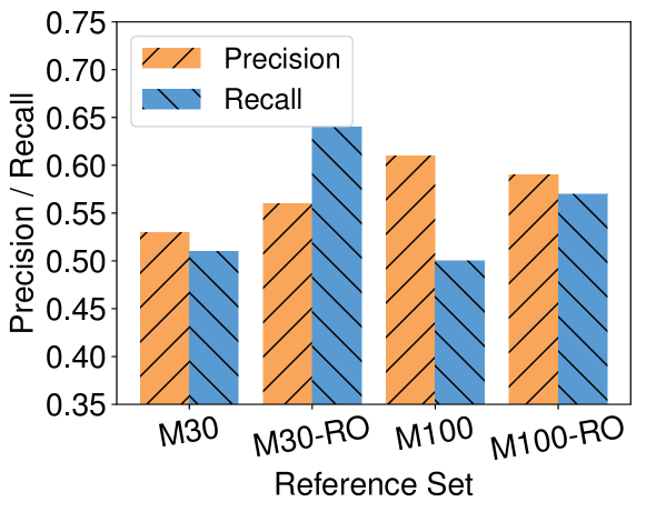
(a) Reference Set Opt. (PubMed45)

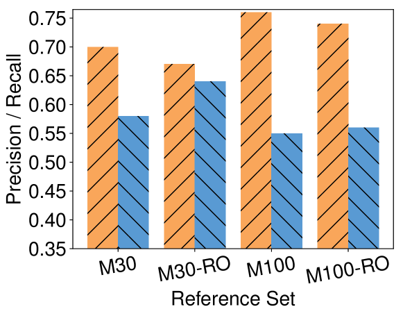
(b) Reference Set Opt. (BioNLP)

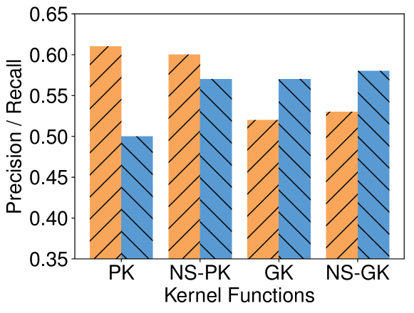
(c) NSK Learning (PubMed45)

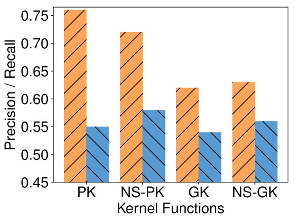
(d) NSK Learning (BioNLP)

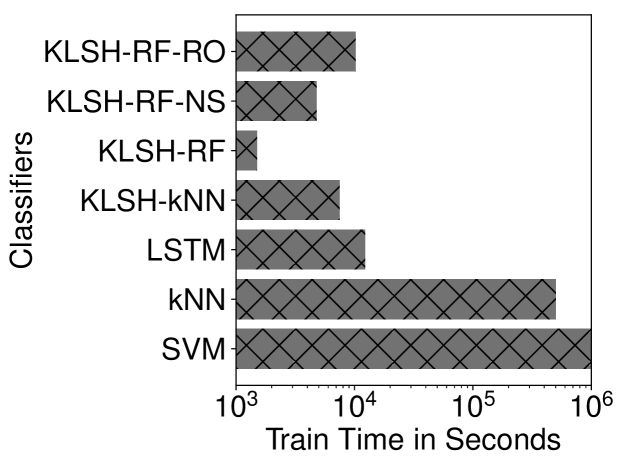
(e) Training Time (BioNLP)

Figure 4: Detailed Evaluation of KLSH-RF model, using PubMed45 and BioNLP datasets. Here, orange and blue bars are for precision and recall numbers respectively. “NSK” refers to nonstationary kernel learning; PK & GK denote Path Kernels and Graph Kernels respectively; NS-PK and NS-GK are extensions of PK and GK respectively, with addition of nonstationarity based binary parameters; “M30” represents $\boldsymbol{S}^{R}$ of size $30$ selected randomly, and the suffix “RO” in “M30-RO” refers to optimization of $\boldsymbol{S}^{R}$ (Reference optimization) in contrast to random selection of $\boldsymbol{S}^{R}$.

While we are able to obtain superior results with our basic KLSH-RF model w.r.t. state-of-the-art methods using just core optimization of the kernel parameters $\boldsymbol{\theta}$, in this subsection we analyze how we can further improve the model. In Fig. 4 we present our results from optimization of other aspects of the KLSH-RF model: reference set optimization (RO) and non-stationary kernel parameters learning (NS). (In the longer version of this paper, we also analyze the effect of parameters, $H,R$, and the choice of KLSH technique, under controller experiment settings.) We report mean values for precision, recall, F1 scores. For these experiments, we focus on PubMed45 and BioNLP datasets.

Reference Set Optimization:

In Fig. 4(a) and 4(b), we analyze the effect of the reference set optimization (RO), in comparison to random selection, and find that the optimization leads to significant increase in recall (7-13 pts) for PubMed dataset along with a marginal increase/decrease in precision (2-3 pts); we used PK for these experiments. For the BioNLP dataset, the improvements are not as significant. Further, as expected, the improvement is more prominent for smaller size of reference set ($M$). To optimize reference set $\boldsymbol{S}^{R}$ for $M=100$, it takes approximately 2 to 3 hours (with $\beta=1000,\gamma=300$ in Alg. 1).

Nonstationary Kernel Learning (NSK):

In Fig. 4(c) and 4(d), we compare performance of non-stationary kernels, w.r.t. traditional stationary kernels (M=100). As proposed in Sec. 3.2, the idea is to extend a convolution kernel (PK or GK) with non-stationarity-based binary parameters (NS-PK or NS-GK), optimized using our MCMC procedure via maximizing the proposed MI approximation based objective ($\gamma=300$). For the PubMed45 dataset with PK, the advantage of NSK learning is more prominent, leading to high increase in recall (7 pts), and a very small drop in precision (1 pt). Compute time for learning the non-stationarity parameters in our KLSH-RF model is less than an hour.

Compute Time:

Compute times to train all the models are reported in Fig. 4(e) for the BioNLP dataset; similar time scales apply for other datasets. We observe that our basic KLSH-RF model has a very low training cost, w.r.t. models like LSTM, KLSH-kNN, etc. (similar analysis applies for inference cost). The extensions of KLSH-RF, KLSH-RF-RO and KLSH-RF-NS, are more expensive yet cheaper than LSTM and SVM.

5 Related Work

Besides some related work mentioned in the previous sections, this section focuses on relevant state-of-the-art literature in more details.

Other Hashing Techniques:

In addition to hashing techniques considered in this paper, other locality-sensitive hashing techniques (?; ?; ?) are either not kernel based, or they are defined for specific kernels that are not applicable for hashing of NLP structures (?). In deep learning, hashcodes are used for similarity search but classification of objects (?).

Hashcodes for Feature Compression:

Binary hashing (not KLSH) has been used as an approximate feature compression technique in order to reduce memory and computing costs  (?; ?). Unlike prior approaches, this work proposes to use hashing as a representation learning (feature extraction) technique.

Using Hashcodes in NLP:

In NLP, hashcodes were used only for similarity or nearest neighbor search for words/tokens in various NLP tasks (?; ?; ?); our work is the first to explore kernel-hashing of various NLP structures, rather than just tokens.

Weighting Substructures:

Our idea of skipping substructures, due to our principled approach of nonstationary kernels, is somewhat similar to sub-structure mining algorithms (?; ?). Learning the weights of sub-structures was recently proposed for regression problems, but not yet for classification (?).

Kernel Approximations:

Besides the proposed model, there are other kernel-based scalable techniques in the literature, which rely on approximation of a kernel matrix or a kernel function (?; ?; ?; ?; ?; ?; ?). However, those approaches are only used as computationally efficient approximations of the traditional, computationally-expensive kernel-based classifiers; unlike those approaches, our method is not only computationally more efficient but also yields considerable accuracy improvements.

Nonstationary Kernels:

Nonstationary kernels have been explored for modeling spatio-temporal environmental dynamics or time series relevant to health care, finance, etc, though expensive to learn due to a prohibitively large number of latent variables (?; ?; ?). Ours is the first work proposing nonstationary convolution kernels for natural language modeling; the number of parameters is constant in our formulation, so highly efficient in contrast to the previous works.

6 Conclusions

In this paper we propose to use a well-known technique, kernelized locality-sensitive hashing (KLSH), in order to derive feature vectors from natural language structures. More specifically, we propose to use random subspaces of KLSH codes for building a random forest of decision trees. We find this methodology particularly suitable for modeling natural language structures in supervised settings where there are significant mismatches between the training and the test conditions. Moreover we optimize a KLSH model in the context of classification performed using a random forest, by maximizing an approximation of the mutual information between the KLSH codes (feature vectors) and the class labels. We apply the proposed approach to the difficult task of extracting information about bio-molecular interactions from the semantic or syntactic parsing of scientific papers. Experiments on a wide range of datasets demonstrate the considerable advantages of our method.

7 Acknowledgments

This work was sponsored by the DARPA Big Mechanism program (W911NF-14-1-0364). It is our pleasure to acknowledge fruitful discussions with Karen Hambardzumyan, Hrant Khachatrian, David Kale, Kevin Knight, Daniel Marcu, Shrikanth Narayanan, Michael Pust, Kyle Reing, Xiang Ren, and Gaurav Sukhatme. We are also grateful to anonymous reviewers for their valuable feedback.

Appendix A Dataset Statistics

The number of valid/invalid extractions in each dataset is shown in Tab. 3.

Datasets	No. of Valid Extractions	No. of Invalid Extractions
PubMed45	2,794	20,102
BioNLP	6,527	34,958
AIMed	1,000	4,834
BioInfer	2,534	7,132

Table 3: Dataset statistics: number of “valid” & “invalid” extractions in each of the four datasets.

Appendix B Nonstationarity of Convolution Kernels for NLP

Definition 1 (Stationary kernel (?)).

A stationary kernel, between vectors $\boldsymbol{x}_{i},\boldsymbol{x}_{j}\in\mathbb{R}^{d}$, is the one which is translation invariant:

$$k(\boldsymbol{x}_{i},\boldsymbol{x}_{j})=k^{S}(\boldsymbol{x}_{i}-\boldsymbol{x}_{j}),$$

that means, it depends only upon the lag vector between $\boldsymbol{x}_{i}$ and $\boldsymbol{x}_{j}$, and not the data points themselves.

For NLP context, stationarity in convolution kernels is formalized as follows.

Theorem 2.

A convolution kernel $K(.,.)$, a function of the kernel $k(.,.)$, is stationary if $k(.,.)$ is stationary. From a nonstationary $k^{NS}(.,.)$, the corresponding extension of $K(.,.)$, $K^{NS}(.,.)$, is also guaranteed to be a valid nonstationary convolution kernel.

Proof.

Suppose we have a vocabulary set, $\{l_{1},\cdots,l_{p},\cdots,l_{2p}\}$, and we randomly generate a set of discrete structures $\mathcal{X}=\{X_{1},\cdots,X_{N}\}$, using $l_{1},\cdots,l_{p}$. For kernel $k(.,.)$, that defines similarity between a pair of labels, consider a case of stationarity, $k(l_{i},l_{j})=k(l_{i+p},l_{j})=k(l_{i},l_{j+p});i,j\in\{1,\cdots,p\}$, where its value is invariant w.r.t. to the translation of a label $l_{i}$ to $l_{i+p}$. In the structures, replacing labels $l_{1},\cdots,l_{p}$ with $l_{p+1},\cdots,l_{2p}$ respectively, we obtain a set of new structures $\bar{\mathcal{X}}=\{\bar{X}_{1},\cdots,\bar{X}_{N}\}$. Using a convolution kernel $K(.,.)$, as a function of $k(.,.)$, we obtain same (kernel) Gram matrix on the set $\bar{\mathcal{S}}$ as for $\mathcal{S}$. Thus $K(.,.)$ is also invariant w.r.t. the translation of structures set $\mathcal{S}$ to $\mathcal{\bar{S}}$, hence a stationary kernel (Def. 1). For establishing the nonstationarity property, following the above logic, if using $K^{NS}(.,.)$, we obtain a (kernel) Gram matrix on the set $\bar{\mathcal{S}}$ that is different from the set $\mathcal{S}$. Therefore $K^{NS}(.,.)$ is not invariant w.r.t. the translation of set $\mathcal{S}$ to $\mathcal{\bar{S}}$, hence a nonstationary kernel (Def. 1). ∎

Appendix C Brief on MCMC Procedure for Optimizing Nonstationary Parameters

Denoting all the nonstationary parameters as $\boldsymbol{\sigma}$, we set $\boldsymbol{\sigma}=\boldsymbol{1}$ as the first sample of MCMC. Now, for producing a new sample $\boldsymbol{\sigma}^{\prime}$ from current sample $\boldsymbol{\sigma}$ in the Markov chain, we randomly pick one of the parameters and flip its binary value from 0 to 1 or vica versa. This new sample is accepted with probability: $A(\boldsymbol{\sigma},\boldsymbol{\sigma}^{\prime})=\min\left(1,\exp\left({\mathcal{I}}(\boldsymbol{C}^{\prime}:\boldsymbol{y})\right)/\exp\left({\mathcal{I}}(\boldsymbol{C}:\boldsymbol{y})\right)\right)$, with hashcodes $\boldsymbol{C}^{\prime}$ and $\boldsymbol{C}$ computed using the kernel parameters samples $\boldsymbol{\sigma}^{\prime}$ & $\boldsymbol{\sigma}$, respectively. This procedure is performed for a fixed number of samples, and then the MCMC sample with highest $\bar{{\mathcal{I}}}(.:.)$ is accepted.

Appendix D More Experiments

Analyzing Hashing Parameters

In Fig. 5(a) and 5(b), we compare performance of all the three KLSH techniques with our model. For these experiments, $\alpha$ is fixed to value $2$. We found that Kulis is highly sensitive to the value of $\alpha$ in contrast to RMM and RkNN; accuracy numbers drop with Kulis for higher value of $\alpha$ (those results are not shown here).

For PubMed45 dataset, we also vary the parameters $R,H$ ($\eta$=None & $M=500$, using PK). As we mentioned previously, for obtaining random subspaces of kernel-hashcodes, we can either use bagging ($\eta$=None), i.e. the random subset of training dataset (with resampling), or explicitly take a random subset of hashcode bits ($\eta=30$). Here, in Fig. 5(c) and Fig. 5(d), we present results for both approaches, as two types of our KLSH-RF model, with PK. We can see that the gain in accuracy, is marginal, with an increase in the number of decision trees, after a minimal threshold. For a low value of $H$ (15, 30), the F1 score drops significantly. In 5(c), we decrease $H$ down to value 100 only since the number of sampled hashcode bits ($\eta$) is 30. We also note that despite the high number of hashcode bits, classification accuracy improves only if we have a minimal number of decision trees.

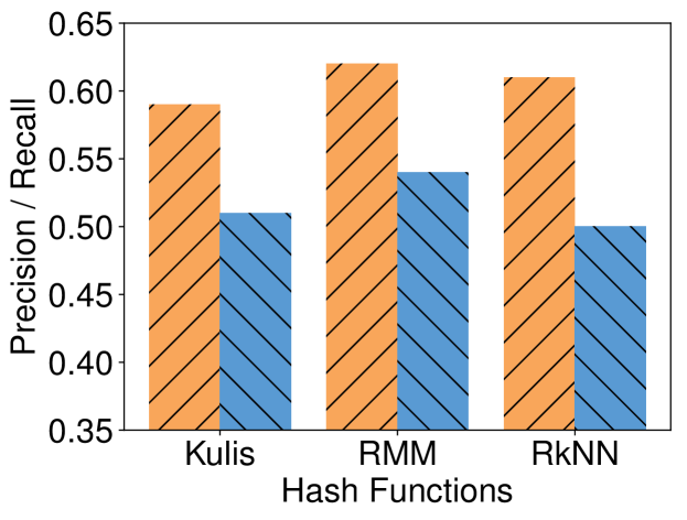
(a) Hash Functions (PubMed45)

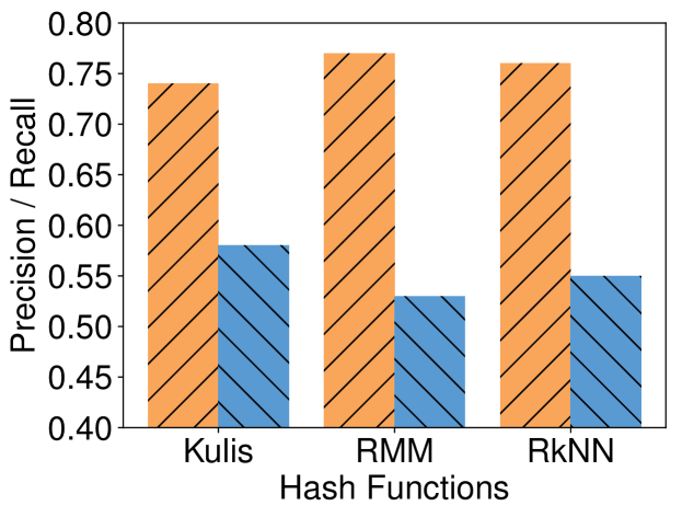
(b) Hash Functions (BioNLP)

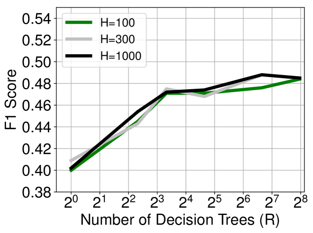
(c) PubMed45- Sampling features

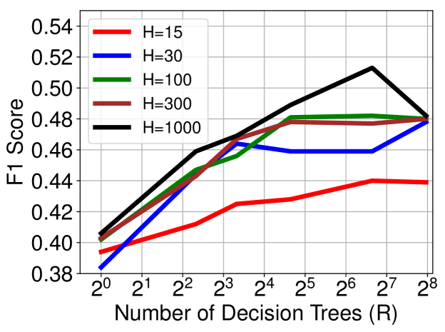
(d) Varying $H,R$ (PubMed45)

Figure 5: Detailed Empirical Analysis of KLSH-RF model, using PubMed45 and BioNLP datasets. Here, orange and blue bars are for precision and recall numbers respectively.

Appendix E Convolution Kernels Expressions in Experiments

Convolution kernels belong to a class of kernels that compute similarity between discrete structures (?; ?). In essence, convolution kernel similarity function $K(X_{i},X_{j})$ between two discrete structures $X_{i}$ and $X_{j}$, is defined in terms of function $k(.,.)$ that characterizes similarity between a pair of tuples or labels. In the following, we desribe the exact expressions for convoution kernels used in our experiments while the proposed approaches are generically applicable for any convolution kernels operating on NLP structures.

Graph/Tree Kernels

In (?; ?), the kernel similarity between two trees $T_{i}$ and $T_{j}$ is defined as:

$$K(T_{i},T_{j})=k(T_{i}.r,T_{j}.r)(k(T_{i}.r,T_{j}.r)+\!\!\!\sum_{\boldsymbol{i},\boldsymbol{j}:l(\boldsymbol{i})=l(\boldsymbol{j})}\!\!\lambda^{l(\boldsymbol{i})}$$

$$\!\!\sum_{s=1,\cdots,l(\boldsymbol{i})}\!\!\!\!\!\!\!K(T_{i}[\boldsymbol{i}[s]],T_{j}[\boldsymbol{j}[s]])\!\!\!\!\!\!\!\prod_{s=1,\cdots,l(\boldsymbol{i})}\!\!\!\!\!\!\!k(T_{i}[\boldsymbol{i}[s]].r,T_{j}[\boldsymbol{j}[s]].r)),$$

where $\boldsymbol{i},\boldsymbol{j}$ are child subsequences under the root nodes $T_{i}.r,T_{j}.r$ and $\lambda\in(0,1)$ as shown above; $\boldsymbol{i}=(i_{1},\cdots,i_{l})$ and $T_{i}[\boldsymbol{i}[s]]$ are subtrees rooted at the $\boldsymbol{i}[s]_{th}$ child node of $T_{i}.r$. Note that we use exact same formulation as used in (?).

Path/Subsequence Kernels

Let $S_{i}$ and $S_{j}$ be two sequences of tuples, in (?) the kernel is defined as:

$$K(S_{i},S_{j})=\sum_{\boldsymbol{i},\boldsymbol{j}:|\boldsymbol{i}|=|\boldsymbol{j}|}\prod_{k=1}^{|\boldsymbol{i}|}k(S_{i}(\boldsymbol{i}_{k}),S_{j}(\boldsymbol{j}_{k}))\lambda^{l(\boldsymbol{i})+l(\boldsymbol{j})}.$$

Here, $k(S_{i}(\boldsymbol{i}_{k}),S_{j}(\boldsymbol{j}_{k}))$ is the similarity between the $k_{th}$ tuples in the subsequences $\boldsymbol{i}$ and $\boldsymbol{j}$, of equal length; $l(.)$ is the actual length of a subsequence in the corresponding sequence, i.e., the difference between the end index and start index (subsequences do not have to be contiguous); $\lambda\in(0,1)$ is used to penalize the long subsequences.

For both kernels above, dynamic programming is used for efficient computation.

References

- [Airola et al. 2008] Airola, A.; Pyysalo, S.; Björne, J.; Pahikkala, T.; Ginter, F.; and Salakoski, T. 2008. All-paths graph kernel for protein-protein interaction extraction with evaluation of cross-corpus learning. BMC Bioinformatics.
- [Alemi et al. 2017] Alemi, A.; Fischer, I.; Dillon, J.; and Murphy, K. 2017. Deep variational information bottleneck.
- [Assael et al. 2014] Assael, J.-A. M.; Wang, Z.; Shahriari, B.; and de Freitas, N. 2014. Heteroscedastic treed bayesian optimisation. arXiv preprint arXiv:1410.7172.
- [Banarescu et al. 2013] Banarescu, L.; Bonial, C.; Cai, S.; Georgescu, M.; Griffitt, K.; Hermjakob, U.; Knight, K.; Koehn, P.; Palmer, M.; and Schneider, N. 2013. Abstract meaning representation for sembanking. In Proc. of the 7th Linguistic Annotation Workshop and Interoperability with Discourse.
- [Barber and Agakov 2003] Barber, D., and Agakov, F. 2003. The im algorithm: a variational approach to information maximization. In Proc. of NIPS.
- [Beck et al. 2015] Beck, D.; Cohn, T.; Hardmeier, C.; and Specia, L. 2015. Learning structural kernels for natural language processing. Transactions of ACL.
- [Belghazi et al. 2018] Belghazi, M. I.; Baratin, A.; Rajeshwar, S.; Ozair, S.; Bengio, Y.; Courville, A.; and Hjelm, D. 2018. Mutual information neural estimation. In Proc. of ICML.
- [Biau, Cérou, and Guyader 2010] Biau, G.; Cérou, F.; and Guyader, A. 2010. On the rate of convergence of the bagged nearest neighbor estimate. JMLR.
- [Bottou 2010] Bottou, L. 2010. Large-scale machine learning with stochastic gradient descent. In Proc. of COMPSTAT.
- [Breiman 1996] Breiman, L. 1996. Bagging predictors. Machine learning.
- [Breiman 2001] Breiman, L. 2001. Random forests. Machine learning.
- [Chalk, Marre, and Tkacik 2016] Chalk, M.; Marre, O.; and Tkacik, G. 2016. Relevant sparse codes with variational information bottleneck. In Proc. of NIPS.
- [Chang et al. 2016] Chang, Y.-C.; Chu, C.-H.; Su, Y.-C.; Chen, C. C.; and Hsu, W.-L. 2016. Pipe: a protein–protein interaction passage extraction module for biocreative challenge. Database.
- [Cohen 2015] Cohen, P. R. 2015. Darpa’s big mechanism program. Physical biology.
- [Collins and Duffy 2002] Collins, M., and Duffy, N. 2002. Convolution kernels for natural language. In Advances in neural information processing systems, 625–632.
- [Cover and Thomas 2012] Cover, T. M., and Thomas, J. A. 2012. Elements of information theory.
- [Culotta and Sorensen 2004] Culotta, A., and Sorensen, J. 2004. Dependency tree kernels for relation extraction. In Proc. of ACL.
- [Felix et al. 2016] Felix, X. Y.; Suresh, A. T.; Choromanski, K. M.; Holtmann-Rice, D. N.; and Kumar, S. 2016. Orthogonal random features. In Proc. of NIPS.
- [Ganin et al. 2016] Ganin, Y.; Ustinova, E.; Ajakan, H.; Germain, P.; Larochelle, H.; Laviolette, F.; Marchand, M.; and Lempitsky, V. 2016. Domain-adversarial training of neural networks. JMLR.
- [Gao, Ver Steeg, and Galstyan 2015] Gao, S.; Ver Steeg, G.; and Galstyan, A. 2015. Efficient estimation of mutual information for strongly dependent variables. In Proc. of AISTATS.
- [Gao, Ver Steeg, and Galstyan 2016] Gao, S.; Ver Steeg, G.; and Galstyan, A. 2016. Variational information maximization for feature selection. In Proc. of NIPS.
- [Garg et al. 2016] Garg, S.; Galstyan, A.; Hermjakob, U.; and Marcu, D. 2016. Extracting biomolecular interactions using semantic parsing of biomedical text. In Proc. of AAAI.
- [Genton 2001] Genton, M. G. 2001. Classes of kernels for machine learning: a statistics perspective. JMLR.
- [Goyal, Daumé III, and Guerra 2012] Goyal, A.; Daumé III, H.; and Guerra, R. 2012. Fast large-scale approximate graph construction for nlp. In Proc. of EMNLP.
- [Grauman and Fergus 2013] Grauman, K., and Fergus, R. 2013. Learning binary hash codes for large-scale image search. Machine learning for computer vision.
- [Hahn and Surdeanu 2015] Hahn, M. A. V.-E. G., and Surdeanu, P. T. H. M. 2015. A domain-independent rule-based framework for event extraction. In Proc. of ACL-IJCNLP System Demonstrations.
- [Han, Jiao, and Weissman 2015] Han, Y.; Jiao, J.; and Weissman, T. 2015. Adaptive estimation of shannon entropy. In Proc. of IEEE International Symposium on Information Theory.
- [Hastings 1970] Hastings, W. K. 1970. Monte carlo sampling methods using markov chains and their applications. Biometrika.
- [Haussler 1999] Haussler, D. 1999. Convolution kernels on discrete structures. Technical report.
- [Ho 1995] Ho, T. K. 1995. Random decision forests. In Proceedings of the Third International Conference on Document Analysis and Recognition.
- [Ho 1998] Ho, T. K. 1998. The random subspace method for constructing decision forests. IEEE transactions on pattern analysis and machine intelligence.
- [Hsieh et al. 2017] Hsieh, Y.-L.; Chang, Y.-C.; Chang, N.-W.; and Hsu, W.-L. 2017. Identifying protein-protein interactions in biomedical literature using recurrent neural networks with long short-term memory. In Proc. of IJCNLP.
- [Indyk and Motwani 1998] Indyk, P., and Motwani, R. 1998. Approximate nearest neighbors: towards removing the curse of dimensionality. In Proc. of STOC.
- [Joly and Buisson 2011] Joly, A., and Buisson, O. 2011. Random maximum margin hashing. In Proc. of CVPR.
- [Kavuluru, Rios, and Tran 2017] Kavuluru, R.; Rios, A.; and Tran, T. 2017. Extracting drug-drug interactions with word and character-level recurrent neural networks. In Proc. of IEEE International Conference on Healthcare Informatics.
- [Kim et al. 2009] Kim, J.-D.; Ohta, T.; Pyysalo, S.; Kano, Y.; and Tsujii, J. 2009. Overview of bionlp’09 shared task on event extraction. In Proc. of BioNLP Workshop.
- [Kim et al. 2011] Kim, J.-D.; Pyysalo, S.; Ohta, T.; Bossy, R.; Nguyen, N.; and Tsujii, J. 2011. Overview of bionlp shared task 2011. In Proc. of BioNLP Workshop.
- [Krallinger et al. 2008] Krallinger, M.; Leitner, F.; Rodriguez-Penagos, C.; and Valencia, A. 2008. Overview of the protein-protein interaction annotation extraction task of biocreative ii. Genome biology.
- [Kraskov, Stögbauer, and Grassberger 2004] Kraskov, A.; Stögbauer, H.; and Grassberger, P. 2004. Estimating mutual information. Physical Review E.
- [Krause, Singh, and Guestrin 2008] Krause, A.; Singh, A.; and Guestrin, C. 2008. Near-optimal sensor placements in gaussian processes: Theory, efficient algorithms and empirical studies. JMLR.
- [Kulis and Grauman 2009] Kulis, B., and Grauman, K. 2009. Kernelized locality-sensitive hashing for scalable image search. In Proc. of CVPR.
- [Li et al. 2011] Li, P.; Shrivastava, A.; Moore, J. L.; and König, A. C. 2011. Hashing algorithms for large-scale learning. In Proc. of NIPS.
- [Li, Liu, and Ji 2014] Li, H.; Liu, W.; and Ji, H. 2014. Two-stage hashing for fast document retrieval. In Proc. of ACL.
- [Liu et al. 2016] Liu, H.; Wang, R.; Shan, S.; and Chen, X. 2016. Deep supervised hashing for fast image retrieval. In Proc. of CVPR.
- [Miwa et al. 2009] Miwa, M.; Sætre, R.; Miyao, Y.; and Tsujii, J. 2009. Protein–protein interaction extraction by leveraging multiple kernels and parsers. International Journal of Medical Informatics.
- [Mooney and Bunescu 2005] Mooney, R. J., and Bunescu, R. C. 2005. Subsequence kernels for relation extraction. In Proc. of NIPS.
- [Moschitti 2006] Moschitti, A. 2006. Making tree kernels practical for natural language learning. In Proc. of EACL.
- [Mu et al. 2014] Mu, Y.; Hua, G.; Fan, W.; and Chang, S.-F. 2014. Hash-svm: Scalable kernel machines for large-scale visual classification. In Proc. of CVPR.
- [Nédellec et al. 2013] Nédellec, C.; Bossy, R.; Kim, J.-D.; Kim, J.-J.; Ohta, T.; Pyysalo, S.; and Zweigenbaum, P. 2013. Overview of bionlp shared task 2013. In Proc. of BioNLP Workshop.
- [Nguyen and Grishman 2015] Nguyen, T. H., and Grishman, R. 2015. Relation extraction: Perspective from convolutional neural networks. In Proc. of the Workshop on Vector Space Modeling for Natural Language Processing.
- [Paciorek and Schervish 2003] Paciorek, C. J., and Schervish, M. J. 2003. Nonstationary covariance functions for gaussian process regression. In Proc. of NIPS.
- [Peng and Lu 2017] Peng, Y., and Lu, Z. 2017. Deep learning for extracting protein-protein interactions from biomedical literature. In Proc. of BioNLP Workshop.
- [Pighin and Moschitti 2009] Pighin, D., and Moschitti, A. 2009. Efficient linearization of tree kernel functions. In Proc. of CoNLL.
- [Pust et al. 2015] Pust, M.; Hermjakob, U.; Knight, K.; Marcu, D.; and May, J. 2015. Parsing english into abstract meaning representation using syntax-based machine translation. In Proc. of EMNLP.
- [Raginsky and Lazebnik 2009] Raginsky, M., and Lazebnik, S. 2009. Locality-sensitive binary codes from shift-invariant kernels. In Proc. of NIPS.
- [Rahimi and Recht 2008] Rahimi, A., and Recht, B. 2008. Random features for large-scale kernel machines. In Proc. of NIPS.
- [Rao et al. 2017] Rao, S.; Marcu, D.; Knight, K.; and III, H. D. 2017. Biomedical event extraction using abstract meaning representation. In Proc. of BioNLP Workshop.
- [Rasmussen 2006] Rasmussen, C. E. 2006. Gaussian processes for machine learning.
- [Rios, Kavuluru, and Lu 2018] Rios, A.; Kavuluru, R.; and Lu, Z. 2018. Generalizing biomedical relation classification with neural adversarial domain adaptation. Bioinformatics.
- [Rzhetsky ] Rzhetsky, A. The big mechanism program: Changing how science is done. In DAMDID/RCDL.
- [Severyn and Moschitti 2013] Severyn, A., and Moschitti, A. 2013. Fast linearization of tree kernels over large-scale data. In Proc. of IJCAI.
- [Shi and Knight 2017] Shi, X., and Knight, K. 2017. Speeding up neural machine translation decoding by shrinking run-time vocabulary. In Proc. of ACL.
- [Singh and Póczos 2014] Singh, S., and Póczos, B. 2014. Generalized exponential concentration inequality for rényi divergence estimation. In Proc. of ICML.
- [Snelson, Rasmussen, and Ghahramani 2003] Snelson, E.; Rasmussen, C. E.; and Ghahramani, Z. 2003. Warped gaussian processes. In Proc. of NIPS.
- [Srivastava, Hovy, and Hovy 2013] Srivastava, S.; Hovy, D.; and Hovy, E. H. 2013. A walk-based semantically enriched tree kernel over distributed word representations. In Proc. of EMNLP.
- [Suzuki and Isozaki 2006] Suzuki, J., and Isozaki, H. 2006. Sequence and tree kernels with statistical feature mining. In Proc. of NIPS.
- [Tikk et al. 2010] Tikk, D.; Thomas, P.; Palaga, P.; Hakenberg, J.; and Leser, U. 2010. A comprehensive benchmark of kernel methods to extract protein–protein interactions from literature. PLoS Comput Biol.
- [Valenzuela-Escárcega et al. 2017] Valenzuela-Escárcega, M. A.; Babur, O.; Hahn-Powell, G.; Bell, D.; Hicks, T.; Noriega-Atala, E.; Wang, X.; Surdeanu, M.; Demir, E.; and Morrison, C. T. 2017. Large-scale automated reading with reach discovers new cancer driving mechanisms.
- [Ver Steeg and Galstyan 2014] Ver Steeg, G., and Galstyan, A. 2014. Discovering structure in high-dimensional data through correlation explanation. In Proc. of NIPS.
- [Walters-Williams and Li 2009] Walters-Williams, J., and Li, Y. 2009. Estimation of mutual information: A survey. In Proc. of International Conference on Rough Sets and Knowledge Technology.
- [Wang et al. 2017] Wang, J.; Zhang, T.; Sebe, N.; Shen, H. T.; et al. 2017. A survey on learning to hash. TPAMI.
- [Watanabe 1960] Watanabe, S. 1960. Information theoretical analysis of multivariate correlation. IBM Journal of research and development.
- [Williams and Seeger 2001] Williams, C. K., and Seeger, M. 2001. Using the nyström method to speed up kernel machines. In Proc. of NIPS.
- [Wu and Yang 2016] Wu, Y., and Yang, P. 2016. Minimax rates of entropy estimation on large alphabets via best polynomial approximation. IEEE Transactions on Information Theory.
- [Zanzotto and Dell’Arciprete 2012] Zanzotto, F., and Dell’Arciprete, L. 2012. Distributed tree kernels. In Proc. of ICML.
- [Zelenko, Aone, and Richardella 2003] Zelenko, D.; Aone, C.; and Richardella, A. 2003. Kernel methods for relation extraction. JMLR.
- [Zhao, Lu, and Mei 2014] Zhao, K.; Lu, H.; and Mei, J. 2014. Locality preserving hashing. In Proc. of AAAI.
- [Zhou 2012] Zhou, Z.-H. 2012. Ensemble methods: foundations and algorithms.