Intrinsic Retrieval Efficiency for Quantum Memory: A Three Dimensional Theory of Light Interaction with an Atomic Ensemble

Abstract

Duan-Lukin-Cirac-Zoller (DLCZ) quantum repeater protocol, which was proposed to realize long distance quantum communication, requires usage of quantum memories. Atomic ensembles interacting with optical beams based on off-resonant Raman scattering serve as convenient on-demand quantum memories. Here, a complete free space, three-dimensional theory of the associated read and write process for this quantum memory is worked out with the aim of understanding intrinsic retrieval efficiency. We develop a formalism to calculate the transverse mode structure for the signal and the idler photons and use the formalism to study the intrinsic retrieval efficiency under various configurations. The effects of atomic density fluctuations and atomic motion are incorporated by numerically simulating this system for a range of realistic experimental parameters. We obtain results that describe the variation in the intrinsic retrieval efficiency as a function of the memory storage time for skewed beam configuration at a finite temperature, which provides valuable information for optimization of the retrieval efficiency in experiments.

PACS numbers

42.50.Ct, 03.67.-a

I Introduction

Quantum communication relies on the ability of generating quantum entangled states over large distances. One way to accomplish this goal is to create entanglement between distant units with the help of appropriate communication channels between them. Typical carriers of quantum information, the photons, suffer from losses due to absorption and decoherence in the transfer channel. This leads to an exponential decay of communication fidelity with increasing distance of communication. The way out of this problem is to use quantum repeaters Briegel et al. (1998). Quantum repeaters are modeled on the divide and conquer approach. The entire length over which entanglement is to be created is broken down into smaller segments. Physical systems at the ends of each smaller segment can be efficiently entangled because of smaller lengths between them [Fig. (1)].

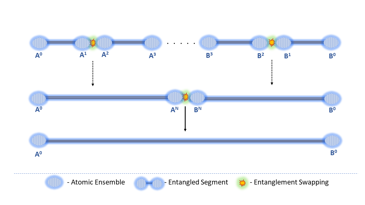
Figure 1: (color online) Working of quantum repeaters. To generate entanglement between two distant nodes $A^{0}$ and $B^{0}$, we start by dividing the total distance into smaller segments $A^{0}-A^{1}$,$A^{2}-A^{3}$,…,$B^{3}-B^{2}$,$B^{1}-B^{0}$ with their corresponding nodes. Entanglement is first generated in the smaller segments between each of these nodes independently. By entanglement swapping between two neighbouring nodes, e.g. $A^{1}$ and $A^{2}$, the entanglement can be extended over a longer segment $A^{0}-A^{3}$. With every successful entanglement swapping step, the generated extended entanglement between two nodes on a segment must be purified. By successive swapping and purification in a hierarchical manner, entanglement can be generated over the original distance between $A^{0}$-$B^{0}$.

Then, entanglement can be generated between two adjacent segments by entanglement swapping using neighboring systems (Bennett et al. (1993),Zukowski et al. (1993)). This process can be repeated until entanglement is generated over the full length. At each step though, the entanglement needs to be purified which is a probabilistic process. Thus, to extend entanglement over two adjacent segments one has to wait till entanglement is generated and purified over each segment Duan et al. (2001). The upshot is that quantum repeater protocols require quantum memories (Duan et al. (2001),Sangouard et al. (2011)) that can store the entanglement for one segment till it is created in the neighboring segment.

In 2001, the DLCZ quantum repeater scheme was introduced. This scheme showed a way to generate heralded entanglement over a distance by using atomic ensembles as individual memory units in combination with linear optics and single-photon detectors. The atomic ensembles form the physical systems or nodes at the end of each segment which can store de-localized spin-wave state when entangled. These nodes are connected by fiber optic cables which serve as the communication channels between ensembles allowing efficient transfer of photons. Entanglement between two neighbouring nodes on adjacent segments can be generated by converting the stored spin-waves in the atomic ensembles into correlated photons and performing beam-splitter measurements on them. The generation and detection of a single photon from the atomic ensemble, in the absence of which way information, makes the two segments get entangled. Memory nodes based on atomic ensembles as opposed to single atoms make strong coupling between atoms and photons possible due to collective effects of a large number of atoms. A brief description of the DLCZ scheme and the collective effects in atomic ensembles is provided in Sec. II for completeness. Following the DLCZ scheme, many experiments have demonstrated remarkable advances towards quantum repeaters (Pu et al. (2017),Chou et al. (2005),Chou et al. (2007)).

The atomic ensembles that act as individual nodes to store de-localized quantum entangled states must satisfy a few important properties. They should have long storage lifetimes and high retrieval efficiency Sangouard et al. (2011). Storage lifetimes of about milliseconds to seconds have been achieved in quantum memories with atomic gases (Zhao et al. (2009a),Zhao et al. (2009b),Yang et al. (2016),Dudin et al. (2013)). Intrinsic retrieval efficiency (IRE) is defined as the probability of retrieving an idler photon in a particular spatio-temporal mode from the stored spin-wave excitation in the atomic ensemble conditioned on the successful detection of signal photon in the write process. Detailed theoretical description of IRE is given in Sec. III. The spatio-temporal mode of the signal and the idler photon must have a high overlap with single mode optical fibers which are used in experiments to collect and propagate these photons for interference and detection. In our definition of the intrinsic retrieval efficiency, we include contributions from mode-overlap between emitted photon field and the optical fiber field as it is an integrated part of photon read out process in experiments. Because of the collective effects of atoms involved in the light-matter interaction, the read-out photon is highly correlated with the spin-wave excitation stored in the atomic ensemble. High IRE values are extremely important for reasonable entanglement distribution rates (Duan et al. (2001); Sangouard et al. (2011)). For example, as is stated in Sangouard et al. (2011), 1% reduction in IRE, from 90% to 89%, increases the entanglement distribution time over a distance of 600Km by 10%-14% for the DLCZ protocol and its variants. Calculations in Duan et al. (2001) show that the scaling of the total time of entanglement generation between two distant atomic ensembles with the number of repeater nodes critically depends on the IRE. Free space IRE in experiments with cold atom ensembles is at best about 50% Laurat et al. (2006). For atomic ensembles confined to cavities, IRE of more than 70% has been achieved (Yang et al. (2016),Simon et al. (2007)). The IRE is sensitive to decoherence due to stray magnetic fields, atom loss as well as dephasing of the spin-wave caused by atomic motion. To understand the exact nature of the IRE, it is important to study the full three dimensional profile of the spin-wave excitation stored in the atomic ensemble and how it gets mapped into the transverse (angular) profile of the emitted photon following the read-out process. Our goal in this paper is to understand the intrinsic memory retrieval efficiency by performing a thorough three-dimensional quantum mechanical calculation that also takes into account the mode matching between the emitted photons and single photon collection fibers.

We would like to note that previous efforts to theoretically describe the read-write process using the Maxwell-Bloch formalism work with one dimensional description of the atomic density and electric field propagation Gorshkov et al. (2007). Such a description works well only when we assume that the write beam waist is much broader than the beam waist of the emitted photon. Recent experiments Pu et al. (2017) use beam parameters which are marginally close to not being described by this theoretical treatment. The transverse mode profile of the electric fields play an important role for understanding IRE. As we shall show in our results, IRE is sensitive to the ratio of the beam waists between the write and signal/idler photon beams. It is also important to note that the Maxwell-Bloch approach doesn’t describe the electric field that gets scattered from the atoms. This scattered field is what we are interested in when calculating IRE as the desired spatio-temporal mode of the emitted photon continuously changes to the other scattered modes which contribute to noise. One of the ways of improving the IRE is by increasing the optical depth. This can be achieved by taking longer atomic samples in the direction of light propagation without increasing the overall atomic density. For longer geometries of atomic samples it becomes essential to look at the variation of the transverse profile of the light beams due to diffraction.

A three-dimensional formalism for calculating the field modes of light scattered from an ensemble of hot atomic gas was presented L.M.Duan et al. (2002). In this calculation, the atomic positions were averaged over the duration of interaction with light to get the emitted photon mode profile. This averaging significantly simplifies the calculations to get the mode profile of the photon correlated with the symmetric collective spin wave state. Since, we are interested in describing cold atomic ensembles, such averaging over positions cannot be done. One of the interesting results from this calculation in L.M.Duan et al. (2002) suggested that atomic density fluctuations give rise to intrinsic mode mismatching errors. We find that atomic density fluctuations have a significant role to play when determining IRE.

This paper is organized as follows: in Sec. II the interaction scheme between the atomic ensemble and light is discussed with the aim of understanding the IRE of a quantum memory unit based on such an interaction. In Sec. III a detailed theoretical analysis for the write and read process defining the storage and retrieval of quantum spin wave is presented. Sec. IV focuses on the results obtained by numerical simulations of atoms in a node subject to motion. In the final Sec. V we revisit the results and conclude the discussion.

II Read and write process of an atomic quantum memory

In this section, we will take a close look at the DLCZ scheme and define the associated atoms-light interaction configuration.

As shown in Fig. (1), to generate entanglement over $A^{0}$ and $B^{0}$, we split the intermediate distance into multiple smaller segments and perform entanglement generation for each segment followed by entanglement swapping between neighbouring segments sequentially. Let us look at the entanglement generation step first. A pictorial representation of the setup for entanglement generation between two atomic ensembles on a segment is shown in Fig. (2). The two ensembles $A^{N}$ and $A^{N+1}$ are simultaneously excited with weak Raman pulses (write pulse), such that there is a small but definite probability of one of the ensembles emitting a photon correlated with the coherent spin-wave mode in the atomic ensemble Duan et al. (2001). The photon generated from either of the samples is coupled to optical fibers and made to interfere at a 50-50 beam-splitter coupled to single photon detectors at the output arms. If either of the detectors clicks, that heralds entanglement between the two ensembles. This is how entanglement is generated within each segment of the quantum repeater scheme.

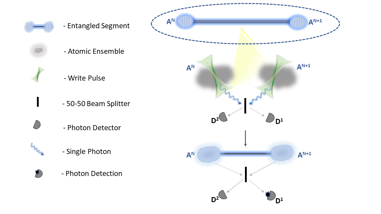
Figure 2: (color online). Entanglement generation between two atomic ensembles $A^{N}$ and $A^{N+1}$. The atomic ensembles to be entangled are simultaneously excited with weak off-resonant Raman pulses, called the write pulse. A photon corresponding to the atomic spin wave mode emitted from any one of the ensembles is sent through the 50-50 beam-splitter. The output arms of the beam-splitter are in-turn coupled to single photon detectors. For ideal photon detectors, a click in any of the two detectors, e.g. $D^{1}$ in this case, heralds the generation of entanglement between the two atomic ensembles $A^{N}$ and $A^{N+1}$.

Once we have two such adjacent entangled segments eg. $A^{0}-A^{N}$ and $B^{N}-B^{0}$ in Fig. (3), we can carry out the next step of entanglement swapping as follows. The ensembles $A^{N}$ and $B^{N}$ are simultaneously excited with strong read-out pulses, such that there is a high probability of a stored spin-wave atomic excitation getting converted into a highly directional photon. These photons are collected and made to interfere at another 50-50 beam-splitter connected also to single photon detectors. If there is a click in either of the detector arms, that would lead to entanglement of the ensembles $A^{0}-B^{0}$. The necessary requirement as discussed previously is that the entanglement in either segment needs to be stored until entanglement in the other segment can be generated and purified. The process of entanglement generation, purification and swapping can now be repeated to create entanglement sequentially between ensembles farther and farther apart. The details of read and write process for each atomic ensemble are given below.

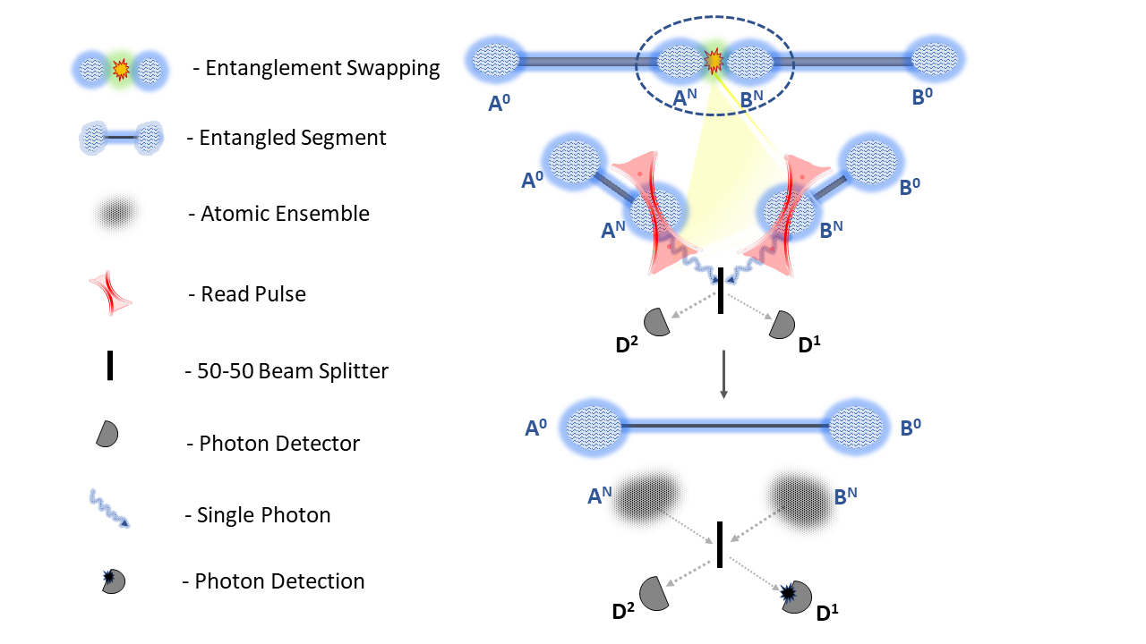
Figure 3: (color online).Entanglement Swapping between two neighbouring entangled segments. Given two entangled segments $A^{0}-A^{N}$ and $B^{N}-B^{0}$, entanglement is generated between atomic ensembles $A^{0}-B^{0}$ by entanglement swapping between ensemble $A^{N}-B^{N}$. The atomic spin-wave modes in the neighbouring ensembles $A^{N}$ and $B^{N}$ are converted into photons using a strong and broad read-out pulse. Photons emitted by the atomic ensembles are coupled to a 50-50 beam-splitter. The output from the beam-splitter is coupled to single photon detectors. Whenever one of the detectors registers a photon, the atomic ensembles $A^{0}-B^{0}$ get entangled due to entanglement swapping.

Consider an atomic ensemble with $N_{a}$ atoms with a $\Lambda$ level structure as shown in Fig. (4). There are two metastable ground levels, $|g\rangle$ and $|s\rangle$ having long lifetimes and an excited level $|e\rangle$. All atoms are initially prepared in the ground state $|g\rangle$. The atoms in the ensemble are acted upon with a weak off-resonant laser pulse, the write-beam, on the $|e\rangle$-$|g\rangle$ transition. With some small probability a single photon, called the signal photon, corresponding to $|e\rangle$-$|s\rangle$ transition gets emitted spontaneously.

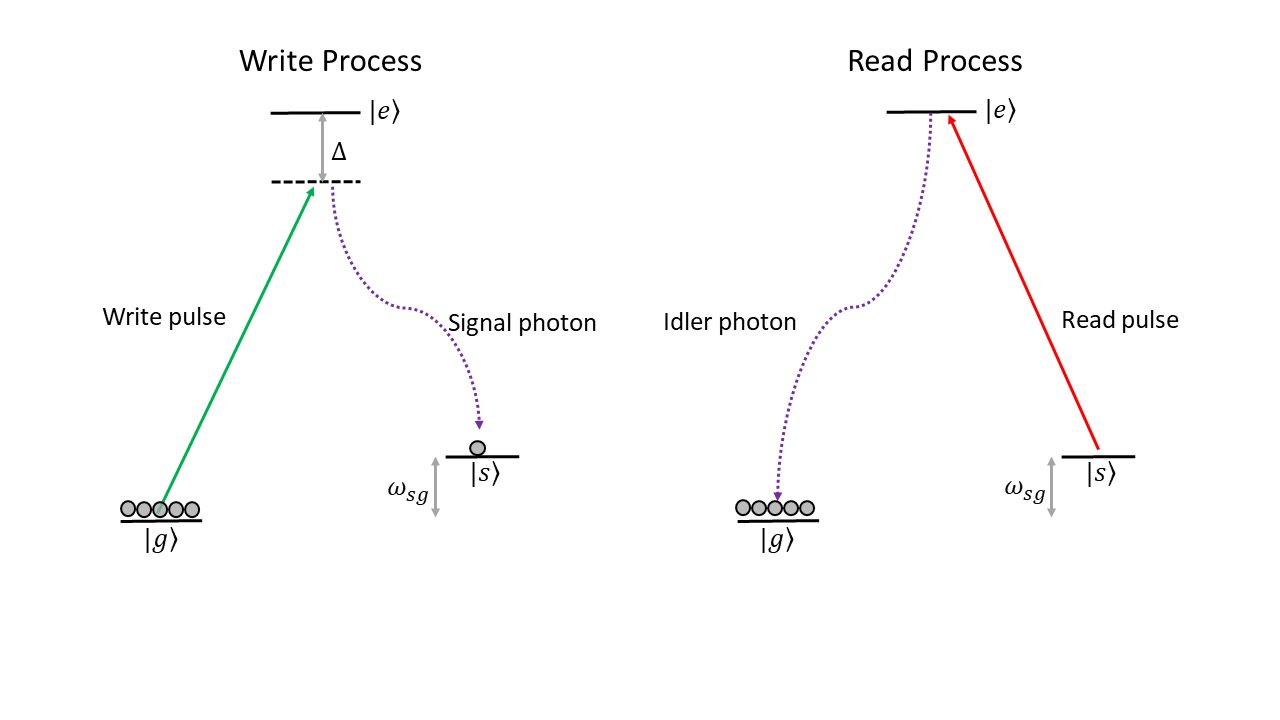
Figure 4: (color online). Atomic level diagram for the DLCZ protocol. Every atom in the atomic ensemble is considered to have a three level $\Lambda$ structure. Levels $|g\rangle$ and $|s\rangle$ are two metastable states separated by frequency equal to $\omega_{sg}$, with forbidden dipole transition between them. Level $|e\rangle$ is an excited state. At $t=0$ all atoms are in the ground state $|g\rangle$. In the write process, the atomic ensemble is excited with a classical write-pulse that is detuned from the $|g\rangle$-$|e\rangle$ transition by a frequency $\Delta$. With the emission and detection of a signal photon on the $|e\rangle$-$|s\rangle$ transition the write process is complete with one atom excited to the $|s\rangle$ level. In the read process, the ensemble is excited with a strong on resonance read-pulse for $|s\rangle$-$|e\rangle$ transition. The emission and detection of a highly directed idler photon from $|e\rangle$-$|g\rangle$ concludes the read process.

This is the two-photon Raman scattering process that results in a transition of one atom from $|g\rangle$ to $|s\rangle$ level. Information of which atom in the ensemble emitted the photon is lost for a far field detection of the photon. This leads to the creation of a coherent collective atomic spin-wave state of the form:

$$|\Psi_{a}\rangle=\sum_{j=1}^{N_{a}}C_{j}e^{\textit{i}(\textbf{k}_{W}-\textbf{k}_{S})\cdot\textbf{r}_{j}}|g\rangle_{1}|g\rangle_{2}...|s\rangle_{j}....|g\rangle_{N_{a}}$$ (1)

where $\mathbf{k}_{W}$ and $\mathbf{k}_{S}$ are the wavevectors associated with the write-beam and the emitted signal photon respectively and $\mathbf{r}_{j}$ is the position vector for $j^{th}$ atom. The complex coefficients $C_{j}$ are dependent on the shape of the laser profiles at the $j^{th}$ atomic position. With the detection of the signal photon, write process is complete and information is now stored in the coherent atomic spin-wave.

Now, we move on to describe the read-process. After a certain time $T_{m}$, the storage time, a strong classical laser pulse (read pulse) resonant with the $|e\rangle$-$|s\rangle$ transition is made to shine on the atomic ensemble such that any atom in the $|s\rangle$ state gets excited to the $|e\rangle$ state. The atom in $|e\rangle$ state emits an idler photon to relax back to the $|g\rangle$ state. The atomic quantum state after this process is proportional to:

$$\sum_{j=1}^{N_{a}}D_{j}e^{\textit{i}(\textbf{k}_{W}-\textbf{k}_{S})\cdot\textbf{r}_{j}}e^{\textit{i}(\textbf{k}_{R}-\textbf{k}_{I})\cdot\textbf{r}^{\prime}_{j}}|g\rangle_{1}|g\rangle_{2}...|g\rangle_{N_{a}}$$ (2)

where, $\mathbf{k}_{R}$ and $\mathbf{k}_{I}$ are the wavevectors corresponding to the read beam and the emitted idler photon respectively. The position of the $j^{th}$ atom after the storage time $T_{m}$ is given by $\mathbf{r}^{\prime}_{j}$. Because of finite temperatures of the atomic sample, $\mathbf{r}_{j}$ is generally different from $\mathbf{r}^{\prime}_{j}$. For the calculations henceforth, we assume that the atomic ensemble is a cold-atom sample having a temperature of about 30$\mu K$ obtained by cooling a MOT sample further via Polarization Gradient Cooling technique. The coefficients $D_{j}$ are weights associated with the $j^{th}$ atom that depend on the atomic positions $\mathbf{r}_{j}$ as well as $\mathbf{r}^{\prime}_{j}$ and properties specific to the atom-light interaction like polarization, dipole moment and beam parameters. Eq. (2) tells us that the amplitude of emission for the idler photon in the $\mathbf{k}_{I}$ direction is determined by interference between all the atoms of the ensemble scaled by factors $D_{j}$. Because of constructive interference between all atom contributions, the idler photon is emitted in a well specified direction based on the phase matching condition.

$$(\textbf{k}_{W}-\textbf{k}_{S})\cdot\textbf{r}_{j}+(\textbf{k}_{R}-\textbf{k}_{I})\cdot\textbf{r}^{\prime}_{j}=0$$ (3)

We shall see from the calculations in the next sections, the intrinsic retrieval efficiency is acutely affected by the interference condition. As discussed in Sangouard et al. (2011), complete constructive interference is possible only when the atoms don’t move within the storage time ($\mathbf{k}_{W}+\mathbf{k}_{R}=\mathbf{k}_{S}+\mathbf{k}_{I}$) or when the beams are colinear ($\mathbf{k}_{W}=\mathbf{k}_{S}$, $\mathbf{k}_{R}=\mathbf{k}_{I}$). In experiments with cold atomic gases, both these conditions are seldom implementable. Because of position dependent weights associated with the angular profile of the light and atomic spin-wave and non-zero energy difference between the two ground levels, unit IRE cannot be achieved.

With the basic idea of the protocol and importance of retrieval efficiency in mind, let us now look at the full derivation of the mathematical expression of retrieval efficiency with a complete 3-D analysis.

III Theoretical formulation of the intrinsic retrieval efficiency

We will now formulate the interaction between light and the atomic ensemble which acts as a temporary storage for quantum entanglement. We shall also describe IRE formally and calculate it using the quantum theory of light-matter interactions. As is already seen in Sec. I, the intrinsic retrieval efficiency is defined as the probability of getting the desired photon from the stored atomic spin-wave.

After interacting with the write beam, the quantum state of the atomic ensemble and the emitted photon is expressed as:

$$|\Psi\rangle_{W}=\int\frac{d^{3}\textbf{k}}{(2\pi)^{3}}\sum_{j=1}^{N_{a}}C_{j}(\textbf{k})|s\rangle_{j}|\textbf{k}\rangle_{ph}$$ (4)

where:

$$|s\rangle_{j}\leftarrow|g\rangle_{1}|g\rangle_{2}...|s\rangle_{j}...|g\rangle_{N_{a}}$$ (5)

and $C_{j}(\mathbf{k})$ is the photon wave function given an atomic excitation for atom $j$ . Sum over $j$ adds contribution of all the atoms of the sample and the integration over $\mathbf{k}$ for all the wave-vectors.

Detection of the write photon can be expressed as the overlap of the above state in Eq. (4) with a transverse Gaussian electric field mode coupled to the single mode optical fiber. The resulting quantum state after this overlap is the obtained spin-wave state. This state after appropriate normalization gives the initial condition of the atomic ensemble for the read process. After the read process, the resulting photon quantum state can be described as:

$$|\Psi\rangle_{R}=\int\frac{d^{3}\textbf{k}}{(2\pi)^{3}}\sum_{j=1}^{N_{a}}D_{j}(\textbf{k})|\textbf{k}\rangle$$ (6)

while the atomic ensemble is back to its ground state $|g\rangle^{\otimes N}=|g\rangle_{1}|g\rangle_{2}...|g\rangle_{N}$. We can again represent detection of the emitted read photon as an overlap of the emitted photon state with transverse Gaussian field. The squared norm of this overlap would correspond to the desired IRE. In the following subsections, we shall derive the explicit expression of this quantity.

III.1 The Write Process

For the atomic level structure given in Fig. (4), in the write process, the atomic ensemble is excited by a weak and short off-resonant Raman pulse (the write pulse) coupled to the $|g\rangle$-$|e\rangle$ transition. We treat this interaction semi-classically, by taking classical light pulse interacting with a quantum atomic system. The electric field associated with the write pulse is given as:

$$\textbf{E}^{w}(\textbf{r},t)=\frac{1}{2}\left[\hat{\epsilon}^{w}E^{w}(\textbf{r},t)e^{\textit{i}(\textbf{k}^{w}\cdot\textbf{r}-\omega^{w}t)}+\text{c.c.}\right]$$ (7)

Where $\omega^{w}=k^{w}c$ is the carrier frequency of the write pulse and $|\mathbf{k}^{w}|=k^{w}$. Also $\hat{\epsilon}^{w}$ is the unit direction of the field. It is assumed to be a square pulse of width $T_{w}$ time units.

The spontaneously emitted photon corresponding to the $|e\rangle$-$|s\rangle$ transition is treated quantum mechanically. The electric field associated with the emitted signal photon is described by the sum of all the free field modes:

$$\hat{\textbf{E}}(\textbf{r})=\sum_{\tau}\int\frac{d^{3}\textbf{k}}{(2\pi)^{3}}\left[\hat{\epsilon}_{\textbf{k},\tau}f(k)e^{\textit{i}\textbf{k}\cdot\textbf{r}}a_{\textbf{k},\tau}+\text{h.c.}\right]$$ (8)

In the above expression, $\mathbf{k}$ stands for the wavevector of the emitted photon and $\tau$ for one of the two independent polarization directions given a wavevector. The operators $a_{\mathbf{k},\tau}$ and its Hermitian conjugate $a^{\dagger}_{\mathbf{k},\tau}$ are the annihilation and creation operators for the given wavevector $\mathbf{k}$ and polarization $\tau$. The dispersion relation is given as $\omega_{k}=|\mathbf{k}|c$. Also for free space normal modes, the expression for the mode function $f(k)$ is:

$$f(k)=\textit{i}\sqrt{\frac{\hbar\omega_{k}}{2\varepsilon_{0}}}$$ (9)

where $\varepsilon_{0}$ is the free space permittivity. Throughout this paper we set $\hbar=1$ for simplicity.

We assume that there is no atom-atom interaction in the system. The atom-field interaction Hamiltonian taken here is the dipole interaction with minimal coupling. Under the rotating wave approximation (RWA) we get the following Hamiltonian given in Eq. (10). Note that spontaneous emission from the state $|e\rangle$ to $|g\rangle$ is ignored as it is not important for our purpose. Taking the energy of the $|g\rangle$ state, $\omega_{g}$, to be our 0 reference, the write Hamiltonian is then:

$$H^{w} = \sum_{\tau}\int\frac{d^{3}\textbf{k}}{(2\pi)^{3}}~{}\omega_{k}a^{\dagger}_{\textbf{k},\tau}a_{\textbf{k},\tau}+\sum_{j=1}^{N_{a}}(\omega_{eg}\sigma_{ee}^{j}+\omega_{sg}\sigma_{ss}^{j})$$ (10)

$$+ \sum_{j=1}^{N_{a}}\bigg{[}\Omega_{eg,j}^{w}e^{\textit{i}(\textbf{k}^{w}\cdot\textbf{r}_{j}-\omega^{w}t)}\sigma_{eg}^{j}$$

$$+ \sum_{\tau}\int\frac{d^{3}\textbf{k}}{(2\pi)^{3}}~{}g_{es,\tau}(\textbf{k})e^{\textit{i}\textbf{k}\cdot\textbf{r}_{j}}\sigma_{es}^{j}a_{\textbf{k},\tau}+\text{h.c.}\bigg{]}$$

where:

$$\omega_{ab} = \omega_{a}-\omega_{b}$$ (11)

$$\sigma^{j}_{\mu\nu} = |\mu\rangle_{j}\langle\nu|$$ (12)

$$\Omega_{eg,j}^{w} = \frac{1}{2}|e|\langle e|\hat{\textbf{r}}|g\rangle\cdot\hat{\epsilon}^{w}E^{w}(\textbf{r}_{j},t)$$ (13)

$$g_{es,\tau}(\textbf{k}) = |e|\langle e|\hat{\textbf{r}}|s\rangle\cdot\hat{\epsilon}_{\textbf{k},\tau}f(k)$$ (14)

We can transform the Hamiltonian into the field interaction picture using the following unitary transformation:

$$U = \exp\Bigg{[}-\textit{i}\sum_{j=1}^{N_{a}}(\omega^{w}\sigma_{ee}^{j}+\omega_{sg}\sigma_{ss}^{j})t$$ (15)

$$-\textit{i}\sum_{\tau}\int\frac{d^{3}\textbf{k}}{(2\pi)^{3}}~{}\omega_{k}a^{\dagger}_{\textbf{k},\tau}a_{\textbf{k},\tau}t\Bigg{]}$$

With this unitary transformation the interaction Hamiltonian is given as:

$$H_{new}=U^{\dagger}H_{old}U+\textit{i}(\partial_{t}U^{\dagger})U$$ (16)

On solving the expression for $H_{new}$ we get:

$$H_{new}^{w} = \sum_{j=1}^{N_{a}}\Delta^{w}\sigma_{ee}^{j}+\sum_{j=1}^{N_{a}}\bigg{[}\Omega_{eg,j}^{w}e^{\textit{i}\textbf{k}^{w}\cdot\textbf{r}_{j}}\sigma_{eg}^{j}$$ (17)

$$+ \sum_{\tau}\int\frac{d^{3}\textbf{k}}{(2\pi)^{3}}~{}g_{es,\tau}(\textbf{k})e^{\textit{i}\textbf{k}\cdot\textbf{r}_{j}-\textit{i}(\omega_{k}-\omega^{w}+\omega_{sg})t}\sigma_{es}^{j}a_{\textbf{k},\tau}$$

$$+ \text{h.c.}\bigg{]}$$

where we have defined $\Delta^{w}=\omega_{eg}-\omega^{w}$ as the detuning of the write pulse from the $|e\rangle$-$|g\rangle$ transition. We can reduce the three level problem to a two level problem by adiabatic elimination of the excited level $|e\rangle$. This approximation is valid if the natural width $\Gamma$ of the excited level and frequency spread of the write pulse around $\omega^{w}$ are significantly smaller compared to the detuning $\Delta^{w}$.

The Hamiltonian after the adiabatic elimination thus obtained after ignoring the Stark shifts in level $|s\rangle$ due to spontaneous emission is given by:

$$H_{new}^{w} = -\sum_{j=1}^{N_{a}}\frac{|\Omega_{eg,j}^{w}|^{2}}{\Delta^{w}}\sigma_{gg}^{j}-\sum_{j=1,\tau}^{N_{a}}\int\frac{d^{3}\textbf{k}}{(2\pi)^{3}}$$ (18)

$$\bigg{[}\frac{\Omega_{eg,j}^{w}g_{es,\tau}^{*}(\textbf{k})}{\Delta^{w}}e^{-\textit{i}(\Delta\textbf{k}\cdot\textbf{r}_{j}-\Delta\omega t)}\sigma_{sg}^{j}a_{\textbf{k},\tau}^{\dagger}$$

$$+\text{h.c.}\bigg{]}$$

where:

$$\Delta\textbf{k} = \textbf{k}-\textbf{k}^{w}$$ (19)

$$\Delta\omega = \omega_{k}-(\omega^{w}-\omega_{sg})$$ (20)

We can perform another unitary transformation, rotating the vector $|g\rangle$ such that the resulting Hamiltonian depends only on the lowering and raising atomic operators. The corresponding unitary transformation is:

$$U=\exp\Bigg{[}\textit{i}\int_{0}^{T_{w}}\sum_{j=1}^{N_{a}}\frac{|\Omega^{w}_{eg,j}|^{2}}{\Delta^{w}}\sigma_{gg}^{j}dt^{\prime}\Bigg{]}$$ (21)

The resulting transformed Hamiltonian is then:

$$H_{new}^{w} = -\sum_{j=1,\tau}^{N_{a}}\int\frac{d^{3}\textbf{k}}{(2\pi)^{3}}\bigg{[}\frac{\Omega_{eg,j}^{w}g_{es,\tau}^{*}(\textbf{k})}{\Delta^{w}}e^{-\textit{i}(\Delta\textbf{k}\cdot\textbf{r}_{j}-\Delta\omega t)}$$ (22)

$$e^{\textit{i}\int_{0}^{T_{w}}\frac{|\Omega^{w}_{eg,j}|^{2}}{\Delta^{w}}dt}\sigma_{sg}^{j}a_{\textbf{k},\tau}^{\dagger}+\text{h.c.}\bigg{]}$$

In the following calculations, we ignore the phase accumulated due to the Stark shift in $|g\rangle$ as it is small in comparison with the other phases accumulated in the duration $T_{w}$.

Let us start with the write Hamiltonian and derive the state of the system under the single photon excitation limit. We consider only single photon excitation as the write laser pulse is weak and off-resonant.

$$H_{new}^{w}=\sum_{j=1,\tau}^{N_{a}}\int\frac{d^{3}\textbf{k}}{(2\pi)^{3}}\big{[}C_{j,\tau}^{w}(\textbf{k},t)\sigma_{gs}^{j}a_{\textbf{k},\tau}+\text{h.c.}\big{]}$$ (23)

We have defined:

$$C_{j,\tau}^{w}(\textbf{k},t) = -\frac{\Omega_{eg,j}^{w*}g_{es,\tau}(\textbf{k})}{\Delta^{w}}e^{\textit{i}(\Delta\textbf{k}\cdot\textbf{r}_{j}-\Delta\omega t)}$$ (24)

We consider the write pulse to be a square pulse with a Gaussian transverse profile travelling in the $+z$ direction whose electric field magnitude is given as:

$$E^{w}(\textbf{r},t)=\textit{Q}^{w}(\textbf{r})V^{w}(t)$$ (25)

With:

$$\textit{Q}^{w}(\textbf{r}) = \frac{E_{0}^{w}}{\sqrt{1+\frac{z^{2}}{z_{w}^{2}}}}e^{-\frac{x^{2}+y^{2}}{W_{w}^{2}\big{(}1+\frac{z^{2}}{z_{w}^{2}}\big{)}}}e^{\textit{i}\big{[}\frac{k^{w}(x^{2}+y^{2})}{2R_{w}(z)}-\psi_{w}(z)\big{]}}$$ (26)

$$V^{w}(t) = \Theta(t)\Theta(T_{w}-t)$$ (27)

Where:

$$z_{w} = \frac{k^{w}W_{w}^{2}}{2}$$ (28)

$$R_{w}(z) = z\left(1+\frac{z_{w}^{2}}{z^{2}}\right)$$ (29)

$$\psi_{w}(z) = \tan^{-1}\frac{z}{z_{w}}$$ (30)

In the above expression, $E_{0}^{w}$ is the peak value of electric field at the center of the Gaussian profile, $W_{w}$ is the beam waist. According to the usual convention of defining Gaussian beam we have, $z_{w}$ as the Rayleigh length, $R_{w}(z)$ as the radius of curvature of the beam wave-front at the position $z$ and $\psi_{w}(z)$ is the associated Gouy phase.

Also in Eq. (25), we have taken the liberty of expressing the electric field magnitude as a product of the spatial part and temporal part since the time taken for the propagation of a single wave-front from one end of the atomic sample to the other end is very small compared to the total time duration of the Gaussian square pulse and $T_{w}\omega^{w}\gg 1$. For a few recent experiments where the widths of the control pulses and the single photon optics is comparable, it becomes necessary to consider the phases introduced due to the transverse profile of these paraxial pulses Pu et al. (2017).

A single photon excited state for the write Hamiltonian defined in Eq. (23) is given as:

$$|\phi\rangle^{w}=\bigg{[}1-\textit{i}\int_{0}^{T_{w}}dt~{}H^{w}(t)\bigg{]}|vac\rangle$$ (31)

where:

$$|vac\rangle=|g\rangle^{\otimes N}|0\rangle_{ph}=|g\rangle_{1}|g\rangle_{2}...|g\rangle_{N}|0\rangle_{ph}$$ (32)

The state $|0\rangle_{ph}$ stands for the absence of any photons in the system.

On substituting the expression for the Hamiltonian, we get:

$$|\phi\rangle^{w} = |vac\rangle+\frac{|e|^{2}\langle e|\textbf{r}|g\rangle\cdot\hat{\epsilon}^{w}}{16\pi^{3}\Delta^{w}}\frac{1}{\sqrt{2\varepsilon_{0}}}\sum_{j=1,\tau}^{N_{a}}Q^{w}(\textbf{r}_{j})$$ (34)

$$\int d^{3}\textbf{k} ~{}\langle s|\textbf{r}|e\rangle\cdot\hat{\epsilon}^{*}_{\textbf{k},\tau}\sqrt{\omega_{k}}e^{\textit{i}(k^{w}\hat{\textbf{z}}-\textbf{k})\cdot\textbf{r}_{j}}$$

$$\int_{0}^{T_{w}}dt ~{}e^{\textit{i}(\omega_{k}-\omega^{w}+\omega_{sg})t}~{}\Theta(T_{w}-t)\Theta(t)|s\rangle_{j}a_{\textbf{k},\tau}^{\dagger}|0\rangle_{ph}$$

$$= |vac\rangle+\frac{|e|^{2}T_{w}\langle e|\textbf{r}|g\rangle\cdot\hat{\epsilon}^{w}}{16\pi^{3}\Delta^{w}}\frac{1}{\sqrt{2\varepsilon_{0}}}\sum_{j=1,\tau}^{N_{a}}Q^{w}(\textbf{r}_{j})$$

$$\int d^{3}\textbf{k} \langle s|\textbf{r}|e\rangle\cdot\hat{\epsilon}^{*}_{\textbf{k}\tau}\sqrt{\omega_{k}}e^{\textit{i}(k^{w}\hat{\textbf{z}}-\textbf{k})\cdot\textbf{r}_{j}}e^{\textit{i}(\omega_{k}-\omega^{w}+\omega_{sg})\frac{T_{w}}{2}}$$

$$\text{sinc}\bigg{[}(\omega_{k}-\omega^{w}+\omega_{sg})\frac{T_{w}}{2}\bigg{]}|s\rangle_{j}a_{\textbf{k},\tau}^{\dagger}|0\rangle_{ph}$$

Under the assumption that the single photon detectors used for the detection of the emitted signal photon are ideal, we can ignore the vacuum component. In the Schrodinger picture, the above expression can then be understood as:

$$|\phi\rangle^{w} = \sum_{\tau}\int d^{3}\textbf{k}~{}\hat{f}^{w}(k,\theta_{k},\phi_{k},\tau)e^{-i\omega_{k}t}a_{\textbf{k},\tau}^{\dagger}|0\rangle_{ph}$$ (35)

where:

$$\hat{f}^{w}(k,\theta_{k},\phi_{k},\tau) = \frac{|e|^{2}T_{w}\langle e|\textbf{r}|g\rangle\cdot\hat{\epsilon}^{w}}{16\pi^{3}\Delta^{w}}\sqrt{\frac{\omega_{k}}{2\varepsilon_{0}}}\sum_{j=1}^{N_{a}}Q^{w}(\textbf{r}_{j})$$

$$\langle s|\textbf{r}|e\rangle\cdot\hat{\epsilon}^{*}_{\textbf{k}\tau}e^{\textit{i}(k^{w}\hat{\textbf{z}}-\textbf{k})\cdot\textbf{r}_{j}}e^{\textit{i}(\omega_{k}-\omega^{w}+\omega_{sg})\frac{T_{w}}{2}}$$

$$\text{sinc}\bigg{[}(\omega_{k}-\omega^{w}+\omega_{sg})\frac{T_{w}}{2}\bigg{]}e^{-i\omega_{sg}t}|s\rangle_{j}$$

In the above equation, we do not consider the phase factors coming from unitary in Eq. (21) as they do not influence the final expression for IRE . We can now trace over the $\omega_{k}$ component because the single photon detector is not sensitive to this value. The trace of $|\phi\rangle^{w}{}^{w}\langle\phi|$ over $\omega_{k}$ diverges for the integration limits going from 0 to $\infty$, but we can restrict the integration from 0 to a finite value of frequency based on the validity of the dipole approximation. For such a situation the dominant contribution comes from a small window around $\omega_{k}=\omega^{w}-\omega_{sg}$. The remaining angular profile of Eq. (LABEL:eq:fhatw) becomes:

$$\hat{f}^{w}(\theta_{k},\phi_{k},\tau) \propto \sum_{j}Q^{w}(\textbf{r}_{j})\langle s|\textbf{r}|e\rangle\cdot\hat{\epsilon}^{*}_{\hat{\textbf{k}},\tau}$$ (37)

$$\times e^{\textit{i}(k^{w}\hat{\textbf{z}}-k^{s}\hat{\textbf{k}})\cdot\textbf{r}_{j}-i\omega_{sg}t}|s\rangle_{j}$$

where $\hat{\textbf{k}}$ is the unit wave-vector and

$$ck^{s} = \omega^{w}-\omega_{sg}$$ (38)

Experimentally, we couple the emitted photon into a single mode optical fiber which in turn couples to the single photon detector. The polarization of the emitted photon is filtered before it is coupled to the optical fiber. The transverse mode associated with the optical fiber is considered to be a Gaussian mode propagating in the $+\hat{z}$ direction. The emitted signal photon mode function will be mostly confined in a small angular region around the direction $+\hat{z}$, overlapping with the paraxial optical fiber mode profile. Thus, we can assume $\hat{\epsilon}^{*}_{\hat{\mathbf{k}},\tau}=\hat{\epsilon}^{*}_{\hat{\mathbf{z}},\tau}$ which can now be taken out of the integration. This approximation is valid since $\hat{\epsilon}^{*}_{\hat{\mathbf{k}},\tau}$ varies slowly over the solid angle around $\hat{\mathbf{z}}$ direction when compared to the rapidly varying phase factor $e^{-\mathit{i}k^{s}\hat{\mathbf{k}}\cdot\mathbf{r}_{j}}$ with changing $\hat{\mathbf{k}}$. Also, the polarization, $\tau$, is fixed by the polarization filters. Thus, we have:

$$\hat{f}^{w}(\theta_{k},\phi_{k}) \propto \sum_{j}Q^{w}(\textbf{r}_{j})e^{\textit{i}(k^{w}\hat{\textbf{z}}-k^{s}\hat{\textbf{k}})\cdot\textbf{r}_{j}}e^{-i\omega_{sg}t}|s\rangle_{j}$$

$$= N_{f}~{}\sum_{j=1}^{N_{a}}Q^{w}(\textbf{r}_{j})e^{\textit{i}(k^{w}\hat{\textbf{z}}-k^{s}\hat{\textbf{k}})\cdot\textbf{r}_{j}}e^{-i\omega_{sg}t}|s\rangle_{j}$$

where $N_{f}$ is the normalization constant for the angular mode function.

The angular mode function of the field associated with the optical fiber can be approximated by a Gaussian mode given below:

$$g^{w}(\theta_{k},\phi_{k}) = N^{w}_{g}~{}e^{-\frac{1}{4}(k^{s}W_{s}\sin\theta_{k})^{2}}$$ (41)

with $N^{w}_{g}$ as the normalization factor.

On taking the overlap between Eq. (LABEL:eq:writefunction) and Eq. (41) in the forward direction we get the spin-wave state $|\phi\rangle^{sw}$ as:

$$|\phi\rangle^{sw} = \int_{0}^{2\pi}d\phi_{k}\int_{0}^{\frac{\pi}{2}}d\theta_{k}\sin\theta_{k}\hat{f}^{w}(\theta_{k},\phi_{k})g^{w*}(\theta_{k},\phi_{k})$$ (43)

$$= N^{sw}\sum_{j=1}^{N_{a}}Q^{w}(\textbf{r}_{j})e^{\textit{i}k^{w}z_{j}}\int_{0}^{\frac{\pi}{2}}d\theta_{k}\sin\theta_{k}e^{-\textit{i}k^{s}z_{j}\cos\theta_{k}}$$

$$J_{0}(k^{s}|\textbf{r}_{j\perp}|\sin\theta_{k})e^{-\frac{1}{4}(k^{s}W_{s}\sin\theta_{k})^{2}}e^{-i\omega_{sg}t}|s\rangle_{j}$$

where $|\mathbf{r}_{j\perp}|=\sqrt{x_{j}^{2}+y_{j}^{2}}$.

For experimental parameters of interest, $k^{s}W_{s}\gg 1$. Thus, only a very small interval of values of $\theta_{k}$ above 0 contributes to the integration, suggesting that we can make the paraxial approximation. Taking the upper limit of integration to $\infty$, $\cos\theta_{k}\approx 1-\theta_{k}^{2}/2$ and $\sin\theta_{k}\approx\theta_{k}$ we get:

$$|\phi\rangle^{sw} = N^{sw}\sum_{j=1}^{N_{a}}Q^{w}(\textbf{r}_{j})e^{\textit{i}(k^{w}-k^{s})z_{j}}\int_{0}^{\infty}d\theta_{k}\theta_{k}$$ (45)

$$J_{0}(k^{s}|\textbf{r}_{j\perp}|\theta_{k})e^{-\theta^{2}_{k}[\frac{1}{4}(W_{s}k^{s})^{2}-\frac{\textit{i}}{2}k^{s}z_{j}]}e^{-i\omega_{sg}t}|s\rangle_{j}$$

$$= N^{sw}\sum_{j=1}^{N_{a}}Q^{w}(\textbf{r}_{j})\frac{e^{\textit{i}(k^{w}-k^{s})z_{j}}}{z_{s}k^{s}\sqrt{1+\frac{z_{j}^{2}}{z_{s}^{2}}}}e^{-\frac{x_{j}^{2}+y_{j}^{2}}{W_{s}^{2}\big{(}1+\frac{z_{j}^{2}}{z_{s}^{2}}\big{)}}}$$

$$e^{-\textit{i}\left[\frac{k^{s}(x_{j}^{2}+y_{j}^{2})}{2R_{s}(z_{j})}-\psi_{s}(z_{j})\right]}e^{-i\omega_{sg}t}|s\rangle_{j}$$

where:

$$z_{s} = \frac{k^{s}W_{s}^{2}}{2}$$ (46)

$$R_{s}(z_{j}) = z_{j}\left(1+\frac{z_{s}^{2}}{z_{j}^{2}}\right)$$ (47)

$$\psi_{s}(z_{j}) = \tan^{-1}\frac{z_{j}}{z_{s}}$$ (48)

The normalization $N^{sw}$ need not be determined as it corresponds to the success rate of the write process and does not affect the desired IRE. We now proceed to the read process, where the spin-wave state is read out and a idler (read) photon is emitted after a memory storage time interval $T_{m}$.

III.2 The Read Process

Let us begin by formulating the read Hamiltonian in a way similar to the write Hamiltonian. In the read process, a short but strong classical laser pulse on resonance with the $|e\rangle$-$|s\rangle$ transition is made to interact with the atomic ensemble. The photon emitted from the $|e\rangle$-$|g\rangle$ transition is collected after polarization filtering. Interaction for the $|s\rangle$-$|e\rangle$ transition is treated semi-classically and the spontaneous photon emission from $|e\rangle$-$|g\rangle$ transition is treated quantum mechanically. Assuming dipolar light-matter interactions and the RWA, we can write the read Hamiltonian as:

$$H^{r} = \sum_{j=1}^{N_{a}}(\omega_{eg}\sigma_{ee}^{j}+\omega_{sg}\sigma_{ss}^{j})+\sum_{\tau}\int\frac{d^{3}\textbf{k}}{(2\pi)^{3}}\omega_{k}a^{\dagger}_{\textbf{k},\tau}a_{\textbf{k},\tau}$$ (49)

$$+ \sum_{j=1}^{N_{a}}\bigg{[}\Omega_{es,j}^{r}e^{\textit{i}(\textbf{k}^{r}\cdot\textbf{r}^{\prime}_{j}-\omega^{r}t)}\sigma_{es}^{j}$$

$$+ \sum_{\tau}\int\frac{d^{3}\textbf{k}}{(2\pi)^{3}}g_{eg,\tau}(\textbf{k})e^{\textbf{i}\textbf{k}\cdot\textbf{r}^{\prime}_{j}}\sigma_{eg}^{j}a_{\textbf{k}\tau}+\text{h.c.}\bigg{]}$$

Definitions of $\Omega_{es,j}^{r}$ and $g_{eg,\tau}$ are analogous to the definitions in Eqs. (13-14). The atomic positions may have changed during $T_{m}$, and are denoted by $\mathbf{r}^{\prime}$.

Using the resonance condition for the $|e\rangle$-$|s\rangle$ transition, the read Hamiltonian in the field interaction picture after the application of the unitary $U$

$$U = \exp\bigg{[}-\textit{i}\sum_{j=1}^{N_{a}}(\omega^{r}\sigma_{ee}^{j}+\omega_{sg}\sigma_{ss}^{j})t$$ (50)

$$-\textit{i}\sum_{\tau}\int\frac{d^{3}\textbf{k}}{(2\pi)^{3}}\omega_{k}a^{\dagger}_{\textbf{k},\tau}a_{\textbf{k},\tau}t\bigg{]}$$

is given as:

$$H^{r}_{new} = \sum_{j=1}^{N_{a}}\omega_{sg}\sigma_{ee}^{j}+\sum_{j=1}^{N_{a}}\bigg{[}\Omega_{es,j}^{r}e^{\textit{i}(\textbf{k}^{r}\cdot\textbf{r}^{\prime}_{j}-\omega_{sg}t)}\sigma_{es}^{j}$$ (51)

$$+ \sum_{\tau}\int\frac{d^{3}\textbf{k}}{(2\pi)^{3}}g_{eg,\tau}(\textbf{k})e^{\textit{i}\textbf{k}\cdot\textbf{r}_{j}-\textit{i}(\omega_{k}-\omega^{r})t}\sigma_{eg}^{j}a_{\textbf{k},\tau}$$

$$+ \text{h.c.}\bigg{]}$$

We consider the classical read-out pulse to be a square pulse propagating in $-z$ direction with a Gaussian transverse profile and its magnitude given as:

$$E^{r}(\textbf{r}) = Q^{r}(\textbf{r})V^{r}(t)$$ (52)

With:

$$Q^{r}(\textbf{r}) = \frac{E_{0}^{r}}{\sqrt{1+\frac{z^{2}}{z_{r}^{2}}}}e^{-\frac{\textbf{r}_{\perp}^{2}}{W_{r}^{2}\big{(}1+\frac{z^{2}}{z_{r}^{2}}\big{)}}}e^{-\textit{i}\big{[}\frac{k^{r}\textbf{r}_{\perp}^{2}}{2R_{r}(z)}-\psi_{r}(z)\big{]}}$$ (53)

$$z_{r} = \frac{k^{r}W_{r}^{2}}{2}$$ (54)

$$R_{r}(z) = z\left(1+\frac{z_{r}^{2}}{z^{2}}\right)$$ (55)

$$\psi_{r}(z) = \tan^{-1}\frac{z}{z_{r}}$$ (56)

$$V^{r}(t) = \Theta(t-T_{p})\Theta(T_{p}+T_{r}-t)$$ (57)

Here, $T_{p}=T_{m}+T_{w}$ is the duration after which the read pulse is sent measured from the beginning of the write pulse and $T_{r}$ is the duration of the read pulse.

Let us consider a general state which satisfies the Schrodinger’s equation as follows:

$$|\phi(t)\rangle^{r} = \sum_{j=1}^{N_{a}}\big{[}A_{j}(t)e^{-i\omega_{sg}t}|s\rangle_{j}|0\rangle_{ph}+B_{j}(t)e^{-i\omega^{r}t}|e\rangle_{j}|0\rangle_{ph}\big{]}$$ (58)

$$+\sum_{\tau}\int\frac{d^{3}\textbf{k}}{(2\pi)^{3}}C_{\tau}(\textbf{k},t)e^{-i\omega_{k}t}|g\rangle^{\otimes N}a^{\dagger}_{\textbf{k},\tau}|0\rangle_{ph}$$

In the above equation, state $|e\rangle_{j}$ is defined similar to state $|s\rangle_{j}$ is Eq. (5). The initial condition for our system is given by Eq. (45).

Applying the Schrodinger’s equation we get:

$$\textit{i}\frac{d|\phi(t)\rangle^{r}}{dt}=H^{r}|\phi(t)\rangle^{r}$$ (59)

$$\textit{i}\dot{A}_{j}(t)=\Omega_{es,j}^{*r}(t)e^{-\textit{i}(\textbf{k}^{r}\cdot\textbf{r}^{\prime}_{j}-\omega_{sg}t)}B_{j}(t)$$ (60)

$$\textit{i}\dot{B}_{j}(t)=\omega_{sg}B_{j}(t)+\Omega_{es,j}^{r}(t)e^{\textit{i}(\textbf{k}^{r}\cdot\textbf{r}^{\prime}_{j}-\omega_{sg}t)}A_{j}(t)$$

$$~{}~{}~{}~{}~{}~{}~{}~{}~{}+\sum_{\tau}\int\frac{d^{3}\textbf{k}}{(2\pi)^{3}}g_{eg,\tau}(\textbf{k})e^{\textit{i}[\textbf{k}\cdot\textbf{r}^{\prime}_{j}-(\omega_{k}-\omega^{r})t]}C_{\tau}(\textbf{k},t)$$

(61)

$$\textit{i}\dot{C}_{\tau}(\textbf{k},t)=\sum_{j}g_{eg,\tau}^{*}(\textbf{k})e^{-\textit{i}[\textbf{k}\cdot\textbf{r}^{\prime}_{j}-(\omega_{k}-\omega^{r})t]}B_{j}(t)$$ (62)

For simplicity, let us assume the dipole moment associated with the Rabi frequency $\Omega_{es,j}^{r}(t)$ to be real. This does not change the final result which only depends on the modulus of this Rabi frequency. Defining:

$$A_{j}(t) = e^{\textit{i}\omega_{sg}t}e^{-\textit{i}\textbf{k}^{r}\cdot\textbf{r}^{\prime}_{j}}e^{\textit{i}\big{[}\frac{k^{r}\textbf{r}_{\perp j}^{2}}{2R_{r}(z_{j})}-\psi_{r}(z_{j})\big{]}}\alpha_{j}(t)$$ (63)

Substitute $A_{j}(t)$ as given above in the rate equations.

$$\textit{i}\dot{\alpha}_{j}(t)=\omega_{sg}\alpha_{j}(t)+\Omega_{es,j}^{r}(t)B_{j}(t)$$ (64)

$$\textit{i}\dot{B}_{j}(t)=\omega_{sg}B_{j}(t)+\Omega_{es,j}^{r}(t)\alpha_{j}(t)$$

$$~{}~{}~{}~{}~{}~{}~{}~{}+\sum_{\tau}\int\frac{d^{3}\textbf{k}}{(2\pi)^{3}}g_{eg,\tau}(\textbf{k})e^{\textit{i}[\textbf{k}\cdot\textbf{r}^{\prime}_{j}-(\omega_{k}-\omega^{r})t]}C_{\tau}(\textbf{k},t)$$

(65)

$$\textit{i}\dot{C}_{\tau}(\textbf{k},t)=\sum_{j}g_{eg,\tau}^{*}(\textbf{k})e^{-\textit{i}[\textbf{k}\cdot\textbf{r}^{\prime}_{j}-(\omega_{k}-\omega^{r})t]}B_{j}(t)$$ (66)

Formally integrating Eq. (66) with $C_{\tau}(\textbf{k},T_{p})=0$ we get:

$$C_{\tau}(\textbf{k},t) = -\textit{i}\sum_{j}\int_{T_{p}}^{t}dt^{\prime}g_{eg,\tau}^{*}(\textbf{k})e^{-\textit{i}[\textbf{k}\cdot\textbf{r}^{\prime}_{j}-(\omega_{k}-\omega^{r})t^{\prime}]}B_{j}(t^{\prime})$$

Substituting the above equation into Eq. (65), we get:

$$\textit{i}\dot{\alpha}_{j}(t) = \omega_{sg}\alpha_{j}(t)+\Omega_{es,j}^{r}(t)B_{j}(t)$$ (68)

$$\textit{i}\dot{B}_{j}(t) = \omega_{sg}B_{j}(t)+\Omega_{es,j}^{r}(t)\alpha_{j}(t)$$

$$- \textit{i}\sum_{l,\tau}\int\frac{d^{3}\textbf{k}}{(2\pi)^{3}}|g_{eg,\tau}(\textbf{k})|^{2}e^{\textit{i}\textbf{k}\cdot(\textbf{r}^{\prime}_{j}-\textbf{r}^{\prime}_{l})}$$

$$\times\int_{T_{p}}^{t}dt^{\prime}e^{-\textit{i}(\omega_{k}-\omega^{r})(t-t^{\prime})}B_{l}(t^{\prime})$$

Substituting:

$$\tilde{B}_{j}(t) = B_{j}(t)e^{\textit{i}\omega_{sg}t}$$ (70)

$$\tilde{\alpha}_{j}(t) = \alpha_{j}(t)e^{\textit{i}\omega_{sg}t}$$ (71)

We get:

$$\dot{\tilde{\alpha}} = -\textit{i}\Omega_{es,j}^{r}(t)\tilde{B}_{j}(t)$$ (72)

$$\dot{\tilde{B}}_{j}(t) = -\textit{i}\Omega_{es,j}^{r}(t)\tilde{\alpha}_{j}(t)-\int_{T_{p}}^{t}dt^{\prime}I_{j}(t,t^{\prime})$$ (73)

where:

$$I_{j}(t,t^{\prime})=I^{(1)}_{j}(t,t^{\prime})+I^{(2)}_{j}(t,t^{\prime})$$ (74)

with:

$$I^{(1)}_{j}(t,t^{\prime}) = \sum_{\tau}\int\frac{d^{3}\textbf{k}}{(2\pi)^{3}}|g_{eg,\tau}(\textbf{k})|^{2}$$ (75)

$$e^{-\textit{i}(\omega_{k}-\omega^{r}-\omega_{sg})(t-t^{\prime})}\tilde{B}_{j}(t^{\prime})$$

$$I^{(2)}_{j}(t,t^{\prime}) = \sum_{\tau}\sum_{l=1,l\neq j}^{N_{a}}\int\frac{d^{3}\textbf{k}}{(2\pi)^{3}}|g_{eg,\tau}(\textbf{k})|^{2}e^{\textit{i}\textbf{k}\cdot(\textbf{r}^{\prime}_{j}-\textbf{r}^{\prime}_{l})}$$

$$e^{-\textit{i}(\omega_{k}-\omega^{r}-\omega_{sg})(t-t^{\prime})}\tilde{B}_{l}(t^{\prime})$$

$$= \sum_{\tau}\sum_{l=1,l\neq j}^{N_{a}}\int\frac{d^{3}\textbf{k}}{(2\pi)^{3}}\frac{\omega_{k}}{2\varepsilon_{0}}|\textbf{d}_{eg}\cdot\hat{\epsilon}_{\textbf{k},\tau}|^{2}e^{\textit{i}\textbf{k}\cdot(\textbf{r}^{\prime}_{j}-\textbf{r}^{\prime}_{l})}$$

$$e^{-\textit{i}(\omega_{k}-\omega^{r}-\omega_{sg})(t-t^{\prime})}\tilde{B}_{l}(t^{\prime})$$

$$= \sum_{l=1,l\neq j}^{N_{a}}\int\frac{d^{3}\textbf{k}}{(2\pi)^{3}}\frac{\omega_{k}}{2\varepsilon_{0}}\textbf{d}_{eg}\cdot[I-\hat{\textbf{k}}\hat{\textbf{k}}]\cdot\textbf{d}_{eg}^{*}$$

$$e^{\textit{i}\textbf{k}\cdot(\textbf{r}^{\prime}_{j}-\textbf{r}^{\prime}_{l})}e^{-\textit{i}(\omega_{k}-\omega^{r}-\omega_{sg})(t-t^{\prime})}\tilde{B}_{l}(t^{\prime})$$

$$= \sum_{l=1,l\neq j}^{N_{a}}\int_{0}^{\infty}\frac{dkk^{3}c}{16\pi^{3}\varepsilon_{0}}\int d\Omega_{k}\textbf{d}_{eg}\cdot[I-\hat{\textbf{k}}\hat{\textbf{k}}]\cdot\textbf{d}_{eg}^{*}$$

$$e^{\textit{i}\textbf{k}\cdot(\textbf{r}^{\prime}_{j}-\textbf{r}^{\prime}_{l})}e^{-\textit{i}(kc-\omega^{r}-\omega_{sg})(t-t^{\prime})}\tilde{B}_{l}(t^{\prime})$$

$$= \sum_{l=1,l\neq j}^{N_{a}}\int_{0}^{\infty}\frac{dkk^{3}c}{4\pi^{2}\varepsilon_{0}}e^{-\textit{i}(kc-\omega^{r}-\omega_{sg})(t-t^{\prime})}\tilde{B}_{l}(t^{\prime})$$

$$\bigg{\{}\textbf{d}_{eg}\cdot\bigg{[}I-\frac{\textbf{r}_{jl}\textbf{r}_{jl}}{|\textbf{r}_{jl}|^{2}}\bigg{]}\cdot\textbf{d}_{eg}^{*}~{}j_{0}(k|\textbf{r}_{jl}|)$$

$$-\textbf{d}_{eg}\cdot\bigg{[}I-3\frac{\textbf{r}_{jl}\textbf{r}_{jl}}{|\textbf{r}_{jl}|^{2}}\bigg{]}\cdot\textbf{d}_{eg}^{*}\frac{j_{1}(k|\textbf{r}_{jl}|)}{k|\textbf{r}_{jl}|}\bigg{\}}$$

Where we have defined:

$$\textbf{r}_{jl} = \textbf{r}^{\prime}_{j}-\textbf{r}^{\prime}_{l}$$ (81)

In the above equation, $j_{0}(x)$ and $j_{1}(x)$ are spherical Bessel functions of the first kind. Terms with $j\neq l$ in Eq. (III.2) denote atom-atom interactions induced by the quantized electric field which correspond to re-absorption of the emitted photon field. For experimental atomic densities of interest, the average number of atoms separated by a distance of about a $\lambda=2\pi c/\omega^{r}$ is less than 1. For such low densities we can ignore the re-absorption terms from our calculations, keeping only the terms where $j=l$ in Eq. (74). Then:

$$I_{j}(t,t^{\prime}) = I_{j}^{(1)}(t,t^{\prime})$$

$$= \int_{0}^{\infty}d\omega\frac{\omega^{3}}{6\pi^{2}\varepsilon_{0}c^{3}}|\textbf{d}_{eg}|^{2}e^{-\textit{i}(\omega-\omega^{r}-\omega_{sg})(t-t^{\prime})}\tilde{B}_{j}(t^{\prime})$$

$$= \frac{(\omega^{r}+\omega_{sg})^{3}|\textbf{d}_{eg}|^{2}}{6\pi^{2}\varepsilon_{0}c^{3}}2\pi\delta(t-t^{\prime})\tilde{B}_{j}(t^{\prime})$$ (84)

$$\equiv \Gamma_{eg}\delta(t-t^{\prime})\tilde{B}_{j}(t^{\prime})$$ (85)

where we use the Wigner-Weisskopf approximation Berman and Malinovsky (2010). $\Gamma_{eg}$ is the rate of spontaneous emission from $|e\rangle$ to $|g\rangle$. Substituting Eq. (85) into Eq. (73) we get

$$\dot{\tilde{\alpha}}(t) = -\textit{i}\Omega_{es,j}^{r}(t)\tilde{B}_{j}(t)$$ (86)

$$\dot{\tilde{B}}_{j}(t) = -\textit{i}\Omega_{es,j}^{r}(t)\tilde{\alpha}_{j}(t)-\gamma_{eg}\tilde{B}_{j}(t)$$ (87)

where $\gamma_{eg}=\Gamma_{eg}/2$.

For the electric field given in Eq. (52), $\Omega_{es,j}^{r}$ is non-zero only when $T_{p}\leq t\leq T_{p}+T_{r}$. For $t>T_{p}+T_{r}$:

$$\dot{\tilde{\alpha}}(t) = 0$$ (88)

$$\dot{\tilde{B}}_{j}(t) = -\gamma_{eg}\tilde{B}_{j}(t)$$ (89)

Thus, for $t>T_{p}+T_{r}$

$$\tilde{\alpha}(t) = \tilde{\alpha}(T_{p}+T_{r})$$ (90)

$$\tilde{B}_{j}(t) = \tilde{B}_{j}(T_{p}+T_{r})~{}e^{-\gamma_{eg}(t-T_{p}-T_{r})}$$ (91)

Now let us evaluate the solution to the rate equations (Eqs. 86-87) for $T_{p}\leq t\leq T_{p}+T_{r}$. This set of two first order differential equations can be combined into a single second order differential equation given as:

$$\ddot{\tilde{B}}_{j}(t) = -(\Omega_{es,j}^{r})^{2}\tilde{B}_{j}(t)-\gamma_{eg}\dot{\tilde{B}}_{j}(t)$$ (92)

Let $\tilde{\Omega}_{es,j}\equiv\sqrt{(\Omega^{r}_{es,j})^{2}-\frac{\gamma_{eg}^{2}}{4}}$. The solution to the Eq. (92) is:

$$\tilde{B}_{j}(t)=C_{1}e^{(-\frac{\gamma_{eg}}{2}-\textit{i}\tilde{\Omega}_{es,j})t}+C_{2}e^{(-\frac{\gamma_{eg}}{2}+\textit{i}\tilde{\Omega}_{es,j})t}$$ (93)

Using the initial conditions at $t=T_{p}$ we get:

$$C_{1} = \frac{\Omega_{es,j}^{r}}{2\tilde{\Omega}_{es,j}}\alpha_{j}(T_{P})e^{(\frac{\gamma_{eg}}{2}+\textit{i}\tilde{\Omega}_{es,j}+\textit{i}\omega_{sg})T_{p}}$$ (94)

$$C_{2} = -\frac{\Omega_{es,j}^{r}}{2\tilde{\Omega}_{es,j}}\alpha_{j}(T_{P})e^{(\frac{\gamma_{eg}}{2}-\textit{i}\tilde{\Omega}_{es,j}+\textit{i}\omega_{sg})T_{p}}$$ (95)

Evaluating $C_{\textbf{k},\tau}(t)$ (Eq. LABEL:eq:c-coeff) using Eq. (70) and Eqs. (94-95) with the definition $\Delta_{k}^{r}\equiv(\omega_{k}-\omega^{r}-\omega_{sg})$ we get:

$$C_{\tau}(\textbf{k},t) = -\sum_{j}g_{eg,\tau}^{*}(\textbf{k})\frac{\Omega_{es,j}^{r}}{\tilde{\Omega}_{es,j}}\alpha_{j}(T_{p})e^{(\frac{\gamma_{eg}}{2}+\textit{i}\omega_{sg})T_{p}}e^{-\textit{i}\textbf{k}\cdot\textbf{r}^{\prime}_{j}}\int_{T_{p}}^{t}dt^{\prime}e^{\textit{i}(\omega_{k}-\omega^{r}-\omega_{sg})t^{\prime}-\frac{\gamma_{eg}}{2}t^{\prime}}\sin[\tilde{\Omega}_{es,j}(t^{\prime}-T_{p})]$$

$$= -\sum_{j}g_{eg,\tau}^{*}(\textbf{k})\Omega_{es,j}^{r}\alpha_{j}(T_{p})e^{\textit{i}(\omega_{k}-\omega^{r})T_{p}}e^{-\textit{i}\textbf{k}\cdot\textbf{r}^{\prime}_{j}}$$

$$\times\frac{e^{(-\frac{\gamma_{eg}}{2}+\textit{i}\Delta_{k}^{r})(t-T_{p})}\left\{\cos[\tilde{\Omega}_{es,j}(t-T_{p})]-\frac{\textit{i}\Delta_{k}^{r}-\gamma_{eg}/2}{\tilde{\Omega}_{es,j}}\sin[\tilde{\Omega}_{es,j}(t-T_{p})]\right\}-1}{(\Delta_{k}^{r}-\tilde{\Omega}_{es,j}+\textit{i}\frac{\gamma_{eg}}{2})(\Delta_{k}^{r}+\tilde{\Omega}_{es,j}+\textit{i}\frac{\gamma_{eg}}{2})}$$

At $t=T_{p}+T_{r}$ we get:

$$C_{\tau}(\textbf{k},T_{p}+T_{r}) = -\sum_{j}g_{eg,\tau}^{*}(\textbf{k})\Omega_{es,j}^{r}\alpha_{j}(T_{p})e^{\textit{i}(\omega_{k}-\omega^{r})T_{p}}e^{-\textit{i}\textbf{k}\cdot\textbf{r}^{\prime}_{j}}\frac{e^{(-\frac{\gamma_{eg}}{2}+\textit{i}\Delta_{k}^{r})T_{r}}\left[\cos(\tilde{\Omega}_{es,j}T_{r})-\frac{\textit{i}\Delta_{k}^{r}-\gamma_{eg}/2}{\tilde{\Omega}_{es,j}}\sin(\tilde{\Omega}_{es,j}T_{r})\right]-1}{(\Delta_{k}^{r}-\tilde{\Omega}_{es,j}+\textit{i}\frac{\gamma_{eg}}{2})(\Delta_{k}^{r}+\tilde{\Omega}_{es,j}+\textit{i}\frac{\gamma_{eg}}{2})}$$

We can now find the explicit expression for $C_{\tau}(\textbf{k},t)$ when $t>T_{p}+T_{r}$:

$$C_{\tau}(\textbf{k},t) = C_{\tau}(\textbf{k},T_{p}+T_{r})-\textit{i}\sum_{j}\int_{T_{p}+T_{r}}^{t}dt^{\prime}$$ (98)

$$g_{eg,\tau}^{*}(\textbf{k})e^{-\textit{i}[\textbf{k}\cdot\textbf{r}^{\prime}_{j}-(\omega_{k}-\omega^{r})t^{\prime}]}B_{j}(t^{\prime})$$

$$C_{\tau}(\textbf{k},t) = C_{\tau}(\textbf{k},T_{p}+T_{r})-\sum_{j}g_{eg,\tau}^{*}(\textbf{k})\frac{\Omega_{es,j}^{r}}{\tilde{\Omega}_{es,j}}\alpha_{j}(T_{p})$$

$$e^{-(\frac{\gamma_{eg}}{2}+\textit{i}\omega_{sg})T_{r}}\sin(\tilde{\Omega}_{es,j}T_{r})$$

$$e^{-\textit{i}\textbf{k}\cdot\textbf{r}^{\prime}_{j}}e^{\textit{i}\omega_{sg}(T_{p}+T_{r})}e^{\gamma_{eg}(T_{p}+T_{r})}$$

$$\times\frac{e^{(\textit{i}\Delta_{k}^{r}-\gamma_{eg})t}-e^{(\textit{i}\Delta_{k}^{r}-\gamma_{eg})(T_{p}+T_{r})}}{\textit{i}\Delta_{k}^{r}-\gamma_{eg}}$$

Finally:

$$C_{\tau}(\textbf{k},t) = -\sum_{j}g_{eg,\tau}^{*}(\textbf{k})\Omega_{es,j}^{r}\alpha_{j}(T_{p})e^{-\textit{i}\textbf{k}\cdot\textbf{r}^{\prime}_{j}}$$

$$\Bigg{\{} e^{\textit{i}\Delta_{k}^{r}(T_{p}+T_{r})}e^{\textit{i}\omega_{sg}T_{p}}e^{-\frac{\gamma_{eg}}{2}T_{r}}$$

$$\Bigg{[}\frac{\cos(\tilde{\Omega}_{es,j}T_{r})-\frac{\textit{i}\Delta_{k}^{r}-\gamma_{eg}/2}{\tilde{\Omega}_{es,j}}\sin(\tilde{\Omega}_{es,j}T_{r})}{(\Delta_{k}^{r}-\tilde{\Omega}_{es,j}+\textit{i}\frac{\gamma_{eg}}{2})(\Delta_{k}^{r}+\tilde{\Omega}_{es,j}+\textit{i}\frac{\gamma_{eg}}{2})}$$

$$+\frac{\sin(\tilde{\Omega}_{es,j}T_{r})}{\tilde{\Omega}_{es,j}}\frac{e^{(\textit{i}\Delta_{k}^{r}-\gamma_{eg})(t-T_{p}-T_{r})}-1}{\textit{i}\Delta_{k}^{r}-\gamma_{eg}}\Bigg{]}$$

$$- \frac{e^{\textit{i}(\Delta_{k}^{r}+\omega_{sg})T_{p}}}{(\Delta_{k}^{r}+\textit{i}\frac{\gamma_{eg}}{2}-\tilde{\Omega}_{es,j})(\Delta_{k}^{r}+\textit{i}\frac{\gamma_{eg}}{2}+\tilde{\Omega}_{es,j})}\Bigg{\}}$$

Substituting $\alpha_{j}(T_{p})$ back using Eq. (63) and defining:

$$\phi^{r}(\textbf{r}^{\prime}_{j}) = \frac{k^{r}\textbf{r}_{\perp j}^{{}^{\prime}2}}{2R_{r}(z^{\prime}_{j})}-\psi_{r}(z^{\prime}_{j})$$ (101)

we get:

$$C_{\tau}(\textbf{k},t) = -\sum_{j}g_{eg,\tau}^{*}(\textbf{k})\Omega_{es,j}^{r}A_{j}(T_{p})e^{\textit{i}\textbf{k}^{r}\cdot\textbf{r}^{\prime}_{j}}e^{-\textit{i}\phi^{r}(\textbf{r}^{\prime}_{j})}$$ (102)

$$\times e^{-\textit{i}\textbf{k}\cdot\textbf{r}^{\prime}_{j}}\zeta(\omega_{k},\textbf{r}^{\prime}_{j},t)$$

where:

$$\zeta(\omega_{k},\textbf{r}^{\prime}_{j},t) = e^{\textit{i}\Delta_{k}^{r}(T_{p}+T_{r})}e^{-\frac{\gamma_{eg}}{2}T_{r}}$$ (103)

$$\Bigg{[} \frac{\cos(\tilde{\Omega}_{es,j}T_{r})-\frac{\textit{i}\Delta_{k}^{r}-\frac{\gamma_{eg}}{2}}{\tilde{\Omega}_{es,j}}\sin(\tilde{\Omega}_{es,j}T_{r})}{(\Delta_{k}^{r})^{2}-(\Omega^{r}_{es,j})^{2}+\textit{i}\gamma_{eg}\Delta_{k}^{r}}$$

$$+\frac{\sin(\tilde{\Omega}_{es,j}T_{r})}{\tilde{\Omega}_{es,j}}\frac{e^{(\textit{i}\Delta_{k}^{r}-\gamma_{eg})(t-T_{p}-T_{r})}-1}{\textit{i}\Delta_{k}^{r}-\gamma_{eg}}\Bigg{]}$$

$$- \frac{e^{\textit{i}\Delta_{k}^{r}T_{p}}}{(\Delta_{k}^{r})^{2}-(\Omega^{r}_{es,j})^{2}+\textit{i}\gamma_{eg}\Delta_{k}^{r}}$$

At this point another simplification can be made by taking the experimental conditions into consideration. The read-out pulse generally has a very broad waist size compared to the write pulse i.e. $W_{r}\gg W_{w}$. In this case, we can assume that the Gaussian read-out pulse is spatially broad enough to neglect the dependence of $\Omega_{es,j}^{r}$ on atomic positions. Similarly, we can neglect the phase contributions $\phi^{r}(\mathbf{r}^{\prime}_{j})$. Also, we assume that $\Omega_{es}^{r}>\frac{\gamma_{eg}}{2}$.

The last term of Eq. (103) is the only term that doesn’t have the decay contributions from the excited level. From the experimental perspective, we can choose $\gamma_{eg}T_{r}\gg 1$, thus we can neglect the first two terms:

$$\zeta(\omega_{k},\textbf{r}^{\prime}_{j},t) \approx -\frac{e^{\textit{i}\Delta_{k}^{r}T_{p}}}{(\Delta_{k}^{r})^{2}-(\Omega^{r}_{es})^{2}+\textit{i}\gamma_{eg}\Delta_{k}^{r}}$$ (104)

Incorporating these approximations we have:

$$C_{\tau}(\textbf{k},t) = \Omega_{es}^{r}\sum_{j}g_{eg,\tau}^{*}(\textbf{k})A_{j}(T_{p})e^{\textit{i}\textbf{k}^{r}\cdot\textbf{r}^{\prime}_{j}}e^{-\textit{i}\textbf{k}\cdot\textbf{r}^{\prime}_{j}}$$ (105)

$$\times\frac{e^{\textit{i}\Delta_{k}^{r}T_{p}}}{(\Delta_{k}^{r})^{2}-(\Omega^{r}_{es})^{2}+\textit{i}\gamma_{eg}\Delta_{k}^{r}}$$

After sufficiently long time interval only the $C_{\tau}(\textbf{k},t)$ co-efficient survives. Thus, the final state after the action of the read Hamiltonian can be written as:

$$|\Phi\rangle^{r} = \sum_{\tau}\frac{1}{8\pi^{3}}\int d^{3}\textbf{k}C_{\tau}(\textbf{k},t)e^{-i\omega_{k}t}|g\rangle^{\otimes N}a_{\textbf{k}\tau}^{\dagger}|0\rangle_{ph}$$

We see that the mode function in Eq. (LABEL:eq:readmode) peaks for a small range of values of $\omega_{k}$. We can take the frequency at which the photon gets emitted by setting $\Delta_{k}^{r}\pm\Omega^{r}_{es}=0$. Since $\omega^{r}\gg\Omega^{r}_{es}$, taking $\Delta_{k}^{r}=0$ is a good approximation. Then by tracing over the frequency part we can now write the angular part of the emitted photon as:

$$\hat{f}^{r}(\theta_{k},\phi_{k},\tau) = \sum_{j}g_{eg,\tau}^{*}(\theta_{k},\phi_{k})A_{j}(T_{p})e^{\textit{i}\textbf{k}^{r}\cdot\textbf{r}^{\prime}_{j}}e^{-\textit{i}k^{i}\hat{\textbf{k}}\cdot\textbf{r}^{\prime}_{j}}$$ (107)

$$\frac{\omega^{r}+\omega_{sg}}{\sqrt{8\pi^{2}\gamma_{eg}c^{3}}}|g\rangle^{\otimes N}$$

where:

$$ck^{i} = \omega^{r}+\omega_{sg}$$ (108)

Using arguments similar to those used in the write part we assume $g^{*}_{ge,\tau}(\theta_{k},\phi_{k})$ varies slowly for the relevant values of $\theta_{k},\phi_{k}$ around $\theta_{k}=\pi$. Thus, fixing the wave-vector direction to be $-\hat{\mathbf{z}}$, as was done for the write process, we can find the overlap between the angular profile of the emitted photon and the optical fiber used to collect it. The polarization also gets fixed by the polarization filter before coupling into the optical fiber. We can also ignore the phase factors associated with time evolution as the final IRE expression is independent of it. Note that Eq. (107) has the same normalization as $A_{j}(T_{p})$:

$$\int d\Omega_{k}|\hat{f}^{r}(\theta_{k},\phi_{k})|^{2} = \sum_{j}|A_{j}(T_{p})|^{2}$$ (109)

Here we calculate the normalization factor only for the completeness of the formula. In the numerical simulation it is much easier to directly sample the angular dependence and then normalize the function, because $g_{eg,\tau}$ is taken as constant. See Sec. IV for more details. Let the angular profile of the electric field associated with the optical fiber be given as:

$$g^{r}(\theta_{k},\phi_{k})=N_{g}^{r}e^{-\frac{1}{4}(k^{i}W_{i}\sin\theta_{k})^{2}}$$ (110)

In the calculation of the overlap we again use the paraxial approximation due to the fact that $k^{i}W_{i}\gg 1$. The normalization factor $N_{g}^{R}$ under this approximation is given as $N_{g}^{r}=k^{i}W_{i}/\sqrt{2}$. Taking the overlap of the emitted photon profile with the Gaussian collection mode then gives the final atomic state:

$$|\phi\rangle^{fs} = \int_{0}^{2\pi}d\phi_{k}\int_{\frac{\pi}{2}}^{\pi}d\theta_{k}\sin\theta_{k}\hat{f}^{r}(\theta_{k},\phi_{k})g^{r*}(\theta_{k},\phi_{k})$$

$$= \frac{\omega^{r}+\omega_{sg}}{\sqrt{8\pi^{2}\gamma_{eg}c^{3}}}\frac{W_{i}k^{i}}{\sqrt{2}}\sum_{j=1}^{N_{a}}A_{j}(T_{p})e^{-\textit{i}k^{r}z^{\prime}_{j}}\int_{0}^{\frac{\pi}{2}}d\theta_{k}\sin\theta_{k}$$

$$e^{\textit{i}k^{i}z^{\prime}_{j}\cos\theta_{k}}J_{0}(k^{i}|\textbf{r}^{\prime}_{j\perp}|\sin\theta_{k})e^{-\frac{1}{4}(k^{i}W_{i}\sin\theta_{k})^{2}}|g\rangle^{\otimes N}$$

$$= \frac{(\omega^{r}+\omega_{sg})}{\sqrt{8\pi^{2}\gamma_{eg}c^{3}}}\frac{W_{i}k^{i}}{\sqrt{2}}\sum_{j=1}^{N_{a}}A_{j}(T_{p})e^{-\textit{i}k^{r}z^{\prime}_{j}}\frac{e^{\textit{i}k^{i}z^{\prime}_{j}}}{\sqrt{1+\frac{z_{j}^{{}^{\prime}2}}{z_{i}^{2}}}}$$

$$e^{-\frac{x_{j}^{{}^{\prime}2}+y_{j}^{{}^{\prime}2}}{W_{i}^{2}\big{(}1+\frac{z_{j}^{{}^{\prime}2}}{z_{i}^{2}}\big{)}}}e^{\textit{i}\big{[}\frac{k^{i}(x_{j}^{{}^{\prime}2}+y_{j}^{{}^{\prime}2})}{2R_{i}(z^{\prime}_{j})}-\psi_{i}(z^{\prime}_{j})\big{]}}|g\rangle^{\otimes N}$$

$$|\phi\rangle^{fs} \equiv \sum_{j}\Lambda(\textbf{r}_{j},\textbf{r}^{\prime}_{j})|g\rangle^{\otimes N}$$ (114)

where:

$$z_{i} = \frac{k^{i}W_{i}^{2}}{2}$$ (115)

$$R_{i}(z^{\prime}_{j}) = z^{\prime}_{j}\left(1+\frac{z_{i}^{2}}{z_{j}^{{}^{\prime}2}}\right)$$ (116)

$$\psi_{i}(z^{\prime}_{j}) = \tan^{-1}\frac{z^{\prime}_{j}}{z_{i}}$$ (117)

Any subscript or superscript ‘i’ stands for the idler photon. The IRE, $\eta$, is given by the modulus squared of the above overlap.

$$\eta = \frac{\big{|}\sum_{j}\Lambda(\textbf{r}_{j},\textbf{r}^{\prime}_{j})\big{|}^{2}}{\sum_{j}|A_{j}(T_{p})|^{2}}$$ (118)

For an explicit expression for $\Lambda(\textbf{r}_{j},\textbf{r}^{\prime}_{j})$, we substitute $A_{j}(T_{p})$ from Eq. (45), with its normalization factors neglected:

$$\Lambda(\textbf{r}_{j},\textbf{r}^{\prime}_{j}) = \frac{\omega^{r}+\omega_{sg}}{\sqrt{8\pi^{2}\gamma_{eg}c^{3}}}\frac{W_{i}k^{i}}{\sqrt{2}}e^{-\textit{i}k^{r}z^{\prime}_{j}}\frac{e^{\textit{i}k^{i}z^{\prime}_{j}}}{\sqrt{1+\frac{z_{j}^{{}^{\prime}2}}{z_{i}^{2}}}}\frac{e^{-\textit{i}k^{s}z_{j}}}{\sqrt{1+\frac{z_{j}^{2}}{z_{s}^{2}}}}\frac{e^{\textit{i}k^{w}z_{j}}}{\sqrt{1+\frac{z_{j}^{2}}{z_{w}^{2}}}}e^{-\frac{x_{j}^{2}+y_{j}^{2}}{W_{w}^{2}\big{(}1+\frac{z_{j}^{2}}{z_{w}^{2}}\big{)}}}e^{-\frac{x_{j}^{2}+y_{j}^{2}}{W_{s}^{2}\big{(}1+\frac{z_{j}^{2}}{z_{s}^{2}}\big{)}}}e^{-\frac{x_{j}^{{}^{\prime}2}+y_{j}^{{}^{\prime}2}}{W_{I}^{2}\big{(}1+\frac{z_{j}^{{}^{\prime}2}}{z_{i}^{2}}\big{)}}}$$ (119)

$$e^{\textit{i}\big{[}\frac{k^{w}(x_{j}^{2}+y_{j}^{2})}{2R_{w}(z_{j})}-\psi_{w}(z_{j})\big{]}}e^{-\textit{i}\big{[}\frac{k^{s}(x_{j}^{2}+y_{j}^{2})}{2R_{s}(z_{j})}-\psi_{s}(z_{j})\big{]}}e^{\textit{i}\big{[}\frac{k^{i}(x_{j}^{{}^{\prime}2}+y_{j}^{{}^{\prime}2})}{2R_{i}(z^{\prime}_{j})}-\psi_{i}(z^{\prime}_{j})\big{]}}$$

As seen from Eq. (119), the coefficient of the the ground state is a result of weighted interference effects between all the atoms in the ensemble. The overall effect is equivalent to the overlap of four Gaussian beams with different beam parameters. Incidentally, the phase-matching condition cannot be perfectly satisfied even if atoms are stationary as well as for colinear beams. Substituting the values of $k_{s}$ and $k_{i}$ from Eq. (38) and Eq. (108) respectively into Eq. (119), we see that there is always a non-zero phase contribution along the $z$ axis due to $\omega_{sg}$. More precisely, the coherent atomic spin wave has a wavelength of about $2\pi c/(2\omega_{sg})$ in the $z$ direction. For ${}^{87}\mathrm{Rb}$ the hyperfine splitting $|\omega_{sg}|=2\pi\times 6.8\,$GHz, which means $2\pi c/(2\omega_{sg})\approx$ 22mm. Nevertheless, most experiments never use atomic samples having sizes lager than a few mm, so this effect will be small. The Gaussian transverse structure is another contributor that prevents the IRE from being unity.

Let us now use this framework to look at IRE calculated from a numerical simulation of an atomic sample that mimics the write-read process for realistic experimental setup to gain further insight.

IV Numerical Analysis

To avoid the noise associated with detection of the classical write and read pulses instead of emitted signal and idler photons, a skewed beam configuration of the write and read beams is implemented experimentally as is shown in Fig. (5) (Pu et al. (2017),Sangouard et al. (2011),Zhao et al. (2009b),Yang et al. (2016),Simon et al. (2007)). The write and read laser pulses aligned along the same axis are rotated by a small angle $\Theta$ with respect to the alignment axis of the signal and idler collection ports. This can be easily incorporated into our expression of $\eta$. Assume that the expressions for the write and read pulse electric field in Eq. (26) and Eq. (53) is evaluated in a frame of reference rotated along the x-axis by a skew angle $\Theta$ such that the beams propagate along the $\tilde{z}$-direction of this new frame. The signal and idler photon beams propagate along the z-axis in the original frame of reference. We can express the write and read beams in the un-rotated frame of reference by making the following transformations:

$$\tilde{x} =x$$ (120)

$$\tilde{y} =y\cos\Theta-z\sin\Theta$$ (121)

$$\tilde{z} =y\sin\Theta+z\cos\Theta$$ (122)

Here the coordinates with tilde denote those in the rotated frame expressed in terms of the coordinates in the original frame of reference. With this given transformation, we get:

$$\Lambda(\textbf{r}_{j},\textbf{r}^{\prime}_{j}) = \frac{(\omega^{r}+\omega_{sg})}{\sqrt{8\pi^{2}\gamma_{eg}c^{3}}}\frac{W_{i}k^{i}}{\sqrt{2}}\frac{e^{\textit{i}k^{i}z^{\prime}_{j}}e^{-\textit{i}k^{s}z_{j}}e^{\textit{i}k^{w}(y_{j}\sin\Theta+z_{j}\cos\Theta)}e^{-\textit{i}k^{r}(y^{\prime}_{j}\sin\Theta+z^{\prime}_{j}\cos\Theta)}}{\sqrt{1+\frac{z_{j}^{{}^{\prime}2}}{z_{i}^{2}}}\sqrt{1+\frac{z_{j}^{2}}{z_{s}^{2}}}\sqrt{1+\frac{(y_{j}\sin\Theta+z_{j}\cos\Theta)^{2}}{z_{w}^{2}}}}e^{\textit{i}(\psi_{s}(z_{j})-\psi_{i}(z^{\prime}_{j})-\psi_{w}(y_{j}\sin\Theta+z_{j}\cos\Theta)]}$$ (123)

$$e^{-\frac{x_{j}^{2}+y_{j}^{2}}{W_{w}^{2}\big{(}1+\frac{z_{j}^{2}}{z_{w}^{2}}\big{)}}}e^{-\frac{x_{j}^{2}+y_{j}^{2}}{W_{s}^{2}\big{(}1+\frac{z_{j}^{2}}{z_{s}^{2}}\big{)}}}e^{-\frac{x_{j}^{{}^{\prime}2}+(y^{\prime}_{j}\cos\Theta-z^{\prime}_{j}\sin\Theta)^{2}}{W_{i}^{2}\big{[}1+\frac{(y^{\prime}_{j}\sin\Theta+z^{\prime}_{j}\cos\Theta)^{2}}{z_{i}^{2}}\big{]}}}e^{\textit{i}\big{\{}\frac{k^{w}[x_{j}^{2}+(y_{j}\sin\Theta+z_{j}\cos\Theta)^{2}]}{2R_{w}(y_{j}\sin\Theta+z_{j}\cos\Theta)}-\frac{k^{s}(x_{j}^{2}+y_{j}^{2})}{2R_{s}(z_{j})}+\frac{k^{i}(x_{j}^{{}^{\prime}2}+y_{j}^{{}^{\prime}2})}{2R_{i}(z^{\prime}_{j})}\big{\}}}$$

Throughout the numerical analysis we will assume a Gaussian distribution of atoms inside a MOT. After the atoms have been cooled by using cyclic cooling and optical gradient cooling, the atomic sample has a standard deviation of $0.75\,$mm and the temperature of the atomic sample is about tens of $\mu$K. We get a most probable speed $\sqrt{\frac{2k_{B}T}{M}}$ which is about a few cm/s. For Rb atoms with mass $M=87\,a.u.$ at the temperature of $30\,\mu K$, this value is about $7.5\,$cm/s. For the time duration when the spin wave is stored in the atomic ensemble, atomic motion causes degradation of coherence. We introduce this effect in our calculations by assuming ballistic motion of atoms:

$$\textbf{r}^{\prime}_{j} = \textbf{r}_{j}+\textbf{v}_{j}T_{m}$$ (124)

where $\mathbf{v}_{j}$ are drawn from a Maxwell-Boltzmann distribution of velocities. Since the atomic density is not very high, we can ignore collisions. We have neglected the motion of atoms when the write and read pulses interact with the atomic ensemble, since they are short enough to assume that the atoms are stationary for $T_{p}$ and $T_{r}$. The expression for $\eta$ with the velocities included can be derived by substituting Eq. (124) into Eq. (123).

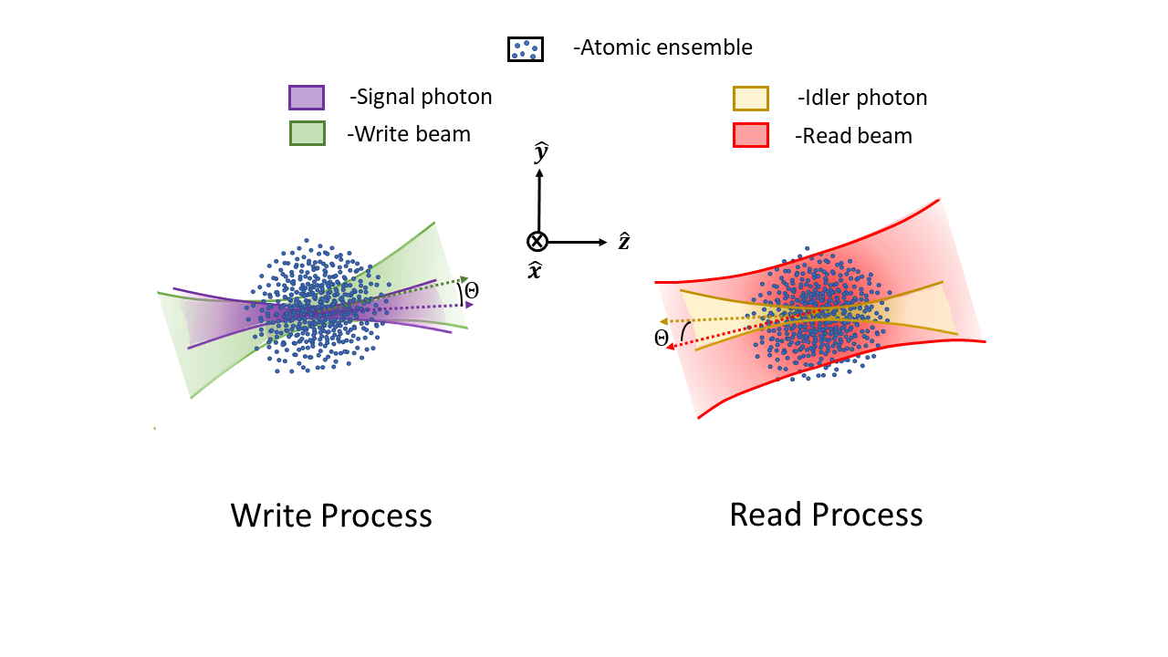
Figure 5: (color online). Configuration of write-read process. Write process: The atomic ensemble is first excited with a classical write pulse, and the emitted signal photon is collected by an optical fiber rotated by an angle $\Theta$ with respect to write pulse axis. The centers of the atomic ensemble and both the beams are aligned. The write beam is generally broader than the signal photon collection beam. Read process: After the write process the ensemble is excited with a very broad read beam which is rotated by an angle $\Theta$ with respect to the idler photon collection beam.

From this equation it becomes clear that the decoherence effect for a non-zero storage time is a direct result of the atomic motion. Let us look at the behaviour of the IRE as a function of the different experimental parameters obtained from a Monte-Carlo sampling of a Gaussian atomic ensemble with spherical symmetry. The range of parameters chosen for all the numerical simulation henceforth have been inspired by experiments reported in Ref. Pu et al. (2017). The atomic samples generated for the numerical simulations have a peak density of the order of $10^{17}$ atoms/$\text{m}^{3}$. An important quantity that captures the strength of interaction between the atomic ensemble and the light is the optical depth of the ensemble. For a given Gaussian density profile the optical depth for a sample of atoms interacting with Gaussian beams is given by the following expression:

$$OD = \frac{2}{\pi}\int^{\infty}_{-\infty}dz\frac{2\pi c_{CG}^{2}\sigma_{0}}{w_{0}^{2}(1+\frac{z^{2}}{z_{w}^{2}})}\int_{0}^{\infty}rdrn_{0}e^{-\frac{r^{2}+z^{2}}{2r_{0}^{2}}}e^{-\frac{2r^{2}}{w_{0}^{2}(1+\frac{z^{2}}{z_{w}^{2}})}}$$

where $w_{0}$ is the Gaussian beam waist at $z=0$, $\sigma_{0}$ the atomic cross-section, $n_{0}$ the peak atomic density and $r_{0}$ as the standard deviation of the atomic distribution. $z_{w}$ is the Rayleigh length for the Gaussian beam given as $k_{0}w_{0}^{2}/2$ for wave-number $k_{0}$. $c_{CG}^{2}$ is the square of the Clebsch-Gordon coefficient associated with the particular atomic transition of interest. We will calculate the optical depth for the interaction with an off-resonant write-pulse corresponding to the 795nm D1 line in ${}^{87}\text{Rb}$. The off-resonant cross-section for this transition is $\sigma_{0}=1.082*10^{-9}\text{cm}^{-2}$ D.A.Steck (2009). For convenience, we set $c_{CG}=1$. The OD can be scaled with the appropriate value of $c_{CG}$ if necessary. For all the numerical results presented in this section, we use $\Delta=2\pi\times\text{10}$MHz and $\omega_{sg}=-2\pi\times\text{6.8}$GHz for $|g\rangle=|5S_{1/2},F=2\rangle$, $|s\rangle=|5S_{1/2},F=1\rangle$ and $|e\rangle=|5P_{1/2},F^{\prime}=2\rangle$ as reported in Pu et al. (2017). The angular wave-function of the idler photon is calculated by sampling the $\theta_{k},\phi_{k}$ dependent part of Eq. (107) (without the $g_{eg,\tau}$ term, which is taken to be a constant according to the argument below Eq. (108)) and is normalized numerically. Then we calculate its overlap with the normalized Gaussian mode of Eq. (110) to get the IRE $\eta$.

First, we will look at the ideal case of stationary atoms, implying a storage time $T_{m}=0$. The IRE thus evaluated is independent of storage time. In Fig. (6), we observe that $\eta$ always remains smaller than unity for the given optical depth OD = 24.7, and different values of skew angle, $\Theta$, as a function of the width ratio (WR) between the write-pulse and the optical fiber mode waists:

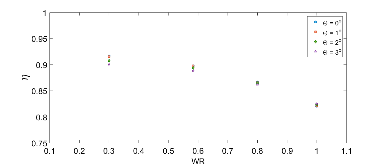
Figure 6: Intrinsic retrieval efficiency $\eta$ as a function of the width ratio WR between the waist width of the signal (idler) optical fiber mode over that of the write beam for different values of skew angle.

$$WR = \frac{W_{i}}{W_{w}}=\frac{W_{s}}{W_{w}}$$ (126)

As we can see, $\eta$ increases with decreasing WR. The reason $\eta$ cannot reach 1 is that there is a mismatch between the photon profile and the optical fiber mode. Fig (7) captures the variation of the IRE as a function of the optical depth of the system for different values of $T_{m}$ with $\Theta=0^{o}$ and WR = 35$\mu$m/60$\mu$m fixed.

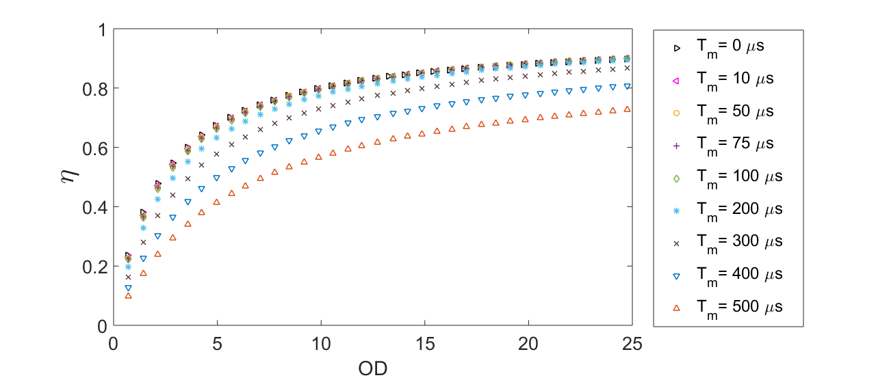
Figure 7: The intrinsic retrieval efficiency as a function of the optical depth for increasing memory storage times $T_{m}$ with skew angle fixed to be 0.

The OD is adjusted by changing the atomic density while keeping the beam parameters constant.

We see the signature of collective enhancement as has been proved in L.M.Duan et al. (2002). The output photon mode that is correlated with the atomic spin wave has higher fractional contribution along the $\theta_{k}=\pi$ direction which increases as the number of atoms goes up. The normalized angular mode $\hat{f}^{r}(\theta_{k},\phi_{k})$ for the idler photon obtained for a dense atomic ensemble is shown in Fig. (8) for $T_{m}=0$ and $\Theta=0^{o}$. This angular profile for an atomic sample with OD = 24.7 and for WR = 35/60 gives about 90% IRE.

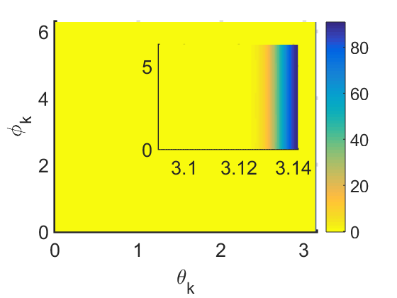
(a) Re[ $f^{r}(\theta_{k},\phi_{k})$]

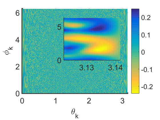
(b) Im[$f^{r}(\theta_{k},\phi_{k})$]

Figure 8: The normalized angular mode function, $f^{r}(\theta_{k},\phi_{k})$, at OD = 24.7, $\Theta=0^{o}$, WR = 35/60 and $\text{T}_{m}=$ $0\,\mu$s.

The real part of the angular mode profile, in the absence of decoherence effects due to non-zero $T_{m}$ and $\Theta$, is plotted in Fig. (8a). It clearly shows a pronounced emission peak near angle $\theta_{k}=\pi$ (shown in the inset) for all azimuthal angles. Apart from the emission around the $\theta_{k}=\pi$ direction, there are noisy contributions present along all other directions as well. The idler photon mode profile has contributions that are prominently from the real part as expected. Without any atomic density fluctuations, that is, replacing the summation over atoms in Eq. (107) with a continuous integration, the imaginary part of the mode function would be identically zero. Thus, imaginary part of the angular profile gives us a scale of fluctuations in all the directions. These fluctuations are related to the density fluctuations of the atomic sample. Important feature to note is that the scale of these fluctuations is very small compared to the scale of the enhanced photon emission to be collected. It is a function of OD and $\Theta$; with decreasing OD and increasing skew angle, we see the relative contributions of the fluctuations in all directions go up.

There is a limit to increasing the optical depth by raising the atomic density because the low atomic density assumption would then breakdown and effects of atom-atom interactions mediated by light will have to be considered Dicke (1954).

Now let us look at the effect of non-zero $T_{m}$ values for skew angle $\Theta=2^{o}$ and WR = 35$\mu$m/60$\mu$m which correspond to the experimental value of parameters from the Tsinghua setup Pu et al. (2017). Fig. (9) shows the variation of the IRE as a function of OD for different values of $T_{m}$ at $\Theta=2^{o}$.

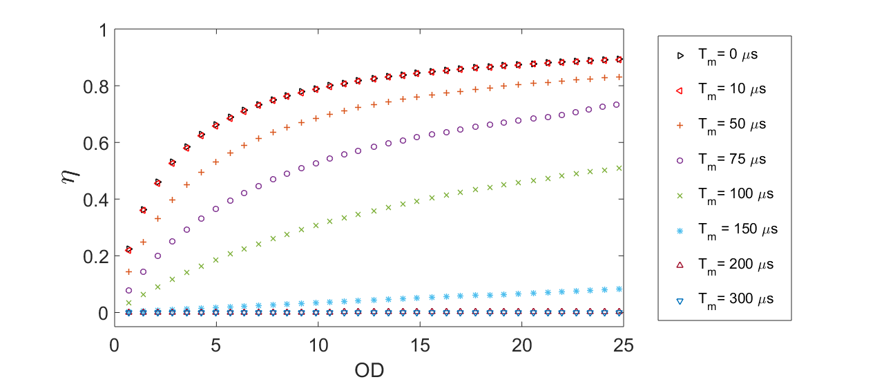
Figure 9: The intrinsic retrieval efficiency as a function of optical depth for increasing storage times $T_{m}$ with skew angle $\Theta=2^{o}$

Comparing Fig. (7) for $\Theta=0^{o}$ and Fig. (9) for $\Theta=2^{o}$, we see the effect of decoherence due to misalignment between the write-read and the signal-idler electric fields. The IRE falls from 80% for $T_{m}=0\,\mu s$ to 50 % for $T_{m}=100\,\mu s$ when skew angle is $2^{o}$ for OD of 24.7 compared to no noticeable change in the $\eta$ value (90%) for $T_{m}$ increasing from $0$ to $100\,\mu s$ when skew angle is set to $0^{o}$. The variation in the IRE for different skew angles and memory storage times at a fixed OD = 24.7 are shown in Fig. (10).

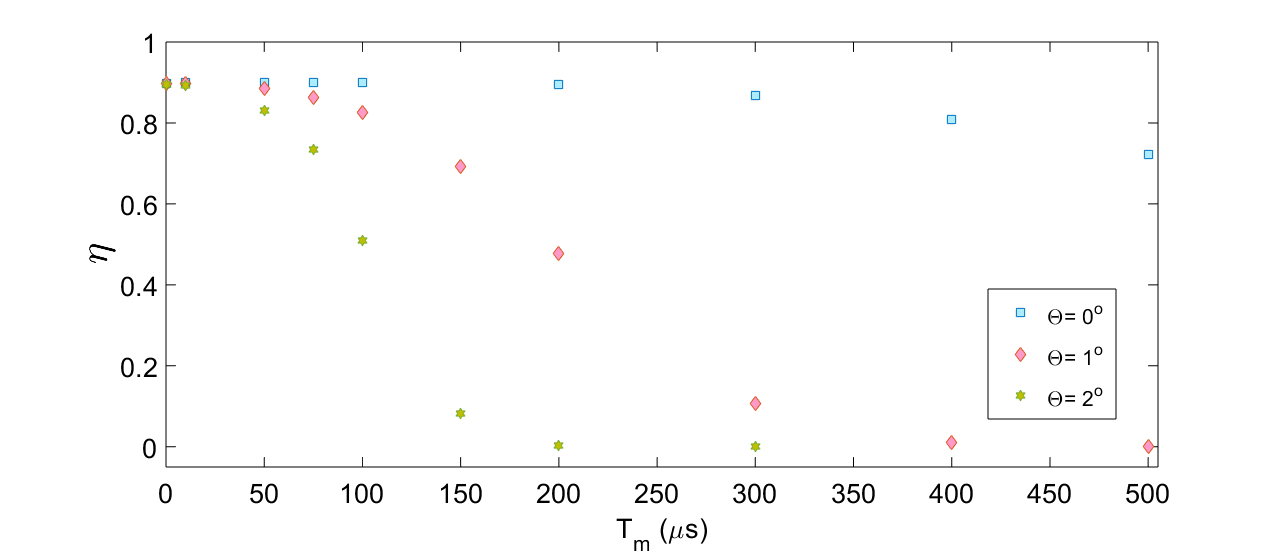
Figure 10: At optical depth = 24.7, intrinsic retrieval efficiency varies as a function of the memory storage time $T_{m}$ for skew angle values $\Theta=(0^{o},1^{o},2^{o})$

We see a rapid decrease in the IRE for non-zero skew angles as the memory storage time is increased. For a retrieval efficiency larger than 80% we can store the atomic spin wave for a maximum of 50 $\mu s$ with $\Theta=2^{o}$ which is not sufficient for implementation of DLCZ quantum repeater protocol efficiently. An important point that must be mentioned here is that the IRE can be increased by using optical traps for the atomic ensemble which restrict the atomic motion and hence help reduce atomic motion induced decoherence, though even after the implementation of such traps, it is still not possible to reach unit retrieval efficiency. Our current theoretical model can be extended to include the effects of optical traps by changing the expression for the atomic positions in Eq. (124) appropriately.

Let us also look at the angular profile for non-zero skew angles and memory storage times. Specifically, we choose a configuration of parameters that gives around $\eta$ = 80%, particularly, $\Theta=1^{o}$ and $T_{m}=100\,\mu s$ [Fig. (11)] and compare it with a value of $\eta$ = 0.3% for $\Theta=2^{o}$ and $T_{m}=200\,\mu s$ [Fig. (12)].

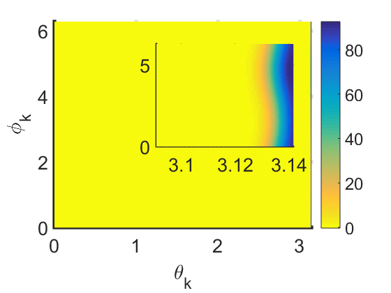
(a) Re[$f^{r}(\theta_{k},\phi_{k})$]

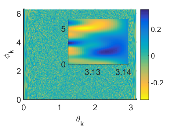
(b) Im[$f^{r}(\theta_{k},\phi_{k})$]

Figure 11: The normalized angular mode function, $f^{r}(\theta_{k},\phi_{k})$, at OD = 24.7, $\Theta=1^{o}$, WR = 35/60 and $T_{m}=100\,\mu s$.

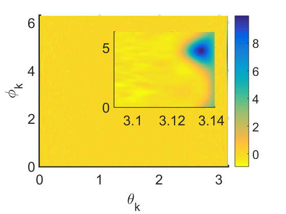
(a) Re[$f^{r}(\theta_{k},\phi_{k})$]

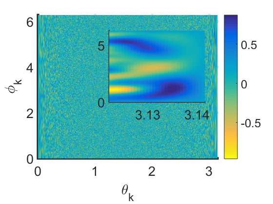
(b) Im[$f^{r}(\theta_{k},\phi_{k})$]

Figure 12: The normalized angular mode function, $f^{r}(\theta_{k},\phi_{k})$, at OD = 24.7, $\Theta=2^{o}$, WR = 35/60 and $T_{m}=200\,\mu s$.

We see that Fig. (11a) shows a prominent contribution around $\theta_{k}=\pi$. On close observation, as shown in the inset, we can detect slight variation in the transverse profile along the $\phi_{k}$ direction for $\theta_{k}\approx\pi$, which becomes more pronounced with larger skew angle and longer storage time in Fig. (12a). The $\theta_{k}$ and $\phi_{k}$ dependence of the observed mode profiles can be attributed to the disruption of symmetry in the z-direction due to non-zero skew angle. As already mentioned, the imaginary part of the mode profile gives an insight about the fluctuations present in all the directions that do not have overlap with the optical fiber electric field. These fluctuations are present in the real part as well, but get washed out by the dominant contribution of the idler photon. Fluctuations in the mode profile are also caused by the atomic density fluctuations in the sample. The fluctuations observed in Fig. (11b) are of the same order as those observed in Fig. (8b). In Fig. (12a) we see higher contribution to the mode profile from all values of $\theta_{k}$ and $\phi_{k}$ when compared to Fig. (8a) and Fig. (11a), and the fluctuations are significantly higher as seen from Fig. (12b). With this we conclude the discussion of the numerical results.

V Discussion

We have formulated a three-dimensional theory to study the intrinsic retrieval efficiency (IRE) during the write-read process for quantum repeater protocols. The focus of this calculation was to describe the quantum mechanical process involved in the interaction of the atomic ensemble with the control light pulses in a three-level $\Lambda$ system. The motivation for this work was primarily to understand the factors that influence the IRE which plays a crucial role in the success of quantum repeater protocols like DLCZ method and its variants Sangouard et al. (2011).

Different interaction strengths involved in the write process and read process were looked at separately. The quantum state obtained by perturbative analysis in the write process provides us with the initial condition for the quantum evolution during the read process. An important result obtained from this calculation is the expression of the IRE as a function of the parameters of the atomic ensemble and control pulses. We show that unit retrieval efficiency is not possible for realistic experimental parameters.

We also show the effects of decoherence introduced due to atomic motion in the sample, which drastically reduce $\eta$ for the skewed configuration of atomic beams. Neglecting the atomic motion for the duration of write and read pulses, within which the accumulated phase is small, only the change in atomic positions during the storage period contributes to the decoherence. In general, for ballistic motion of atoms in the absence of collisions, the average separation between atoms increases with time and the IRE decreases. This can be corrected by using atomic traps which limit the atomic motion. On average the atomic separations with increasing storage times are constant in atomic traps thus improving the atomic retrieval efficiency immensely (Zhao et al. (2009a),Yang et al. (2016)).

References

- Briegel et al. (1998) H. Briegel, W.Dür, J.I.Cirac, and P.Zoller, Phys. Rev. Lett. 81 (1998), https://doi.org/10.1103/PhysRevLett.81.5932.
- Bennett et al. (1993) C. H. Bennett, G. Brassard, C. Crépeau, R. Jozsa, A. Peres, and W. K. Wootters, Phys. Rev. Lett. 70 (1993), https://doi.org/10.1103/PhysRevLett.70.1895.
- Zukowski et al. (1993) M. Zukowski, A. Zeilinger, M. Horne, and A. Ekert, Phys. Rev. Lett. 71 (1993), https://doi.org/10.1103/PhysRevLett.71.4287.
- Duan et al. (2001) L. Duan, M. Lukin, J. Cirac, and P. Zoller, Nature (2001), 10.1038/35106500.
- Sangouard et al. (2011) N. Sangouard, C. Simon, H. de Riedmatten, and N. Gisin, Rev. Mod. Phys 83, 33 (2011).
- Pu et al. (2017) Y. Pu, N. Jiang, W. Chang, H. Yang, C. Li, and L.M.Duan, Nat. Commun. 8 (2017), 10.1038/ncomms15359.
- Chou et al. (2005) C. W. Chou, H. de Riedmatten, D. Felinto, S. V. Polyakov, S. J. van Enk, and H. J. Kimble, Nature (2005), doi:10.1038/nature04353.
- Chou et al. (2007) C. W. Chou, J. Laurat, Deng, K. S. Choi, H. de Riedmatten, D. Felinto, and H. J. Kimble, Science 316 (2007), 10.1126/science.1140300.
- Zhao et al. (2009a) R. Zhao, Y.O.Dudin, S.D.Jenkins, C. Campbell, D.N.Matsukevich, T. Kennedy, and A. Kuzmich, Nat. Phys. 5, 100 (2009a).
- Zhao et al. (2009b) B. Zhao, Y. Chen, X. Bao, T. Strassel, C. Chuu, X. Jin, J. Schmiedmayer, Z. Yuan, S. Chen, and J. Pan, Nat. Phys. 5, 95 (2009b).
- Yang et al. (2016) S. Yang, X. Wang, X. Bao, and J. W. Pan, Nat. Photonics. 10, 381 (2016).
- Dudin et al. (2013) Y. O. Dudin, L. Li, and A. Kuzmich, Phys. Rev. A 87 (2013), 10.1103/PhysRevA.87.031801.
- Laurat et al. (2006) J. Laurat, H. de Riedmatten, D. Felinto, C.-W. Chou, E. W. Schomburg, and H. J. Kimble, Opt. Express 14 (2006), https://doi.org/10.1364/OE.14.006912.
- Simon et al. (2007) J. Simon, H. Tanji, J. K. Thompson, and V. Vuletić, Phys. Rev. Lett. 98 (2007), 10.1103/PhysRevLett.98.183601.
- Gorshkov et al. (2007) A. V. Gorshkov, A. Andrè, M. D. Lukin, and A. S. Sørensen, Phys. Rev. A 76 (2007), 10.1103/PhysRevA.76.033805.
- L.M.Duan et al. (2002) L.M.Duan, J. Cirac, and P.Zoller, Phys. Rev. A 66 (2002), 10.1103/PhysRevA.66.023818.
- Berman and Malinovsky (2010) P. R. Berman and V. S. Malinovsky, Principles of Laser Spectroscopy and Quantum Optics (Princeton University Press, Princeton, NJ, 2010).
- D.A.Steck (2009) D.A.Steck, “Rubidium 87 d line data,” http://steck.us/alkalidata/ (2009).
- Dicke (1954) R. H. Dicke, Phys. Rev. 93 (1954), https://doi.org/10.1103/PhysRev.93.99.