Perfect fluid solutions of Brans-Dicke and $f(R)$ cosmology

Brans-Dicke cosmology with an (inverse) power-law potential is revisited in the light of modern quintessence and inflation models. A simple ansatz relating scale factor and scalar field recovers most of the known solutions and generates new ones. A phase space interpretation of the ansatz is provided and these universes are mapped into solutions of $f(R)$ cosmology.

1 Introduction

There are currently many theoretical and experimental investigations of possible deviations of gravity from Einstein’s theory in cosmology, black holes, gravitational waves, and the dynamics of galaxies and galaxy clusters [1]. The standard $\Lambda$CDM model of cosmology requires the introduction of a completely ad hoc dark energy accounting for 70% of the energy content of the universe [2]. An alternative to dark energy consists of modifing gravity at large scales, which has led to contemplating many theories of gravity, and especially the so-called $f(R)$ class [3, 4, 5, 6]. These are essentially scalar-tensor theories, and scalar-tensor gravity is the prototypical alternative to General Relativity (GR) which introduces only an extra scalar degree of freedom. The simplest scalar-tensor gravity was proposed by Brans and Dicke in 1961 [7] and was later generalized [8, 9, 10] and is still the subject of active research. In any case, although Solar System tests do not show deviations from GR, gravity is tested poorly in many regimes while it is not tested at all in others [11, 12], and there is plenty of room for deviations from GR. Apart from the motivation arising from cosmology, attempts to unify gravity and quantum mechanics invariably produce deviations from GR in the form of extra degrees of freedom, higher order field equations, and extra tensors in the Einstein-Hilbert action, so it is expected that eventually GR fails at some energy scale. Indeed, the simplest bosonic string theory reduces to a Brans-Dicke theory with coupling parameter $\omega=-1$ in the low-energy limit [13, 14]. Motivated by the flourishing of cosmological models in alternative gravity and especially in $f(R)$ and other scalar-tensor gravities, we revisit the simplest incarnation, Brans-Dicke cosmology with a scalar field potential. There are now over five decades of research on this subject but not many analytical solutions are known which describe spatially homogeneous and isotropic cosmology (see [15, 16] for partial reviews). Contrary to the original Brans-Dicke theory, in which the extra gravitational scalar field was free and massless, we study the situation in which it acquires a power-law or inverse power-law potential, which has now been included in a large number of cosmological scenarios related to inflation or to the present acceleration of the universe [17, 18, 19, 20, 21, 22, 23, 24, 25, 26, 27, 28, 29, 30, 31, 32, 33, 34, 35, 36, 37, 38, 39, 40, 41, 42, 43, 44, 45, 46, 47, 48, 49, 50, 51, 52, 53, 54, 55, 56, 57, 58, 15, 16, 6]. As shown in the following sections, most of the known solutions of spatially homogeneous and isotropic Brans-Dicke cosmology can be derived from a simple ansatz, which allows one to uncover new solutions of this theory with exponential scale factor and scalar field. A geometric interpretation of this ansatz in terms of the geometry of the phase space of the solutions is proposed in Sec. 3. The old and new solutions of Brans-Dicke cosmology with potential are then mapped into solutions of $f(R)$ cosmology in Sec. 4.

We begin with the Brans-Dicke action [7]

$$S_{BD}=\int d^{4}x\sqrt{-g}\left[\phi R-\frac{\omega}{\phi}\,g^{ab}\nabla_{a}\phi\nabla_{b}\phi-V(\phi)\right]+S_{(m)}\,,$$ (1.1)

where $R$ is the Ricci scalar, $\phi$ is the Brans-Dicke scalar field, $\omega$ is the constant Brans-Dicke coupling, $V(\phi)$ is a potential for the Brans-Dicke field, and $S_{(m)}$ is the matter action. Here we assume a power-law or inverse power-law potential

$$V(\phi)=V_{0}\phi^{\beta}\,,$$ (1.2)

with $V_{0}$ and $\beta$ constants and $V_{0}\geq 0$. This form of the potential is motivated by large bodies of literature on inflation [17, 18, 19, 20, 21, 22, 23, 24, 25, 26] and quintessence [27, 28, 29, 30, 31, 32, 33, 34, 35, 36, 37, 38, 39, 40, 41, 42, 43, 44, 45, 46, 47, 48, 49, 50, 51, 52, 53].

The Brans-Dicke field equations in the Jordan frame are

$$R_{ab}-\frac{1}{2}\,g_{ab}R = \frac{8\pi}{\phi}\,T_{ab}+\frac{\omega}{\phi^{2}}\left(\nabla_{a}\phi\nabla_{b}\phi-\frac{1}{2}\,g_{ab}\nabla^{c}\phi\nabla_{c}\phi\right)$$ (1.3)

$$+\frac{1}{\phi}\left(\nabla_{a}\nabla_{b}\phi-g_{ab}\Box\phi\right)-\frac{V}{2\phi}\,g_{ab}\,,$$

$$\Box\phi = \frac{1}{2\omega+3}\left(8\pi T+\phi\,\frac{dV}{d\phi}-2V\right)\,,$$ (1.4)

where $\nabla_{a}$ is the covariant derivative operator, $\Box\equiv g^{ab}\nabla_{a}\nabla_{b}$, $T_{ab}$ is the energy-momentum tensor of ordinary matter, and $T\equiv{T^{a}}_{a}$ is its trace. In the following we assume that $\omega\neq-3/2$ and that matter consists of a perfect fluid with stress-energy tensor

$$T_{ab}=\left(P+\rho\right)u_{a}u_{b}+Pg_{ab}$$ (1.5)

(where $u^{a}$ is the fluid 4-velocity) and with barotropic, linear, and constant equation of state

$$P=\left(\gamma-1\right)\rho\,,\;\;\;\;\;\;\gamma=\mbox{const.}$$ (1.6)

relating the energy density $\rho$ and pressure $P$. A cosmological constant can be introduced in the theory by considering a linear potential $V=\Lambda\phi$. In fact, since the vacuum action of GR contains the combination $R-\Lambda$, and the Brans-Dicke field $\phi$ multiplies $R$ in the Brans-Dicke action, the natural way of introducing a cosmological constant in Brans-Dicke theory is through the combination $\phi\left(R-\Lambda\right)$, which is equivalent to introducing a linear potential $V=\Lambda\phi$. Or, considering the Brans-Dicke field equation (1.3), it is obvious that adding a term $\Lambda g_{ab}$ to the left hand side is equivalent to inserting a linear potential $V=\Lambda\phi$ in the right hand side.

The parameters of the theory are $\left(\omega,\beta,V_{0},\gamma\right)$. We now specialize to spatially homogeneous and isotropic Brans-Dicke cosmology, with the geometry given by the Friedmann-Lemaître-Robertson-Walker (FLRW) line element

$$ds^{2}=-dt^{2}+a^{2}(t)\left(\frac{dr^{2}}{1-kr^{2}}+r^{2}d\Omega_{(2)}^{2}\right)$$ (1.7)

in comoving coordinates, where $k$ is the curvature index and $d\Omega_{(2)}^{2}=d\theta^{2}+\sin^{2}\theta\,d\varphi^{2}$ is the line element on the unit 2-sphere. The equations of Brans-Dicke cosmology with the perfect fluid (1.5) and (1.6) consist of the Friedmann, acceleration, and scalar field equations

$$H^{2} = \frac{8\pi\rho}{3\phi}+\frac{\omega}{6}\,\frac{\dot{\phi}^{2}}{\phi^{2}}-H\,\frac{\dot{\phi}}{\phi}-\frac{k}{a^{2}}+\frac{V}{6\phi}\,,$$ (1.8)

$$\dot{H} = \frac{-8\pi}{\left(2\omega+3\right)\phi}\left[\left(\omega+2\right)\rho+\omega P\right]-\frac{\omega}{2}\,\frac{\dot{\phi}^{2}}{\phi^{2}}+2H\,\frac{\dot{\phi}}{\phi}+\frac{k}{a^{2}}$$ (1.9)

$$+\frac{1}{2\left(2\omega+3\right)\phi}\left(\phi\,\frac{dV}{d\phi}-2V\right)\,,$$

$$\ddot{\phi} + 3H\dot{\phi}=\frac{1}{2\omega+3}\left[8\pi\left(\rho-3P\right)-\phi\,\frac{dV}{d\phi}+2V\right]\,,$$ (1.10)

respectively, where $H\equiv\dot{a}/a$ is the Hubble parameter and an overdot denotes differentiation with respect to the comoving time $t$. In addition, the covariant conservation equation $\nabla^{b}T_{ab}=0$ yields

$$\dot{\rho}+3H\left(P+\rho\right)=0$$ (1.11)

which, using the equation of state (1.6), is immediately integrated to

$$\rho(a)=\frac{\rho_{0}}{a^{3\gamma}}\,,$$ (1.12)

where $\rho_{0}$ is a non-negative integration constant.

2 New and old solutions

Since the early days of scalar-tensor gravity, various authors have looked for FLRW solutions of this class of theories in the power-law form, $a(t)\propto t^{q}$ and $\phi(t)\propto t^{s}$. Here we search for solutions satisfying the ansatz $\phi(t)=\phi_{0}\,a^{p}$. Scaling and power-law relations are ubiquitous in physics [60], biology [61, 62], geophysics and glaciology [63, 64, 65, 66], and various natural sciences, and it is rather natural to investigate such relations in cosmology. The fairly large literature studying cosmological power-law solutions $a(t)\sim t^{q},\phi(t)\sim t^{r}$ is mostly well motivated from the physical point of view. The ansatz $\phi=\phi_{0}a^{p}$ reproduces almost all these power-law solutions. The physical meaning of this ansatz resides in the fact that the effective gravitational coupling strength becomes $G_{eff}\sim\phi^{-1}\sim a^{-p}$ and the ansatz relates directly the strength of gravity with the cosmic scale factor. If $p>0$, the effective gravitational coupling decreases as the universe expands, while $G_{eff}$ increases if $p<0$. These two behaviours are separated by GR, which corresponds to $p=0$. The assumption $\phi(t)=\phi_{0}a^{p}$ can be rewritten in a covariant way as $u^{c}\nabla_{c}\phi/\phi=-p\,\Theta/3$, where $\Theta$ is the expansion of the congruence of observers comoving with the cosmic fluid, which have timelike 4-tangent $u^{c}$. According to the comoving time associated with these observers, $\dot{G}_{eff}/G_{eff}=-\dot{\phi}/\phi$. The ansatz $\phi=\phi_{0}a^{p}$ offers a self-consistent scenario realizing the assumption $\dot{G}/G\sim H$ used in analyses of the variation of the gravitational coupling. This assumption is often made on a purely phenomenological basis and corresponds to the (rather vague) idea that $G$ varies on a cosmological time scale, in order to place experimental or observational constraints on the variation of $G$ (cf., e.g., Refs. [67, 68]). If the evolution of $G_{eff}$ and that of the scale factor are not tied together directly, as in our ansatz in the context of scalar-tensor gravity, it is difficult to see how the desired phenomenological relation $\dot{G}/G\sim H$ can be obtained, and how it can be obtained in a covariant way.

In our study we first want to recover the known power-law solutions, hence we begin by assuming that

$$a(t) = a_{0}t^{q}\,,$$ (2.13)

$$\phi(t) = \phi_{0}a^{p}\,,$$ (2.14)

where $q(\omega,\beta,\gamma)$ and $p(\omega,\beta,\gamma)$ are exponents to be determined as functions of the parameters of the theory and $a_{0},\phi_{0}$, and $\rho_{0}$ in Eq. (1.12) are constants. We require that $p\neq 0$ because otherwise one has a constant scalar field which reduces Brans-Dicke theory to GR, which is a trivial situation in our context.

The form (2.13) and (2.14) of the solutions of Brans-Dicke cosmology to which we restrict is sufficiently general to allow us to recover a host of classic solutions. Later on, we will relax the assumption (2.13) but we will keep the ansatz (2.14) finding new exponential, instead of power-law, solutions for spatially flat FLRW universes. An interpretation of the ansatz (2.14) in the phase space of the solutions is given in Sec. 3.

There are two possible approaches to the solution of Eqs. (1.8)-(1.10). In the first approach, the first step of the solution process consists of finding exponents $q(\omega,\beta,\gamma)$ and $p(\omega,\beta,\gamma)$ that solve all three field equations (1.8)-(1.10). This is obtained by matching the powers of the comoving time $t$ in these equations. The Friedmann equation (1.8) gives

$$\frac{q^{2}}{t^{2}}\left(1+p-\frac{\omega p^{2}}{6}\right)+\frac{k}{a_{0}^{2}\ t^{2q}}=\frac{8\pi\rho_{0}}{3a_{0}^{p+3\gamma}\phi_{0}}\,\frac{1}{t^{q(p+3\gamma)}}+\frac{V_{0}\phi_{0}^{\beta-1}}{6\ a_{0}^{p(1-\beta)}}\,\frac{1}{t^{pq(1-\beta)}}\,.$$ (2.15)

Matching the powers of $t$ in each term yields the following relations:

$$\mbox{if}\ \ k\neq 0\ ,\quad \mbox{it must be}\quad q=1\,;$$ (2.16)

$$\mbox{if}\ \ \rho_{0}\neq 0\ ,\quad \mbox{it must be}\quad q\left(p+3\gamma\right)=2\,;$$ (2.17)

$$\mbox{if}\ \ V_{0}\neq 0\ ,\quad \mbox{it must be}\quad pq\left(1-\beta\right)=2\ .$$ (2.18)

The second possible approach to solving Eqs. (1.8)-(1.10) consists of noting that some of the four terms in the Friedmann equation (1.8) could balance each other, without having to match all the powers of $t$. However, the acceleration and field equations impose further constraints and, in practice, this method does not lead to new solutions with respect to those obtained with the first method (the details of this second approach are presented in A). Let us continue, therefore, with the first solution method. The second step of this process consists of taking the functions $q(\omega,\beta,\gamma)$ and $p(\omega,\beta,\gamma)$ found in the previous step (if they exist) and of determining the various integration constants $a_{0},\phi_{0},\rho_{0}$ as functions of $\left(\omega,\beta,\gamma,V_{0},p,q\right)$. Using again the Friedmann equation (1.8), computer algebra provides the value of the integration constant for the density $\rho_{0}$ as a function of the other two integration constants $\phi_{0}$ and $a_{0}$ as

$$\rho_{0}=\frac{\phi_{0}a_{0}^{p+3\gamma}}{16\pi}\left[\frac{6k}{a_{0}^{2}}-V_{0}\phi_{0}^{\beta-1}a_{0}^{p(\beta-1)}+q^{2}\left(6+6p-\omega p^{2}\right)\right]\,.$$ (2.19)

Then the scalar field equation (1.10) provides the integration constant $\phi_{0}$ appearing in the Brans-Dicke field as

$$\phi_{0}=\frac{1}{a_{0}^{p}\left[(2\beta-3\gamma)V_{0}\right]^{\frac{1}{\beta-1}}}$$

$$\cdot\left[\frac{6k(4-3\gamma)}{a_{0}^{2}}+2pq\left(1-pq-3q\right)\left(2\omega+3\right)+q^{2}\left(6+6p-\omega p^{2}\right)\left(4-3\gamma\right)\right]^{\frac{1}{\beta-1}}$$

(2.20)

for $V_{0}\neq 0$. The acceleration equation (1.9) provides another such relation for the integration constant $a_{0}$:

$$a_{0}^{2}=\frac{2k}{q}\cdot$$

$$\cdot\left[\frac{3\gamma(\beta-1)-2\beta}{2\gamma(p\omega-3)+2\beta(p+2)+q\gamma(1-\beta)(6+6p-p^{2}\omega)+2q(p\beta+3\gamma)(1-p-p\omega)}\right]\,.$$

(2.21)

If instead $V_{0}=0$, there is no such constraint on $\phi_{0}$ and the expression

$$\frac{6k(4-3\gamma)}{a_{0}^{2}}+2pq\left(1-pq-3q\right)\left(2\omega+3\right)+q^{2}\left(6+6p-\omega p^{2}\right)\left(4-3\gamma\right)$$

must vanish.

In spite of the simplicity introduced by the assumptions (2.13) and (2.14), the field equations (1.8)-(1.10) are still non-linear and quite involved and it is convenient to analyze the various possibilities separately.

2.1 $k=0\,,V_{0}=0\,,\rho_{0}=0$

In this vacuum none of the constraints (2.16)-(2.18) between $p,q,\beta$, and $\gamma$ apply. The Friedmann equation (1.8) becomes simply

$$6+6p-\omega p^{2}=0$$ (2.22)

and, in a non-static universe, it provides the values of $p$

$$p_{\pm}=\frac{3\pm\sqrt{3(2\omega+3)}}{\omega}\,.$$ (2.23)

The acceleration equation (1.9) then gives

$$q_{\pm}=\frac{\omega}{3(\omega+1)\pm\sqrt{3(2\omega+3)}}\,.$$ (2.24)

Using the values (2.23), (2.24) and Eq. (2.14), one concludes that

$$a(t) = a_{0}\,t^{\frac{2}{p(p\omega-4)}}=a_{0}\,t^{\frac{\omega}{3(\omega+1)\pm\sqrt{3(2\omega+3)}}}\,,$$ (2.25)

$$\phi(t) = \phi_{*}\,t^{\frac{1\pm\sqrt{3(2\omega+3)}}{3\omega+4}}\,,$$ (2.26)

where $\phi_{*}=\phi_{0}a_{0}^{\frac{3\pm\sqrt{3(2\omega+3)}}{\omega}}\,.$ This is the classic O’Hanlon and Tupper vacuum solution of Brans-Dicke cosmology with free scalar field and $\omega>-3/2$, $\omega\neq-4/3,0$, describing a spatially flat FLRW universe [69]. In this case $p$ and $q$ depend only on the Brans-Dicke coupling $\omega$, while the constants $a_{0}$ and $\phi_{0}$ are not constrained.

2.2 $k=0\,,V_{0}=0\,,\rho_{0}\neq 0$

In this non-vacuum case, only the constraint (2.17) between $p$ and $q$ must hold, and this equation is all the information that can be obtained by matching powers of $t$ in the field equations. Equation (2.14) then yields

$$a(t)=a_{0}t^{\frac{2}{p+3\gamma}}\,,\;\;\;\;\;\;\;\phi(t)=\phi_{0}\,a_{0}^{p}\,t^{\frac{2p}{p+3\gamma}}\,\equiv\,\phi_{*}t^{\frac{2p}{p+3\gamma}}\,,$$ (2.27)

but the possible values of $q$ and $p$ are still unknown. In order to determine them, one substitutes Eq. (2.27) in the Friedmann equation (1.8), obtaining

$$\rho_{0}=\frac{\left(6+6p-\omega p^{2}\right)}{4\pi\left(p+3\gamma\right)^{2}}\,\phi_{0}a_{0}^{3\gamma+p}\,,$$ (2.28)

and substituting this in the acceleration equation (1.9), one obtains an algebraic equation for $p$ with roots

$$p_{+}=\frac{3\gamma-4}{\omega(\gamma-2)-1}\,,\;\;\;\;\;\;\;\;p_{-}=\frac{3}{\omega}\,.$$ (2.29)

The other field equation (1.10) must also be satisfied, and it is satisfied by the root $p_{+}$ but not by $p_{-}$. Therefore, using Eq. (2.17), one concludes that the only solution of the desired form corresponding to a spatially flat FLRW universe with free Brans-Dicke scalar and with perfect fluid is

$$a(t) = a_{0}t^{\frac{2\left[\omega(\gamma-2)-1\right]}{3\omega\gamma(\gamma-2)-4}}\,,$$ (2.30)

$$\phi(t) = \phi_{*}t^{\frac{2(3\gamma-4)}{3\omega\gamma(\gamma-2)-4}}\,,$$ (2.31)

$$\rho(t) = \rho_{*}t^{-\frac{6\gamma\left[\omega(\gamma-2)-1\right]}{3\omega\gamma(\gamma-2)-4}}\,$$ (2.32)

for $3\omega\gamma(\gamma-2)\neq 4$ and with

$$\phi_{*}=\phi_{0}a_{0}^{\frac{3\gamma-4}{\omega(\gamma-2)-1}}\,,\;\;\;\;\;\;\rho_{*}=\frac{\rho_{0}}{a_{0}^{3\gamma}}\,.$$ (2.33)

This is recognized as the Nariai solution [70, 71]. The power $q$ of the scale factor $a(t)\simeq t^{q}$ is independent of the Brans-Dicke coupling $\omega$ if $\gamma=2$ or if $\gamma=4/3$. The constants $a_{0}$ and $\phi_{0}$ are not constrained and $\rho_{0}$ is given in terms of them and of $\omega,\gamma,p$ by Eq. (2.28).

2.2.1 Exponential solutions

For $k=0,V_{0}=0,\rho_{0}\neq 0$, there are expanding/contracting de Sitter spaces with exponential scalar fields. Assuming $H=$ const., the Friedmann equation (1.8) becomes

$$\left(6+6p-\omega p^{2}\right)H^{2}=\frac{16\pi\rho_{0}}{\phi_{0}a^{p+3\gamma}}\,$$ (2.34)

and it can be satisfied for $\rho_{0}\neq 0$ and constant $H$ only if

$$p=-3\gamma\,,$$ (2.35)

which yields

$$H^{2}=\frac{16\pi\rho_{0}}{3\phi_{0}\left[2-3\gamma(2+\omega\gamma)\right]}\,.$$ (2.36)

In order to satisfy the Friedmann and acceleration equations, it must also be

$$\gamma=1\pm\sqrt{\frac{3\omega+4}{3\omega}}\;\;\;\;\;\;\;\mbox{or}\;\;\;\;\;\;\;\gamma=-\,\frac{1}{\omega}\,.$$ (2.37)

The second value of $\gamma$, however, does not satisfy the scalar field equation and is discarded. The remaining value of $\gamma$ gives the solution

$$a(t) = a_{0}\exp({H\ t})$$ (2.38)

$$= a_{0}\exp\left\{\pm\left[\frac{8\pi\rho_{0}}{3\phi_{0}\left[-(3\omega+4)\mp 3(\omega+1)\sqrt{\frac{3\omega+4}{3\omega}}\,\right]}\right]^{1/2}\,t\right\}\,,$$

$$\phi(t) = \phi_{*}\exp{(pHt)}$$

$$= \phi_{*}\exp\left\{\mp\left(1\pm\sqrt{\frac{3\omega+4}{3\omega}}\right)\left[\frac{24\pi\rho_{0}}{\phi_{0}\left[-(3\omega+4)\mp 3(\omega+1)\sqrt{\frac{3\omega+4}{3\omega}}\right]}\right]^{1/2}\,t\right\}\,,$$

$$\rho(t) = \rho_{*}\exp{(-3\gamma Ht)}$$

$$= \rho_{*}\exp\left\{\mp\left(1\pm\sqrt{\frac{3\omega+4}{3\omega}}\right)\left[\frac{24\pi\rho_{0}}{\phi_{0}\left[-(3\omega+4)\mp 3(\omega+1)\sqrt{\frac{3\omega+4}{3\omega}}\,\right]}\right]^{1/2}\,t\right\}\,,$$

where $\phi_{*}=\phi_{0}a_{0}^{-3\left(1\pm\sqrt{\frac{3\omega+4}{3\omega}}\right)}$ and $\rho_{*}=\rho_{0}a_{0}^{-3\left(1\pm\sqrt{\frac{3\omega+4}{3\omega}}\right)}$. Ordinary matter has $\gamma\geq 1$, which corresponds to $p=-3\gamma<0$ and $G_{eff}\sim a^{-p}$ increases on a cosmological time scale as the universe expands.

2.3 $k=0\,,V_{0}\neq 0\,,\rho_{0}=0$

Of the three constraints, only (2.18) must be satisfied in this vacuum. One finds

$$p=\frac{2(2-\beta)}{1+2\omega+\beta}$$ (2.41)

and, therefore,

$$a(t) = a_{0}t^{\frac{1+2\omega+\beta}{(2-\beta)(1-\beta)}}\,,$$ (2.42)

$$\phi(t) = \phi_{*}t^{\frac{2}{1-\beta}}\,,$$ (2.43)

while $a_{0}$ is not constrained, $\phi_{*}=\phi_{0}\ a_{0}^{\ p}$ and

$$\phi_{0}=a_{0}^{\frac{2(\beta-2)}{1+2\omega+\beta}}\left[\frac{2(2\omega+3)\left[6\omega-(\beta+1)(\beta-5)\right]}{V_{0}(\beta-1)^{2}(\beta-2)^{2}}\right]^{\frac{1}{\beta-1}}\,.$$ (2.44)

2.3.1 Exponential solutions

For $k=0$, $\rho_{0}=0$, and $V_{0}\neq 0$, there are exponential solutions which are expanding or contracting de Sitter spaces with $H=$ const. and $\dot{\phi}/\phi=pH=$ const. Assuming $H=$ const., the Friedmann equation (1.8) reduces to

$$\left(6+6p-\omega p^{2}\right)H^{2}=\frac{V_{0}}{\phi_{0}^{1-\beta}a^{p(1-\beta)}}\,,$$ (2.45)

which can be satisfied for $V_{0}\neq 0$ and constant $H$ only if $\beta=1$. Further, the acceleration equation (1.9) implies that

$$p=\frac{1}{\omega+1}\,.$$ (2.46)

The solutions of the desired form, therefore, exist only if $V(\phi)=V_{0}\phi$ (which corresponds to a cosmological constant) and are

$$a(t) = a_{0}\exp{(Ht)}$$ (2.47)

$$= a_{0}\exp\left\{\pm\left(\omega+1\right)\left[\frac{V_{0}}{(2\omega+3)(3\omega+4)}\right]^{1/2}\,t\right\}\,,$$

$$\phi(t) = \phi_{*}\exp{(pHt)}$$ (2.48)

$$= \phi_{*}\exp\left\{\pm\left[\frac{V_{0}}{(2\omega+3)(3\omega+4)}\right]^{1/2}\,t\right\}\,,$$

where $\phi_{*}=\phi_{0}a_{0}^{\ \frac{1}{\omega+1}}$. Contrary to GR, the scalar field of these de Sitter spaces is not constant. These solutions are well known attractors in the phase space of Brans-Dicke cosmology, with an attraction basin which is wide but does not span all of the phase space [72, 73, 74]. For $\omega=-1$ there are no simultaneous solutions of Eqs. (1.8)-(1.10).

2.4 $k=0\,,V_{0}\neq 0\,,\rho_{0}\neq 0$

In this non-vacuum case, the two constraints (2.17) and (2.18) must be satisfied simultaneously. There are no solutions if $\beta=1$ while, if $\beta\neq 1$ there is the unique solution $\left(q,p\right)=\left(\frac{2\beta}{3\gamma(\beta-1)},\frac{-3\gamma}{\beta}\right)$ for $\gamma\neq 0$. Therefore, the solution is

$$a(t) = a_{0}t^{\frac{2\beta}{3\gamma(\beta-1)}}\,,$$ (2.49)

$$\phi(t) = \phi_{*}t^{\frac{2}{1-\beta}}\,,$$ (2.50)

$$\rho(t) = \rho_{*}t^{\frac{2\beta}{1-\beta}}\,.$$ (2.51)

The integration constants $a_{0}$, $\phi_{0}$, and $\rho_{0}$ are related by

$$\phi_{0} = a_{0}^{\frac{3\gamma}{\beta}}\left[\frac{4}{3V_{0}}\frac{\left(1+2\omega-\omega\gamma\right)3\gamma-\left(3\gamma-4\right)\beta}{\gamma^{2}(\beta-1)^{2}}\right]^{\frac{1}{\beta-1}}\,,$$

$$\rho_{0} = \frac{\phi_{0}a_{0}^{\frac{3\gamma(\beta-1)}{\beta}}}{12\pi}\frac{\left(2\beta^{2}-6\beta\gamma-3\omega\gamma^{2}\right)}{\gamma^{2}\left(\beta-1\right)^{2}}-\frac{V_{0}\phi_{0}^{\beta}}{16\pi}\,,$$ (2.52)

where $\phi_{*}=\phi_{0}\,a_{0}^{p}$ and $\rho_{*}=\rho_{0}\,a_{0}^{-3\gamma}$.

In the special case $\gamma=0$ excluded thus far and corresponding to the equation of state $P=-\rho=\mbox{ constant}$, the constraint on $q$ becomes $q=2/p$ and $\beta=0$. The field equations are satisfied by $p=\frac{4}{2\omega+1}$ and the solution becomes

$$a(t) = a_{0}t^{\omega+\frac{1}{2}}\,,$$ (2.53)

$$\phi(t) = \phi_{*}t^{2}\,,$$ (2.54)

$$\rho(t) = -P(t)=-\frac{V_{0}}{16\pi}+\frac{\phi_{0}a_{0}^{\frac{4}{2\omega+1}}(2\omega+3)(6\omega+5)}{32\pi}\,,$$ (2.55)

where $\phi_{*}=\phi_{0}\,a_{0}^{\frac{4}{2\omega+1}}$, and $\omega\neq-1/2$.

2.4.1 Exponential solutions

The situation $k=0\,,V_{0}\neq 0\,,\rho_{0}\neq 0$ admits exponential solutions. Assuming $H=$ const., the Friedmann equation (1.8), which becomes

$$\left(6+6p-\omega p^{2}\right)H^{2}=\frac{16\pi\rho_{0}}{\phi_{0}a^{p+3\gamma}}+\frac{V_{0}}{\phi_{0}^{1-\beta}a^{p(1-\beta)}}\,,$$ (2.56)

can be satisfied only if

$$\beta=1\;\;\;\;\;\;\;\mbox{and}\;\;\;\;\;p=-3\gamma\,,$$ (2.57)

which yields the values of the constant Hubble parameter

$$H^{2}=\frac{16\pi\rho_{0}+V_{0}\phi_{0}}{3\phi_{0}\left[2-6\gamma-3\omega\gamma^{2})\right]}$$ (2.58)

and the integration constant

$$\rho_{0}=\frac{V_{0}\phi_{0}\left[1+3\gamma(\omega+1)\right]}{8\pi\left[-4+3\omega\gamma(\gamma-2)\right]}\,.$$ (2.59)

The solutions, therefore, are the expanding or contracting de Sitter spaces with exponential Brans-Dicke field

$$a(t) = a_{0}\exp{(\pm Ht)}$$ (2.60)

$$= a_{0}\exp\left\{\pm\left[\frac{V_{0}}{3\left[4-3\omega\gamma\left(\gamma-2\right)\right]}\right]^{1/2}\,t\right\}\,,$$

$$\phi(t) = \phi_{*}\exp{(\pm pHt)}$$ (2.61)

$$= \phi_{*}\exp\left\{\mp 3\gamma\left[\frac{V_{0}}{3\left[4-3\omega\gamma\left(\gamma-2\right)\right]}\right]^{1/2}\,t\right\}\,,$$

$$\rho(t) = \rho_{*}\exp{(\mp 3\gamma Ht)}$$ (2.62)

$$= \rho_{*}\exp\left\{\mp 3\gamma\left[\frac{V_{0}}{3\left[4-3\omega\gamma\left(\gamma-2\right)\right]}\right]^{1/2}\,t\right\}\,,$$

where $\phi_{*}=\phi_{0}\ a_{0}^{p}$ and $\rho_{*}=\rho_{0}\,a_{0}^{-3\gamma}$.

We have $\dot{G}_{eff}/G_{eff}=-pH=-\dot{\rho}/\rho$. For ordinary matter with $\gamma\geq 1$ it is $p<0$ and gravity becomes stronger as the universe expands and the matter fluid dilutes.

2.5 $k\neq 0\,,V_{0}=0\,,\rho_{0}\neq 0$

In this non-vacuum case, it is necessarily $q=1$ and $p=2-3\gamma$. The FLRW solution is

$$a(t) = a_{0}t\,,$$ (2.63)

$$\phi(t) = \phi_{*}t^{2-3\gamma}\,,$$ (2.64)

$$\rho(t) = \rho_{*}t^{-3\gamma}\,,$$ (2.65)

with $\phi_{*}=\phi_{0}\,a_{0}^{2-3\gamma}$, $\rho_{*}=\rho_{0}\,a_{0}^{-3\gamma}$. Here $\phi_{0}$ is arbitrary (but positive) and the other integration constants are

$$a_{0} = \left[\frac{2k}{\omega(\gamma-2)(3\gamma-2)-2}\right]^{1/2}\,,$$ (2.66)

$$\rho_{0} = -\,\frac{k\phi_{0}}{4\pi}\,\frac{(2\omega+3)(3\gamma-2)}{\omega(\gamma-2)(3\gamma-2)-2}\,.$$ (2.67)

The parameters $k,\omega,\gamma$, of course, must lie in a range such that $a_{0}>0$ and $\rho_{0}>0$.

If $k=-1$ this universe is just Minkowski space in a foliation with time-dependent 3-metric and the line element (1.7) can be reduced to the Minkowski one by an appropriate coordinate transformation (see, e.g., [75]). It is not a trivial Minkowski space because the effective stress-energy tensor of the free Brans-Dicke scalar cancels out the fluid stress-energy tensor in the field equations (1.3) to produce flat spacetime. If $k=1$, spacetime is a genuine positively curved FLRW manifold.

2.6 $k\neq 0\,,V_{0}\neq 0\,,\rho_{0}=0$

In this vacuum case, the constraints (2.16) and (2.18) must be satisfied simultaneously, producing

$$a(t) = a_{0}t\,,$$ (2.68)

$$\phi(t) = \phi_{*}t^{\frac{2}{1-\beta}}\,,$$ (2.69)

where $\phi_{*}=\phi_{0}a_{0}^{\frac{2}{1-\beta}}$, while the integration constants are

$$a_{0} = \left[\frac{k(\beta-1)^{2}}{-1+2\omega+\beta(4-\beta)}\right]^{1/2}\,,$$ (2.70)

$$\phi_{0} = \left[\frac{4a_{0}^{2}(2\omega+3)}{V_{0}\left(\beta-1\right)^{2}}\right]^{\frac{1}{\beta-1}}\,$$ (2.71)

$$= \left\{\frac{4k(2\omega+3)}{V_{0}\left[-1+2\omega+\beta(4-\beta)\right]}\right\}^{\frac{1}{\beta-1}}\,.$$

2.7 $k\neq 0\,,V_{0}\neq 0\,,\rho_{0}\neq 0$

In this non-vacuum case, all of the three constraints (2.16)-(2.18) between $p,q,\beta$, and $\gamma$ must be satisfied simultaneously. There are no solutions of the desired form if $\beta=1$. If $\beta\neq 1$, it is necessarily $a(t)=a_{0}t$, while Eq. (2.18) gives

$$p=\frac{2}{1-\beta}\,,$$ (2.72)

which does not depend on the Brans-Dicke coupling $\omega$, while Eq. (2.17) yields $p=2-3\gamma$. By comparing these two values of $p$ it follows that, once the scalar field potential $V(\phi)=V_{0}\phi^{\beta}$ is fixed, the perfect fluid equation of state is also necessarily fixed to

$$\gamma=\frac{2\beta}{3(\beta-1)}\,.$$ (2.73)

The solution is the FLRW universe (1.7) with scale factor, Brans-Dicke field, and fluid energy density

$$a(t) = a_{0}t\,,$$ (2.74)

$$\phi(t) = \phi_{*}t^{\frac{2}{1-\beta}}\,,$$ (2.75)

$$\rho(t) = \rho_{*}t^{\frac{2\beta}{1-\beta}}$$ (2.76)

with $\phi_{*}=\phi_{0}\,a_{0}^{\frac{2}{1-\beta}}$ and $\rho_{*}=\rho_{0}\,a_{0}^{\frac{2\beta}{1-\beta}}$. The integration constants are

$$\phi_{0} = \left\{\frac{2a_{0}^{2}}{\beta V_{0}}\left[3+\frac{3k}{a_{0}^{2}}+\frac{2\omega(2\beta-3)}{(\beta-1)^{2}}\right]\right\}^{\frac{1}{\beta-1}}\,,$$ (2.77)

$$\rho_{0} = -\frac{\phi_{0}\,a_{0}^{2}}{4\pi}\bigg{(}\frac{2\omega+3}{\beta-1}\bigg{)}+\frac{V_{0}\phi_{0}^{\beta}}{16\pi}(\beta-1)\,.$$ (2.78)

3 A phase space interpretation

We now provide a geometric interpretation of the ansatz $\phi(t)=\phi_{0}a^{p}(t)$ in the phase space of the solutions. For simplicity, we restrict to the simplest situation, which corresponds to the parameter values $k=0$ and $\rho_{0}=0$, in which case the dimensionality of the phase space reduces to three, thus allowing for an intuitive graphical interpretation (a generic description of the phase space of Brans-Dicke cosmology was given in Ref. [76]).

When $k=0$ and in the absence of matter, the scale factor $a(t)$ enters the cosmological equations (1.8)-(1.10) only through the combination $H=\dot{a}/a$ and one can choose as variables the Hubble parameter and the Brans-Dicke scalar $\left(H(t),\phi(t)\right)$. Then the phase space reduces to $\left(H,\phi,\dot{\phi}\right)$. The Friedmann equation (1.8), which is of first order, then acts as a constraint which forces the orbits of the solutions to lie on the analogue of the “energy surface” with equation (1.8), effectively reducing the phase space accessible to these orbits to a 2-dimensional subset of the 3-dimensional space $\left(H,\phi,\dot{\phi}\right)$. Let us examine this “energy surface” in the simple case $k=0,\rho_{0}=0$. The constraint equation (1.8) becomes

$$H^{2}=\frac{\omega}{6}\,\frac{\dot{\phi}^{2}}{\phi^{2}}-\frac{H\dot{\phi}}{\phi}+\frac{V_{0}}{6}\,\phi^{\beta-1}\,.$$ (3.79)

We can regard it as an algebraic equation for $\dot{\phi}$ and express $\dot{\phi}$ as a function of the other two variables $H$ and $\phi$,

$$\dot{\phi}\left(H,\phi\right)=\left\{\begin{array}[]{lll}\frac{3H\phi\pm\sqrt{3(2\omega+3)H^{2}\phi^{2}-\omega V_{0}\phi^{\beta-1}}}{\omega}&\mbox{if}&\omega\neq 0\,,\\ &&\\ -H\phi+\frac{V_{0}\phi^{\beta}}{6H}&\mbox{if}&\omega=0\,.\end{array}\right.$$ (3.80)

In general, for $\omega\neq 0$, one or more regions of the $\left(H,\phi\right)$ plane correspond to a negative argument

$$\Delta\equiv 3(2\omega+3)H^{2}\phi^{2}-\omega V_{0}\phi^{\beta-1}$$ (3.81)

of the square root in Eq. (3.80). In this case, the corresponding regions in the “energy surface” $\left(H,\phi,\dot{\phi}(H,\phi)\right)$ are “holes” which are avoided by the orbits of the solutions (in the sense that no real solutions of the dynamical system (1.8)-(1.10) exist whose orbits enter these regions). These holes can be infinite or semi-infinite. Further, the “energy surface” is composed of two sheets, corresponding to the positive or negative signs in Eq. (3.80), which will be denoted “upper sheet” and “lower sheet” (in keeping with the terminology of Ref. [76]). These two sheets join on the boundaries of the “holes”, which are identified by the equation $\Delta=0$.

Looking for solutions satisfying the ansatz $\phi=\phi_{0}a^{p}$ means intersecting the “energy surface” (3.80) with the surface of equation

$$\dot{\phi}\left(H,\phi\right)=pH\phi\,,,$$ (3.82)

expressing the assumption that the effective gravitational coupling varies as $\dot{G}_{eff}/G_{eff}=-pH$. However, the constant $p$ is not assigned a priori. The problem consists of finding simultaneously values of $p$ for which these intersections exist and the intersection curves themselves, which are the orbits of the solutions satisfying the desired ansatz.

-

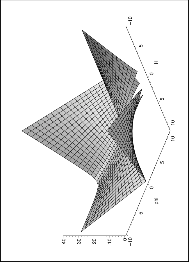
Figure 1: The upper sheet of the “energy surface” corresponding to the positive sign in Eq. (3.80).

As an example, consider the parameter values $\omega=55$ and $\beta=4$ and use units in which $V_{0}$ is unity. Then the region forbidden to the orbits of the solutions is given by

$$|H|<\sqrt{\frac{55}{339}}\,\phi^{1/2}\,.$$ (3.83)

The two sheets composing the “energy surface” have equations

$$\dot{\phi}_{\pm}\left(H,\phi\right)=\frac{3H\phi}{55}\pm\frac{\sqrt{339H^{2}\phi^{2}-55\phi^{3}}}{55}\,.$$ (3.84)

Upper sheet, lower sheet, and the “energy surface” are plotted in Figs. 1-3.

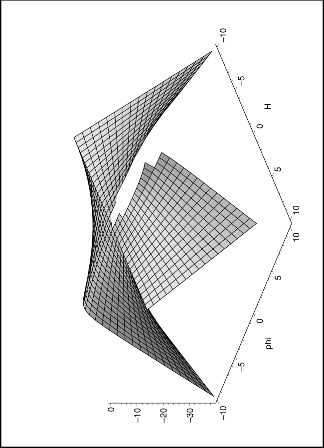
Figure 2: The lower sheet of the “energy surface” corresponding to the negative sign in Eq. (3.80).

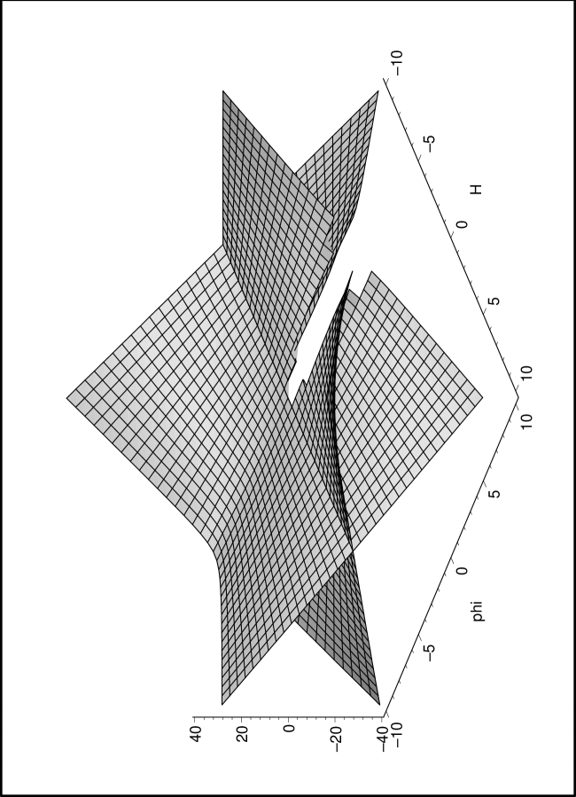
Figure 3: The “energy surface”.

The boundary of the hole, where the two sheets join, is the curve whose points have coordinates

$$\left(H,\phi,\dot{\phi}\right)=\left(\pm\sqrt{\frac{55}{339}}\,\phi^{1/2},\phi,\pm\sqrt{\frac{3}{6215}}\phi^{3/2}\right)\,.$$ (3.85)

The intersections between the energy surface (3.84) and the surface $\dot{\phi}\left(H,\phi\right)=pH\phi$ change as $p$ changes. However, only the value of $p$ given by Eq. (2.41), that is $p=-4/115$ for this example, corresponds to actual orbits of the solutions of the dynamical system (1.8)-(1.10). This “ansatz surface” and its intersection with the “energy surface” are plotted in Fig. 4 and Fig. 5, respectively.

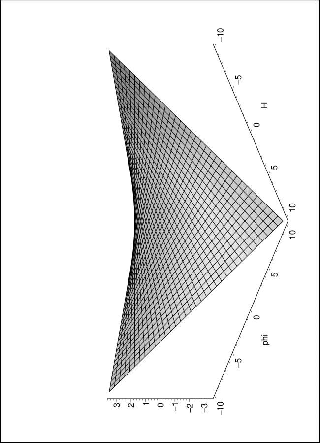
Figure 4: The “ansatz surface” $\dot{\phi}=pH\phi$ corresponding to the assumption $\phi=\phi_{0}a^{p}$.

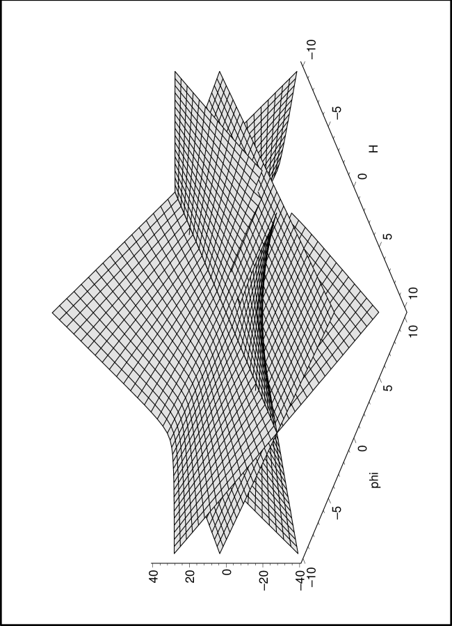
Figure 5: The intersection between the “energy surface” and the “ansatz surface”.

4 Solutions of metric $f(R)$ gravity

$f(R)$ theories of gravity [77, 78] are a subclass of scalar-tensor gravity with action

$$S=\int d^{4}x\,\frac{\sqrt{-g}}{16\pi}\,f(R)+S_{(m)}\,,$$ (4.86)

where $f({\cal R})$ is a non-linear function of the Ricci scalar $R$. This action is equivalent to a Brans-Dicke one. By defining the scalar field $\phi=f^{\prime}(R)$, it can be shown that the action (4.86) is equivalent to [3, 4, 5, 6]

$$S=\int d^{4}x\,\frac{\sqrt{-g}}{16\pi}\left[\phi R-V(\phi)\right]+S_{(m)}\,,$$ (4.87)

where

$$V(\phi)=\phi R(\phi)-f\left(R(\phi)\right)\,,$$ (4.88)

and where $R=R(\phi)$ is now a function of $\phi=f^{\prime}(R)$ usually defined implicitly [3, 4, 5]. This theory has Brans-Dicke coupling $\omega=0$ and the potential (4.88) for the Brans-Dicke scalar.

The Jordan frame solutions of Brans-Dicke cosmology reported in the previous sections can be seen also as solutions of some $f(R)$ cosmology. This is true if $\omega=0$ and

$$V_{0}\left[f^{\prime}(R)\right]^{\beta}=Rf^{\prime}(R)-f(R)\,.$$ (4.89)

The functional form $f(R)=\mu R^{n}$, where $\mu$ and $n$ are constants, satisfies these requirements provided that

$$\beta=\frac{n}{n-1}\,,$$ (4.90)

$$V_{0}=\frac{n-1}{n^{\frac{n}{n-1}}}\,\frac{1}{\mu^{\frac{1}{n-1}}}\,,$$ (4.91)

for $n\neq 1$ (if $n=1$ this $f(R)$ theory reduces to GR). It must be $n>1$ to guarantee that $V_{0}>0$. In practice, the value of $n$ is severely constrained by Solar System experiments, which require that $n=1+\delta$ with $\delta=\left(-1.1\pm 1.2\right)\cdot 10^{-5}$ [80, 81, 82, 83, 84, 85, 86, 87, 88, 89]. At the same time, any $f(R)$ theory must satisfy $f^{\prime}>0$ in order for the graviton to carry positive energy and $f^{\prime\prime}\geq 0$ to guarantee local stability [3, 4, 5, 90]. These constraints are satisfied if $n=1+\delta$ with $\delta\geq 0$. In spite of the experimental bounds on the exponent $n$, $R^{n}$ gravity has been the focus of much work aiming at exploring the possible phenomenology of $f(R)$ gravity and many phase space analyses for $R^{n}$ cosmology are available in the literature [91, 92, 93, 94, 95, 96, 97, 98, 99, 100, 101, 102, 103, 104, 105, 106, 107, 108, 109] (see [113] for a phase space picture of general $f(R)$ cosmology analogous to that of the previous section). Moreover, in strong curvature regimes in the early universe, in which the present-day Solar System constraints do not apply, Starobinsky-like inflation [114] corresponding to $f(R)=R+\mu R^{2}$ is well approximated by $f(R)\simeq\mu R^{2}$.

When the conditions (4.90) and (4.91) are satisfied, the FLRW solutions of Brans-Dicke gravity with power-law potential reported in the previous sections are also solutions of $R^{n}$ gravity with or without a perfect fluid, which are added to the relatively scarce catalogue of exact solutions of these theories.

5 Conclusions

The simple ansatz $\phi=\phi_{0}a^{p}$ recovers most of the known solutions of Brans-Dicke cosmology and generates new ones in the presence of a power-law or inverse power-law potential, which is well-motivated in cosmology and particle physics. These solutions include power-law and exponential dependence of the scale factor $a(t)$ and of the Brans-Dicke field $\phi(t)$ from the comoving time $t$. This ansatz has a fairly simple geometric interpretation in the phase space of the solutions as the simultaneous search for a curve generated by the intersection of two surfaces and for the number $p$. The geometry of the phase space, however, can be complicated for various choices of the (inverse) power-law potential $V(\phi)=V_{0}\phi^{\beta}$ and if the spatial sections of the Brans-Dicke cosmology are curved. Details such as the integration constants appearing in the classic solutions as functions of the parameters of the theory have been provided by new general formulas, which are missing in the literature probably because of the non-availability of computer algebra at the time when these solutions were discovered. We have now a more unified and comprehensive view of analytical solutions of Brans-Dicke cosmology.

Prompted by the huge literature on $f(R)$ cosmology as an alternative to dark energy, it is natural to try to relate the old and new solutions of Brans-Dicke cosmology to corresponding solutions of $f(R)$ cosmology. It turns out that this is possible, and indeed relatively straightforward, for the family described by the choice $f(R)=\mu R^{n}$. The search for new $f(R)$ cosmologies will be continued in the future.

Appendix A

We have three different ways to balance the four terms in the Friedmann equation

$$\underbrace{\frac{q^{2}}{t^{2}}\left(1+p-\frac{\omega p^{2}}{6}\right)}_{(1)}+\underbrace{\frac{k}{a_{0}^{2}\ t^{2q}}}_{(2)}=\underbrace{\frac{8\pi\rho_{0}}{3a_{0}^{p+3\gamma}\phi_{0}}\,\frac{1}{t^{q(p+3\gamma)}}}_{(3)}+\underbrace{\frac{V_{0}\phi_{0}^{\beta-1}}{6\ a_{0}^{p(1-\beta)}}\,\frac{1}{t^{pq(1-\beta)}}}_{(4)}\,:$$ (1.92)

• $(1)$ balances $(3)$, which gives $q(p+3\gamma)=2$, while $(2)$ balances $(4)$, which yields $pq(\beta-1)=2q$. Therefore, it is

  $$p=\frac{2}{1-\beta}\quad\mbox{and}\quad q=\frac{2(1-\beta)}{2+3\gamma(1-\beta)}\,,$$ (1.93)

  and substituting these values into Eq. (1.92), one obtains

  $$\Bigg{\{}\frac{-2\omega+3(\beta-1)(\beta-3)}{\Big{[}2-3\gamma(\beta-1)\Big{]}^{2}}-\frac{2\pi\rho_{0}\,a_{0}^{\frac{2-3\gamma(\beta-1)}{\beta-1}}}{\phi_{0}}\Bigg{\}}\frac{4}{3t^{2}}=\frac{\Big{(}V_{0}\,\phi_{0}^{\beta-1}-6k\Big{)}}{6a_{0}^{2}}\frac{1}{t^{\frac{-4(\beta-1)}{2-3\gamma(\beta-1)}}}\,.$$ (1.94)

  Equating to zero the terms in parenthesis separately yields

  $$\rho_{0} = \frac{-2\omega+3(\beta-1)(\beta-3)}{2\pi\Bigg{[}2-3\gamma(\beta-1)\Bigg{]}^{2}}\phi_{0}\,a_{0}^{\frac{-2+3\gamma(\beta-1)}{\beta-1}}\,,$$ (1.95)

  $$k = \frac{V_{0}\phi^{\beta-1}}{6}\,.$$

  If we substitute these $\rho_{0}$ and $k$ values into the acceleration equation (1.9), we obtain

  $$\left(-3+2\omega+3\beta\right)\Bigg{\{}\frac{12\big{[}2-4\beta+2\omega(\gamma-2)+3\gamma(\beta-1)\big{]}}{(2-3\gamma(\beta-1))^{2}t^{2}}+\frac{V_{0}\phi_{0}^{\beta-1}}{a_{0}^{2}t^{\frac{-4(\beta-1)}{2-3\gamma(\beta-1)}}}\Bigg{\}}=0\,.$$ (1.97)

  This equation can be satisfied in two ways: the first one consists of setting the first parenthesis to zero, while the second way consists of setting the second parenthesis to zero. However, the second possibility is already discussed in Sec. 2.7. Setting the first parenthesis to zero gives

  $$\beta=\frac{3-2\omega}{3}\,.$$ (1.98)

  Now we need to satisfy the scalar field equation (1.10), which gives

  $$\frac{2a_{0}^{2}(2\omega+3)}{t^{2}}-\frac{V_{0}\,\phi_{0}^{-\frac{2\omega}{3}}(\omega\gamma+1)^{2}}{t^{\frac{4\omega}{3(\omega\gamma+1)}}}=0\,,$$ (1.99)

  requiring one to set the powers of $t$ equal to each other. Therefore, we conclude that balancing these two pairs does not produce any new solution.

• Balancing the terms $(2)$ and $(3)$ gives $2q=q(p+3\gamma)$, whereas balancing $(1)$ and $(4)$ yields $pq(1-\beta)=2$, therefore

  $$p=2-3\gamma\quad\mbox{and}\quad q=\frac{2}{(3\gamma-2)(\beta-1)}\,,$$ (1.100)

  while the Friedmann equation (1.92) gives

  $$\Bigg{\{}\frac{4[\omega(3\gamma-2)^{2}+18(\gamma-1)]}{(3\gamma-2)^{2}(\beta-1)^{2}}+\frac{V_{0}\,\phi_{0}^{\beta-1}}{a_{0}^{(\beta-1)(3\gamma-2)}}\Bigg{\}}\frac{1}{t^{2}}=\frac{3k\,\phi_{0}-8\pi\,\rho_{0}}{a_{0}^{2}\phi_{0}}\frac{2}{t^{\frac{4}{(\beta-1)(3\gamma-2)}}}\,,$$ (1.101)

  which implies that

  $$V_{0} = -\frac{4\,a_{0}^{(\beta-1)(3\gamma-2)}[\omega(3\gamma-2)^{2}+18(\gamma-1)]}{\phi_{0}^{\beta-1}(3\gamma-2)^{2}(\beta-1)^{2}}\,,$$ (1.102)

  $$k = \frac{8\pi\,\rho_{0}}{3\phi_{0}}\,.$$ (1.103)

  If we substitute these values of $V_{0}$ and $k$ into the acceleration equation (1.9), we obtain

  $$\left[3+\omega(3\gamma-2)\right]\Bigg{\{}\frac{6(2\omega+2\beta-1)-9\gamma(2\omega+\beta+1)}{(3\gamma-2)^{2}(\beta-1)^{2}\,t^{2}}-\frac{4\pi\,\rho_{0}}{a_{0}^{2}\phi_{0}\,t^{\frac{4}{(\beta-1)(3\gamma-2)}}}\Bigg{\}}=0\,.$$ (1.104)

  A possible solution would be obtained if the prefactor $\left[3+\omega(3\gamma-2)\right]$ vanishes, giving

  $$\gamma=\frac{2\omega-3}{3\omega}\,.$$ (1.105)

  In order to satisfy the scalar field equation (1.10), we substitute the values of $V_{0}$, $k$, and $\gamma$ to obtain

  $$\frac{\omega(2\omega+3)(\beta+1)}{t^{2}}-\frac{12\pi\,\rho_{0}(\beta-1)^{2}}{a_{0}^{2}\,\phi_{0}\,t^{\frac{-4\omega}{3(\beta-1)}}}=0\,.$$ (1.106)

  Finding a solution without setting the powers of $t$ equal to each other requires, at a minimum, to set $\beta=1$, which makes the power of $t$ infinite. Therefore, this choice of balancing terms give no reasonable solution without setting the powers of $t$ equal to each other.

• Another possible solution of the dynamical equations arises if $(1)$ balances $(2)$, which gives $2q=2$, while $(3)$ balances $(4)$, which yields $q(p+3\gamma)=pq(1-\beta)$. Therefore $q$ and $p$ become

  $$q=1\quad\mbox{and}\quad p=-\frac{3\gamma}{\beta}\,.$$ (1.107)

  Substituting these values of $q$ and $p$ into the Friedmann equation (1.92) leads to

  $$\Bigg{[}\frac{6k}{a_{0}^{2}}-\frac{3(3\omega\gamma^{2}+6\gamma\beta-2\beta^{2})}{\beta^{2}}\Bigg{]}\frac{1}{t^{2}}=\Bigg{[}\frac{16\pi\,\rho_{0}}{\phi_{0}}+V_{0}\phi_{0}^{\beta-1}\Bigg{]}\frac{1}{(a_{0}\,t)^{\frac{3\gamma(\beta-1)}{\beta}}}\,,$$ (1.108)

  which requires

  $$k = \frac{a_{0}^{2}\left(3\omega\gamma^{2}+6\gamma\beta-2\beta^{2}\right)}{2\beta^{2}}\,,$$ (1.109)

  $$\rho_{0} = -\frac{V_{0}\phi_{0}^{\beta}}{16\pi}\,.$$ (1.110)

  Requiring that the energy density and the potential energy density be non-negative, one must set $\rho_{0}=V_{0}=0$. Substituting these values of $k$, $\rho_{0}$, and $V_{0}$ into the acceleration equation (1.9) leads to

  $$3\gamma(\omega\gamma+\beta)=0\,,$$ (1.111)

  and $\gamma$ becomes

  $$\gamma=0\quad\mbox{or}\quad\gamma=-\frac{\beta}{\omega}\,.$$ (1.112)

  We still have to satisfy the scalar field equation (1.10). If we set $\gamma=0$, the scalar field becomes constant, $\phi(t)=\phi_{0}$, which reduces the context to GR. For $\gamma=-\beta/\omega$ one obtains instead

  $$\frac{3a_{0}^{3/\omega}\left(2\omega+3\right)\phi_{0}}{t^{\frac{2\omega-3}{\omega}}\,\omega^{2}}=0\,,$$ (1.113)

  which is satisfied only if $\omega=-3/2$, the unacceptable value of the Brans-Dicke parameter ruled out from the beginning.

These three cases show that making different matches of the terms in Friedmann equation (1.92) does not yield new solutions.

References

• [1] T. Clifton, P.G. Ferreira, A. Padilla, and C. Skordis, Phys. Reports 513, 1189 (2012).
• [2] L. Amendola and S. Tsujikawa, Dark Energy, Theory and Observations (Cambridge University Press, Cambridge, 2010).
• [3] T.P. Sotiriou and V. Faraoni, Rev. Mod. Phys. 82, 451 (2010).
• [4] A. De Felice and S. Tsujikawa, Living Rev. Relativity 13, 3 (2010).
• [5] S. Nojiri and S.D. Odintsov, Phys. Repts. 505, 59 (2011).
• [6] S. Capozziello and V. Faraoni, Beyond Einstein Gravity (Springer, New York, 2010).
• [7] C.H. Brans and R.H. Dicke, Phys. Rev. 124, 925 (1961).
• [8] P.G. Bergmann, Int. J. Theor. Phys. 1, 25 (1968).
• [9] R.V. Wagoner, Phys. Rev. D 1, 3209 (1970).
• [10] K. Nordvedt, Astrophys. J. 161, 1059 (1970).
• [11] E. Berti et al., Class. Quantum Grav. 32, 243001 (2015).
• [12] T. Baker, D. Psaltis, and C. Skordis, Astrophys. J. 802, 63 (2015).
• [13] C.G. Callan, D. Friedan, E.J. Martinez, and M.J. Perry, Nucl. Phys. B 262, 593 (1985).
• [14] E.S. Fradkin and A.A. Tseytlin, Nucl. Phys. B 261, 1 (1985).
• [15] V. Faraoni, Cosmology in Scalar-Tensor Gravity (Kluwer Academic, Dordrecht, 2004).
• [16] Y. Fujii and K. Maeda, The Scalar-Tensor Theory of Gravity (Cambridge University Press, Cambridge, 2003).
• [17] D. La and P.J. Steinhardt, Phys. Rev. Lett. 62, 376 (1989).
• [18] E.J. Weinberg, Phys. Rev. D 40, 3950 (1989).
• [19] D. La, P.J. Steinhardt, and E. Bertschinger, Phys. Lett. B 231, 231 (1989).
• [20] A.R. Liddle and D. Wands, Mon. Not. Roy. Astr. Soc. 253, 637 (1991).
• [21] F.S. Accetta and J.J. Trester, Phys. Rev. D 39, 2854 (1989).
• [22] D. La, P.J. Steinhardt and E. Bertschinger, Phys. Lett. B 231, 231 (1989).
• [23] R. Holman, E.W. Kolb, and Y. Wang, Phys. Rev. Lett. 65, 17 (1990).
• [24] R. Holman, E.W. Kolb, S. Vadas, and Y. Wang, Phys. Lett. B 269, 252 (1991).
• [25] A.M. Laycock and A.R. Liddle, Phys. Rev. D 49, 1827 (1994).
• [26] J. McDonald, Phys. Rev. D 48, 2462 (1993).
• [27] T. Chiba, Phys. Rev. D 60, 083508 (1999).
• [28] J.-P. Uzan, Phys. Rev. D 59, 123510 (1999).
• [29] F. Perrotta, C. Baccigalupi, and S. Matarrese, Phys. Rev. D 61, 023507 (2000).
• [30] L. Amendola, Mon. Not. R. Astr. Soc. 312, 521 (2000).
• [31] R. de Ritis, A.A. Marino, and P. Scudellaro, Phys. Rev. D 62, 043506 (2000).
• [32] X. Chen, R.J. Scherrer, and G. Steigman, Phys. Rev. D 63, 123504 (2001).
• [33] G. Esposito-Farése, gr-qc/0011115.
• [34] A.A. Sen and R.T. Seshadri, Int. J. Mod. Phys. D 12, 445 (2000).
• [35] C. Baccigalupi, S. Matarrese, and F. Perrotta, Phys. Rev. D 62, 123510 (2000).
• [36] Y. Fujii, Gravit. Cosmol. 6, 107 (2000).
• [37] Y. Fujii, Phys. Rev. D 62, 044011 (2000).
• [38] O. Bertolami and J. Martins, Phys. Rev. D 61, 064007 (2000).
• [39] L. Amendola, Phys. Rev. D 62, 043511 (2000).
• [40] L. Amendola, Phys. Rev. Lett. 86, 196 (2001).
• [41] B. Boisseau, G. Esposito-Farése, D. Polarski, and A.A. Starobinski, Phys. Rev. Lett. 85, 2236 (2000).
• [42] M.C. Bento, O. Bertolami, and N.C. Santos, Phys. Rev. D 65, 067301 (2002).
• [43] T. Chiba, Phys. Rev. D 64, 103503 (2001).
• [44] A. Riazuelo and J.-P. Uzan, Phys. Rev. D 62, 083506 (2000).
• [45] G. Esposito-Farése and D.Polarski, Phys. Rev. D 63, 063504 (2001).
• [46] N. Banerjee and D. Pavon, Class. Quant. Grav. 18, 593 (2001).
• [47] V. Faraoni, Int. J. Mod. Phys. D 11, 471 (2002).
• [48] D.F. Torres, Phys. Rev. D 66, 043522 (2002).
• [49] F. Perrotta and C. Baccigalupi, Nucl. Phys. Proc. Suppl. 124, 68 (2003).
• [50] A. Riazuelo and J.-P. Uzan, Phys. Rev. D 66, 023535 (2002).
• [51] S. Nojiri and S.D. Odintsov, Phys. Rev. D 68, 123512 (2003).
• [52] E. Elizalde et al., Phys. Lett. B 574, 1 (2003).
• [53] E. Elizalde, S. Nojiri and S.D. Odintsov, Phys. Rev. D 70, 043539 (2004).
• [54] S. Nojiiri and S.D. Odintsov, Phys. Lett. B 595, 1 (2004).
• [55] S. Matarrese, C. Baccigalupi, and F. Perrotta, Phys. Rev. D 70, 061301 (2004).
• [56] R. Catena et al., astro-ph/0406152.
• [57] F.C. Carvalho and A. Saa, Phys. Rev. D 70, 087302 (2004).
• [58] W. Chakraborty and U. Debnath, Int. J. Theor. Phys. 48, 232247 (2009).
• [59] R.M. Wald, General Relativity (Chicago University Press, Chicago, 1984).
• [60] L. Pietronero, E. Tosatti, V. Tosatti, and A. Vespignani, Phys. A 293, 297 (2001).
• [61] J. Huxley and G. Teissier, Nature 137, 780 (1936).
• [62] J. Gayon, Am. Zool. 40, 748 (2000).
• [63] R. Horton, Geol. Soc. Am. Bull. 56, 275 (1945).
• [64] A. Strahler, Civ. Eng. 101, 1258 (1980).
• [65] P. Dodds and D. Rothman, Annu. Rev. Earth. Planet. Sci. (28) 571 (2000).
• [66] D. Bahr, W.T. Pfeffer, and G. Kaser, Rev. Geophys. 53, 95 (2015).
• [67] C.M. Will, Living Rev. Relativ. 17, 4 (2014).
• [68] F. Accetta, L. Krauss, and P. Romanelli, Phys. Lett. B 248, 146 (1990).
• [69] J. O’Hanlon and B. Tupper, Nuovo Cimento B 7, 305 (1972).
• [70] H. Nariai, Prog. Theor. Phys. 40, 49 (1968).
• [71] L.E. Gurevich, A.M. Finkelstein, and V.A. Ruban, Astrophys. Sp. Sci. 22, 231 (1973).
• [72] J.D. Barrow and K. Maeda, Nucl. Phys. B 341, 294 (1990).
• [73] C. Romero and A. Barros, Gen. Rel. Grav. 23, 491 (1993).
• [74] S.J. Kolitch, Ann. Phys. (NY) 246, 121 (1996).
• [75] V. Mukhanov, Physical Foundations of Cosmology (Cambridge University Press, Cambridge, 2005).
• [76] V. Faraoni, Ann. Phys. (NY) 317, 366 (2005).
• [77] S. Capozziello, S. Carloni, and A. Troisi, Recent Res. Dev. Astron. Astrophys. 1, 625 (2003).
• [78] S.M. Carroll, V. Duvvuri, M. Trodden, and M.S. Turner, Phys. Rev. D 70, 043528 (2004).
• [79] S.H. Hendi, Phys. Lett. B 690, 220 (2010).
• [80] T. Clifton, Class. Quantum Grav. 23, 7445 (2006).
• [81] J.D. Barrow and T. Clifton, Class. Quantum Grav. 23, L1 (2005).
• [82] T. Clifton and J.D. Barrow, Phys. Rev. D 72, 103005 (2005).
• [83] T. Clifton and J.D. Barrow, Class. Quantum Grav. 23, 2951 (2005).
• [84] A.F. Zakharov, A.A. Nucita, F. De Paolis, and G. Ingrosso, Phys. Rev. D 74, 107101 (2006).
• [85] A. Abebe, A. de la Cruz-Dombriz, and P.K.S. Dunsby, Phys. Rev. D 88, 044050 (2013).
• [86] A. Abebe, M. Abdelwahab, A. de la Cruz-Dombriz, and P.K.S Dunsby, Class. Quantum Grav. 29, 135011 (2012).
• [87] M. Aparicio Resco, A. de la Cruz-Dombriz, F.J. Llanes Estrada, and V. Zapatero Castrillo, Phys. Dark Universe 134, 147 (2016).
• [88] A.V. Astashenok and S.D. Odintsov, Phys. Rev. D 94, 063008 (2016).
• [89] P. Salucci, C. Frigerio Martins, and E. Karukes, Int. J. Mod. Phys. D 23, 1442005 (2014).
• [90] V. Faraoni, Phys. Rev. D 74, 104017 (2006).
• [91] H.R. Kausar, Eur. Phys. J. C 77, 374 (2017).
• [92] C. van de Bruck, P. Dunsby, and L.E. Paduraru, Int. J. Mod. Phys. D 26, 1750152 (2017).
• [93] M. Abdelwahab, A. de la Cruz-Dombriz, P.K.S. Dunsby, and B. Mongwane, arXiv:1412.6350.
• [94] A. de la Cruz-Dombriz, P.K.S. Dunsby, V.C. Busti, and S. Kandhai, Phys. Rev. D 89, 064029 (2014).
• [95] L.G. Jaime, L. Patiño, M. Salgado, Phys. Rev. D 87, 024029 (2013).
• [96] A. Abebe, A. de la Cruz-Dombriz, and P.K.S. Dunsby, Phys. Rev. D 88, 044050 (2013).
• [97] T. Clifton, P. Dunsby, R. Goswami, A.M. Nzioki, Phys. Rev. D 87, 063517 (2013).
• [98] M. Abdelwahab, R. Goswami, and P.K.S. Dunsby, Phys. Rev. D 85, 083511 (2012).
• [99] M. Abdelwahab, R. Goswami, and P.K.S. Dunsby, AIP Conf. Proc. 1458, 303 (2011).
• [100] A.M. Nzioki, P.K.S. Dunsby, R. Goswami, and S. Carloni, Phys. Rev. D 83, 024030 (2011).
• [101] V. Faraoni, Phys. Rev. D 83, 124044 (2011).
• [102] K.N. Ananda, S. Carloni, and P.K.S. Dunsby, Springer Proc. Phys. 137, 165 (2011).
• [103] N. Goheer, J. Larena, and P.K.S. Dunsby, Phys. Rev. D 80, 061301 (2009).
• [104] S. Carloni, P.K.S. Dunsby, and A. Troisi, arXiv:0906.1998.
• [105] A. Aviles Cervantes, J.L. Cervantes-Cota, AIP Conf. Proc. 1083, 57 (2008).
• [106] N. Goheer, J.A. Leach, P.K.S. Dunsby, Class. Quantum Grav. 24, 5689 (2007).
• [107] V. Faraoni and S. Nadeau, Phys. Rev. D 72, 124005 (2007).
• [108] J.A. Leach, S. Carloni, and P.K.S. Dunsby, Class. Quantum Grav. 23, 4915 (2006).
• [109] S. Carloni, P.K.S. Dunsby, S. Capozziello, A. Troisi, Class. Quantum Grav. 22, 4839 (2005).
• [110] S. Carloni, P. Dunsby, S. Capozziello, and A. Troisi, Class. Quantum Grav. 22, 4839 (2005).
• [111] S. Nojiri, S.D. Odintsov, and S. Ogushi, Phys. Rev. D 65, 023521 (2002).
• [112] S. Nojiri and S.D. Odintsov, Phys. Rev. D 68, 123512 (2003).
• [113] J.C.C. de Souza and V. Faraoni, Class. Quantum Grav. 24, 3637 (2007).
• [114] A.A. Starobinsky, Phys. Lett. B 91, 99 (1980).