Dynamical Origin and Terrestrial Impact Flux
of Large Near-Earth Asteroids

Abstract

Dynamical models of the asteroid delivery from the main belt suggest that the current impact flux of diameter $D>10$ km asteroids on the Earth is $\simeq 0.5$-1 Gyr^-1. Studies of the Near-Earth Asteroid (NEA) population find a much higher flux, with $\simeq$7 $D>10$-km asteroid impacts per Gyr. Here we show that this problem is rooted in the application of impact probability of small NEAs ($\simeq 1.5$ Gyr^-1 per object), whose population is well characterized, to large NEAs. In reality, large NEAs evolve from the main belt by different escape routes, have a different orbital distribution, and lower impact probabilities ($0.8\pm 0.3$ Gyr^-1 per object) than small NEAs. In addition, we find that the current population of two $D>10$ km NEAs (Ganymed and Eros) is a slight fluctuation over the long term average of $1.1\pm 0.5$ $D>10$ km NEAs in a steady state. These results have important implications for our understanding of the occurrence of the K/T-scale impacts on the terrestrial worlds.

1 Introduction

The impact cratering record of the Moon and terrestrial planets provides important clues about the impactor flux in the inner Solar System. The number of craters recorded on each world’s surface is a measure of the intensity of the bombardment that the surface experienced over its age. If the surface age is known, the crater data can be interpreted to yield clues about the nature of the impactor population. If the impactor population is well characterized from independent means, the crater data can be used to estimate the surface age. It is often the case, however, that both the surface age and the properties of the impactor population are uncertain, leaving us with a difficult task mathematically equivalent to one equation with two unknowns. Things are further complicated by uncertainties in the scaling laws that are used to calculate the crater size from the impactor’s mass and velocity (e.g., Holsapple 1993, Johnson et al. 2016).

Historically, the problem of interpreting crater records on different worlds has been approached from two different angles. In the first approach, which is firmly set in the realm of data-driven science, the crater counts are obtained from the existing imagery and used to define the so-called production function, which, apart from uncertainties in the scaling laws, conveys the size and time dependence of the impactor population (e.g., Neukum et al. 2001, Hartmann & Neukum 2001, Marchi et al. 2012, Robbins 2014). The results of crater counts are often correlated among different worlds to demonstrate the applicability, or the lack of it, of the production function in different parts of the Solar System, and during different epochs of the Solar System history.

The second, theory-driven approach strives to understand the impactor population by modeling the orbital evolution and estimating the impact probabilities (e.g., Bottke et al. 2002, 2012; Morbidelli et al. 2002; Minton & Malhotra 2010; Nesvorný et al. 2017). A theoretical model expresses our expectations about the impact flux on different worlds and its time variability. It is often calibrated on telescopic observations of small-body populations (e.g., near-Earth asteroids), and thus represents a useful link between different datasets (e.g., between crater counts and telescopic observations of NEAs and main belt asteroids).

Each of the methods described above has its shortcomings. The data-driven approach yields a crater production function but does not tell us, at least not immediately, the meaning of the cratering record in the context of the known Solar System architecture (e.g., the source of impactors). The modeling approach, on the other hand, can struggle to accurately represent the reality, because the populations of small bodies may not be well characterized from observations, especially at small sizes, or because the computer simulations may not be accurate (poor resolution due to CPU limitations, uncertain nature of dynamical processes, etc.). These and other issues often lead to a situation where inconsistencies arise between the model expectations and data-based inferences about the impactor flux.

2 Motivating Problem

Here we aim at resolving one such inconsistency related to the present-day impact flux in the inner Solar System. Stated briefly, the problem arises when one compares the impact flux inferred from analysis of NEAs with the impact flux obtained from dynamical models of NEA delivery from the main asteroid belt. For example, Johnson et al. (2016) reported, adopting the former approach and assuming that the NEA impact flux was constant over the past 1 Gyr, that $\simeq 7$ impacts of $D>10$-km asteroids should have occurred on the Earth in the last 1 Gyr. A similar value was previously reported in many other publications, including Chapman & Morrison (1994), Stuart & Binzel (2004), Le Feuvre & Wieczorek (2011) and Harris & D’Abramov (2015). In contrast, Nesvorný et al. (2017) estimated from their dynamical modeling that only $\sim$0.5-1 such impacts should occur. The model impact rates are therefore $\sim$7-14 times below expectations. A similar discrepancy was noted in Minton & Malhotra (2010), who compared their model results with Neukum’s production function (Neukum et al. 2001).

This can mean one of several things. First, the current-day impactor flux may be, for some reason, larger than the average flux over the past Gyr (e.g., Culler et al. 2000, Mazrouei et al. 2017). Alternatively, some model parameters in Nesvorný et al. (2017) and Minton & Malhotra (2010) may need to be tweaked to increase the computed impact flux in the last 1 Gyr. It is not clear, however, how this can be done, because the impact flux in the last 1 Gyr was shown to be nearly independent, to within a factor of $\sim$2, of various model parameters (such as history of planetary orbits, distribution of main belt asteroids, etc.; see discussion in Nesvorný et al. 2017). The uncertainties in the model thus do not appear to be responsible for the identified problem. Here we demonstrate, instead, that the problem appears because the NEA-based estimate of the impact flux of large asteroids in the works cited above is inaccurate.

To estimate the impact rate, the NEA-based studies assumed that the impact probability of large NEAs is essentially the same as the impact probability of small NEAs. Consequently, they used an average value for the NEA impact probability, and the size distribution of NEAs, to compute the current impact flux of asteroids with $1<D<10$ km. The impact flux was extrapolated to $D>10$ km using the size distribution of main belt asteroids. This approach is adequate for impactors with $D\sim 1$ km, where the NEA size and orbital distributions are well characterized. It may not be fully appropriate, however, to extrapolate the results to large asteroids, because it is not guaranteed that the orbital distribution of large NEAs and their impact probabilities are the same (see, e.g., Valsecchi & Gronchi 2011).

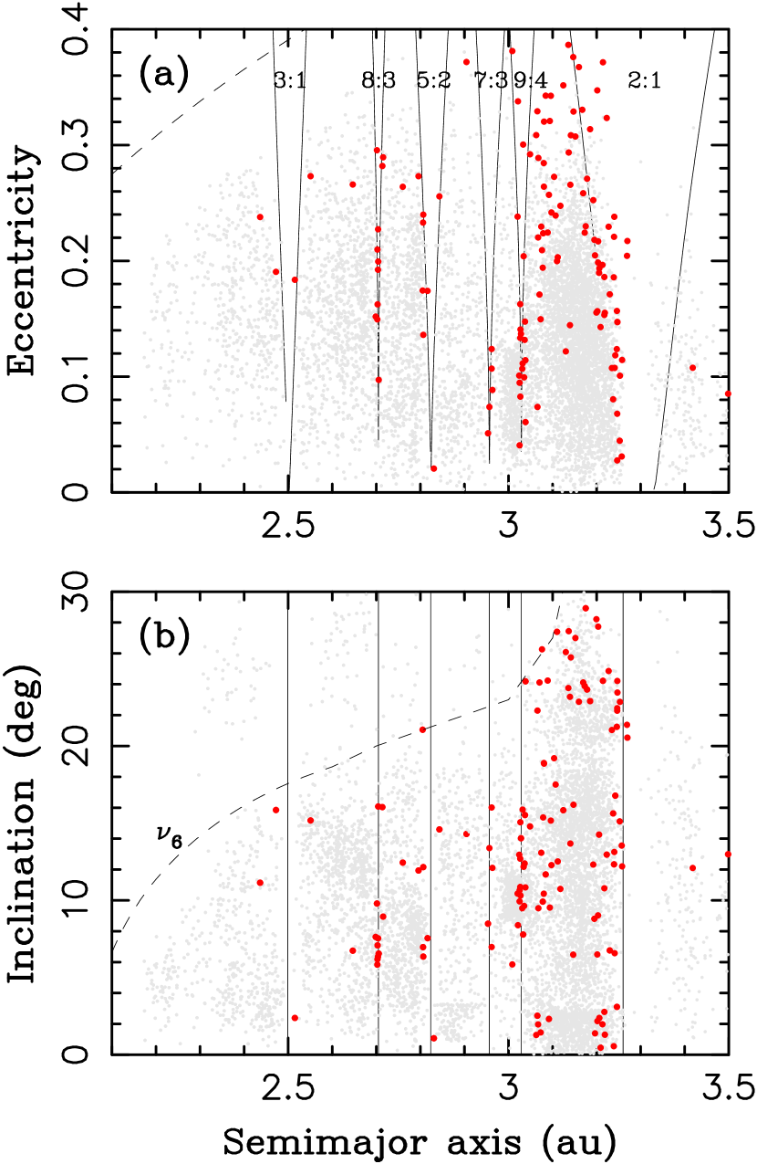
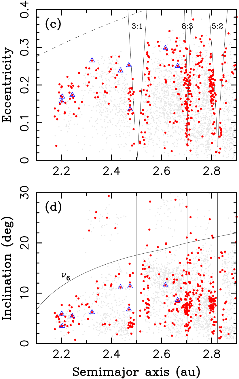
Figure 1: Panels (a) and (b): The initial orbits of $D>10$ km main belt asteroids that remained in the main belt at 100 Myr after the start of our integration (gray dots) and those that escaped from the belt in 100 Myr (red dots). Only the clones with zero Yarkovsky drift were considered in the plot on the left. Panels (c) and (d): A zoom in on the inner part of the belt. Here we used the full length of the integration (1 Gyr) and all 15 clones. The triangles denote asteroids that ended up impacting on the terrestrial planets. The thin solid lines denote the location of orbital resonances. The thin dashed line in (a) and (c) is the Mars crossing limit.

On one hand, large asteroids typically reach the NEA orbits via slow diffusion in weak resonances (Migliorini et al. 1998, Morbidelli & Nesvorný 1999, Farinella & Vokrouhlický 1999). The small asteroids, on the other hand, can drift over a considerable radial distance by the Yarkovsky effect and reach NEA space from the powerful $\nu_{6}$ resonance at the inner edge of the asteroid belt (Bottke et al. 2002). The $\nu_{6}$ resonance is known to produce highly evolved NEA orbits and impact probabilities on Earth in excess of 1% (Gladman et al. 1997). The small NEAs can therefore have larger impact probabilities than the large ones (Valsecchi & Gronchi 2015). If correct, this would imply that the current impact flux should drop more steeply with impactor size (see, e.g., Fig. 1 in Johnson et al. (2016) or Fig. 5 in Harris & D’Abramov (2015)), therefore implying fewer than $\simeq 7$ $D>10$-km asteroid impacts in the last 1 Gyr.

It is difficult to test this conjecture based on the NEA population alone, because there are not enough $D>10$ km NEAs, and the statistical inferences based on them would not produce robust results. The dynamical model of Nesvorný et al. (2017) also cannot be used to resolve this problem with confidence, because several model approximations make it a less than ideal gauge of the current impact flux (the model was developed to study the dependence of the historical impact flux of planetary impactors under different assumptions). For example, the main belt structure was not exactly reproduced in Nesvorný et al. (2017). In addition, their simulations neglected the Yarkovsky effect. According to Bottke et al. (2006), the maximum Yarkovsky drift rate of a $D=10$-km inner-belt asteroid is $\simeq 2\times 10^{-5}$ au Myr^-1. Thus, the expected maximum drift over 1 Gyr is roughly 0.02 au. This seems small but should be significant, because weak diffusive resonances in the inner main belt, which provide the main escape routes for large asteroids, are very dense, and the nearest one may be only a tiny fraction of an au away. It is therefore important to include the Yarkovsky effect to do things correctly.

The Yarkovsky effect also appears to be responsible for the related problem reported in Minton & Malhotra (2010). They performed simulations of the main belt asteroids without the Yarkovsky effect, calibrated their model on the number of large asteroids remaining in the belt today, and found that on average $\sim$1 $D>10$ km asteroids should have impacted on Earth in the last Gyr. Note that this estimate is consistent, to within a factor of 2, with the one derived from a similar model in Nesvorný et al. (2017), but $\sim$7 times lower than the one reported in Johnson et al. (2016). The reason why they obtained a slightly higher impact flux than in Nesvorný et al. (2017) is probably related to the fact that Minton & Malhotra (2010) did not account for the early planetary migration/instability which acted to deplete the inner part ($a<2.5$ au) of the main belt (Nesvorný et al. 2017). Their model may thus slightly overestimate the impact flux, because the inner belt, which produces most NEA impactors, is more populated in their model than in reality (see Figure 4 in Minton & Malhotra 2010).

Minton & Malhotra (2010) compared the impact flux obtained in their work with the Neukum production function (Neukum et al. 2001) and found that, when the production function is applied to large impactors, it predicts $\simeq$6-18 terrestrial impacts of $D>10$ km asteroids in the last 1 Gyr. Neukum and collaborators, however, developed their production function mainly from the analysis of counts of small recent craters that were produced by $D\ll 10$ km projectiles, for which the Yarkovsky effect is very important (e.g., Granvik et al. 2017). To link this to large impactors, they had to use the crater counts on older terrains, because craters produced by large projectiles are rare in the recent Solar System history. To calculate the recent impact flux of large asteroids from this exercise, the knowledge of the time dependence of the impactor flux is required.

But here it is not expected that the time dependence of crater production rate over the past $\sim$4 Gyr was the same for small and large impactors. This is because the dynamical delivery of impactors during the early epochs was controlled by size-independent dynamical processes (e.g., Nesvorný et al. 2017). At the present time, instead, the impactor delivery from the main belt is regulated by the size-dependent Yarkovsky effect (see, e.g., Strom et al. 2005). Most small NEA impactors, for example, evolve from the main belt by drifting into the $\nu_{6}$ resonance (Bottke et al. 2002, Granvik et al. 2017). Consequently, they have higher impact probabilities (normalized to one object) on the terrestrial worlds than large asteroids, which reach the NEA orbits via different escape routes (see below).

The time dependence (chronology) of the impactor flux in Neukum et al. (2001) was constructed from small craters/impactors and therefore has the Yarkovsky effect in it. It is not obvious how to extrapolate the current impact flux it predicts to large impactors, which are affected by the Yarkovsky effect to a lesser degree. It would also be strictly incorrect to use the counts of large craters on ancient lunar terrains and extrapolate them to recent times with the time dependence of the production function extracted from small crater counts. In fact, the impactor flux of large asteroids on the terrestrial worlds must have dropped more steeply from $\sim 4$ Gyr ago to present than the Neukum production function would suggest. This is likely the source of the order-of-magnitude discrepancy discussed above.

3 Methods

We used the Wide-field Infrared Survey Explorer (WISE) catalog (Mainzer et al. 2011) to select all known $D>10$ km main-belt asteroids, 8193 in total, with semimajor axes $2<a<3.5$ au. The known population with WISE-diameter measurement is essentially complete for $D>10$ km. We only consider large asteroids, because: (1) the motivating problem of this work concerns the impact flux of large asteroids, (2) the known population of small main belt asteroids is incomplete and models based on it would suffer from various uncertainties, and (3) the dynamics of small asteroids is affected by the radiation torque known as the YORP effect (Vokrouhlický et al. 2015), whose strength depends on small scale surface features (e.g., Statler 2009) and is difficult to model with confidence (e.g., Bottke et al. 2015).

Three clones were considered for each selected asteroid. The first clone was given the maximal negative Yarkovsky drift rate, the second one was given the maximal positive Yarkovsky drift rate, and the third one was given no drift. The maximal/minimal Yarkovsky drift rates were assigned to each individual body depending on its size and semimajor axis (see, e.g., Bottke et al. 2006). The drift rates were kept fixed during each orbital integration. This is an adequate approximation because the strength of the YORP effect scales as $1/D^{2}$ and quickly drops for large $D$. The obliquity changes due to the (neglected) YORP cycles should therefore be modest. We considered clones with the maximal and minimal drift rates to test how the impact flux depends on the full range of possibilities. Bodies with intermediate drift rates are expected to lead to intermediate results. With three clones for each $D>10$ km asteroid with $2<a<3.5$ au, we have nearly 25,000 bodies in total.

Our numerical integrations included planets, which were treated as massive bodies that gravitationally interact among themselves and affect the orbits of all other bodies, and asteroid clones, which were massless (i.e., they did not affect each other and the planets). The integrations were performed with the Swift $N$-body program (Levison & Duncan 1994), which is an efficient implementation of the symplectic Wisdom-Holman map (Wisdom & Holman 1991). Specifically, we used the code known as swift_rmvs that we adapted for the problem in hand. First, the code was modified such that it can be efficiently parallelized on a large number of CPUs. Second, we modified the treatment of close encounters between planets and asteroid clones such that the evolution of planetary orbits on each CPU is strictly the same (this code is known as swift_rmvs4). Third, we included the Yarkovsky force in the kick part of the integrator.

The collisional evolution was ignored, because $D>10$-km asteroids in the main belt have very long collisional lifetimes ($>$1 Gyr, Bottke et al. 2005; the collisional lifetime is asteroid’s mean lifetime against catastrophic disruption). We did not include the YORP effect in the integrations, because the main effect of YORP should be to produce extreme obliquity values and maximize the Yarkovsky drift, which is accounted for by considering clones with maximal and minimal drift rates (but see Vokrouhlický et al. 2003). The dependence of the results on the YORP cycles could be tested with the stochastic YORP code that has been calibrated on various datasets (Bottke et al. 2015), but this is left for future work. We do not expect any major differences, because the YORP cycles of $D>10$-km main-belt asteroids are very long.

The integrations were performed on NASA’s Pleiades Supercomputer. The integration with 25,000 asteroid clones was split over 2,500 Pleiades cores with each core dealing with 10 clones. All planets except Mercury were included. Leaving out Mercury allowed us to perform the simulations with a reasonably low CPU cost. The gravitational effects of Mercury were found insignificant in previous works (e.g., Granvik et al. 2016). The integration required 120 hours on 500 Pleiades cores. It covered 1 Gyr allowing us to monitor the asteroid impacts on the terrestrial planets during this time. It was run forward from the current epoch such that the results obtained from it should be strictly applicable to the impact flux during the next 1 Gyr. Still, with some uncertainty, the impact flux obtained from our integration can be thought as being representative of that at the present epoch.

The orbital elements of asteroids escaping into NEA space were saved at fixed time intervals and used as an input for an Öpik-style collisional code (e.g., Greenberg 1982, Bottke & Greenberg 1993, Vokrouhlický et al. 2012). The code was used to compute the impact flux on different terrestrial worlds (Venus, Earth, Mars and the Moon). The effects of gravitational focusing were included. The Swift integrator recorded all impacts of asteroid clones on the terrestrial planets that occurred during the integration. This offers an opportunity to compare the number of recorded impacts with the impact profiles obtained from the Öpik code. The results based on the Swift-recorded impacts should be more reliable than the results obtained from the Öpik code, but the statistics from the recorded impact is small (see below). We use the strength of each method to derive the most reliable estimates.

We also performed several additional integrations: (1) with a 1-day step over 100 Myr, and (2) using 15 asteroid clones distributed between the maximum negative and maximum positive values of the Yarkovsky drift. The former simulation was used to validate the nominal simulation with a longer timestep (3 days). We have not detected any statistically significant differences in the impact rate, number of NEAs or any other parameter. Simulation (2) was used to confirm that using clones with intermediate drift rates does not change the results. The increased statistics with 15 clones also helps to produce a larger number of recorded impacts in Swift and guarantee that the statistics derived from the Swift-recorded is reliable.

4 Results

4.1 Escape rate of $D>10$ km asteroids

Figure 1a,b highlights the initial orbits of asteroids that escaped from the main belt in the course of our integration. This figure illustrates a couple of things. First, in what concerns the $D>10$ km bodies, the outer belt represents a much larger population than the inner belt. For example, when we compare the number of $D>10$ km asteroids with $a>2.9$ au and $a<2.9$ au, we find that the outer part of the belt contains more than twice as many asteroids than the inner part (about 5,700 for $a>2.9$ au vs. about 2,500 for $a<2.9$ au). Second, many more large asteroids escaped from the outer main belt than from the inner main belt: 114 bodies escaped from $a>2.9$ au in the first 100 Myr of the integration, while only 26 bodies escaped from $a<2.9$ au. Here we only counted clones with zero Yarkovsky drift. The results for the maximum Yarkovsky rates were similar (e.g., 21 and 27 bodies escaped from $a<2.9$ au with maximum negative and maximum positive drifts). Therefore, $\simeq 5$ times more large asteroids leak into NEA space from $a>2.9$ au then from $a<2.9$ au. The escape rates represent 2% and 1% of $a>2.9$ au and $a<2.9$ au populations per 100 Myr, respectively.

Above we discussed the results from the first 100 Myr of our simulation, because the escape rates remain roughly constant during this time interval and should most closely represent the present situation. For $t>100$ Myr, the escape rate shows a slow decline such that the average escape rate over 1 Gyr is some $\simeq 40$% lower than the one expected from the first 100 Myr. Perhaps the escape rate is really declining because we live in a special era when the escape rate is enhanced by some past event (e.g., Culler et al. 2000, Mazrouei et al. 2017). The decline of the escape rate in our simulation may also be a consequence of some physical effect that we did not take into account (e.g., related to the rate and orientation of the Yarkovsky drift rates, collisional evolution).

In total, only 1.7% of bodies were eliminated from the belt in 100 Myr, indicating that the main belt is not losing much of its population at the present epoch. With 8192 $D>10$ km asteroids initially, the escaped population represents 139 $D>10$ km bodies in total. This means that one $D>10$ km asteroid leaves the main belt on average every 0.72 Myr. Since the escape rate determined from our simulation over 1 Gyr is some 40% lower, if real, this would mean that the long term average is one $D>10$ km asteroid escaping from the main belt every 1.2 Myr.

Figure 1c,d shows in more detail the inner part of the belt ($a<2.9$ au), which is important as for the impacts flux on the terrestrial planets, because the impact probabilities of bodies evolving from this region are much higher that the ones evolving from $a>2.9$ au (e.g., Gladman et al. 1997). As for the orbital distribution of asteroids that were eliminated from $a<2.9$ au, Figure 1c,d indicates that most eliminated orbits started close to principal mean motion resonances with Jupiter, such as 3:1, 8:3 and 5:2. There is a prominent concentration of eliminated orbits on the left size of the 5:2 resonance with $e\sim 0.2$ and $i\sim 8^{\circ}$ corresponding to the Dora family (Family Identification Number or FIN 512 in Nesvorný et al. 2015).

As for the distribution of orbits eliminated from the innermost part of the belt ($a<2.5$ au), which is the main source of impactors on the terrestrial worlds, Figure 1c,d does not show any obvious concentration toward strong resonances ($\nu_{6}$ or 3:1). Instead, bodies are found to escape from the inner main via weak mean motion resonances with Mars and Jupiter (Migliorini et al. 1998, Morbidelli & Nesvorný 1999, Farinella & Vokrouhlický 1999). A small fraction of the escaping bodies started in the Flora family at the inner edge of the asteroid belt (FIN 402) and the Nysa-Polana complex on the left side of the 3:1 resonance (FIN 405). Overall, the contribution of families is small ($<$10% of bodies reaching NEA space).

As we mentioned above, the escape rates of bodies with positive and negative Yarkovsky drift rates differ slightly. Considering the simulation with increased statistics (15 Yarkovsky clones and $a<2.9$ au), we find that the Yarkovsky effect acts to increase the escape rate of $D>10$ km from the main belt by $<$50%, where the maximum difference corresponds to the maximum negative and maximum positive Yarkovsky drifts, relative to the case with no Yarkovsky drift. Therefore, if the spin vectors of $D>10$ km asteroids were randomly oriented in space, their escape rate from the belt would be only slightly higher than the average escape rate obtained with no Yarkovsky drift. The reality is more complicated, because the spin vectors of real asteroids show preferred orientations (Hanuš et al. 2011), which may correlate with the proximity to resonances.

4.2 The population of large NEAs

Many of the escaping asteroids evolved onto the NEA orbits with perihelion distance $q<1.3$ au. We monitored the escaping bodies in a selected time interval $\Delta T$ and recorded the total time spent by asteroids on orbits with $q<1.3$ au, $T_{q<1.3}$, in $\Delta T$. To estimate the number of NEAs in a steady state, $N_{\rm NEA}$, we simply computed $N_{\rm NEA}=T_{q<1.3}/\Delta T$. Also, we extracted from the simulation the number individual bodies, $N_{q<1.3}$, that reached $q<1.3$ au during $\Delta T$. To estimate the mean dynamical lifetime on a NEA orbit, we computed $T_{\rm life}=T_{q<1.3}/N_{q<1.3}$. We then investigated how $N_{\rm NEA}$ and $T_{\rm life}$ depend on $\Delta T$, the source location of bodies (e.g., $a<2.9$ au or $a>2.9$ au), and the Yarkovsky drift rate assigned to them.

We found that the inner ($a<2.9$ au) and outer ($a>2.9$ au) parts of the belt contribute to large NEAs in a similar proportion. For example, with $\Delta T=100$ Myr, which more closely corresponds to the present epoch, the expected steady state number of $D>10$ km NEAs produced from $a<2.9$ au is $N_{\rm NEA}=0.42$, while $N_{\rm NEA}=0.57$ from $a>2.9$ au. As we pointed out above, $\sim 5$ times more asteroids escape from the outer part than from the inner part, but this factor is compensated in terms of the contribution to the NEA population, because the mean lifetime in NEA space of asteroids escaping from the outer belt is much shorter, $T_{\rm life}=0.52$ Myr, than that of the fugitives from $a<2.9$ au ($T_{\rm life}=1.6$ Myr). Therefore, each of many bodies escaping from $a>2.9$ au typically lives shorter in NEA space, and therefore contributes less to the NEA population as a whole.

Interestingly, the results obtained with $\Delta T=1$ Gyr show slightly higher values of $N_{\rm NEA}$ than those obtained with $\Delta T=100$ Myr. For example, for the set of asteroids starting with $a<2.9$ au, $N_{\rm NEA}$ obtained with $\Delta T=1$ Gyr is some 20% higher than $N_{\rm NEA}$ obtained with $\Delta T=100$ Myr. This is a trend opposite to that seen in the escape rate, where the average over 1 Gyr was lower that the one over 100 Myr. We carefully analyzed the results to explain the source of these differences and found that the asteroids that escape in the first 100 Myr are more concentrated toward outer mean motion resonances (5:2 and 7:3) and show shorter $T_{\rm life}$ in the NEA space after reaching NEA orbits. In fact, with $\Delta T=1$ Gyr and $a<2.9$ au, we obtain $T_{\rm life}=3.0$ Myr, an almost 2 times higher value than for $\Delta T=100$ Myr, because many bodies escaping late start with $a<2.5$ au and have longer $T_{\rm life}$. More work will be needed to establish with confidence whether these trends are real and, if so, what is their meaning.

There is also some difference in $N_{\rm NEA}$ for different Yarkovsky clones. For example, for $\Delta T=1$ Gyr and $a<2.9$ au, we get $N_{\rm NEA}=0.41$ to 0.73 when different Yarkovsky clone sets are considered, with the maximum values occurring for maximum negative and maximum positive drift rates. This roughly represents a 30% uncertainty. The Yarkovsky effect contribution to the dynamical origin of $D>10$ km NEAs in therefore not large.

We used the methods described above to obtain the total number of $D>10$ km NEAs expected in a steady state. We found that the long term average ($\Delta T=1$ Gyr) is $1.2\pm 0.4$, where the uncertainty is mainly related to unknown Yarkovsky drift rates of individual bodies. Abstracting from details, we thus conclude that our best estimate with a generous error is $1.1\pm 0.5$ NEA with $D>10$ km in a steady state.

This estimate can be compared with the number of real $D>10$ km NEAs. The largest known NEAs are (1036) Ganymed ($D\simeq 37.7$ km from WISE) and (433) Eros (mean $D\simeq 16.8$ km from the NEAR imaging). In addition, (3552) Don Quixote has $D\simeq 26.7$ km (from WISE) and $a=4.23$ au and is very likely cometary in nature. The NEAs (1627) Ivar and (4954) Eric have $D\simeq 8.4$ km and $D\simeq 8.3$ km, and are therefore smaller than our diameter cutoff. In summary, there are only 2 NEAs with $D>10$ km, while our model suggests $1.1\pm 0.5$. The current population of $D>10$ km NEAs is thus $\sim 1.3$-3.3 times larger than expected from our model.

This appears to be related to statistical fluctuations in the number of large NEAs with the present population being slightly larger than the average. To test this, we used our simulation to compute the number of NEAs at different epochs (Figure 2). We found that having 0, 1, 2 or 3 $D>10$ km NEAs occurs with probabilities 0.38, 0.34, 0.18 and 0.08, respectively (the remaining 0.02 corresponds to having more than 3). It is thus not unusual to have two $D>10$ km NEAs at the present time. The probability distribution can be fit by the Poisson distribution $P(n)=e^{-\lambda}\lambda^{n}/n!$, where $n\geq 0$ and the occurence rate $\lambda\simeq 0.95$ (dashed line in Figure 2).

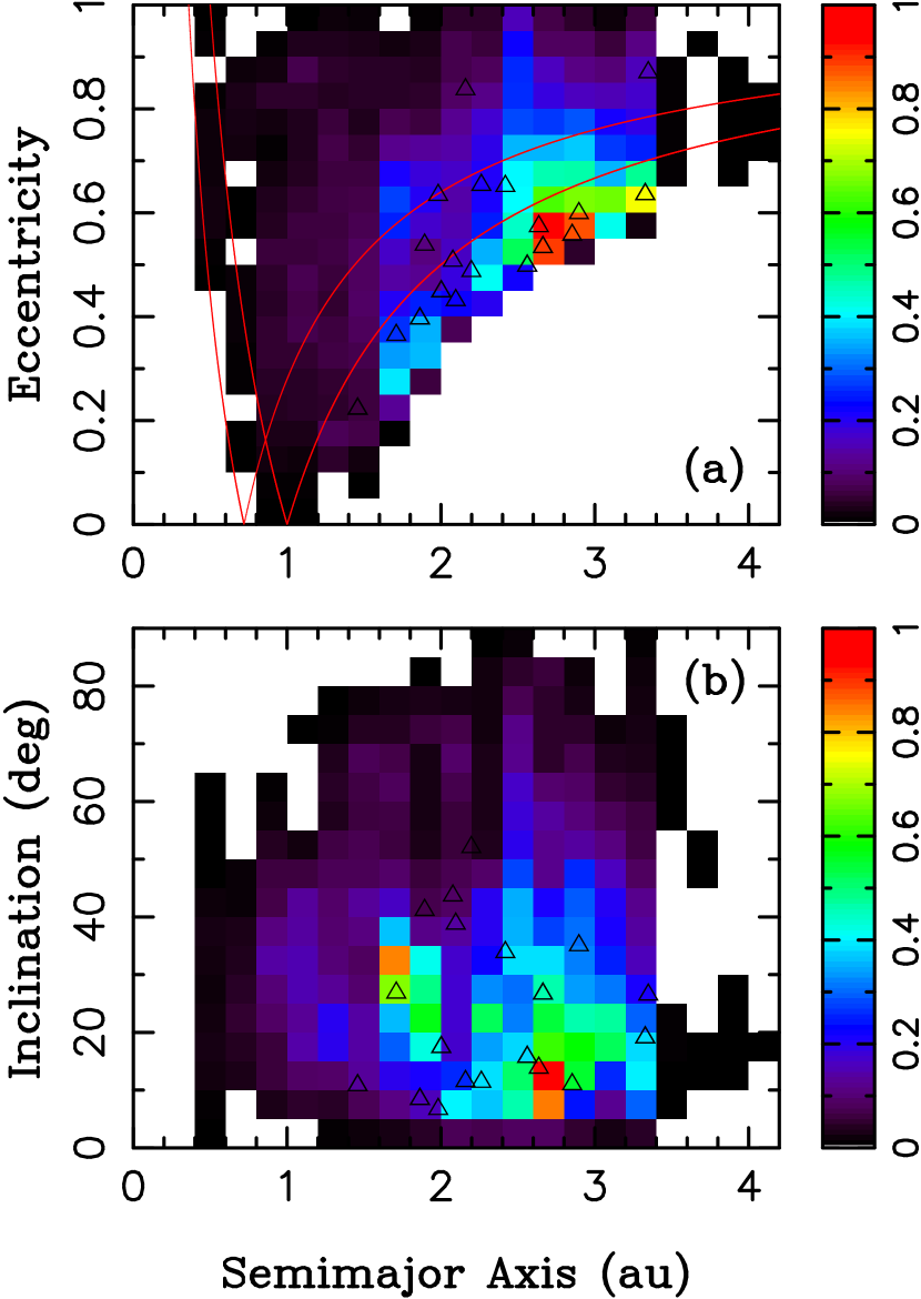
Figure 3: The orbital distribution of $D>10$ km NEAs obtained in our model. The color scale, which expresses the binned probability, appears on the right. The triangles show 22 known NEAs with $D>5$ km (data from WISE). We plot $D>5$ km NEAs here, because there are not enough $D>10$ km NEAs to make any sensible comparison between the model and observations. Also, our additional integrations with $D>5$ km asteroids show that they have similar dynamics to $D>10$ km asteroids and thus represent a useful reference.

We used our model results to determine the steady-state orbital distribution of large asteroids in NEA space. Figure 3 shows the distribution of $D>10$ km bodies in a plot where we computed the residence time of model NEAs on different orbits and binned them in $(a,e)$ and $(a,i)$ projections. Compared to Bottke et al. (2002), who presented similar plots applicable to smaller NEAs (mainly $D\sim 1$ km), our orbital distribution seems to be more concentrated at $2.5<a<3.0$ au with fewer NEA orbits below 2.5 au. This may correspond to the tendency of large NEAs to sample the inner and outer parts of the asteroid belt more equally than small NEAs (which predominantly start in the inner belt, roughly below 2.5 au).

The orbital distribution shown in Figure 3 does not have a very good statistics and more work will be needed to test things. It is also not clear whether the orbital distribution of large NEAs is consistent with the model expectation. This is because there are only two $D>10$ km NEAs to which our model strictly applies. As a proxy, we plotted in Figure 3 all known NEAs with $D>5$ km. Their orbital distribution appears to be similar to the model-derived distribution for $D>10$ km. Using $a=2.5$ au to split the NEA population into two parts, for example, we find that there should be roughly the same number of large NEAs with $a<2.5$ au and $a>2.5$ au. For comparison, there are 12 $D>5$ km NEAs with $a<2.5$ au and 10 with $a>2.5$ au.

4.3 Impact flux of $D>10$ km NEAs

The results of our numerical integrations were analyzed to resolve the motivating problem discussed in Section 2. From the number of impacts recorded by the Swift integrator and from the Öpik code we determined that $0.8\pm 0.3$ impacts of $D>10$ km asteroids are expected on the Earth in 1 Gyr. The estimated impact flux is thus well below the NEA-derived estimate of $\sim$7 $D>10$-km impacts per Gyr (Johnson et al. (2016), see also Chapman & Morrison (1994), Stuart & Binzel (2004), Le Feuvre & Wieczorek (2011) and Harris & D’Abramov (2015)). This confirms our expectations from Minton & Malhotra (2010) and Nesvorný et al. (2017). It shows that it is difficult to correctly estimate the steady-state impact flux of large asteroids from NEAs, because there are only a few large asteroids in NEA space at the present time, and because the collision probability of small NEAs cannot be extrapolated to large sizes.

Specifically, Johnson et al. (2016) assumed that there are 5 NEAs with $D>10$ km, including (1627) Ivar and (4954) Eric, which in fact are just over 8 km according to WISE. (3552) Don Quixote is probably a nearly extinct comet on a wide orbit and has a low terrestrial impact probability. This brings the number of relevant NEAs down to two (Ganymed and Eros).

In addition, if we interpret things correctly, the long term average of the number of $D>10$ km NEAs is $1.1\pm 0.5$ with the present population being a slight fluctuation above the average. Moreover, Johnson et al. (2016) applied the mean collisional probability with the Earth of $1.5\times 10^{-3}$ Myr^-1 for each NEA (e.g., Stuart 2001). This is appropriate for small NEAs, from which this estimate was derived, but not for large NEAs. We calculate that the mean collisional probability for each NEA with $D>10$ km is only $\simeq 7\times 10^{-4}$ Myr^-1, i.e. about two times lower. This happens because the outer part of the main belt is an important source of large NEAs (with about a half of their population deriving from $>2.9$ au). These outer belt asteroids have low terrestrial impact probability and weight down the mean.

In total, in the Gyr-long simulation with 15 clones, there were 38 impacts recorded on the terrestrial worlds (17 on Venus, 13 on Earth, and 8 on Mars; here we put together all our simulations for $D>10$ km to improve statistics). About 70% of the impactors started with $a<2.5$ au. This shows that the inner belt is the dominant source of impactors. The remaining impactors started with $2.5<a<2.8$ au (i.e. between the 3:1 and 5:2 resonances). None of the impacting particles had $a>2.8$ au initially, which demonstrates that the contribution of the main belt with $a>2.8$ au to the terrestrial impacts is relatively small. With the Öpik code we find that 70% of all terrestrial impactors started with $a<2.5$ au and 30% of impactors started with $2.5<a<2.8$ au. The Flora family is identified as the most important individual source of large impactors ($\simeq$10% of the total recorded impacts).

As for impacts on different target worlds, we found from the Öpik code that 0.84, 0.82, 0.42 and 0.044 $D>10$ km impacts are expected over 1 Gyr on Venus, Earth, Mars and the Moon, respectively. The impact rates derived from recorded impacts is similar (1.1, 0.9 and 0.5 impacts on Venus, Earth, Mars). Venus and Earth thus see comparable impact fluxes of large asteroids. Mars and the Moon receive roughly 1/2 and 1/20 of the number of Earth impactors, which is consistent with the previous work (e.g. Nesvorný et al. 2017). We found that the impact flux of $D>10$ km asteroids does not depend much on the assumed Yarkovsky drift; the population of clones with zero, negative and positive Yarkovsky drift rates all give the average number of 0.6-1 impacts on the Earth in 1 Gyr.

5 Conclusions

Existing estimates of the current flux of planetary impactors in the inner Solar System vary by a factor of $\sim$10 in different publications. For example, it has been suggested from the analysis of NEAs that $\simeq$7 impacts of diameter $D>10$ km bodies should have occurred on the Earth in the last 1 Gyr (e.g., Chapman & Morrison 1994, Stuart & Binzel 2004, Le Feuvre & Wieczorek 2011, Harris & D’Abramov 2015, Johnson et al. 2016). The impact rates inferred from models of NEA delivery from the main belt are at $\sim$7-14 times lower (e.g., Minton & Malhotra 2010, Nesvorný et al. 2017). Here we show that this problem is caused, in part, by the extrapolation of the impact flux from small ($D\sim 1$ km) to large sizes ($D>10$ km), where it is commonly assumed that the orbital distributions of small and large NEAs are the same.

In reality, they are not the same because small and large NEAs reach their orbits by different dynamical pathways. To demonstrate this, we conducted dynamical simulations of $D>10$ km main-belt asteroids as they evolve onto NEA orbits by radiation forces and resonances. We found that the current impact flux of $D>10$ km asteroids on the Earth is $0.8\pm 0.3$ Gyr^-1. The average impact probability of a $D>10$-km NEA is $\simeq$2 times lower than that of a $D\sim 1$-km NEA. Additional differences arise because: (1) most NEA-based studies used the absolute magnitudes to estimate that there are 5 $D>10$ km NEAs, while they are only two (Ganymed and Eros; or 3 if Don Quixote is counted), and (2) because the current number of two $D>10$ km NEAs may be a slight fluctuation above the long term average of $1.1\pm 0.5$.

Our work has important implications for our understanding of large impacts in the inner Solar System. For example, the K/T extinction event at 65 Ma is thought to have been caused by an impact of $D\sim 10$ km asteroid (Alvarez et al. 1980). Here we estimate that the average interval between terrestrial impacts of $D>10$ km asteroids is 1.2 Gyr. Having a $D\sim 10$ km asteroid hitting the Earth just 65 Ma may thus be somewhat special. Alternatively, the impactor could have been smaller. We may have also missed in our modeling some important dynamical mechanism that facilitates escape of large asteroids from the main belt. More complete models will need to be developed to help to disperse these doubts.

Figure 2: The model probability of having a specific number of $D>10$ km asteroids in NEA space at the present epoch (asterisks and solid line). The dashed line shows the best fit Poisson distribution with the 0.95 occurence rate.

References

- Alvarez et al. (1980) Alvarez, L. W., Alvarez, W., Asaro, F., & Michel, H. V. 1980, Science, 208, 1095
- Bottke & Greenberg (1993) Bottke, W. F., & Greenberg, R. 1993, Geophys. Res. Lett., 20, 879
- Bottke et al. (2002) Bottke, W. F., Morbidelli, A., Jedicke, R., et al. 2002, Icarus, 156, 399
- Bottke et al. (2005) Bottke, W. F., Durda, D. D., Nesvorný, D., et al. 2005, Icarus, 179, 63
- Bottke et al. (2006) Bottke, W. F., Jr., Vokrouhlický, D., Rubincam, D. P., & Nesvorný, D. 2006, Annual Review of Earth and Planetary Sciences, 34, 157
- Bottke et al. (2012) Bottke, W. F., Vokrouhlický, D., Minton, D., et al. 2012, Nature, 485, 78
- Bottke et al. (2015) Bottke, W. F., Vokrouhlický, D., Walsh, K. J., et al. 2015, Icarus, 247, 191
- Chapman (1994) Chapman, C. R., & Morrison, D. 1994, Nature, 367, 33
- Culler et al. (2000) Culler, T. S., Becker, T. A., Muller, R. A., & Renne, P. R. 2000, Science, 287, 1785
- Farinella & Vokrouhlicky (1999) Farinella, P., & Vokrouhlický, D. 1999, Science, 283, 1507
- Gladman et al. (1997) Gladman, B. J., Migliorini, F., Morbidelli, A., et al. 1997, Science, 277, 197
- Gomes et al. (2005) Gomes, R., Levison, H. F., Tsiganis, K., & Morbidelli, A. 2005, Nature, 435, 466
- Granvik et al. (2016) Granvik, M., Morbidelli, A., Jedicke, R., et al. 2016, Nature, 530, 303
- Granvik et al. (2017) Granvik, M., Morbidelli, A., Vokrouhlický, D., et al. 2017, A&A, 598, A52
- Greenberg (1982) Greenberg, R. 1982, AJ, 87, 184
- Greenstreet et al. (2012) Greenstreet, S., Ngo, H., & Gladman, B. 2012, Icarus, 217, 355
- Hanuš et al. (2011) Hanuš, J., Ďurech, J., Brož, M., et al. 2011, A&A, 530, A134
- Harris & D’Abramo (2015) Harris, A. W., & D’Abramo, G. 2015, Icarus, 257, 302
- Hartmann & Neukum (2001) Hartmann, W. K., & Neukum, G. 2001, Space Sci. Rev., 96, 165
- Holsapple (1993) Holsapple, K. A. 1993, Annual Review of Earth and Planetary Sciences, 21, 333
- Johnson et al. (2016) Johnson, B. C., Collins, G. S., Minton, D. A., et al. 2016, Icarus, 271, 350
- Le Feuvre & Wieczorek (2011) Le Feuvre, M., & Wieczorek, M. A. 2011, Icarus, 214, 1
- Levison & Duncan (1994) Levison, H. F., & Duncan, M. J. 1994, Icarus, 108, 18
- Levison & Duncan (1994) Mazrouei, S., Ghent, R. R., Bottke, W. F., & Parker, A. H. 2017, Science, submitted
- Mainzer et al. (2011) Mainzer, A., Bauer, J., Grav, T., et al. 2011, ApJ, 731, 53
- Migliorini et al. (1998) Migliorini, F., Michel, P., Morbidelli, A., Nesvorny, D., & Zappala, V. 1998, Science, 281, 2022
- Minton & Malhotra (2010) Minton, D. A., & Malhotra, R. 2010, Icarus, 207, 744
- Morbidelli & Nesvorný (1999) Morbidelli, A., & Nesvorný, D. 1999, Icarus, 139, 295
- Neukum et al. (2001) Neukum, G., Ivanov, B. A., & Hartmann, W. K. 2001, Space Sci. Rev., 96, 55
- Nesvorný et al. (2002) Nesvorný, D., Morbidelli, A., Vokrouhlický, D., Bottke, W. F., & Brož, M. 2002, Icarus, 157, 155
- Nesvorný et al. (2007) Nesvorný, D., Vokrouhlický, D., Bottke, W. F., Gladman, B., & Häggström, T. 2007, Icarus, 188, 400
- Nesvorný et al. (2017) Nesvorný, D., Roig, F., & Bottke, W. F. 2017, AJ, 153, 103
- Robbins (2014) Robbins, S. J. 2014, Earth and Planetary Science Letters, 403, 188
- Statler (2009) Statler, T. S. 2009, Icarus, 202, 502
- Strom et al. (2005) Strom, R. G., Malhotra, R., Ito, T., Yoshida, F., & Kring, D. A. 2005, Science, 309, 1847
- Stuart & Binzel (2004) Stuart, J. S., & Binzel, R. P. 2004, Icarus, 170, 295
- Valsecchi & Gronchi (2011) Valsecchi, G. B., & Gronchi, G. F. 2011, EPSC-DPS Joint Meeting 2011, 402
- Valsecchi & Gronchi (2015) Valsecchi, G. B., & Gronchi, G. F. 2015, Highlights of Astronomy, 16, 492
- Vokrouhlický et al. (2003) Vokrouhlický, D., Nesvorný, D., & Bottke, W. F. 2003, Nature, 425, 147
- Vokrouhlický et al. (2012) Vokrouhlický, D., Pokorný, P., & Nesvorný, D. 2012, Icarus, 219, 150
- Vokrouhlický et al. (2015) Vokrouhlický, D., Bottke, W. F., Chesley, S. R., Scheeres, D. J., & Statler, T. S. 2015, Asteroids IV, 509
- Wisdom & Holman (1991) Wisdom, J., & Holman, M. 1991, AJ, 102, 1528