Scale invariant jets: from blazars to microquasars

Scale invariant jets: from blazars to microquasars

Abstract

Black holes, anywhere in the stellar-mass to supermassive range, are often associated with relativistic jets. Models suggest that jet production may be a universal process common in all black hole systems regardless of their mass. Although in many cases observations support such hypotheses for microquasars and Seyfert galaxies, little is known on whether boosted blazar jets also comply with such universal scaling laws. We use uniquely rich multiwavelength radio light curves from the F-GAMMA program and the most accurate Doppler factors available to date to probe blazar jets in their emission rest frame with unprecedented accuracy. We identify for the first time a strong correlation between the blazar intrinsic broad-band radio luminosity and black hole mass, which extends over $\sim$ 9 orders of magnitude down to microquasars scales. Our results reveal the presence of a universal scaling law that bridges the observing and emission rest frames in beamed sources and allows us to effectively constrain jet models. They consequently provide an independent method for estimating the Doppler factor, and for predicting expected radio luminosities of boosted jets operating in systems of intermediate or tens-of-solar mass black holes, immediately applicable to cases as those recently observed by LIGO.

1 Introduction

Blazars constitute unique laboratories to study extreme astrophysics, from relativistic magnetohydrodynamics and shocks, to particle acceleration, ultra-high energy cosmic rays and neutrino production. They are divided into two sub-classes: Flat Spectrum Radio Quasars (FSRQs) and BL Lac objects (BL Lacs) and are most famous for their extreme variability, apparent superluminal motion and $\gamma$-ray loudness since they comprise the largest detected population of the Fermi $\gamma$-ray observatory (Acero et al., 2015). Understanding the relativistic highly collimated plasma outflows of blazar jets has proven extremely difficult due to the relativistic effects dominating their emission from radio to $\gamma$-rays (Blandford & Königl, 1979). These relativistic effects are quantified by the Doppler factor $\delta=[\gamma(1-\beta\cos\theta)]^{-1}$, where $\gamma$ is the Lorentz factor ($\gamma=(\sqrt{1-\beta^{2}})^{-1}$), $\beta$ is the velocity of the jet in units of speed of light, and $\theta$ is the angle between their jet axis and the observer’s line of sight. Even a small spread in the values of $\gamma$ and $\theta$ among blazars results in a large spread in observed properties, severely complicating the search for empirical correlations that can confirm or constrain jet models. If $\delta$ could be confidently estimated, however, these relativistic effects could be corrected for and blazar jets could be studied in their emission rest frame.

Several methods have been proposed for estimating blazar Doppler factors, but they frequently yield discrepant results (Liodakis et al., 2017b). Given the numerous assumptions entering each method, it is often challenging to identify the most accurate estimate for any given blazar. Two recent breakthroughs have, however, made such a task tractable for the first time. First, through population modeling of unbiased blazar samples (Liodakis & Pavlidou, 2015a), Doppler factor estimates based on variability studies and the assumption of equipartition between synchrotron emitting particles and magnetic field (Readhead, 1994; Lähteenmäki & Valtaoja, 1999; Hovatta et al., 2009) were shown to be the most accurate (Liodakis & Pavlidou, 2015b). Second, multi-frequency F-GAMMA radio data have recently enabled the calculation of the highest-ever accuracy variability Doppler factors for 58 well-studied blazars (Liodakis et al., 2017a).

Correlations between the BH mass ($M_{\rm BH}$) and monochromatic radio flux density, or the monochromatic radio flux density and the X-ray flux density or even all the above combined, have long been established (e.g. Merloni et al., 2003). The latter suggests the existence of a plane, termed “fundamental plane of black hole activity”, which extends from X-ray binaries to active galaxies. These results support the hypothesis of scale invariance, which implies that the jet formation processes are independent of the black hole mass of the system. Such a hypothesis has been predicted by theoretical models (Heinz & Sunyaev, 2003).

Merloni et al. (2003) as well as similar attempts to establish a relation connecting BH-powered jets of different $M_{\rm BH}$ (Nagar et al., 2002; Falcke et al., 2004; Körding et al., 2006; Plotkin et al., 2012; Saikia et al., 2015) have either explicitly avoided blazars focusing on low-luminosity active galactic nuclei (LLAGNs) or have included a handful of blazars. In the latter case they have either ignored the relativistic effects or specifically chosen their sample to include only low-beamed sources. In cases were there was some treatment of the relativistic effects (Falcke et al., 2004; Körding et al., 2006; Plotkin et al., 2012), the common practice was to use a single value of $\delta$, when in reality Doppler factors are estimated to range between 1 and 45 based on individual source studies (Lähteenmäki & Valtaoja, 1999; Hovatta et al., 2009; Fan et al., 2009; Liodakis et al., 2017a) and between 1 and 60 based on population studies (Liodakis & Pavlidou, 2015a).

However, studies focused on blazars, fully and accurately accounting for their relativistic effects cannot be circumvented, specially if the aim is to study the physics of jets: it is only in such highly beamed sources where we are certain that the observed spectrum is dominated by the jet emission. For this reason, the extension of such scalings to blazars should have a strong impact on unification models of radio-loud active galactic nuclei and our knowledge of BH-powered jets, increasing manyfold our ability to constrain jet models.

There have been attempts to create similar scaling relations in blazars either using luminosity-luminosity correlations (Nemmen et al., 2012; Fan et al., 2017) or different jet quantities with the properties of the central engine (Wang et al., 2004; Hovatta et al., 2010; Bower et al., 2015). However, the relativistic effects hamper any attempt to establish a strong correlation between the rest-frame emission of the jet and the $M_{\rm BH}$ in beamed sources.

Even if we account for the relativistic effects properly, blazars are known to show extreme variability across all frequencies. Therefore, the use of single-epoch measurements of flux densities as a proxy of the source luminosity is highly problematic. In addition, many different mechanisms (e.g. hot corona, synchrotron radiation, and synchrotron self-Compton) contribute to the blazar X-ray flux. Disentangling the different contributions has been so far extremely uncertain at best, making the use of the black hole fundamental plane or similar relations unfeasible.

In this work, in order to overcome all such limitations and probe the physics of blazars we propose a new method to explore the connection between jet power and supermassive black hole in beamed sources by using the rest-frame broad-band radio luminosity ($\mathcal{L}_{\rm int}^{\rm Br-B}$) and the $M_{\rm BH}$.

This work is organized as follows: In section 2 we present the data used in this work, and the manner of their analysis. In section 3 we present the correlation analysis and the best-fit relation. In section 4 we discuss our findings and in section 5 we summarize our results and conclusions.

Throughout this work the adopted cosmology is $H_{0}=71$ ${\rm km\,s^{-1}\,Mpc^{-1}}$, $\Omega_{m}=0.27$ and $\Omega_{\Lambda}=1-\Omega_{m}$ (Komatsu et al., 2009).

2 Data & Analysis

Our sample is a sub-set of the sources monitored by the F-GAMMA program including all sources with both an available Doppler factor and $M_{\rm BH}$ estimates. The F-GAMMA program monitored a total of about 100 blazars detected by Fermi for eight years with roughly monthly cadence at ten frequencies from 2.64 to 142.33 GHz (Fuhrmann et al., 2016). The Doppler factors are taken from (Liodakis et al., 2017a). In Liodakis et al. (2017a), a novel approach is used to model and track the evolution of the flares through multiple frequencies. That method has provided the most accurate variability Doppler factor estimates to date with an on average 16% error. We use only estimates with quality indicator “confident” or “very confident” to ensure robust results. The level of confidence is defined by the number of available frequencies and flares used in the estimation of the Doppler factor (see Liodakis et al., 2017a). The number of sources in our sample is 26 (20 FSRQs, 4 BL Lacs, and 2 radio galaxies). In order to extend our sample towards lower black hole masses, we also included three $\gamma$-ray loud Narrow Line Seyfert 1 galaxies (NLS1s, Angelakis et al., 2015) for which there was a Doppler factor computed with the same method as in Liodakis et al. (2017a). In total our sample consists of 29 sources with $M_{\rm BH}$ spanning from $\sim 10^{6.5}$ to $10^{9.5}$ $M_{\odot}$.

2.1 Intrinsic broad-band radio luminosity

We calculated the intrinsic broad-band radio luminosity ($\mathcal{L}_{\rm int}^{\rm Br-B}$) of our sources using data from the F-GAMMA program. For each frequency we use the maximum likelihood approach described in Richards et al. (2011) to calculate the maximum likelihood mean flux-density taking into account errors in measurements, uneven sampling and source variability. From that we construct the “mean” spectrum which we convert to the intrinsic luminosity using the Doppler factor estimates from Liodakis et al. (2017a). Accounting for the relativistic effects in estimating the rest-frame broad-band radio luminosity in blazars is crucial in order to identify the correct correlation (see section 4).

We convert the maximum likelihood mean flux density for each frequency to the intrinsic luminosity using the following equation:

$$S_{\nu}=\frac{L_{\nu}\delta^{p}}{4\pi{d_{L}^{2}}}(1+z)^{1+s},$$ (1)

where $S_{\nu}$ is the flux-density at a given frequency $\nu$, $L_{\nu}$ the intrinsic luminosity at that frequency, $\delta$ is the Doppler factor, $d_{L}$ the luminosity distance, $z$ the redshift, $s$ the spectral index which we have defined as $S\propto\nu^{s}$, and $p$ is equal to $p=2-s$ for the continuous, and $p=3-s$ for the discrete jet case.

By integrating over frequency we calculate the $\mathcal{L}_{\rm int}^{\rm Br-B}$ for each source assuming either a continuous jet ($\mathcal{L}_{\rm int,c}^{Br-B}$) or a discrete jet ($\mathcal{L}_{\rm int,d}^{\rm Br-B}$). We estimate the uncertainty of the $\mathcal{L}_{\rm int}^{\rm Br-B}$ through formal error propagation taking into account errors in the Doppler factor (Liodakis et al., 2017a), flux-density, spectral index, and redshift. For the error in the Doppler factor estimates for the three NLS1s we assumed the 16% average error from Liodakis et al. (2017a). Since our redshift estimates are all spectroscopic we have assumed a common error of $\delta z$=0.01 .

2.2 BH mass estimation

In order to estimate the $M_{\rm BH}$ of our sample we used data from Torrealba et al. (2012) and the scaling relations from Shaw et al. (2012) using the line luminosities of the MgII and Hb spectral lines. The scalings were calibrated using the virial mass estimation method. The uncertainty of the $M_{\rm BH}$ for each source was the result of error propagation. We complemented our sample with values (and their error) from the literature with estimates using the same method for consistency (Yuan et al., 2008; Shaw et al., 2012; Zamaninasab et al., 2014, and references therein). When there was no error estimate for a literature value (Yuan et al., 2008; Zamaninasab et al., 2014, see Table 2), we assumed as error the average uncertainty of the available estimates using the same spectral line. We avoided using methods that involve assumptions on the radio flux density, beaming, Spectral Energy Distribution (SED) fitting etc., that could potentially create artificial correlations. All the estimates for the $\mathcal{L}_{\rm int}^{\rm Br-B}$ and $M_{\rm BH}$ used in this work are summarized in Table 2.

3 Correlation and best-fit model

Assuming that the jet is composed of a series of plasma blobs (discrete jet) we tested for a correlation between the $\mathcal{L}_{\rm int,d}^{\rm Br-B}$ and $M_{\rm BH}$. We used the partial correlation test (Akritas & Siebert, 1996) in order to obtain the Kendall correlation coefficient ($\tau$) and its significance taking into account the effects of redshift. The partial correlation test yielded a correlation coefficient of $\tau=0.35$ with $2\times 10^{-3}$ probability of uncorrelated samples, indicating a moderate correlation. If we assume the jet is a continuous stream of plasma (continuous jet, $\mathcal{L}_{\rm int,c}^{\rm Br-B}$), the correlation becomes significantly stronger ($\tau=0.51$ with $5\times 10^{-6}$ probability of no correlation). The correlation is stronger in this case, which is to be expected since the continuous jet is, most likely, the most accurate representation of the jet structure, as has been repeatedly supported by interferometric radio observations (VLBI, e.g. Zensus, 1997). For this reason, for the remaining of this work we focus on the continuous jet case. Examining different subsamples there was no case were the p-value was $>10^{-3}$ supporting the robustness of the correlation. For FSRQs alone we find $\tau=0.44$ with p-value $6\times 10^{-4}$. Including the BL Lacs the test yielded $\tau$=0.43 with p-value $7\times 10^{-4}$, and including the radio galaxies $\tau$=0.45 with probability $2\times 10^{-4}$. The significant correlation found in all cases strongly suggests that this is a real trend and not an artifact of the large range of $M_{\rm BH}$.

Having established that a significant correlation exists, we performed a fit between $\mathcal{L}_{\rm int,c}^{\rm Br-B}$ and $M_{\rm BH}$ in log-space. Assuming a linear model of the form $\log\mathcal{L}_{\rm int,c}^{\rm Br-B}=A\times\log(\frac{M}{10^{8}M_{\odot}})+B$. The fit was performed using the BCES bisector methods described in Akritas & Bershady (1996) which takes into account errors in both axis as well as intrinsic scatter. The best-fit line between the $\mathcal{L}_{\rm int,c}^{\rm Br-B}$ and the $M_{\rm BH}$ would then be,

$$\log\left(\frac{\mathcal{L}_{\rm int,c}^{\rm Br-B}}{Watt}\right) = (1.12\pm{0.13})\times\log(\frac{M}{10^{8}M_{\odot}})+(35.5\pm{0.1}).$$

The $\log\mathcal{L}_{\rm int,c}^{\rm Br-B}$ versus $\log M_{\rm BH}$ plot is shown in Fig. 1 together with the best-fit line. The best-fit results do not depend on the adopted linear best-fit method. For example, if we consider only intrinsic scatter using the bisector method of Isobe et al. (1990), the best-fit the slope and intercept become $A=1.05\pm 0.01$ and $B=35.55\pm 0.04$. In fact, for any of the methods described in Akritas & Bershady (1996) and Isobe et al. (1990) the results remain consistent, within the uncertainties.

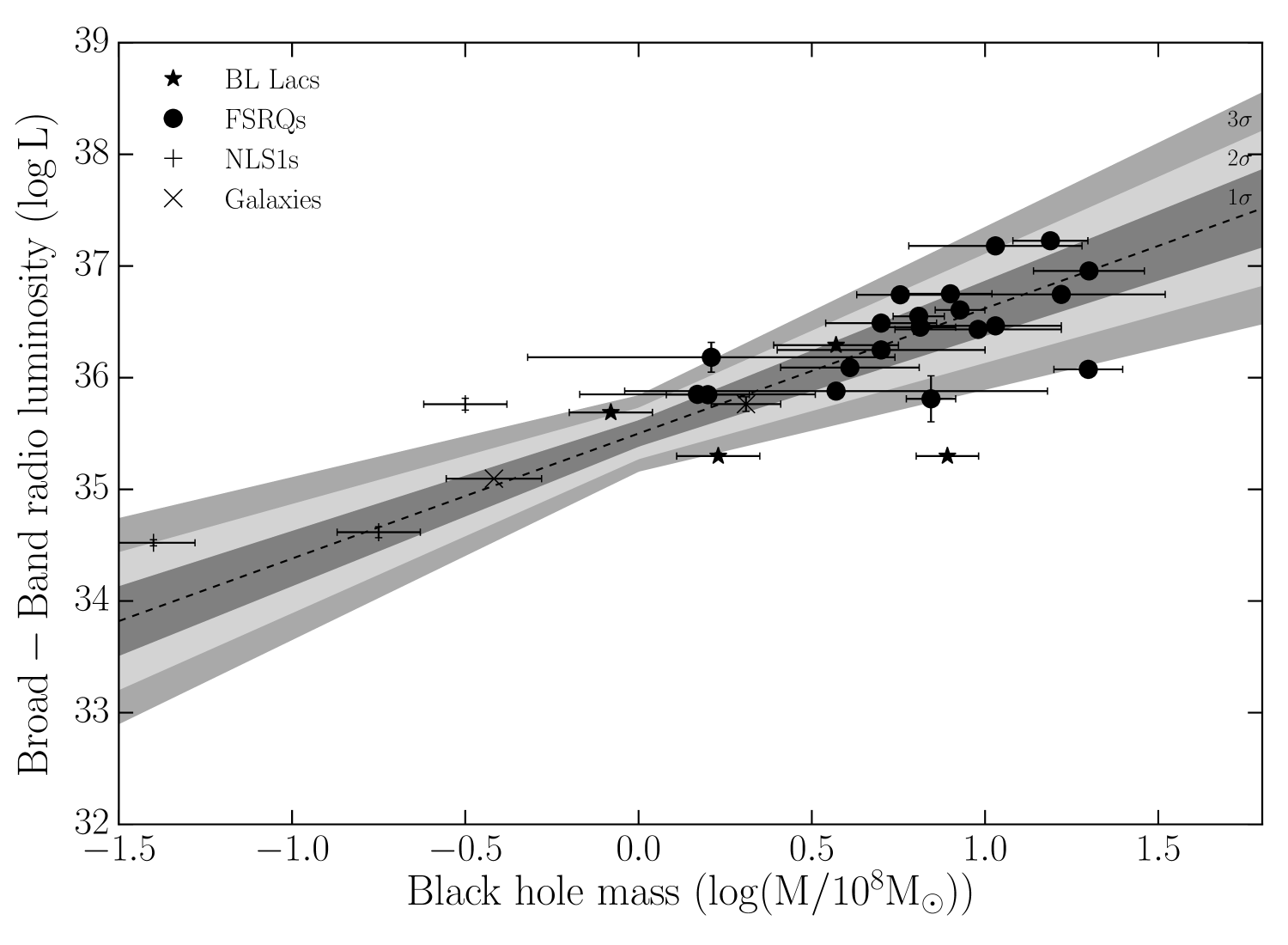
Figure 1: Intrinsic broad-band radio luminosity ($\mathcal{L}_{\rm int,c}^{\rm Br-B}$) versus $M_{\rm BH}$ (luminosity is in Watts). The dashed line represents the best-fit relation. The grey shaded areas are the 1$\sigma$, 2$\sigma$, and 3$\sigma$ confidence regions respectively, taking into account the error on both slope and intercept.

There is some scatter around the best-fit relation which if intrinsic has been taken into account during the fit. To examine whether this scatter is induced by the errors in the measurements or it is intrinsic, we compare the average distance of each measurement from the best-fit relation to the average distance due to the uncertainty. Using the best-fit line, for each measurement of $M_{\rm BH}$ we estimated the predicted intrinsic radio broad-band luminosity and subtracted it from the observed one to determine the distance in the y-axis. We perform the reverse for the x-axis. We calculate the vertical distance for each observation using $z=\sqrt{x^{2}+y^{2}}$ and the scatter is estimated as $\rm Sc=\sqrt{(\sum_{i=1}^{N}z_{i}^{2})/N}$. For the expected distance due to error we use the average error on the y- and x-axis and calculate the vertical distance and scatter in the same manner. We found that the scatter of our sample is $\rm Sc=0.56$ whereas the scatter due to error is $\rm Sc_{error}=0.19$ suggesting that the scatter around the best-fit scaling is intrinsic.

Previous studies have opted to use the monochromatic radio luminosity of the jet (Nagar et al., 2002; Merloni et al., 2003). We can estimate the mean radio luminosity at a fixed frequency and account for the blazar variability using maximum likelihood. However, observer’s frame frequencies are significantly different in the emission rest-frame due to the large redshift span ($z=[0,2]$) of our sample. Since different rest-frame frequencies probe different emission regimes (optically thick or optically thin) in different blazars as well as different regions, the use of single frequency measurements should affect the scatter of the correlation (see also discussion in Falcke et al., 2004). Figure 2 shows the intrinsic monochromatic luminosity at 4.8 GHz versus $M_{\rm BH}$ for our sample. There is a strong correlation ($\tau=0.44$, p-value $2\times 10^{-4}$) and a slope of $A=0.83\pm 0.17$ and $B=24.8\pm 0.15$. Although we find consistent results between monochromatic and broad-band luminosities, there is a larger scatter ($\rm Sc=0.70$) around the best-fit line in the former case. We therefore conclude that using the broad-band luminosity provides stronger constrains for the $\mathcal{L}_{\rm int}$-$M_{\rm BH}$ relation.

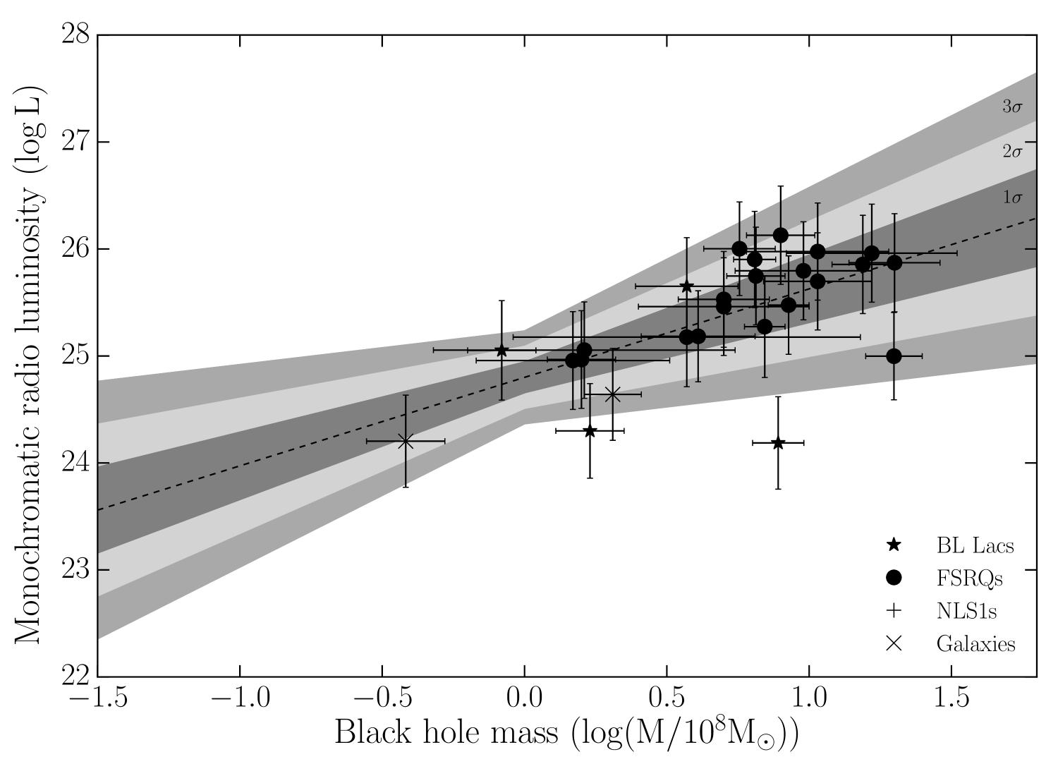
Figure 2: Intrinsic monochromatic radio luminosity (4.8 GHz) versus $M_{\rm BH}$. The dashed line indicates the best-fit model. Symbols and grey areas as in Fig. 1.

If jets are indeed scale invariant, then stellar mass BH systems (i.e. microquasars) will have intrinsic broad-band radio luminosities of $\sim 10^{27}-10^{28}$ Watt according to the best-fit relation derived above. To test this prediction, we collected archival data from the literature for five well studied microquasars with available contemporaneous multi-wavelength radio observations. Given the uncertainty in the measurements of different parameters for the microquasars (viewing angle, jet velocity, distance, $M_{\rm BH}$), with each source having multiple estimates in the literature, we used a Monte-Carlo approach to calculate the mean and spread (minimum to maximum) of the $\mathcal{L}_{\rm int,c}^{\rm Br-B}$ and $M_{\rm BH}$ for each source (see Appendix A).

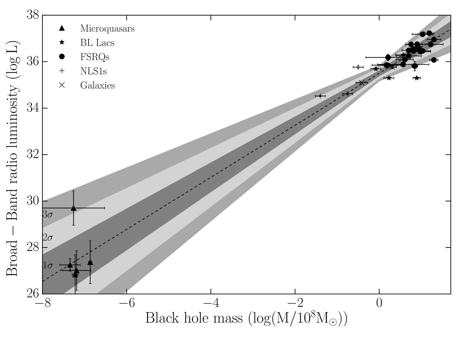
Figure 3: Intrinsic broad-band radio luminosity ($\mathcal{L}_{\rm int,c}^{\rm Br-B}$) versus $M_{\rm BH}$. Luminosity is in Watts, and $M_{\rm BH}$ in $\rm 10^{8}M_{\odot}$. The dashed line represents the best-fit relation using only sources with a supermassive BH. Symbols and grey areas as in Fig. 1. For the microquasars every point represents the mean and the errorbar the spread given the different estimates for each source.

Figure 3 shows the position of the microquasars with respect to the best-fit line derived from the supermassive $M_{\rm BH}$ sample. The values represent the mean and the errorbars the spread given the different estimates for each source. All microquasars are consistent with the best-fit $\mathcal{L}_{\rm int,c}^{\rm Br-B}-M_{\rm BH}$ relation for blazars, within the 3$\sigma$ confidence area of the fit, straddling the best-fit line. In fact, four out of the five sources are within 1$\sigma$. While uncertainties of both fit and measurements are quite significant at this mass range, our results suggest that the scaling derived from the blazar sample is in fact a universal scaling extending over at least $\sim$9 orders of magnitude both in $\mathcal{L}_{\rm int,c}^{\rm Br-B}$ and $M_{\rm BH}$.

4 Discussion

Taking into account the relativistic effects is essential in order to identify the correct scaling. We investigated the $\mathcal{L}^{\rm Br-B}-M_{\rm BH}$ relation obtained after only correcting for redshift. A correlation is detected, however, the sources appear to occupy unrelated regions of the $\mathcal{L}^{\rm Br-B}-M_{\rm BH}$ plot (Fig. 4 upper panel). The slope is much steeper (A=2.45$\pm$0.22) with larger scatter. Most importantly the scaling from the supermassive BHs under-predicts the broad-band radio luminosity of microquasars by roughly ten orders of magnitude. Accounting for beaming not only brings all classes with supermassive BHs onto one single line, but it also accurately predicts the position of their stellar mass BH counterparts.

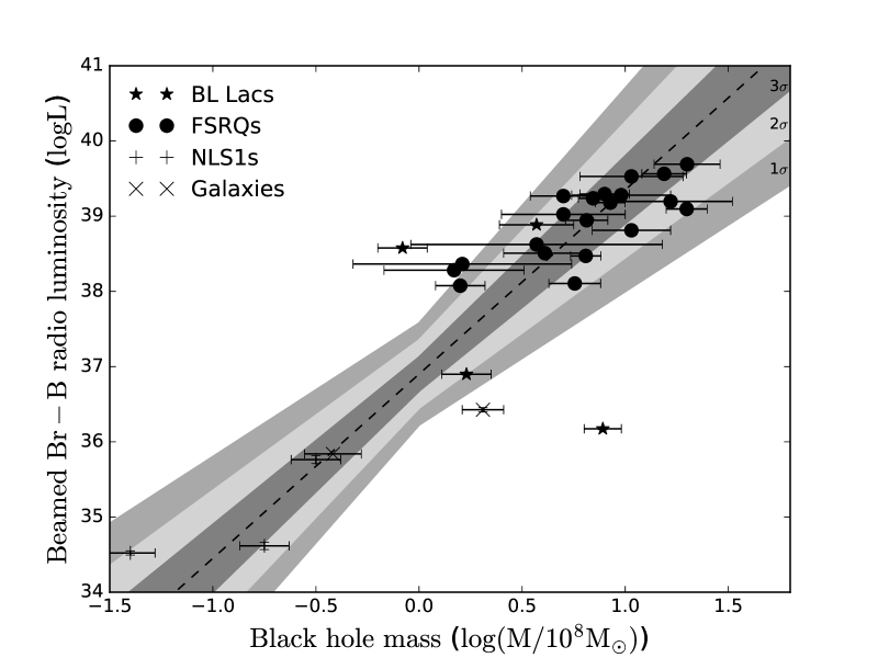
Figure 4: Observer-frame broad-band radio luminosity versus $M_{\rm BH}$. The dashed line indicates the best-fit model. Symbols and grey areas as in Fig. 1.

A non-linear relation between the flux of the jet (and hence the luminosity) and the $M_{\rm BH}$ ($S_{\nu}\propto M_{BH}^{1.42}$) was predicted by Heinz & Sunyaev (2003), for typical flat-spectrum core-dominated radio jets and standard accretion scenarios. They also commented that variations in the other source parameters, like the accretion rate (measured in Eddington units), the viscosity parameter and viewing angle will only cause a mass-independent scatter around this relation. This theoretical prediction between radio luminosity and black hole mass is not entirely consistent with the linear relation derived in this work (2.3$\sigma$ difference). However, Heinz & Sunyaev (2003) pointed that if the jets are powered by spin extraction from the black hole (Blandford & Znajek, 1977), then the jet variables will not only depend on $M_{\rm BH}$ and the accretion rate ( which was the working assumption in Heinz & Sunyaev, 2003) but on the spin as well. It is also discussed in Merloni et al. (2003) that the radio luminosity would be sensitive to the spin of the black hole in the case where the process of jet formation is dependent on the spin. Within the framework of the Blandford-Znajek mechanism (Blandford & Znajek, 1977), the luminosity of the jet should be proportional to $M_{\rm BH}$ : $L_{BZ}\propto\dot{m}f(a)^{2}M_{\rm BH}$ (Tchekhovskoy et al. (2010); Daly (2016) and references therein) where $\dot{m}$ is the accretion rate in Eddington units and $f(a)$ is the spin function ($f(a)=a/[1+\sqrt{1-a^{2}}]$, $a$ being the dimensionless spin parameter). A linear scaling such as the one we find is then expected provided that the product $\dot{m}f(a)^{2}$ does not vary significant between sources and does not depend on $M_{\rm BH}$.

The intrinsic scatter around the best-fit relation may be due to either $\dot{m}$ or $f(a)$ random variations around the blazar mean $\dot{m}f(a)^{2}$ product. An additional source of scatter could be variations of the broad-band luminosity. Our estimates of the $\mathcal{L}^{\rm Br-B}$ are limited by the time span of the observations. Although the 8 year dataset of the F-GAMMA program is sufficiently long, it is still possible that exceptional events can occur outside the monitoring period (so that the mean luminosity is actually higher) or alternately a source was unusually active (so that the mean luminosity is actually lower). Cases such as the ones described above are both unlikely and should have a relatively small contribution to the overall scatter.

Our best-fit slope is consistent with those of similar studies on LLAGNs and microquasars ($1.14\pm 0.16$, Nagar et al., 2002 and $1.23\pm 0.20$, Merloni et al., 2003) however with smaller scatter. The larger scatter found in LLANGs could be the result of mild beaming that has not been accounted for (see Merloni et al., 2003) or other effects related to the use of single-frequency measurements. Beaming effects can also be responsible for the slightly steeper slope in Merloni et al. (2003), since the sources whose beaming is important (blazar-like sources) will have systematically higher luminosities compared to the parent population. Thus the slope will be swifted to stepper values. The fact that our results are consistent with those derived for unbeamed sources: (a) provides further support that we are efficiently correcting for the relativistic effects; and (b) provides supportive evidence for the universality of the derived scaling.

The microquasars that agree best with the relation derived from blazars all share the same accretion state while the one at 3$\sigma$ is in the intermediate-soft state (see Appendix A). This would suggest that the blazars in our sample are in a similar accretion state as the ones that lie on the best-fit line i.e the hard state. The presence of a big blue bump (BBB) in the SED of FSRQs could indicate a geometrically thin, optically thick disk, contrary to the disk of microquasars in the hard state (e.g., Done et al., 2007). Although the optical emission from the boosted-jet can dominate over that of the accretion disc and conceal such features in the SED, out of the 20 FSRQs in our sample only 3 sources have a visible BBB. We have verified that excluding these sources from our analysis has no effect on the derived best-fit relation (B remains the same, A=$1.14\pm 0.14$). Same accretion states would also suggest that the Eddington ratios ($R_{Edd}=L_{bol}$/$L_{Edd}$) of the supermassive BH sample would be similar with those of the hard-state microquasars. Although estimates of $R_{Edd}$ are uncertain for beamed sources, recent studies suggest that $R_{Edd}$ maybe less than 10% in the majority of blazars and radio galaxies (Ghisellini et al., 2010; Chen et al., 2015; Xiong et al., 2015). Narrow Line Seyfert 1 are known to have a high $R_{Edd}$, however, recent studies suggest that $R_{Edd}<10$% in the $\gamma-$ray loud NLS1s as well (Liu et al., 2016). In order to estimate the Eddington ratio for the sources in our sample, we used the Kaspi et al. (2000) relation between Eddington ratio and monochromatic luminosity at 5100 Å, and we estimated $R_{Edd}$ in nine of them. Although it is not clear whether such relations, which have been established for radio-quiet objects, are also applicable to radio-loud quasars, we found that eight out of them may have $R_{Edd}<1$%, which is almost identical to the Eddington ratios of the microquasars when in their hard state. The only source with $R_{Edd}>1$% is one of the three sources with a visible BBB in their SED. Although the lack of $R_{Edd}$ estimates prevents us from drawing strong conclusions, it would appear that, on average, the blazars in our sample share the same accretion state with hard-state microquasars. It makes sense to compare blazars and microquasars since, after all, they both have jets. We find that $\mathcal{L}^{\rm Br-B}\propto M_{\rm BH}$, for all of them which is consistent with the predictions of Blandford and Znajek mechanism. So, if this is the case, and if the accretion regime is different in hard-state microquasars and some of the blazars in our sample (say powerful FSRQs) then our results suggest that the Blandford and Znajek mechanism can operate, irrespective of the accretion regime (e.g., McKinney, 2005; Tchekhovskoy et al., 2010). As discussed above, differences in $\dot{m}$ (i.e different accretion state) between sources would increase the scatter around the best-fit relation. It will then be interesting to populate our sample with FSRQs with visible and strong BBB, and sources with higher $R_{Edd}$, in order to examine if the best-fit model moves closer to the microquasar in the intermediate state and the overall scatter decreases. This would suggest that blazars also have two accretion regimes.

The scaling derived in this work provides for the first time an independent method of estimating the Doppler factor starting from first principles. Estimates of the BH mass and the observer’s frame broad-band radio luminosity can be used to derive Doppler factor estimates within the scatter of the best-fit relation. These Doppler factor estimates can be used to either reduce the number of free parameters of SED models or, alternately, used to distinguish between acceptable SED models. However, the scaling relation was derived using the mean observer’s frame $\mathcal{L}^{\rm Br-B}$ based on the F-GAMMA 8-year dataset. Given the possibility of changes in the Doppler factor during a significant event (bends in the jet, local acceleration e.g. Homan et al., 2009, 2015), deriving a Doppler factor from single-epoch observations might not yield a representative estimate for that particular event.

5 Summary & Conclusions

Using the multi-wavelength radio light curves of the F-GAMMA program and the most accurate Doppler factors available to date, we identified a strong linear correlation between the intrinsic broad-band radio luminosity of the jets and the black hole mass that extends 9 orders of magnitude to stellar mass black hole systems. Such a universal scaling law is the first ever to bridge observer’s and emission rest-frames in beamed sources.

The scaling derived in this work constitutes an important breakthrough in blazar physics. First, it comprises clear evidence of scale-invariant BH jets and of a connection between the properties of supermassive black holes and the large scale jets they cause in beamed sources. Second, it provides a solid prediction on the $\mathcal{L}_{\rm int,c}^{\rm Br-B}$ of intermediate mass black holes if such exist, and if they form jets. Third, it provides an independent method of estimating the Doppler factor, which will undoubtedly prove an important contribution in constraining SED fitting and the different jet emission models in beamed sources. Fourth, the universality of the scaling would suggest that blazars are in a similar accretion regime as the hard state in microquasars. Finally, our findings point towards the Blandford-Znajek mechanism as the dominant mechanism for jet production in black hole powered jets, and set strong constrains on other potential jet models since they have to reproduce such linear relation.

Appendix A Microquasars

Our sample of microquasars was selected on the availability of contemporaneous multi-wavelength radio observations. Their data were measured from compact synchrotron jets (hard state) for all sources except Cyg X-3 (the microquasar with the highest luminosity in Fig. 3) whose data were taken from ballistic ejecta during radio outbursts. Calculating $\mathcal{L}^{\rm Br-B}_{\rm int,c}$ for microquasars is not trivial, the main obstacle being the lack of robust estimates for key parameters (e.g., distance, Doppler factor), as well as the lack of contemporaneous multi-wavelength radio observations. In most cases the range of available frequencies was confined in the lower frequency range ($<$ 43 GHz). The observed flux density at higher frequencies was the result of extrapolation by assuming that the spectral index derived from the highest available frequencies of each microquasar remains constant up to 142.33 GHz (which is the highest available frequency for the supermassive BH sample).

To estimate the relativistic boosting and revert to the rest-frame, we gathered for each source all available estimates in the literature for the velocity of the jet, distance, and viewing angle. For each source we created a parameter space set by the extrema of the aforementioned quantities. We then uniformly drew a random value for each of these parameters and calculated $\mathcal{L}_{\rm int,c}^{\rm Br-B}$. We repeated this process $10^{4}$ times and calculated the mean and spread (minimum, maximum) of $\mathcal{L}_{\rm int,c}^{\rm Br-B}$ for each source. The y-values for the microquasars in Fig. 3 are the mean, and the y-axis errorbars the spread for each of the sources that resulted from the random sampling.

We follow a similar procedure for the $M_{\rm BH}$, by gathering all the available estimates in the literature and calculating the mean and spread. The x-values for the microquasars in Fig. 3 are the mean, and the x-axis errorbars the spread for each of the sources.

The microquasars, parameter ranges, and the references to them are the following:

Table 1: Range of estimates for the different parameters of the microquasars. (1) SIMBAD identification name, (2) alternative source name, (3) Distance in kpc, (4) Lorentz factor ($\Gamma$), (5) Viewing angle ($\theta$), (6) logarithm of the intrinsic broad-band radio luminosity (Watt), (7) logarithm of the BH mass in solar masses.

Name	Alt. Name	Distance	$\Gamma$	$\theta$	$\log\mathcal{L}_{\rm int,c}^{\rm Br-B}$	$\log M_{\rm BH}$
V* V1343 Aql	SS 433	3-5.5	1.02-1.05	73-85	26.98 - 27.52	2.7-7.9
V* V1487 Aql	GRS 1915+105	8.6-13.7	1.01-5.03	60-71	26.44 - 28.29	12.4-15
V* V1521 Cyg	Cyg X-3	7.2-12	1.05-2.40	20-80	28.96 - 30.44	1-30
V* V1033 Sco	GRO J1655-40	3-3.5	1.04-4.12	70-85	25.99 - 27.68	5.10-7.02
V* V404 Cyg	NOVA Cyg 1989	2.25-2.53	1.2-10.0	46-73	26.16 - 27.86	3-14

For SS 433 we used radio data from Trushkin et al. (2003), and parameter values from Seward et al. (1980); Fender (2001); Trushkin et al. (2003); Bowler (2010); Panferov (2010); Cherepashchuk et al. (2013) and references therein.

For GRS 1915+105 we used radio data from (Rodriguez et al., 1995), and parameter values from Mirabel & Rodríguez (1994); Fender (2001, 2003); Fender & Belloni (2004); Miller-Jones et al. (2005); Punsly (2011); Reid et al. (2014); Zdziarski (2014); Punsly & Rodriguez (2016) and references therein.

For Cyg X-3 we used radio data from Koljonen et al. (2010), and parameter values from Fender et al. (1997); Ling et al. (2009); Hjalmarsdotter et al. (2009); Vilhu et al. (2009); Dubus et al. (2010); Vilhu & Hannikainen (2013); Zdziarski et al. (2012, 2013, 2016) and references therein.

For GRO J1655-40 we used radio data from Hannikainen et al. (2000), and parameter values from Hannikainen et al. (2000); Trushkin (2000); Mirabel et al. (2002); Fender (2003); Fender et al. (2004); Narayan & McClintock (2005); Fender et al. (2010); Motta et al. (2014); Stuchlík & Kološ (2016) and references therein.

For V* V404 Cyg we used radio data from Gallo et al. (2005), and parameter values from (Cherepashchuk et al., 2004; Heinz & Merloni, 2004; Miller-Jones et al., 2009; Khargharia et al., 2010; Xie et al., 2014; Siegert et al., 2016) and references therein. Since the only available estimate for the jet Lorentz factor (Heinz & Merloni, 2004) was a lower limit ($\Gamma>5$, higher than the alternate estimate) given the typical range of Lorentz factors in these sources we assumed an upper limit of 10. Assuming a smaller value (e.g., $\Gamma=7$) would result in a difference of maximum values lower than a factor two.

Appendix B Sample

Table 2: Blazar sample. (1) F-GAMMA identification name, (2) alternative source name, (3) class (Q is for FSRQs, B for BL Lacs, G for radio galaxies, N for Narrow line Seyferts), (4) redshift, (5)Variability Doppler factor ($\delta_{var}$), (6) Uncertainty of the variability Doppler factor ($\sigma_{\delta_{var}}$) (7) logarithm of the intrinsic broad-band radio luminosity (Watt), (8) uncertainty of the luminosity (9) logarithm of the BH mass in solar masses, (10) uncertainty of the BH mass.

Name	ALT-Name	Class	z	$\delta_{var}$	$\sigma_{\delta_{var}}$	$\log\mathcal{L}_{\rm int,c}^{\rm Br-B}$	$\sigma_{\log\mathcal{L}}$	$\log M_{\rm BH}$	$\sigma_{M}$
J0102+5824	0059+5808	Q	0.644	21.9	3.6	35.88	0.05	8.571	0.61
J0136+4751	0133+476	Q	0.859	13.7	3.7	36.45	0.03	8.81	0.10
J0237+2848	0234+285	Q	1.206	12.2	4.3	36.75	0.02	9.221	0.30
J0324+3410	1H0323+342	N	0.063	3.91	0.6	34.61	0.05	7.253	0.13
J0418+3801	3C111	G	0.049	2.0	0.4	35.76	0.02	8.31	0.10
J0423-0120	0420-014	Q	0.916	43.9	9.2	35.81	0.21	8.84	0.07
J0433+0521	3C120	G	0.033	2.1	0.1	35.10	0.02	7.58	0.14
J0530+1331	PKS0528+134	Q	2.070	12.9	2.5	37.18	0.05	9.032	0.25
J0654+4514	S40650+453	Q	0.928	13.8	2.6	35.85	0.04	8.171	0.34
J0948+0022	PMN J0948+0022	N	0.583	10.12	1.6	35.76	0.05	7.53	0.13
J1130-1449	1127-145	Q	1.184	21.9	0.0	36.07	0.07	9.30	0.10
J1159+2914	PKS1156+295	Q	0.725	12.8	0.0	36.09	0.06	8.611	0.20
J1221+2813	QSOB1219+285	B	0.102	2.6	0.6	35.30	0.02	8.89	0.09
J1229+0203	3C273	Q	0.158	3.7	1.0	36.74	0.02	8.76	0.13
J1256-0547	3C279	Q	0.536	16.8	2.9	36.75	0.03	8.90	0.12
J1310+3220	OP+313	B	0.997	15.8	1.7	36.29	0.02	8.571	0.18
J1504+1029	PKS1502+106	Q	1.839	17.3	2.7	36.43	0.07	8.981	0.24
J1505+0326	PKS1502+036	N	0.408	11.32	1.8	34.52	0.03	6.63	0.13
J1512-0905	PKS1510-089	Q	0.360	12.3	2.8	35.85	0.06	8.202	0.13
J1635+3808	4C+38.41	Q	1.814	20.3	2.8	36.96	0.06	9.301	0.16
J1642+3948	3C345	Q	0.593	10.4	2.9	36.46	0.02	9.031	0.19
J1800+7828	S51803+78	B	0.680	21.2	5.0	35.69	0.03	7.922	0.13
J1848+3219	TXS1846+322	Q	0.798	12.1	1.4	36.18	0.13	8.211	0.53
J1849+6705	S41849+670	Q	0.657	8.1	1.4	36.55	0.02	8.81	0.07
J2202+4216	BL Lac	B	0.069	6.1	0.8	35.30	0.03	8.232	0.13
J2229-0832	2227-088	Q	1.560	21.0	0.6	36.49	0.05	8.701	0.16
J2232+1143	CTA102	Q	1.037	15.1	4.8	36.61	0.04	8.93	0.07
J2253+1608	3C454.3	Q	0.859	17.0	3.7	37.23	0.06	9.19	0.11
J2327+0940	PKS2325+093	Q	1.841	17.2	2.3	36.25	0.04	8.701	0.30
1Shaw et al. (2012), 2Zamaninasab et al. (2014), 3Yuan et al. (2008).

References

- Acero et al. (2015) Acero, F., Ackermann, M., Ajello, M., et al. 2015, ApJS, 218, 23
- Akritas & Bershady (1996) Akritas, M. G. & Bershady, M. A. 1996, ApJ, 470, 706
- Akritas & Siebert (1996) Akritas, M. G. & Siebert, J. 1996, MNRAS, 278, 919
- Angelakis et al. (2015) Angelakis, E., Fuhrmann, L., Marchili, N., et al. 2015, A&A, 575, A55
- Blandford & Königl (1979) Blandford, R. D. & Königl, A. 1979, ApJ, 232, 34
- Blandford & Znajek (1977) Blandford, R. D. & Znajek, R. L. 1977, MNRAS, 179, 433
- Bower et al. (2015) Bower, G. C., Dexter, J., Markoff, S., et al. 2015, ApJ, 811, L6
- Bowler (2010) Bowler, M. G. 2010, ArXiv e-prints
- Chen et al. (2015) Chen, Y., Zhang, X., Zhang, H., et al. 2015, Ap&SS, 357, 100
- Cherepashchuk et al. (2004) Cherepashchuk, A. M., Borisov, N. V., Abubekerov, M. K., Klochkov, D. K., & Antokhina, E. A. 2004, Astronomy Reports, 48, 1019
- Cherepashchuk et al. (2013) Cherepashchuk, A. M., Sunyaev, R. A., Molkov, S. V., et al. 2013, MNRAS, 436, 2004
- Daly (2016) Daly, R. A. 2016, MNRAS, 458, L24
- Done et al. (2007) Done, C., Gierliński, M., & Kubota, A. 2007, A&A Rev., 15, 1
- Dubus et al. (2010) Dubus, G., Cerutti, B., & Henri, G. 2010, MNRAS, 404, L55
- Falcke et al. (2004) Falcke, H., Körding, E., & Markoff, S. 2004, A&A, 414, 895
- Fan et al. (2009) Fan, J.-H., Huang, Y., He, T.-M., et al. 2009, PASJ, 61, 639
- Fan et al. (2017) Fan, J. H., Yang, J. H., Xiao, H. B., et al. 2017, ApJ, 835, L38
- Fender & Belloni (2004) Fender, R. & Belloni, T. 2004, ARA&A, 42, 317
- Fender (2001) Fender, R. P. 2001, MNRAS, 322, 31
- Fender (2003) Fender, R. P. 2003, MNRAS, 340, 1353
- Fender et al. (2004) Fender, R. P., Belloni, T. M., & Gallo, E. 2004, MNRAS, 355, 1105
- Fender et al. (1997) Fender, R. P., Burnell, S. J. B., & Waltman, E. B. 1997, Vistas in Astronomy, 41, 3
- Fender et al. (2010) Fender, R. P., Gallo, E., & Russell, D. 2010, MNRAS, 406, 1425
- Fuhrmann et al. (2016) Fuhrmann, L., Angelakis, E., Zensus, J. A., et al. 2016, A&A, 596, A45
- Gallo et al. (2005) Gallo, E., Fender, R. P., & Hynes, R. I. 2005, MNRAS, 356, 1017
- Ghisellini et al. (2010) Ghisellini, G., Tavecchio, F., Foschini, L., et al. 2010, MNRAS, 402, 497
- Hannikainen et al. (2000) Hannikainen, D. C., Hunstead, R. W., Campbell-Wilson, D., et al. 2000, ApJ, 540, 521
- Heinz & Merloni (2004) Heinz, S. & Merloni, A. 2004, MNRAS, 355, L1
- Heinz & Sunyaev (2003) Heinz, S. & Sunyaev, R. A. 2003, MNRAS, 343, L59
- Hjalmarsdotter et al. (2009) Hjalmarsdotter, L., Zdziarski, A. A., Szostek, A., & Hannikainen, D. C. 2009, MNRAS, 392, 251
- Homan et al. (2009) Homan, D. C., Kadler, M., Kellermann, K. I., et al. 2009, ApJ, 706, 1253
- Homan et al. (2015) Homan, D. C., Lister, M. L., Kovalev, Y. Y., et al. 2015, ApJ, 798, 134
- Hovatta et al. (2010) Hovatta, T., Tammi, J., Tornikoski, M., et al. 2010, in Astronomical Society of the Pacific Conference Series, Vol. 427, Accretion and Ejection in AGN: a Global View, ed. L. Maraschi, G. Ghisellini, R. Della Ceca, & F. Tavecchio, 34
- Hovatta et al. (2009) Hovatta, T., Valtaoja, E., Tornikoski, M., & Lähteenmäki, A. 2009, A&A, 494, 527
- Isobe et al. (1990) Isobe, T., Feigelson, E. D., Akritas, M. G., & Babu, G. J. 1990, ApJ, 364, 104
- Kaspi et al. (2000) Kaspi, S., Smith, P. S., Netzer, H., et al. 2000, ApJ, 533, 631
- Khargharia et al. (2010) Khargharia, J., Froning, C. S., & Robinson, E. L. 2010, ApJ, 716, 1105
- Koljonen et al. (2010) Koljonen, K. I. I., Hannikainen, D. C., McCollough, M. L., Pooley, G. G., & Trushkin, S. A. 2010, MNRAS, 406, 307
- Komatsu et al. (2009) Komatsu, E., Dunkley, J., Nolta, M. R., et al. 2009, ApJS, 180, 330
- Körding et al. (2006) Körding, E., Falcke, H., & Corbel, S. 2006, A&A, 456, 439
- Lähteenmäki & Valtaoja (1999) Lähteenmäki, A. & Valtaoja, E. 1999, ApJ, 521, 493
- Ling et al. (2009) Ling, Z., Zhang, S. N., & Tang, S. 2009, ApJ, 695, 1111
- Liodakis et al. (2017a) Liodakis, I., Marchili, N., Angelakis, E., et al. 2017a, ArXiv e-prints
- Liodakis & Pavlidou (2015a) Liodakis, I. & Pavlidou, V. 2015a, MNRAS, 451, 2434
- Liodakis & Pavlidou (2015b) Liodakis, I. & Pavlidou, V. 2015b, MNRAS, 454, 1767
- Liodakis et al. (2017b) Liodakis, I., Zezas, A., Angelakis, E., Hovatta, T., & Pavlidou, V. 2017b, A&A, 602, A104
- Liu et al. (2016) Liu, X., Yang, P., Supriyanto, R., & Zhang, Z. 2016, International Journal of Astronomy and Astrophysics, 6, 166
- McKinney (2005) McKinney, J. C. 2005, ApJ, 630, L5
- Merloni et al. (2003) Merloni, A., Heinz, S., & di Matteo, T. 2003, MNRAS, 345, 1057
- Miller-Jones et al. (2009) Miller-Jones, J. C. A., Jonker, P. G., Dhawan, V., et al. 2009, ApJ, 706, L230
- Miller-Jones et al. (2005) Miller-Jones, J. C. A., McCormick, D. G., Fender, R. P., et al. 2005, MNRAS, 363, 867
- Mirabel et al. (2002) Mirabel, I. F., Mignani, R., Rodrigues, I., et al. 2002, A&A, 395, 595
- Mirabel & Rodríguez (1994) Mirabel, I. F. & Rodríguez, L. F. 1994, Nature, 371, 46
- Motta et al. (2014) Motta, S. E., Belloni, T. M., Stella, L., Muñoz-Darias, T., & Fender, R. 2014, MNRAS, 437, 2554
- Nagar et al. (2002) Nagar, N. M., Falcke, H., Wilson, A. S., & Ulvestad, J. S. 2002, A&A, 392, 53
- Narayan & McClintock (2005) Narayan, R. & McClintock, J. E. 2005, ApJ, 623, 1017
- Nemmen et al. (2012) Nemmen, R. S., Georganopoulos, M., Guiriec, S., et al. 2012, Science, 338, 1445
- Panferov (2010) Panferov, A. A. 2010, ArXiv e-prints
- Plotkin et al. (2012) Plotkin, R. M., Markoff, S., Kelly, B. C., Körding, E., & Anderson, S. F. 2012, MNRAS, 419, 267
- Punsly (2011) Punsly, B. 2011, MNRAS, 418, 2736
- Punsly & Rodriguez (2016) Punsly, B. & Rodriguez, J. 2016, ApJ, 823, 54
- Readhead (1994) Readhead, A. C. S. 1994, ApJ, 426, 51
- Reid et al. (2014) Reid, M. J., McClintock, J. E., Steiner, J. F., et al. 2014, ApJ, 796, 2
- Richards et al. (2011) Richards, J. L., Max-Moerbeck, W., Pavlidou, V., et al. 2011, ApJS, 194, 29
- Rodriguez et al. (1995) Rodriguez, L. F., Gerard, E., Mirabel, I. F., Gomez, Y., & Velazquez, A. 1995, ApJS, 101, 173
- Saikia et al. (2015) Saikia, P., Körding, E., & Falcke, H. 2015, MNRAS, 450, 2317
- Seward et al. (1980) Seward, F., Grindlay, J., Seaquist, E., & Gilmore, W. 1980, Nature, 287, 806
- Shaw et al. (2012) Shaw, M. S., Romani, R. W., Cotter, G., et al. 2012, ApJ, 748, 49
- Siegert et al. (2016) Siegert, T., Diehl, R., Greiner, J., et al. 2016, Nature, 531, 341
- Stuchlík & Kološ (2016) Stuchlík, Z. & Kološ, M. 2016, A&A, 586, A130
- Tchekhovskoy et al. (2010) Tchekhovskoy, A., Narayan, R., & McKinney, J. C. 2010, ApJ, 711, 50
- Torrealba et al. (2012) Torrealba, J., Chavushyan, V., Cruz-González, I., et al. 2012, Rev. Mexicana Astron. Astrofis., 48, 9
- Trushkin (2000) Trushkin, S. A. 2000, Astronomical and Astrophysical Transactions, 19, 525
- Trushkin et al. (2003) Trushkin, S. A., Bursov, N. N., & Nizhelskij, N. A. 2003, Bulletin of the Special Astrophysics Observatory, 56, 57
- Vilhu et al. (2009) Vilhu, O., Hakala, P., Hannikainen, D. C., McCollough, M., & Koljonen, K. 2009, A&A, 501, 679
- Vilhu & Hannikainen (2013) Vilhu, O. & Hannikainen, D. C. 2013, A&A, 550, A48
- Wang et al. (2004) Wang, J.-M., Luo, B., & Ho, L. C. 2004, ApJ, 615, L9
- Xie et al. (2014) Xie, F.-G., Yang, Q.-X., & Ma, R. 2014, MNRAS, 442, L110
- Xiong et al. (2015) Xiong, D., Zhang, X., Bai, J., & Zhang, H. 2015, MNRAS, 450, 3568
- Yuan et al. (2008) Yuan, W., Zhou, H. Y., Komossa, S., et al. 2008, ApJ, 685, 801
- Zamaninasab et al. (2014) Zamaninasab, M., Clausen-Brown, E., Savolainen, T., & Tchekhovskoy, A. 2014, Nature, 510, 126
- Zdziarski (2014) Zdziarski, A. A. 2014, MNRAS, 444, 1113
- Zdziarski et al. (2013) Zdziarski, A. A., Mikołajewska, J., & Belczyński, K. 2013, MNRAS, 429, L104
- Zdziarski et al. (2016) Zdziarski, A. A., Segreto, A., & Pooley, G. G. 2016, MNRAS, 456, 775
- Zdziarski et al. (2012) Zdziarski, A. A., Sikora, M., Dubus, G., et al. 2012, MNRAS, 421, 2956
- Zensus (1997) Zensus, J. A. 1997, ARA&A, 35, 607