Critical Percolation Without Fine Tuning on the Surface of a Topological Superconductor

Abstract

We present numerical evidence that most two-dimensional surface states of a bulk topological superconductor (TSC) sit at an integer quantum Hall plateau transition. We study TSC surface states in class CI with quenched disorder. Low-energy (finite-energy) surface states were expected to be critically delocalized (Anderson localized). We confirm the low-energy picture, but find instead that finite-energy states are also delocalized, with universal statistics that are independent of the TSC winding number, and consistent with the spin quantum Hall plateau transition (percolation).

When fluid floods a landscape, the percolation threshold is the stage at which travel by land or by sea becomes equally difficult. In the quantum Hall effect (QHE), the sea level corresponds to the Fermi energy and the landscape is the electrostatic impurity potential Trugman1983 . The critical wave function that sits exactly at the plateau transition corresponds to the percolation threshold, while closed contours that encircle isolated lakes or islands correspond to Anderson localized states within a plateau. Although the critical statistics of the usual plateau transition differ Huckestein1995 ; Evers2008 , the plateau transition in the spin quantum Hall effect (SQHE) Kagalovsky1999 ; Gruzberg1999 ; Senthil1999 ; Cardy2000 ; Beamond2002 ; Evers2003 ; Mirlin2003 ; Cardy2010 can be mapped exactly to classical percolation Gruzberg1999 . The SQHE was introduced in the context of spin singlet, two-dimensional (2D) superconductivity. Gapless quasiparticles can conduct a spin current, and under the right conditions (broken time-reversal symmetry but negligible Zeeman coupling, as in a $d$+$i$$d$ superconductor Senthil1999 ), the spin Hall conductance within the spin Hall plateau is precisely quantized. The SQHE belongs to the Altland-Zirnbauer class C Evers2008 .

For both classical percolation and the plateau transition in the SQHE, the “sea level” has to be fine-tuned to the percolation threshold; in the SQHE, this means that almost all states are Anderson localized, except those at the transition. In this Letter, we uncover a new realization of 2D critical percolation that requires no fine-tuning. In particular, we provide numerical evidence for an energy band of states, where each state exhibits statistics consistent with critical percolation. We show that this band of states appears at the surface of a three-dimensional (3D) topological superconductor (TSC) in class CI, subject to quenched surface disorder that preserves spin SU(2) symmetry and time-reversal invariance.

Our results suggest an unexpected, direct link between 3D time-reversal invariant TSCs and 2D QHEs. We use a generalized surface model that works for any bulk winding number, but we find the same “percolative” states at finite energy in all cases. Together with previous results for class AIII Ludwig1994 ; Ostrovsky2007 ; Chou2014 , it is natural to conjecture that the three classes of 3D TSCs (CI, AIII, DIII SRFL2008 ; Kitaev09 ) possess surface states that at finite energy and any winding number are equivalent to the corresponding plateau transitions of the SQHE (class C), integer quantum Hall effect (class A), and thermal quantum Hall effect (class D). The critical surface state band found here will dominate finite-temperature response (a “multifractal spin metal”).

Effective field theories for TSC surface states SRFL2008 ; Foster2012 ; Foster2014 ; Ghorashi2017 ; Roy2017 were originally studied Ludwig1994 ; Nersesyan1994 ; Mudry1996 ; Caux1996 ; Bhaseen2001 as examples of exactly solvable, critical delocalization in 2D. Only recently was it understood that these must be attached to a higher-dimensional bulk, owing to certain anomalies SRFL2008 ; Ryu2012 ; Stone2012 . TSC surface states can appear as multiple species of 2D Dirac or Majorana fermions SRFL2008 . In class CI these are Dirac owing to the conservation of spin, the $z$-component of which plays the role of a U(1) “electric” charge. Nonmagnetic intervalley impurity scattering takes the form of an SU(2) vector potential, due to the anomalous version of time-reversal symmetry Foster2012 ; Foster2014 . The exact solvability (and proof of critical delocalization) holds only at zero energy in these theories Nersesyan1994 ; Mudry1996 ; Caux1996 ; Bhaseen2001 .

Topological protection SRFL2008 requires that at least one surface or edge state must evade Anderson localization in the presence of (nonmagnetic) quenched disorder Essin2015 ; Volovik ; Essin2011 . For a class CI TSC surface, the zero-energy wave function is critically delocalized, with statistics that are exactly solved by a certain conformal field theory (CFT) Ryu2009 ; Foster2012 . The standard symmetry-based argument Evers2008 ; Essin2015 is that all finite-energy states of a class CI Hamiltonian should reside in the “orthogonal” metal class (AI), known to possess only Anderson-localized states in 2D Evers2008 .

A superficial argument can be given for why any nonstandard class (such as CI) with a special chiral or particle-hole symmetry becomes a standard Wigner-Dyson class (here AI) at finite energy: Adding the energy perturbation to the Hamiltonian matrix $\hat{h}\rightarrow\hat{h}-\varepsilon\,\hat{1}$ breaks the special symmetry for any $\varepsilon\neq 0$. This logic is flawed, however, because $\varepsilon$ couples to the identity operator $\hat{1}$, which commutes with $\hat{h}$. The argument works for a random symmetry-breaking perturbation $\varepsilon\rightarrow\varepsilon(\bm{\mathrm{r}})$ ($\bm{\mathrm{r}}$ is the position vector), but that is a different problem.

A physical argument for the reduction to Wigner-Dyson in a nonstandard class describing Bogoliubov-de Gennes quasiparticles in superconductors SRFL2008 ; Evers2008 is the following. For single-particle energies much larger than the BCS gap, the wave functions should resemble those of the parent normal metal, while $\varepsilon=0$ is the only symmetry-distinguished energy. However, TSC surface states can evade this argument as well, since the bulk gap is the maximum allowed surface state energy; above this, 2D surface states hybridize with the 3D bulk. All TSC surface states are (Andreev) bound states.

We find energy stacks of delocalized class C, SQHE plateau transition states for any bulk TSC winding number. The SQHE states are identified by their multifractal spectrum Evers2003 ; Mirlin2003 ; Evers2008 . The absence of Anderson localization throughout the surface energy spectrum is qualitatively similar to 1D edge states of quantum Hall, as well as edge and surface states of 2D and 3D topological insulators. Our work suggests that this may be a general principle of fermionic topological matter.

Our results generalize a previous observation for a simpler model in class AIII. This model consists of a single 2D Dirac fermion coupled to abelian vector potential disorder; it is critically delocalized and exactly solvable at zero energy Ludwig1994 . It can also be interpreted as the surface state of TSC with winding number $\nu=1$ SRFL2008 ; Foster2014 . It was later claimed Ostrovsky2007 that all finite-energy states of this model should reside at the plateau transition of the (class A) integer quantum Hall effect, and this was verified numerically Chou2014 .

Model.—We employ a $k$-generalized two-species Dirac model to capture the surface states of a class CI TSC with even winding number $\nu=2k$,

$$\hat{h}=\begin{bmatrix}0&(-i\partial)^{k}+\mathsf{A}^{a}\,\hat{\tau}^{a}+\mathsf{A}^{0}\\ (-i\bar{\partial})^{k}+\bar{\mathsf{A}}^{a}\,\hat{\tau}^{a}+\bar{\mathsf{A}}^{0}&0\end{bmatrix},$$ (1)

where $\partial\equiv\partial_{x}-i\partial_{y}$ and $\mathsf{A}\equiv A_{x}-iA_{y}$, with $\bar{\partial}$ and $\bar{\mathsf{A}}$ respective complex conjugates of these.

For $k=1$, this is the surface theory for the lattice model in Ryu2009 . Quenched disorder enters via the abelian vector potential $\mathsf{A}^{0}(\bm{\mathrm{r}})$ or the nonabelian SU(2) vector potential $\mathsf{A}^{a}(\bm{\mathrm{r}})\,\hat{\tau}^{a}$, where $\bm{\mathrm{r}}=\{x,y\}$ is the position vector, and $\hat{\tau}^{1,2,3}$ denotes Pauli matrices acting on the space of the two species. The case with $k>1$ was inspired by higher-dispersion surface bands obtained in spin-3/2 class DIII TSC models Fang2015 ; Yang2016 ; Ghorashi2017 ; Roy2017 . The bulk winding number can be inferred by turning on the time-reversal symmetry-breaking mass term and calculating the surface Chern number Volovik ; Ghorashi2017 . For $k>1$, Eq. (1) is not gauge invariant, but this is of no consequence because the vector potentials merely represent the most relevant type of quenched disorder allowed by symmetry. Class CI has $P^{2}=-1$ particle-hole symmetry SRFL2008 . In order to realize $P$, we take $\mathsf{A}^{0}=0$ for odd $k$, while we take $\mathsf{A}^{3}=0$ for even $k$ Supp . Time-reversal invariance is equivalent to the block off-diagonal form of $\hat{h}$ Foster2012 ; Foster2014 .

We analyze $\hat{h}$ in Eq. (1) numerically via exact diagonalization. Calculations are performed in momentum space $\bm{\mathrm{q}}=\{q_{x},q_{y}\}$ to avoid doubling the surface theory Chou2014 . The Fourier components of any nonzero vector potential $A_{x,y}^{0,1,2,3}(\bm{\mathrm{q}})$ are parameterized via $A(\bm{\mathrm{q}})=\left(\sqrt{\lambda}/L\right)\exp\left[i\theta(\bm{\mathrm{q}})-q^{2}\xi^{2}/4\right],$ where $\theta(\bm{\mathrm{q}})=-\theta(-\bm{\mathrm{q}})$, but these are otherwise independent, uniformly distributed random phases. Here $L$, $\xi$ and $\lambda$ denote the system length, correlation length, and disorder strength respectively; the latter is dimensionless for $k=1$. We choose periodic boundary conditions so that $q_{i}=(2\pi/L)n_{i}$, with $-N\leq n_{i}\leq N$, for $i\in\{x,y\}$. Here $N$ determines the size of the vector space, which is $4(2N+1)^{2}$. The correlation length $\xi=0.25(L/N)$ for all calculations.

Except for states deep in the high-energy “Lifshitz tails” (see Fig. 4), we find no evidence of localization in the surface eigenstate spectrum, although we cannot rule it out for much larger system sizes. Localization at high energies would not be unexpected, because the model is not terminated in a physical way (which would instead involve hybridizing the 2D surface with the 3D bulk).

All of the states that we find in the bulk of the surface energy spectrum look “critically delocalized,” i.e. $|\psi|^{2}(\bm{\mathrm{r}})$ is small over most of the surface, but is sporadically punctuated by probability peaks of variable height. We analyze these states via multifractal analysis Huckestein1995 ; Evers2008 . One breaks the system up into boxes of size $b$, and defines the box probability $\mu_{n}$ and inverse participation ratio (IPR) $\mathcal{P}_{q}$ via $\mu_{n}=\int_{\mathcal{A}_{n}}d^{2}\bm{\mathrm{r}}\,|\psi(\bm{\mathrm{r}})|^{2},$ $\mathcal{P}_{q}\equiv\sum_{n}\mu^{q}_{n},$ where $\mathcal{A}_{n}$ denotes the $n$th box. The multifractal spectrum $\tau(q)$ governs the scaling of the IPR, $\mathcal{P}_{q}\sim(b/L)^{\tau(q)}.$

For critically delocalized states, the form of $\tau(q)$ is expected to be self-averaging in the infinite system size limit Chamon1996 . For class CI surface states at zero energy (class C SQHE plateau transition states), the spectrum is exactly (to a good approximation) parabolic, and is given by $\tau(q)=(q-1)(2-\theta\,q)$ for $q<|q_{c}|$, and $\tau(q)=[\sqrt{2}-\operatorname{sgn}(q)\sqrt{\theta}]^{2}q$ for $q>|q_{c}|$. Here $q_{c}\equiv\sqrt{2/\theta}$. The parameter $\theta$ determines the degree of critical rarification: $\theta=0$ ($\theta>0$) for a plane wave (multifractal) state. In the above, $q_{c}$ denotes the termination threshold Chamon1996 ; Foster2009 ; the spectrum is linear for $|q|>q_{c}$, and the slopes govern the scaling of the peaks and valleys of $|\psi|^{2}(\bm{\mathrm{r}})$. Note that an accurate calculation of $\tau(q)$ for negative $q$ requires significant coarse-graining, since it entails taking negative powers of a function that is small almost everywhere. For this reason negative-$q$ results are always worse than positive $q$ (and are often not reported).

For class CI, the $\text{Sp}(2n)_{k}$ CFT predicts that $\theta_{k}=1/2(k+1)$ Foster2012 . Analytical and numerical results on the SQH plateau transition instead give $\theta\simeq 1/8$ Evers2003 ; Mirlin2003 .

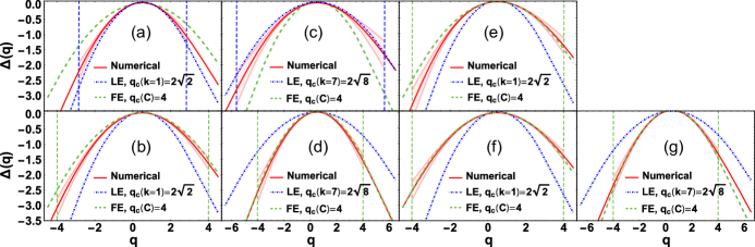
Figure 1: Anomalous part of the multifractal spectrum $\Delta(q)\equiv\tau(q)-2(q-1)$ for low-energy (a,c) and finite-energy (b,d) states, for the TSC surface state model in Eq. (1) with $k=1$ (a,b) and $k=7$ (c,d). The solid red curves obtain from momentum-space exact diagonalization Chou2014 . The blue dot-dashed curve (green dashed curve) is the $k$-dependent (independent) class CI (class C SQH plateau transition) prediction. The solid red curve in each panel is obtained by averaging over states within a narrow energy bin (see text); the shaded red region indicates the standard deviation within the bin. Panel (e) shows the same for low-energy states when time-reversal symmetry is broken explicitly, while spin SU(2) (particle-hole) symmetry is preserved. The disorder strength $\lambda=1.6\pi$ ($16\pi$) for $k=1$ ($7$). Parameters for (e) are specified in Supp . The system is a $(2N+1)\times(2N+1)$ momentum grid; $N=40$ for (a)–(e). Panels (f,g) are the same as (b,d), but for a larger system size ($N=46$).

Numerical Results.—In Fig. 1, we plot the anomalous part of the multifractal spectrum $\Delta(q)\equiv\tau(q)-2(q-1)$ for $k=1$ (a,b) and $k=7$ (c,d). The class CI and class C (percolation) analytical predictions are respectively depicted as blue dot-dashed and green dashed lines. In Figs. 1(a,c), we plot the numerical result for the low-energy states of the spectrum, which show good agreement with the $k$-dependent class CI prediction. Calculations are performed for a typical realization of the random phase disorder, without disorder-averaging, over a square grid of momenta. The solid red line in each panel is obtained by averaging over a narrow energy bin of 36 consecutive low-energy states. For $k=7$ these correspond to the lowest positive energies in the spectrum, while for $k=1$ we neglect states very close to zero energy, keeping those in the energy bin (0.01-0.0141) (see Fig. 2 for the numerical density of states versus energy). The average plus or minus the standard deviation is indicated by the light red shaded region in each panel. We plot the deviation only for $|q|<q_{c}$, where $q_{c}$ is the termination threshold for the low-energy class CI prediction (a,c) or finite-energy SQHE class C prediction (b,d). Since the spectrum becomes linear outside of this range, the error in $\Delta(q)$ also grows linearly for $|q|>q_{c}$, but only the slope discrepancy near $q=\pm q_{c}$ is meaningful.

Figs. 1(b,d) show the results for finite-energy states. For both $k=1$ (b) and $k=7$ (d), the solid red curve in each panel agrees well with the class C prediction (dashed green curve). The finite-energy bin for each $k$ is selected as the one with the highest percentage of states matching the spin quantum Hall prediction, as indicated by a certain fitness criterion described below. Figs. 1(f,g) are the same as Figs. 1(b,d), but for a larger system size.

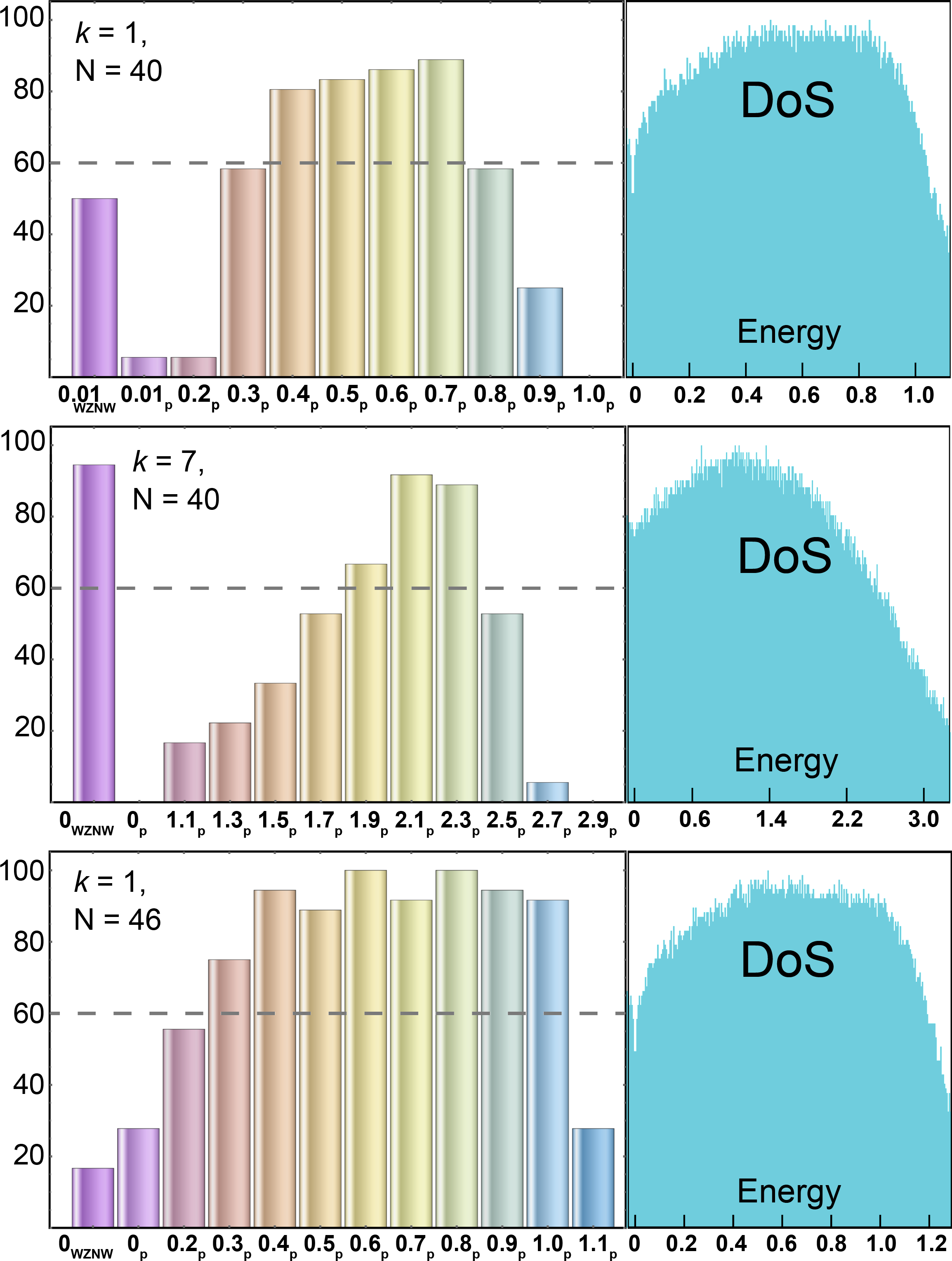
Figure 2: Population statistics for critically delocalized eigenstates. The bars in each graph give the percentage of states with consecutive energy eigenvalues lying within a narrow energy bin that match a certain fitness criterion. The bar labeled “$\mathsf{E}_{\mathsf{WZNW}}$” (“$\mathsf{E}_{\mathsf{P}}$”) denotes the percentage of eigenstates in the bin beginning with energy $\mathsf{E}$ that match the class CI (class C) prediction for the multifractal spectum (see text for details). The bar energy labels should be compared to the corresponding density of states (DoS). The top two plots have $N=40$, while the bottom has $N=46$. In the latter case even the lowest energy bin has more class C than class CI states. The disorder strength $\lambda=1.6\pi$ ($16\pi$) for $k=1$ ($7$).

Fig. 1(e) shows the low-energy spectrum of the $k=1$ model, but now with time-reversal symmetry broken explicitly. This is obtained by turning on random mass and nonabelian potential terms with vanishing average value, but nonzero variance Kagalovsky1999 ; Supp . This preserves spin SU(2) symmetry. A nonzero average mass corresponds to a “spin Hall Chern insulator”; tuning this to zero while retaining a nonzero variance was expected to give the SQHE plateau transition Ryu2009 ; Ryu2012 . Fig. 1(e) matches the states in Figs. 1(b,d,f,g).

In Fig. 2, we compare the computed $\tau(q)$ spectrum for every state in regularly spaced energy bins to the class CI and C predictions, for $k=\{1,7\}$. We introduce a “fitness” criteria, defined as follows. For each eigenstate $\psi(\bm{\mathrm{r}})$, we compute the error between the numerical spectrum [$\equiv\tau_{N}(q)$] and the appropriate analytical prediction [$\equiv\tau_{A}(q)$], error$(q)\equiv|\tau_{N}(q)-\tau_{A}(q)|/\tau_{A}(q)$. If the error is less than or equal to 6% for 75% of the evaluated $q$-points in the interval $0\leq q\leq q_{c}$, we keep the state. We consider bins of 36 states each; the states within each bin have consecutive eigenenergies. The height of each bar marked “$\mathsf{E}_{\mathsf{WZNW}}$” (“$\mathsf{E}_{\mathsf{P}}$”) denotes the percentage of eigenstates in the bin starting with energy $\mathsf{E}$ that match the class CI (class C) prediction. The energies in each left panel of Fig. 2 should be compared to the numerical density of states shown in the corresponding right panel.

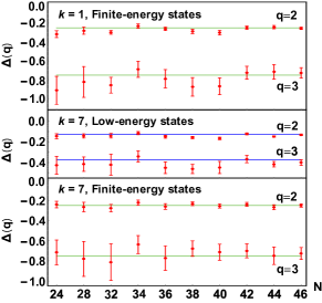
Figure 3: Finite-energy and low-energy $\Delta(q)$ as in Fig. 1, but for fixed $q=2,3$ and for varying system sizes $N$. The intrinsic disorder correlation length and strength are kept fixed Supp . The blue and green lines are the exact analytical predictions for $\Delta(2,3)$ Foster2012 ; Mirlin2003 . The solid points show the average, while error bars indicate the standard deviation within the energy bin. The main effect of increasing $N$ is to reduce the fluctuations, although the reduction is slower for $q$ closer to $q_{c}$ ($=4$ for class C). See Supp for full $\Delta(q)$ and population statistics.

Fig. 2 indicates that for $k=1$ the finite energy states match well the class C SQH prediction (bins $\mathsf{E}_{\mathsf{P}}$ with $\mathsf{E}\in\{0.4,\ldots,0.7\}$ for $N=40$). The plot for $k=7$ shows a narrower band of finite energy states that match class C for the chosen disorder strength; results for $k=8$ are similar Supp . Results for a larger $k=1$ system ($N=46$) appear at the bottom of Fig. 2, showing that the statistics at finite energy improve with increasing system size.

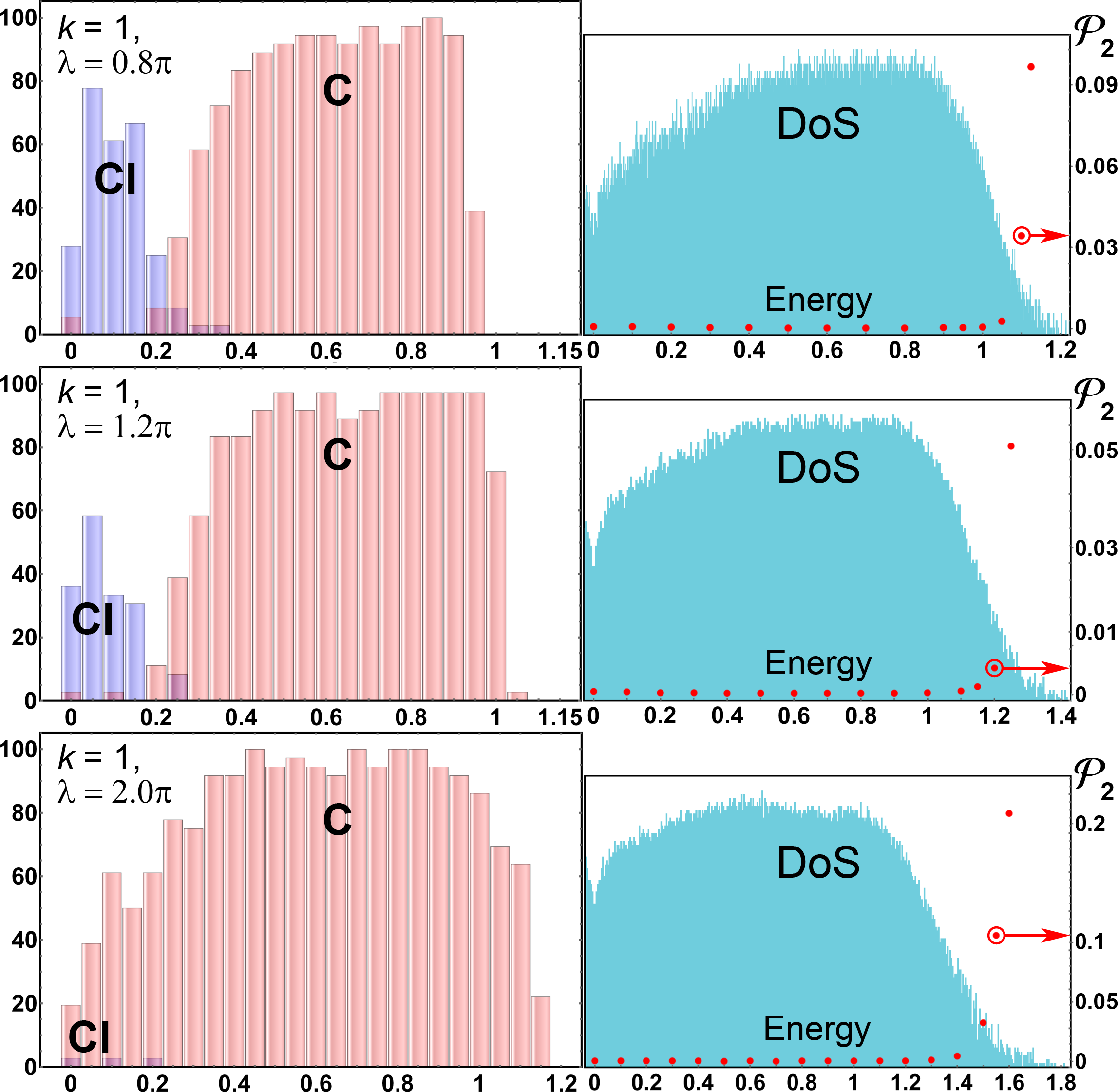
Figure 4: Disorder strength ($\lambda$)-dependence of the population statistics for $k=1$. Blue (red) bars marked CI (C) describe the percentage of states that match the class CI (C) multifractal spectrum; results are shown for $\lambda\in\{0.8,1.2,2.0\}\pi$ and $N=46$. $\lambda=2\pi$ corresponds to strong disorder (the freezing transition for the abelian AIII model Ludwig1994 ; Chou2014 ; Chamon1996 ). The main effect of increasing $\lambda$ is to decrease the percentage of CI-like states. The second IPR $\mathcal{P}_{2}$ (red dots) is superimposed over the associated DoS in the right-hand plots. Even for strong disorder, this becomes appreciable only in the high-energy “Lifshitz tail,” possibly signaling localization there LocNote .

The finite-energy results for $\tau(q)$ shown in Figs. 1(b,d,f,g) were obtained from the bin with the highest percentage of states matching the class C SQH prediction for each value of $k$. I.e., for $k=7$, the red solid curve in Fig. 1(d) was obtained by averaging over states in the bin starting with energy $\mathsf{E}=2.1$ (Fig. 2). We emphasize that while the fitness criterion introduced above is arbitrary, the trends are not Supp .

We show finite-size trends in Fig. 3. Here we plot $\Delta(q)$ for $q=2,3$, which are well-distinguished for the class CI (low-energy) and class C (finite-energy) analytical predictions Foster2012 ; Mirlin2003 . The trends for increasing $N$ suggest convergence towards the analytical results.

Population statistics (computed as in Fig. 2) for variable disorder are shown in Fig. 4. Stronger disorder converts more of the low-energy spectrum from class CI to class C in a fixed system size. We also plot the second inverse participation ratio $\mathcal{P}_{2}$, which becomes appreciable only in the high-energy tail. Since $\mathcal{P}_{2}\sim\zeta^{-2}$ for a state with localization length $\zeta$ Huckestein1995 ; Evers2008 , localization (if it occurs LocNote ) is restricted to high energies, and does not encroach upon the wide “multifractal spin metal” class C region.

Conclusion.—Our results are completely different from a 2D system with delocalization at only one energy, as in the quantum Hall plateau transition Huckestein1995 . Although localized states arbitrarily close to that transition appear critical on large scales, the criticality reflects the transition itself. By contrast, here we find (1) the expected class CI criticality near zero energy, and (2) a robust, completely different, non-standard class C criticality over a wide swath of finite energy states. This swath does not shrink as the disorder strength or system size is increased.

Although we observe “localization” LocNote in the high-energy tail (Fig. 4), we believe that this is an artifact of the unphysical UV truncation of the TSC surface Hamiltonian. A real 3D TSC would hybridize 2D surface states with the bulk when the surface energy crosses the bulk gap. We expect that all states in this case are delocalized, and that all of the 2D surface states below the gap show class C criticality (except the one at zero energy).

The class CI zero energy state is described by a Wess-Zumino-Novikov-Witten (WZNW) nonlinear sigma model Foster2012 ; Foster2014 . The energy perturbation breaks the symmetry from $G\times G$ down to $G$, where $G=\text{Sp}(4n)$ (using replicas, with $n\rightarrow 0$). This relevant perturbation presumably induces a renormalization group (RG) flow to another sigma model with lower symmetry. This argument is insufficient to choose between the orthogonal metal class AI [manifold $\text{Sp}(4n)/\text{Sp}(2n)\times\text{Sp}(2n)$] and class C [manifold $\text{Sp}(4n)/\text{U}(2n)$] Evers2008 . If the class CI model is deformed to class C “by hand,” the WZNW term becomes a theta term (with theta proportional to $k$) Supp .

We thank Ilya Gruzberg, Victor Gurarie, Lucas Wagner, Robert Konik, Alexei Tsvelik, Antonello Scardicchio, Vadim Oganesyan, and Sarang Gopalakrishnan for useful discussions. This research was supported by the Welch Foundation grants No. E-1146 (S.A.A.G.) and No. C-1809 (Y.L. and M.S.F.), as well as NSF CAREER Grant No. DMR-1552327 (Y.L. and M.S.F.), and by the Texas center for the superconductivity (S.A.A.G.). M.S.F. thanks the Aspen Center for Physics, which is supported by the NSF Grant No. PHY-1066293, for its hospitality while part of this work was performed.

Critical Percolation Without Fine Tuning on the Surface of a Topological Superconductor
SUPPLEMENTAL MATERIAL

I I. Particle-hole symmetry for odd and even $k$

The Hamiltonian $\hat{h}$ can be succinctly encoded by introducing an additional species of Pauli matrices $\hat{\sigma}^{1,2,3}$ as a basis for the decomposition in Eq. (1). Then

$$\hat{h}=\frac{1}{2}\left[\hat{\sigma}^{+}\left(-i\partial\right)^{k}+\hat{\sigma}^{-}\left(-i\bar{\partial}\right)^{k}\right]+\hat{\bm{\sigma}}\cdot\bm{\mathrm{A}}^{a}(\bm{\mathrm{r}})\,\hat{\tau}^{a}+\hat{\bm{\sigma}}\cdot\bm{\mathrm{A}}^{0}(\bm{\mathrm{r}}),$$ (S1)

where $\hat{\sigma}^{\pm}\equiv\hat{\sigma}^{1}\pm i\hat{\sigma}^{2}$ and $\hat{\bm{\sigma}}\cdot\bm{\mathrm{A}}=\hat{\sigma}^{1}A_{x}+\hat{\sigma}^{2}A_{y}$. Physical time-reversal invariance is encoded in the chiral condition S–SRFL2008 ; S–Foster2012 ; S–Foster2014

$$-\hat{M}_{\mathsf{S}}\,\hat{h}\,\hat{M}_{\mathsf{S}}=\hat{h},\qquad\hat{M}_{\mathsf{S}}=\hat{\sigma}^{3}.$$ (S2)

For class CI, particle-hole symmetry $P$ must involve an antisymmetric matrix $\hat{M}_{\mathsf{P}}=-\hat{M}_{\mathsf{P}}^{\mathsf{T}}$ (“$P^{2}=-1$”) S–SRFL2008 . The particle-hole condition is

$$-\hat{M}_{\mathsf{P}}\,\hat{h}^{\mathsf{T}}\,\hat{M}_{\mathsf{P}}=\hat{h},$$ (S3)

where $\mathsf{T}$ denotes the transpose operation and it is understood that derivative operators are odd under transposition: $(\partial_{x,y})^{\mathsf{T}}=-\partial_{x,y}$.

For $k\in\{1,3,5,\ldots\}$ (odd), we take S–Foster2012 ; S–Foster2014

$$\hat{M}_{\mathsf{P}}^{{\scriptscriptstyle{(\mathsf{{odd}})}}}=\hat{\sigma}^{1}\hat{\tau}^{2}.$$ (S4)

Eq. (S1) is invariant under Eq. (S3) with this choice provided we set the abelian vector potential equal to zero, $\bm{\mathrm{A}}^{0}=0$. For $k\in\{2,4,6,\ldots\}$ (even), we take

$$\hat{M}_{\mathsf{P}}^{{\scriptscriptstyle{(\mathsf{{even}})}}}=\hat{\sigma}^{2}\hat{\tau}^{1}.$$ (S5)

Eq. (S1) is invariant under Eq. (S3) with this choice provided we set the third component of the SU(2) vector potential equal to zero, $\bm{\mathrm{A}}^{3}=0$.

II II. Class C model with broken TRI

In Fig. 1(e), we exhibit the low-energy anomalous multifractal spectrum $\Delta(q)=\tau(q)-2(q-1)$ for the $k=1$ class CI model in Eq. (S1), except that we have now explicitly broken time-reversal symmetry (in every fixed realization of disorder, but not on average). The Hamiltonian in this case resides in class C S–Kagalovsky1999 ,

$$\hat{h}_{\scriptscriptstyle{\mathrm{C}}}\equiv\hat{h}+m(\bm{\mathrm{r}})\,\hat{\sigma}^{3}+v^{a}(\bm{\mathrm{r}})\,\hat{\tau}^{a},$$ (S6)

where $a\in\{1,2,3\}$. The mass $m(\bm{\mathrm{r}})$ and nonabelian valley potentials $v^{1,2,3}(\bm{\mathrm{r}})$ break physical time-reversal symmetry [Eq. (S2)], but preserve $P^{2}=-1$ particle-hole [Eqs. (S3) and (S4) for $k=1$]. The latter is tantamount to spin SU(2) invariance.

III III. Parameter specification for the numerics

The numerical results presented in Figs. 1–4 were obtained via the exact diagonalization of $\hat{h}$ in Eq. (1). Calculations are performed in momentum space. All disorder potentials are parameterized as described in the text, i.e.

$$A_{i}^{\mu}(\bm{\mathrm{q}})=\frac{\sqrt{\lambda}}{L}\exp\left[i\,\theta_{i}^{\mu}(\bm{\mathrm{q}})-\frac{q^{2}\xi^{2}}{4}\right],$$ (S7)

where $i\in\{x,y\}$ and $\mu\in\{0,1,2,3\}$. The phases $\theta_{i}^{\mu}(\bm{\mathrm{q}})=-\theta_{i}^{\mu}(-\bm{\mathrm{q}})$, but are otherwise identical, independent random variables uniformly distributed over $[0,2\pi)$. This approach is equivalent to disorder-averaging, up to finite-size corrections S–Chou2014 . We assign the same disorder strength $\lambda$ to all nonzero components of the abelian $\mathsf{A}^{0}$ and nonabelian $\mathsf{A}^{1,2,3}$ vector potentials. We choose $\lambda=1.6\pi$ ($16\pi$) for the $k=1$ ($k=7$) calculations with $N=40$ [except Fig. 1(e), described below]. Different disorder strengths are studied in Fig. 4 (with $N=46$), as described in the caption to that figure.

The arbitrary dimensionful system length $L$ determines the ultraviolet cutoff $\Lambda=2\pi N/L$. The correlation length of the impurity potentials is chosen to be $\xi=0.25(L/N)$ S–Chou2014 . For $N\neq 40\equiv N_{0}$ in Figs. 1–3, we rescale the disorder parameter $\lambda\rightarrow(N/N_{0})^{2(k-1)}\lambda$, which corresponds to fixing the intrinsic disorder strength relative to the appropriate power of the momentum cutoff. There is no rescaling in the $k=1$ (Dirac dispersion) case, where $\lambda$ is dimensionless.

The multifractal spectra exhibited in Figs. 1(a,b,e) and (c,d) are extracted using box sizes $b=2$ and $b=8$ ($k=1$) and $b=3$ and $b=10$ ($k=7$), respectively. Box sizes for Figs. 1(f,g) are $b=2$ and $b=13$ ($k=1$) and $b=2$ and $b=31$ ($k=7$).

For the low-energy states in class C with $k=1$ [Fig. 1(e)], in addition to the nonabelian vector potentials $A_{x,y}^{1,2,3}$, we include random mass $m(\bm{\mathrm{r}})$ and (valley-graded) scalar potential $v^{3}(\bm{\mathrm{r}})$ disorders, see Eq. (S6). The disorder strengths are $\lambda_{A}=\lambda_{v^{3}}=0.8\pi$, while the mass variance is $\lambda_{m}=16\pi$. We neglect the off-diagonal potentials $v^{1,2}(\bm{\mathrm{r}})=0$ [Eq. (S6)].

IV IV. Sigma models for class CI TSC surface states and the class C SQHE

The nonlinear sigma model representations for (a) the class CI conformal field theory describing zero-energy TSC surface state wave functions and (b) the class C spin quantum Hall effect are captured by the following actions S–Senthil1998 ; S–Foster2014 ; S–Liao2017 ,

$$S_{\scriptscriptstyle{\mathrm{CI}}}= \,\frac{k}{8\pi}\int d^{2}\bm{\mathrm{r}}\operatorname{Tr}\left[\bm{\nabla}\hat{q}^{\dagger}\cdot\bm{\nabla}\hat{q}\right]+i\,\frac{\omega}{2}\int d^{2}\bm{\mathrm{r}}\operatorname{Tr}\left[\hat{\Lambda}\left(\hat{q}+\hat{q}^{\dagger}\right)\right]-i\frac{k}{12\pi}\int d^{2}\bm{\mathrm{r}}\,dR\,\epsilon^{abc}\operatorname{Tr}\left[\left(\hat{q}^{\dagger}\partial_{a}\hat{q}\right)\left(\hat{q}^{\dagger}\partial_{b}\hat{q}\right)\left(\hat{q}^{\dagger}\partial_{c}\hat{q}\right)\right],$$ (S8a)

$$S_{\scriptscriptstyle{\mathrm{C}}}= \,\frac{\sigma_{11}}{8}\int d^{2}\bm{\mathrm{r}}\operatorname{Tr}\left[\bm{\nabla}\hat{q}\cdot\bm{\nabla}\hat{q}\right]+i\,\omega\int d^{2}\bm{\mathrm{r}}\operatorname{Tr}\left[\hat{\Lambda}\,\hat{q}\right]-\frac{\sigma_{12}}{8}\int d^{2}\bm{\mathrm{r}}\,\epsilon^{ij}\operatorname{Tr}\left[\hat{q}\,\partial_{i}\,\hat{q}\,\partial_{j}\,\hat{q}\right].$$ (S8b)

In Eq. (S8a), $\hat{q}(\bm{\mathrm{r}})$ is a $4n\times 4n$ unitary matrix field that is also a $\text{Sp}(4n)$ group element; $\bm{\mathrm{r}}=\{x,y\}$ is the position vector that spans over the 2D TSC surface. We assume that disorder-averaging has been accomplished with the replica trick; $n\rightarrow 0$ counts the number of replicas S–Altland . Here and in Eq. (S8b), $\omega$ is a real parameter that denotes the ac frequency of the spin conductivity that the sigma model is designed to compute S–Liao2017 ; S–Altland . The matrix $\hat{\Lambda}$ is diagonal and equal to $\hat{\Lambda}=\mathrm{diag}(1,1,\ldots,1,-1,-1,\ldots,-1)$ [$2n$ (+1)s and $2n$ (-1)s]. The last term in Eq. (S8a) is the Wess-Zumino-Novikov-Witten (WZNW) term. This term is defined over a three-dimensional ball (coordinates $\{\bm{\mathrm{r}},R\}$, $0\leq R\leq 1$), such that $\hat{q}(\bm{\mathrm{r}},R=1)=\hat{q}(\bm{\mathrm{r}})$ is the field on the 2D surface, while $\hat{q}(\bm{\mathrm{r}},R)$ for $R<1$ is a smooth deformation of this into the ball interior. The WZNW term ensures that the action in Eq. (S8a) is conformally invariant for $\omega=0$ S–Foster2014 ; S–BYB . In the context of a 3D topological superconductor, the ball can be identified with the bulk if the surface has genus zero S–Konig2012 .

The structure of the first two terms of the class C sigma model can be obtained from the corresponding ones in class CI by imposing the additional constraint on $\hat{q}(\bm{\mathrm{r}})$ by hand,

$$\hat{q}^{\dagger}(\bm{\mathrm{r}})=\hat{q}(\bm{\mathrm{r}}).$$ (S9)

The matrix $\hat{q}(\bm{\mathrm{r}})$ now belongs to the space $\text{Sp}(4n)/\text{U}(2n)$ S–Senthil1998 ; S–Evers2008 . The last term in Eq. (S8b) is the Pruisken or theta term, which assigns winding numbers to different topological sectors of the $\hat{q}$-field and evaluates to a pure imaginary phase S–Altland . The coefficients of the first and third terms in Eq. (S8b) are respectively proportional to the longitudinal conductivity $\sigma_{11}$ and Hall conductivity $\sigma_{12}$; the class CI WZNW model has $\sigma_{11}=k/\pi$ and $\sigma_{12}=0$ (in units of the spin conductance quantum) S–SRFL2008 ; S–Foster2014 .

When the constraint in Eq. (S9) is imposed on $\hat{q}(\bm{\mathrm{r}})$ in Eq. (S8a), we can show that the WZNW term in the latter becomes the theta term in Eq. (S8b), with

$$\sigma_{12}=k/2.$$ (S10)

However, we stress that in the context of the finite-energy TSC surface states discussed in this Letter, there is no reason to trust this assignment of $\sigma_{12}$, because it does not follow from a physical RG flow. As emphasized at the end of the main text, the only statement we can make is that the energy perturbation (the operator coupling to $\omega\neq 0$) is relevant, and breaks the symmetry of the class CI model from $G\times G$ down to $G$, where $G=\text{Sp}(4n)$ S–Footnote .

If $\omega\neq 0$ induces a flow to the class C SQHE plateau transition, it is must be due to the effect of the WZNW term on the RG. Without the WZNW term, the class CI model describes (gapless) quasiparticles in an ordinary (non-topological) spin-singlet superconductor, and the single-particle wave functions must become those of the orthogonal metal class AI at large energies. Moreover, in this case all states (at zero and finite energy) are localized in 2D for arbitrarily weak disorder S–Senthil1998 ; S–Evers2008 .

IV.1 A. From WZNW to theta

The derivation of Eq. (S10) requires a little care, since the restriction in Eq. (S9) induces topologically distinct sectors of the $\hat{q}$-matrix; this is why the theta term in Eq. (S8b) can produce an effect. It means that the field $\hat{q}(\bm{\mathrm{r}},R)$ appearing in the WZNW term of Eq. (S8a) cannot be strictly restricted in this way, because otherwise it is not possible to deform generic $\hat{q}(\bm{\mathrm{r}},R<1)$ in the interior to some particular $\hat{q}(\bm{\mathrm{r}},R=1)$ at the surface. Here we show how the WZNW term in Eq. (S8a) becomes the theta term in Eq. (S8b), employing the method used in Ref. S–Bocquet2000 .

We extend $\hat{q}(\bm{\mathrm{r}})$ on the 2D surface to $\hat{q}(\bm{\mathrm{r}},R)$ on the three-dimensional ball through the following equation:

$$\begin{aligned} \hat{q}(\bm{\mathrm{r}},R)=\,&-i\cos\left(\frac{\pi R}{2}\right)\hat{1}+\sin\left(\frac{\pi R}{2}\right)\hat{q}(\bm{\mathrm{r}}),\qquad 0\leq R\leq 1.\end{aligned}$$ (S11)

In this extension scheme, we have $\hat{q}(\bm{\mathrm{r}},R=0)=-i\hat{1}$ (where $\hat{1}$ is the identity) and $\hat{q}(\bm{\mathrm{r}},R=1)=\hat{q}(\bm{\mathrm{r}})$. Note that, unlike $\hat{q}(\bm{\mathrm{r}})$ on the surface, $\hat{q}(\bm{\mathrm{r}},R)$ does not obey the restriction in Eq. (S9).

Inserting Eq. (S11) into the WZNW term of Eq. (S8a), the latter reduces to

$$\begin{aligned} &-\frac{k}{8}\int d^{2}\bm{\mathrm{r}}\,dR\,\epsilon^{abc}\operatorname{Tr}\left[\hat{q}(\bm{\mathrm{r}})\partial_{b}\hat{q}(\bm{\mathrm{r}})\partial_{c}\hat{q}(\bm{\mathrm{r}})\right]\sin^{2}\left(\frac{\pi R}{2}\right)\partial_{a}R\\ =\,&-\frac{k}{8}\int d^{2}\bm{\mathrm{r}}\,dR\,\epsilon^{abc}\operatorname{Tr}\left\{\partial_{a}\left[\hat{q}(\bm{\mathrm{r}})\partial_{b}\hat{q}(\bm{\mathrm{r}})\partial_{c}\hat{q}(\bm{\mathrm{r}})\left(\frac{R}{2}-\frac{1}{2\pi}\sin(\pi R)\right)\right]\right\}\\ =\,&-\frac{k}{16}\int d^{2}\bm{\mathrm{r}}\,\epsilon^{ij}\operatorname{Tr}\left[\hat{q}(\bm{\mathrm{r}})\partial_{i}\hat{q}(\bm{\mathrm{r}})\partial_{j}\hat{q}(\bm{\mathrm{r}})\right],\end{aligned}$$ (S12)

where in the second equality we have used the divergence theorem and the fact that $R=1$ on the 2D surface. Comparing this expression with the theta term in Eq. (S8b), one obtains Eq. (S10).

V V. Additional numerical results

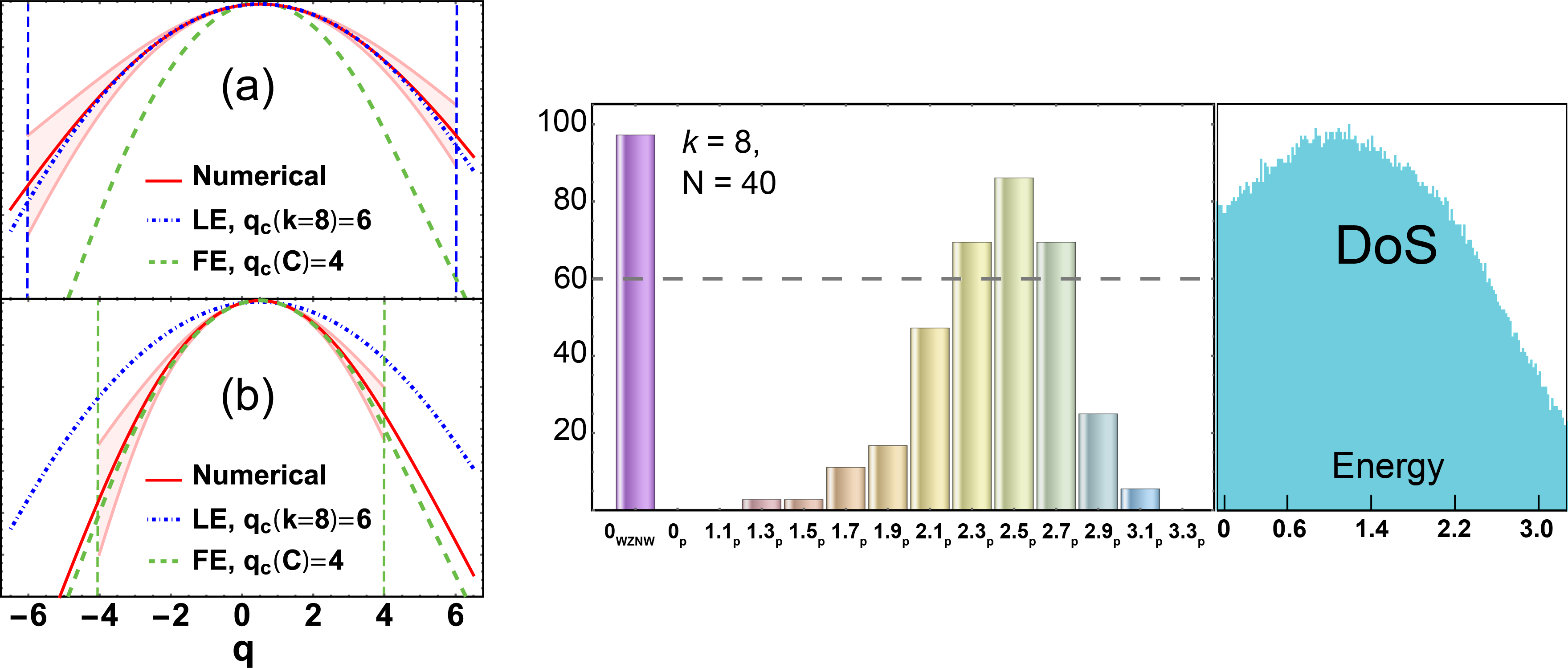
Figure S1: Results for $k=8$ and $N=40$. Left: anomalous part of the multifractal spectrum $\Delta(q)\equiv\tau(q)-2(q-1)$ as in Fig. 1 of the main text. The top panel (a) [bottom panel (b)] shows the low-energy (finite-energy) states, compared to the analytical predictions for class CI (blue dot-dashed curve) and class C (green dashed curve). The right panel shows the population statistics for critically delocalized eigenstates as in Fig. 2 of the main text.

V.1 A. $k=8$ results

Our results in this Letter generalize a previous observation for a simpler model in class AIII. This model consists of a single 2D Dirac fermion coupled to abelian vector potential disorder; it is critically delocalized and exactly solvable at zero energy S–Ludwig1994 . It can also be interpreted as the surface state of TSC with winding number $\nu=1$ S–SRFL2008 ; S–Foster2014 . It was claimed S–Ostrovsky2007 that all finite-energy states of this model should reside at the plateau transition of the (class A) integer quantum Hall effect, and this was verified numerically S–Chou2014 . The same logic employed by Haldane S–Haldane-EO and Pruisken S–Pruisken-EO implies that there should be an “even-odd” effect whereby AIII surface states for a TSC with even winding number are localized at finite energy, while those with odd form stacks of critical plateau-transition states S–Ostrovsky2007 . Here we find critical delocalization for all class CI winding numbers, with no “even-odd” effect.

Results for $k=8$ and $N=40$ are shown in Fig. S1. The box sizes chosen to obtain the multifractal spectrum are $b=5$ and $b=10$.

V.2 B. Density of states

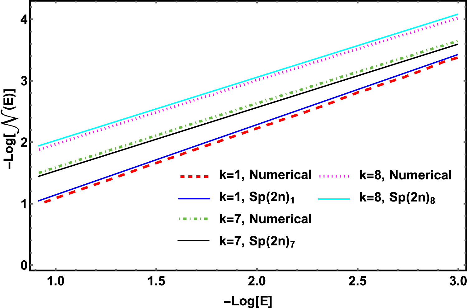
Figure S2: Log-log plot of the integrated density of states $\mathcal{N}(\mathsf{E})$ obtained via exact diagonalization of $\hat{h}$ in Eq. (1), versus the exact analytical prediction of the class CI conformal field theory S–LeClair2008 ; S–Foster2012 . Results are shown for $k=\{1,7,8\}$, with parameters chosen the same as in Figs. 1, 2, and S1 ($N=40$).

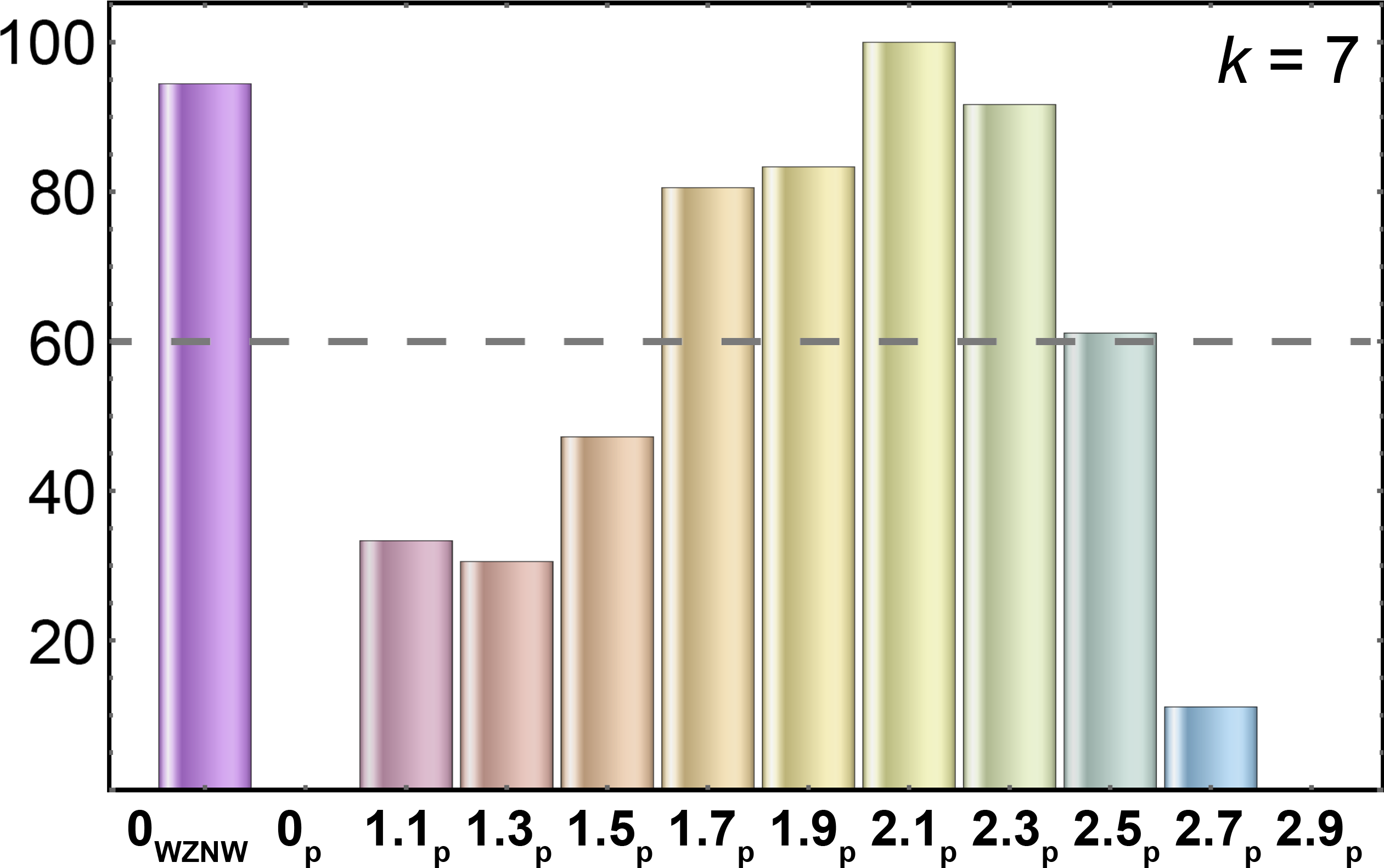
Figure S3: The same as the second left-hand panel of Fig. 2 ($k=7$), but with a 7% error threshold for states matching the class CI (“WZNW”) or C (“P”) prediction for the multifractal spectrum $\tau(q)$, over the range $0\leq q\leq q_{c}$.

The numerical density of states (DoS) is depicted via the histograms in the right panels of Fig. 2 for $k\in\{1,7\}$ and in Fig. S1 for $k=8$. The DoS shows a “dip” upon approaching zero energy $\mathsf{E}=0$. This is expected for the critically delocalized class CI surface states, where the $\text{Sp}(2n)_{k}$ conformal field theory predicts universal scaling for the DoS $\nu(\mathsf{E})$ S–LeClair2008 ; S–Foster2012

$$\nu(\mathsf{E})\sim|\mathsf{E}|^{1/(4k+3)},$$ (S13)

a result that is independent of the multifractal spectrum S–Foster2012 ; S–Foster2014 . In Fig. S2, we compare the numerical integrated density of states $\mathcal{N}(\mathsf{E})\equiv\int^{\mathsf{E}}\nu(\mathsf{E}^{\prime})\,d\mathsf{E}^{\prime}$ to the class CI prediction, and observe good agreement for $k=\{1,7,8\}$ ($N=40$).

V.3 C. Alternative fitness threshold

To obtain the population statistics exhibited in Fig. 2, we employ an arbitrary “fitness” criteria, described in the main text. While the exact percentages of states above the fitness threshold (encoded in the bar heights in Fig. 2) depend somewhat sensitively on these criteria, the overall trends as a function of energy $\mathsf{E}$ do not. In Fig. S3, we replot the same data as in $k=7$ panel of Fig. 2, but for the criterion that a state is kept if it matches the appropriate analytical prediction for $\tau(q)$ with no more than 7% error, over 75% or more of the $q$-values in the range $0\leq q\leq q_{c}$.

V.4 D. Representative class C and high-energy tail-state wave functions for $k=1$, $N=46$

Here we plot representative wave function probability profiles for $k=1$ and $N=46$, for two different disorder strengths $\lambda=\{1.2,2.0\}\pi$. The corresponding population statistics, density of states, and second inverse participation ratio $\mathcal{P}_{2}$ are shown in Fig. 4 of the main text. The latter figure demonstrates that only states deep in the high-energy “tail” exhibit appreciable $\mathcal{P}_{2}$. We therefore expect that these states could exhibit Anderson localization.

Fig. S4 shows that while representative states in the class C “bulk” are clearly critically delocalized, the behavior of the tail states is less clear. In fact, it is possible that the tail states are becoming frozen instead of localized. A single frozen state is “quasilocalized,” and consists of a few peaks that are separated by arbitrarily large distances S–Chamon1996 ; S–Foster2009 . These states are known to arise for class AIII surface states with winding number $\nu=1$ and strong disorder ($\lambda\geq 2\pi$) S–Chamon1996 ; S–Chou2014 .

We do not pursue the nature of the tail states further in this work, since we believe that these are an artifact of the UV cutoff. For 2D surface states attached to a 3D topological superconducting bulk, surface states with energies approaching the gap would bleed into the bulk, ultimately hybridizing with bulk quasiparticles states.

(a) $\lambda=1.2\pi$, Energy $0.75$

(b) $\lambda=1.2\pi$, Energy $1.15$

(c) $\lambda=1.2\pi$, Energy $1.2$

(d) $\lambda=1.2\pi$, Energy $1.25$

(e) $\lambda=2.0\pi$, Energy $0.7$

(f) $\lambda=2.0\pi$, Energy $1.4$

(g) $\lambda=2.0\pi$, Energy $1.5$

(h) $\lambda=2.0\pi$, Energy $1.6$

Figure S4: Representative wave function position space probability profiles $|\psi(\bm{\mathrm{r}})|^{2}$ for $k=1$, $N=46$, and disorder strengths $\lambda=1.2\pi$ and $2.0\pi$ (see Fig. 4 in the main text). The wave functions (a) and (e) are representative of class C multifractal states. The other states reside in the high-energy tail of the DoS (see Fig. 4), which we have argued arises from the unphysical truncation of the surface state spectrum. While the states (d) and (h) appear localized, the intermediate states suggest that the tail states might instead exhibit multifractal freezing S–Chamon1996 ; S–Foster2009 .

V.5 E. Finite-size trends for $k=1$ and $k=7$

Here we plot the anomalous spectrum $\Delta(q)=\tau(q)-2(q-1)$ for low- and finite-energy states as in Fig. 1, as well as the population statistics and numerical density of states as in Fig. 2, for the full range of $N$ used to obtain the results shown in Fig. 3. Box sizes for multifractal analysis are chosen to be almost commensurate with the linear system size $2N+1$.

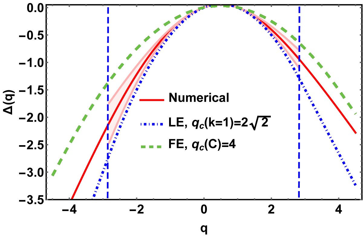
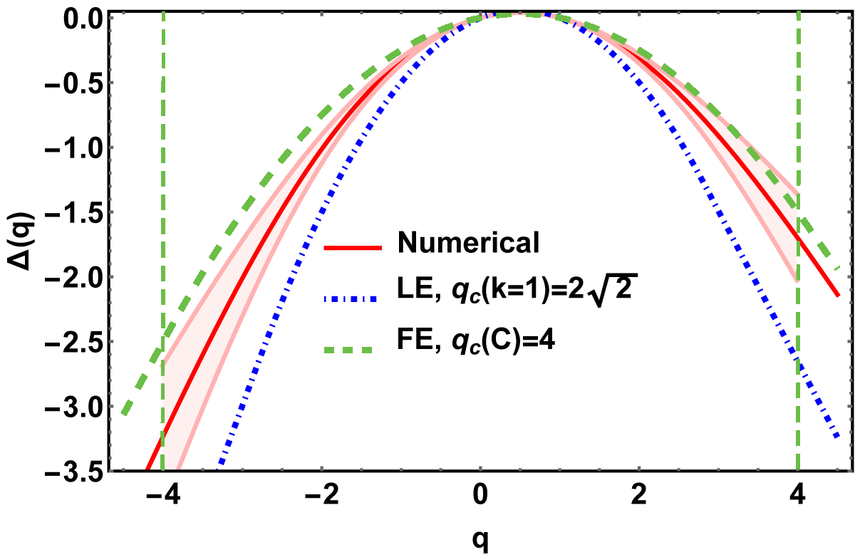
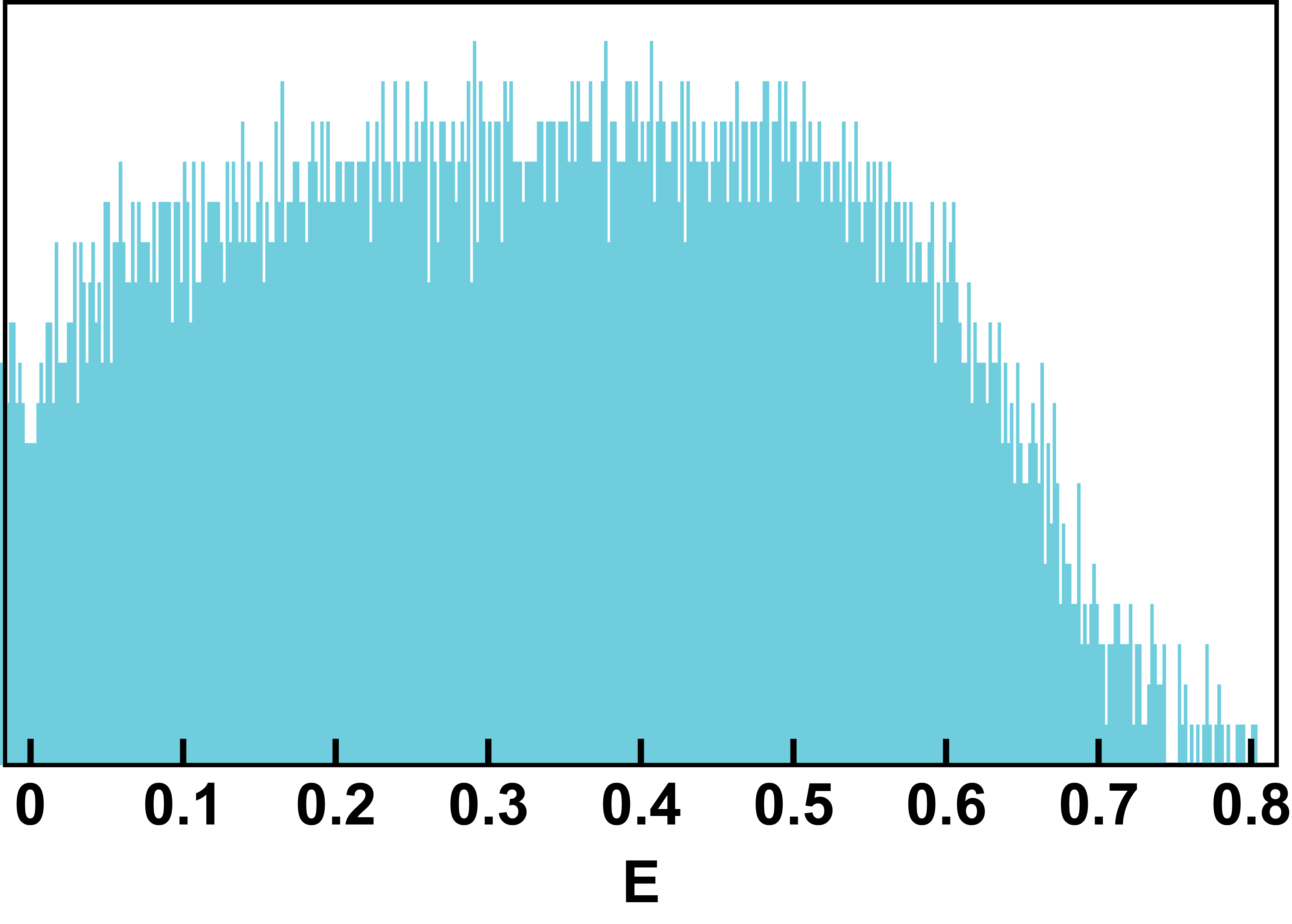
Figure S5: $k=1$, $N=24$. Box sizes $b=2,6$.

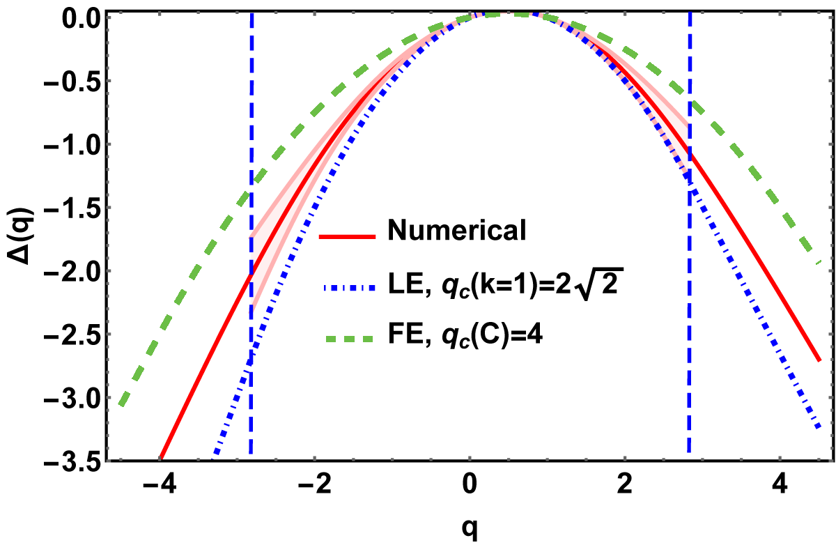
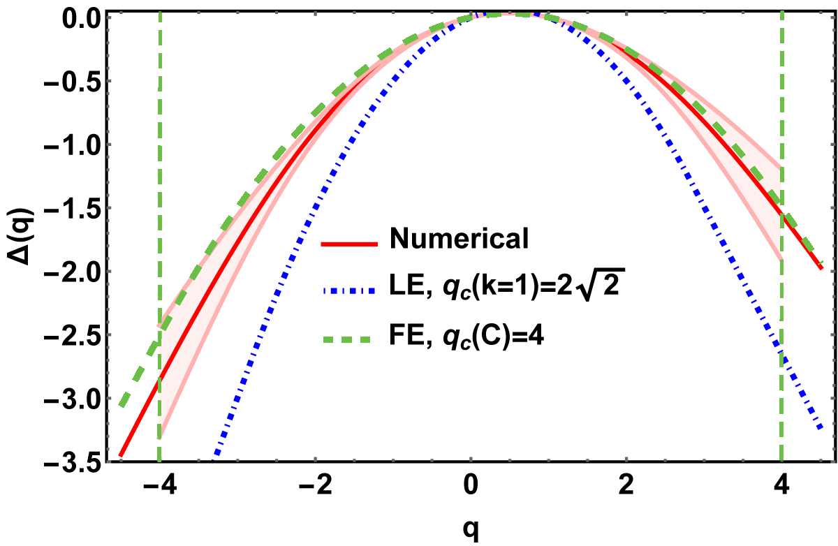
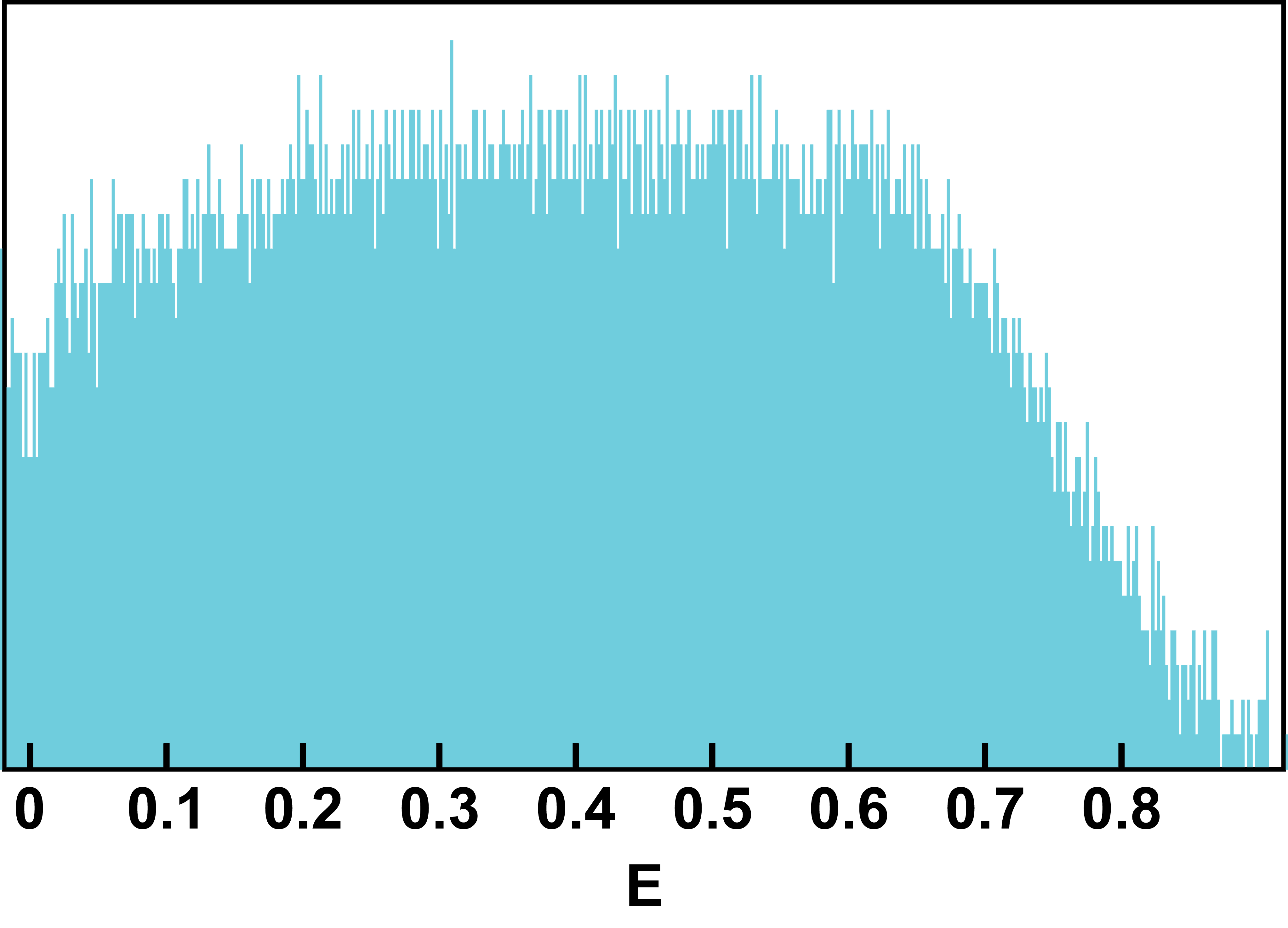
Figure S6: $k=1$, $N=28$. Box sizes $b=2,8$.

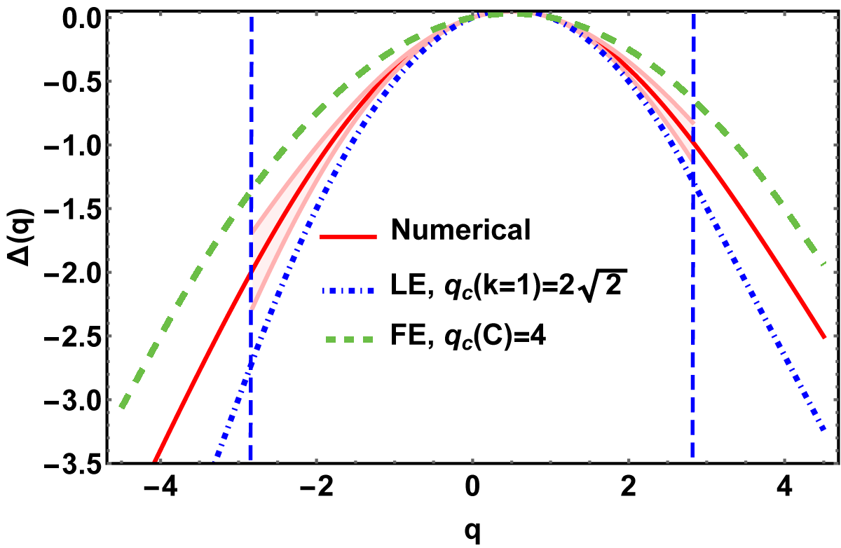
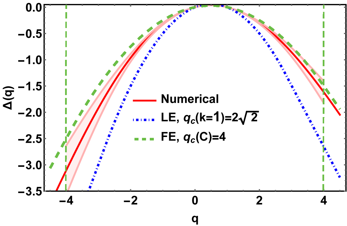
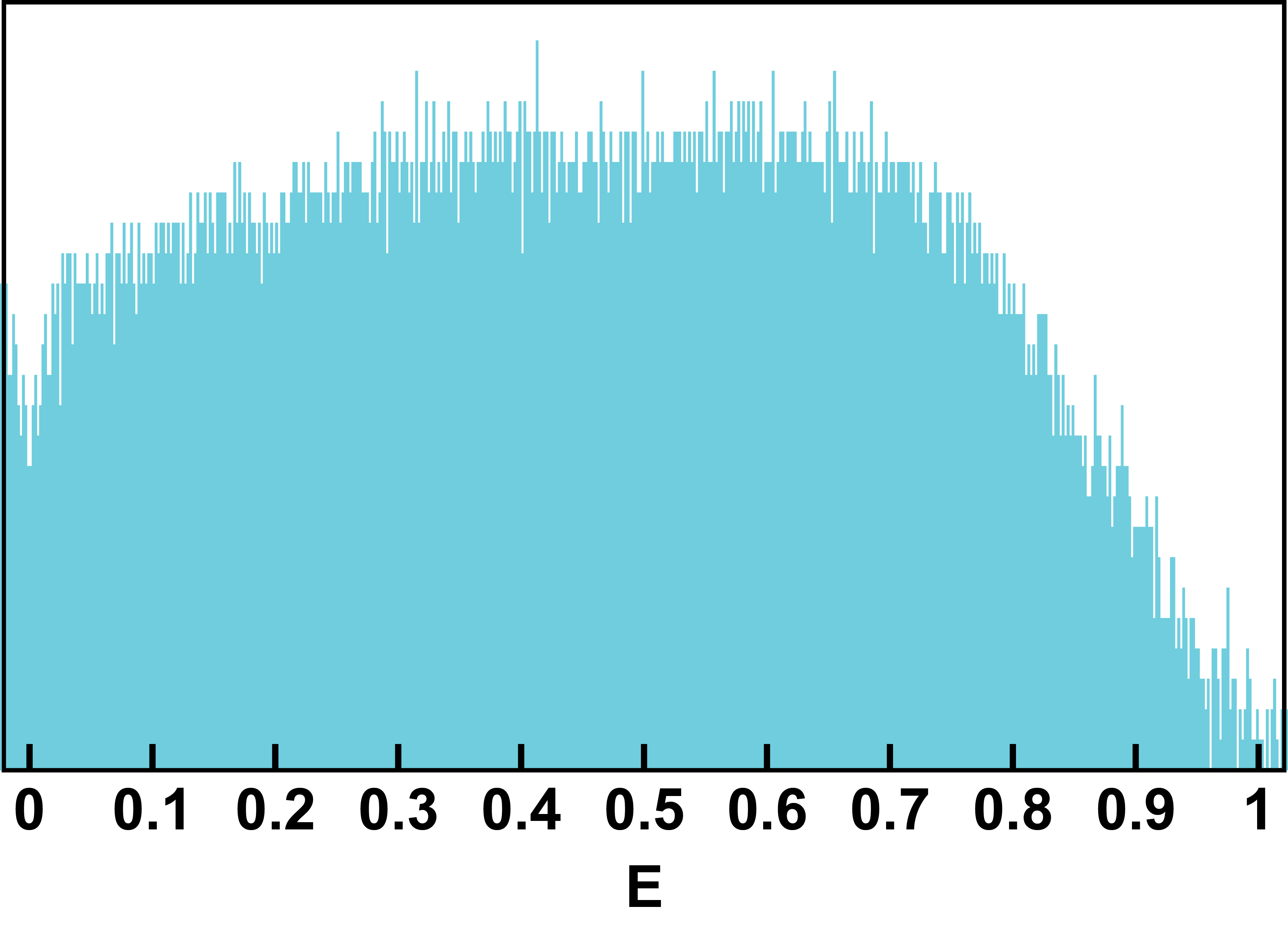
Figure S7: $k=1$, $N=32$. Box sizes $b=2,8$.

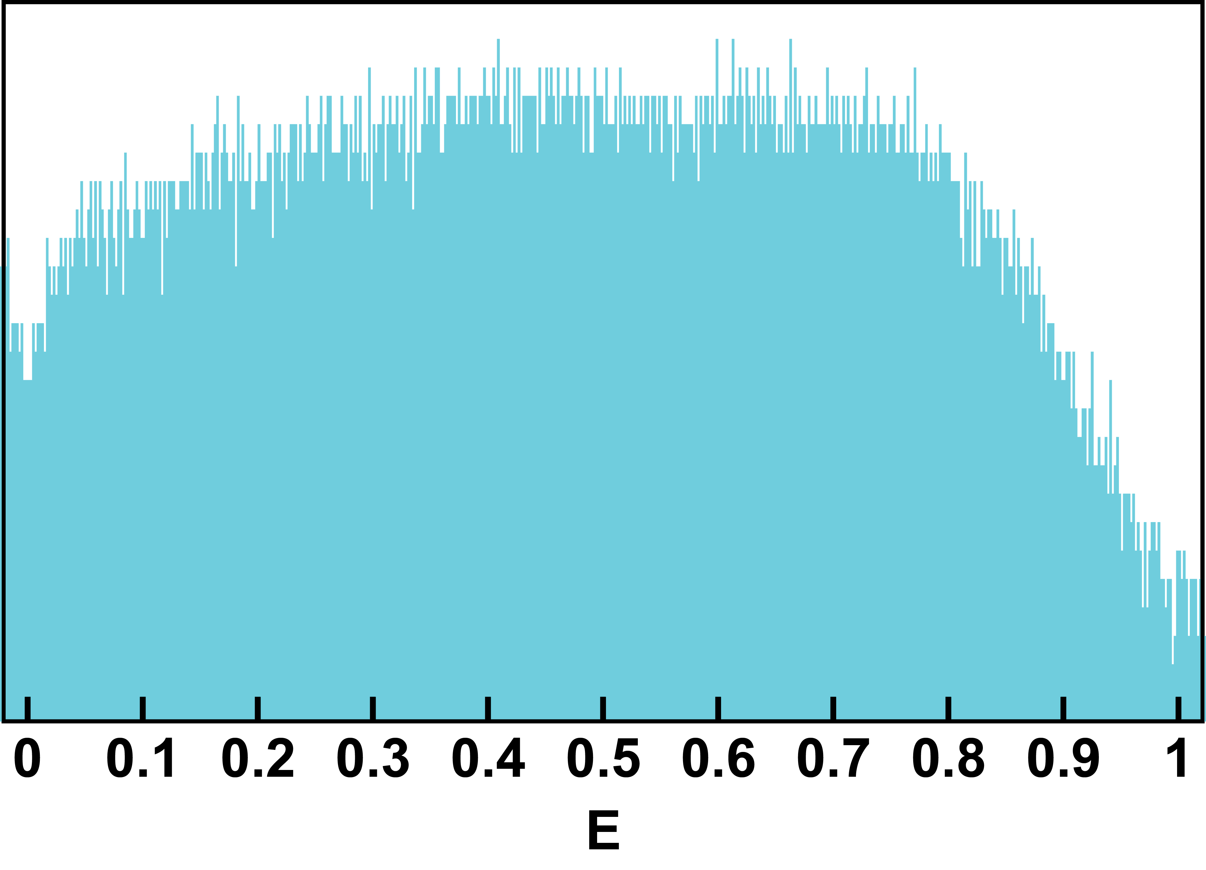
Figure S8: $k=1$, $N=34$. Box sizes $b=2,23$.

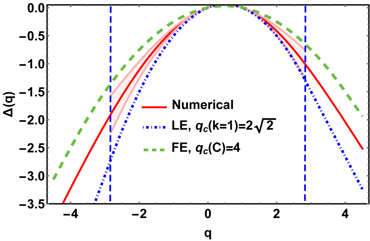
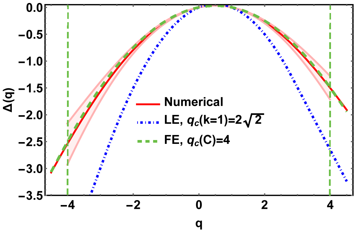
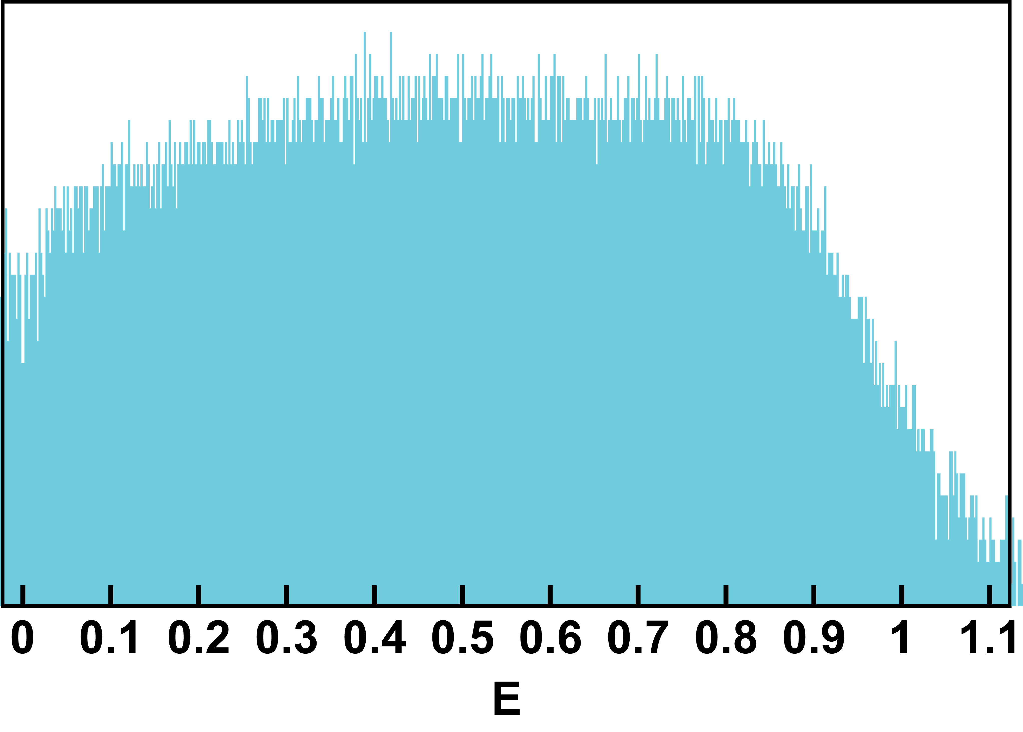
Figure S9: $k=1$, $N=36$. Box sizes $b=3,6$.

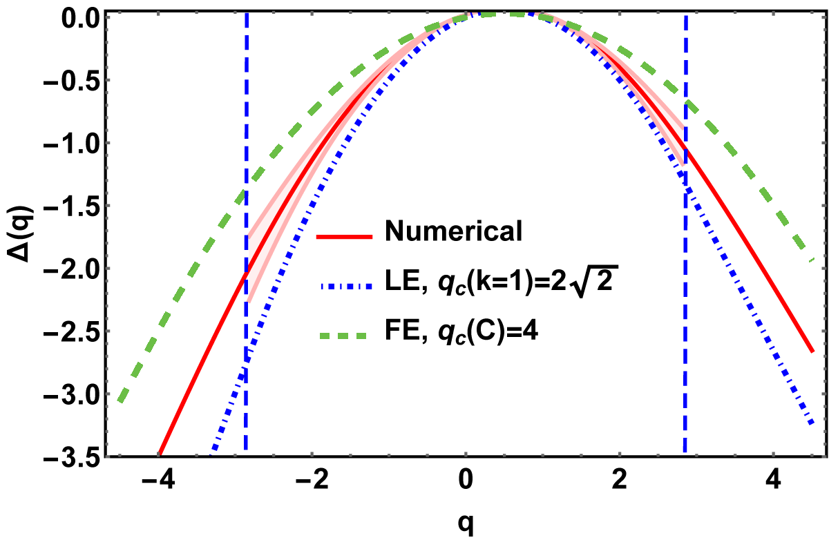
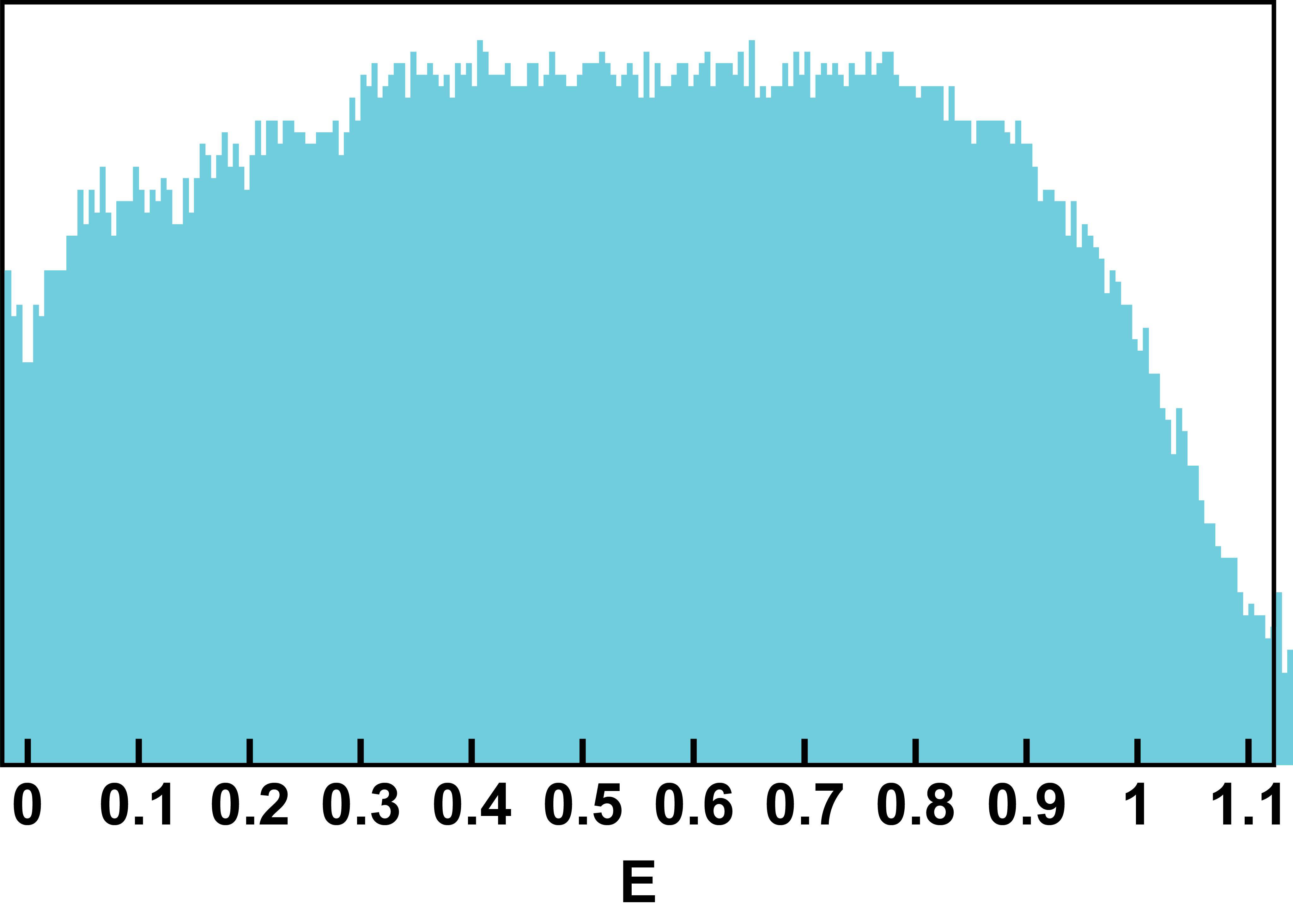
Figure S10: $k=1$, $N=38$. Box sizes $b=2,7$.

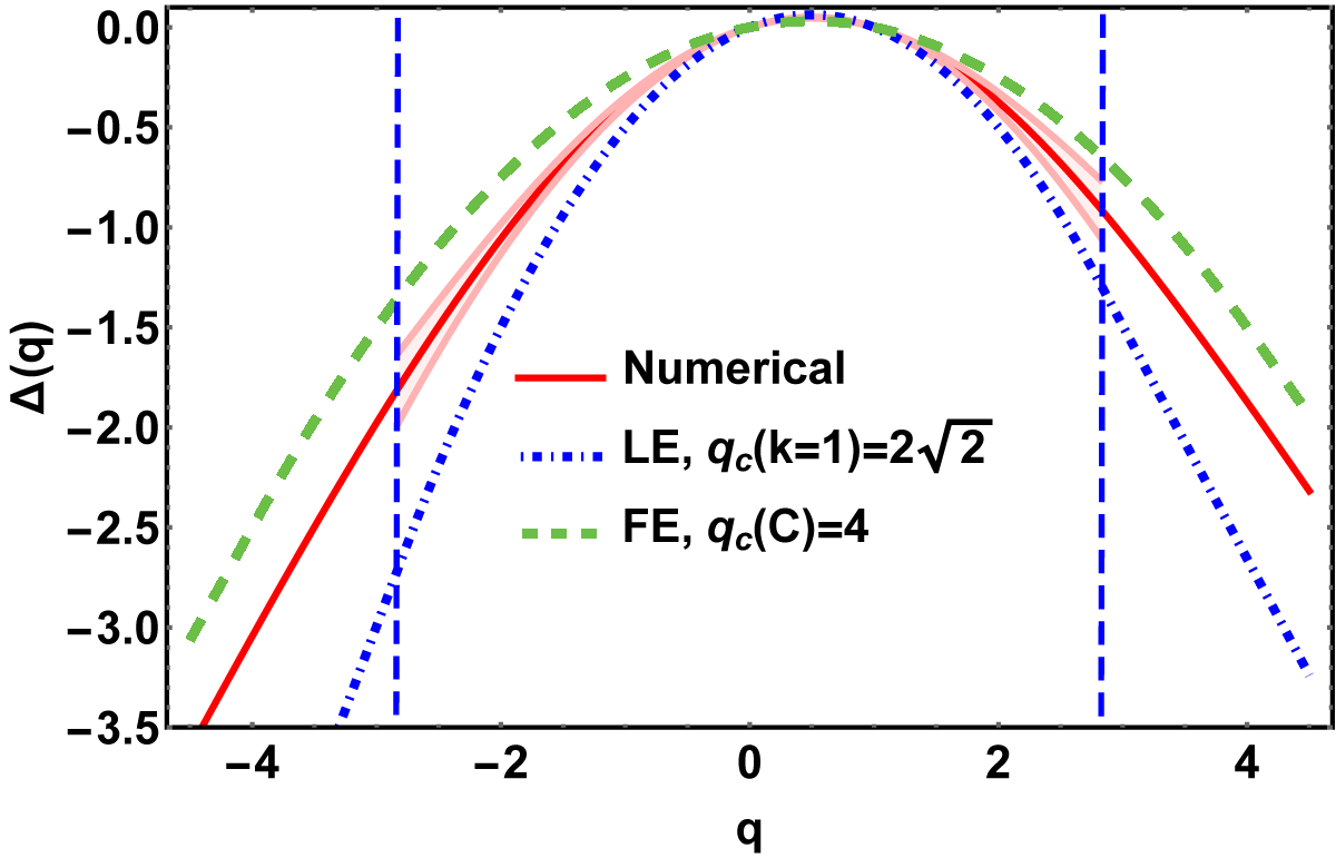
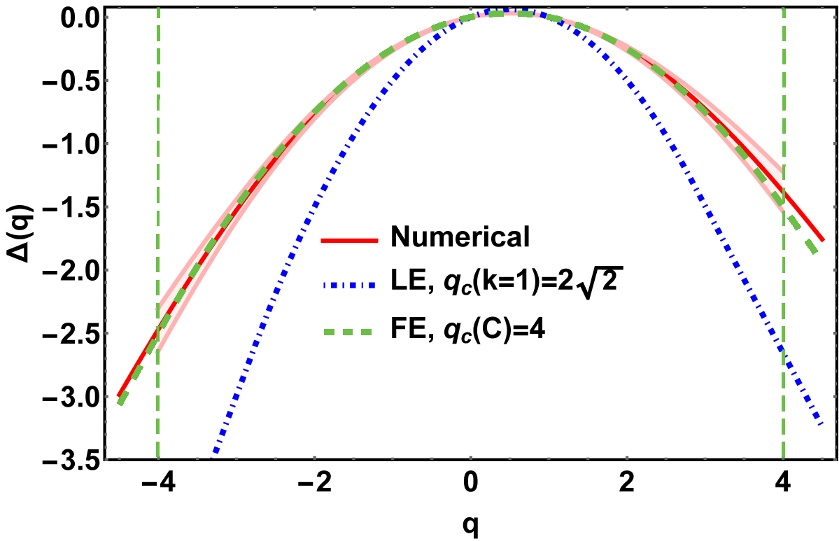
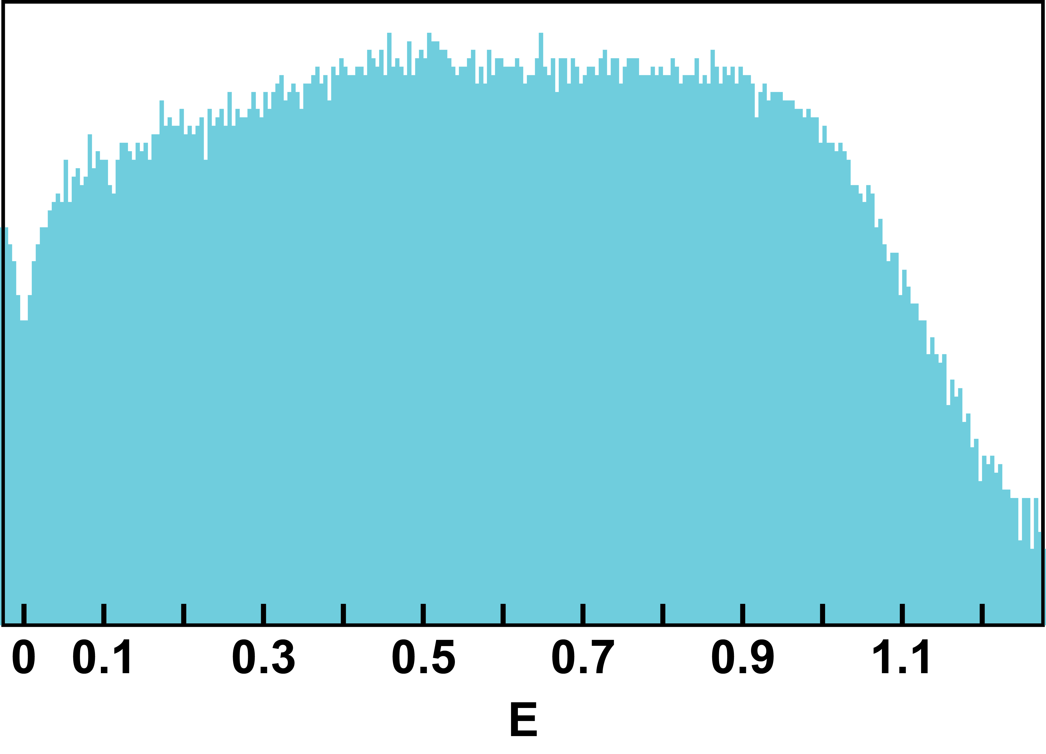
Figure S11: $k=1$, $N=42$. Box sizes $b=2,14$.

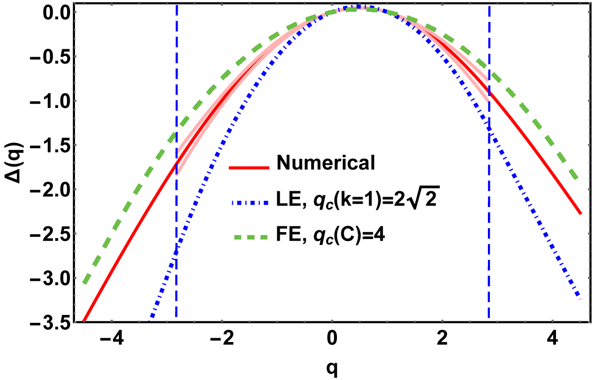
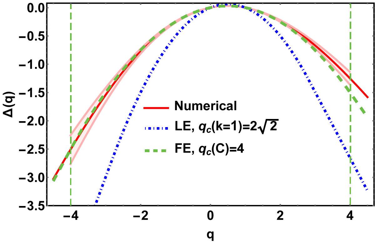
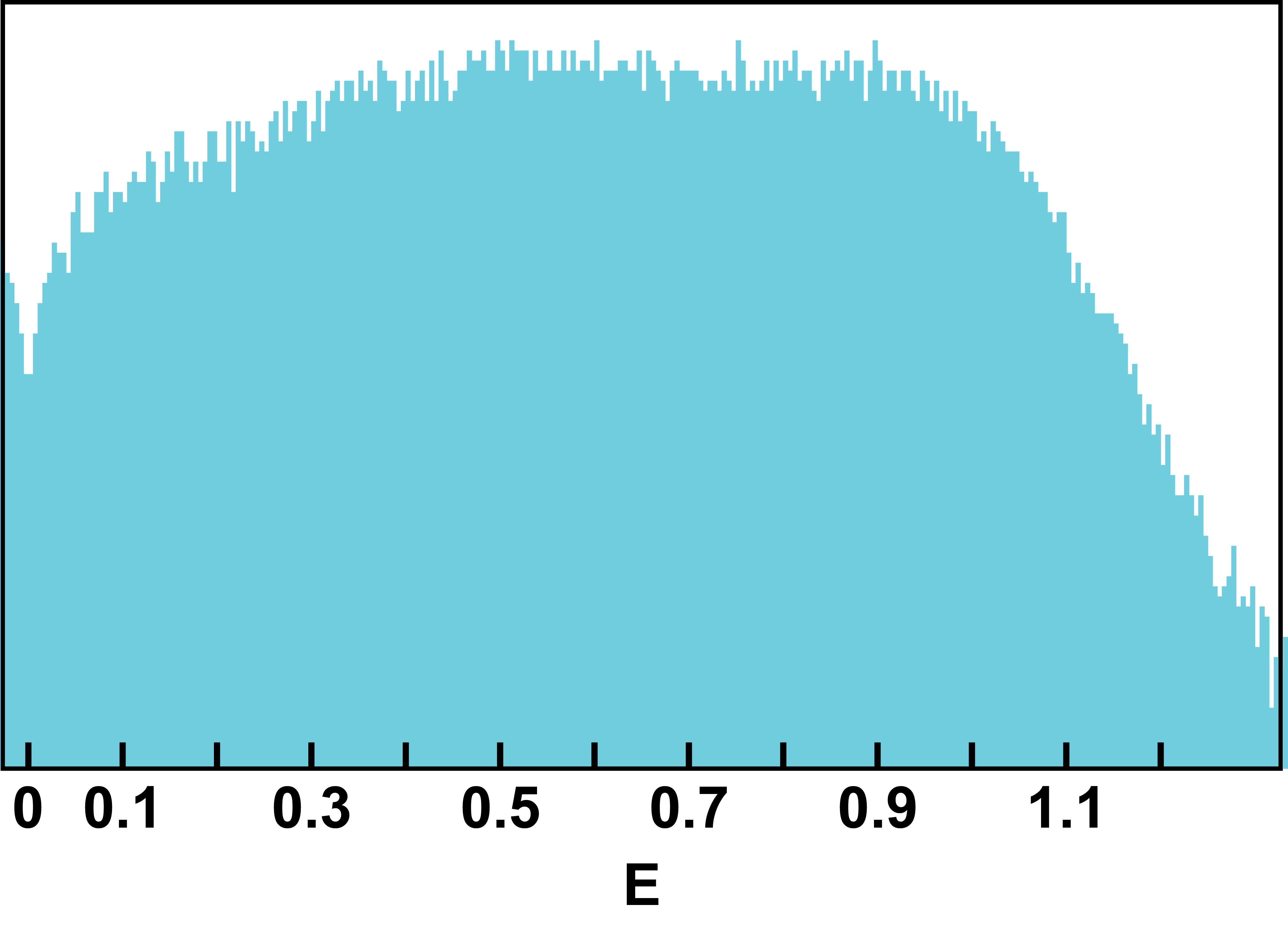
Figure S12: $k=1$, $N=44$. Box sizes $b=2,22$.

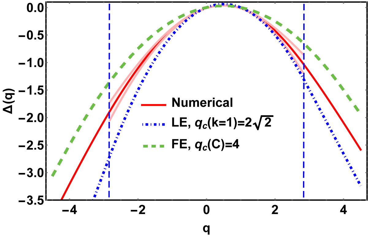
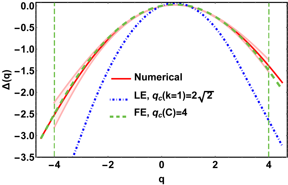
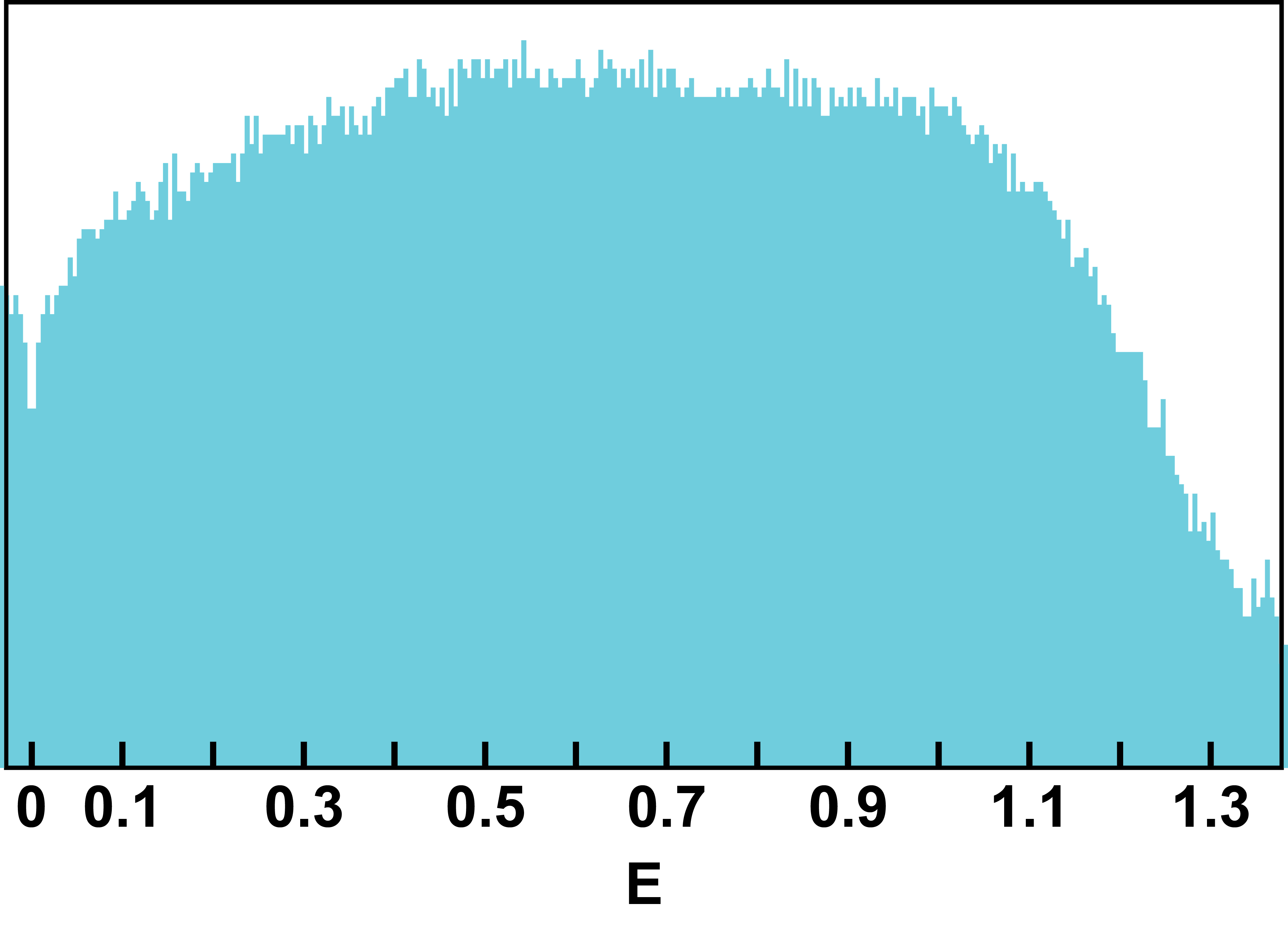
Figure S13: $k=1$, $N=46$. Box sizes $b=2,13$.

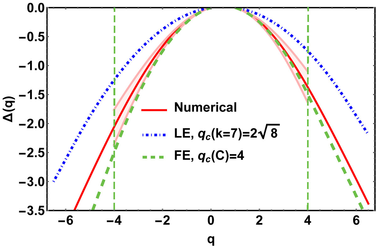
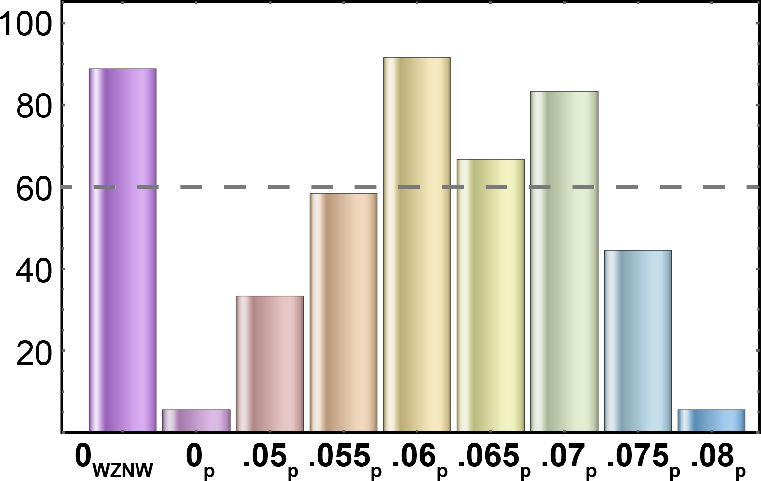
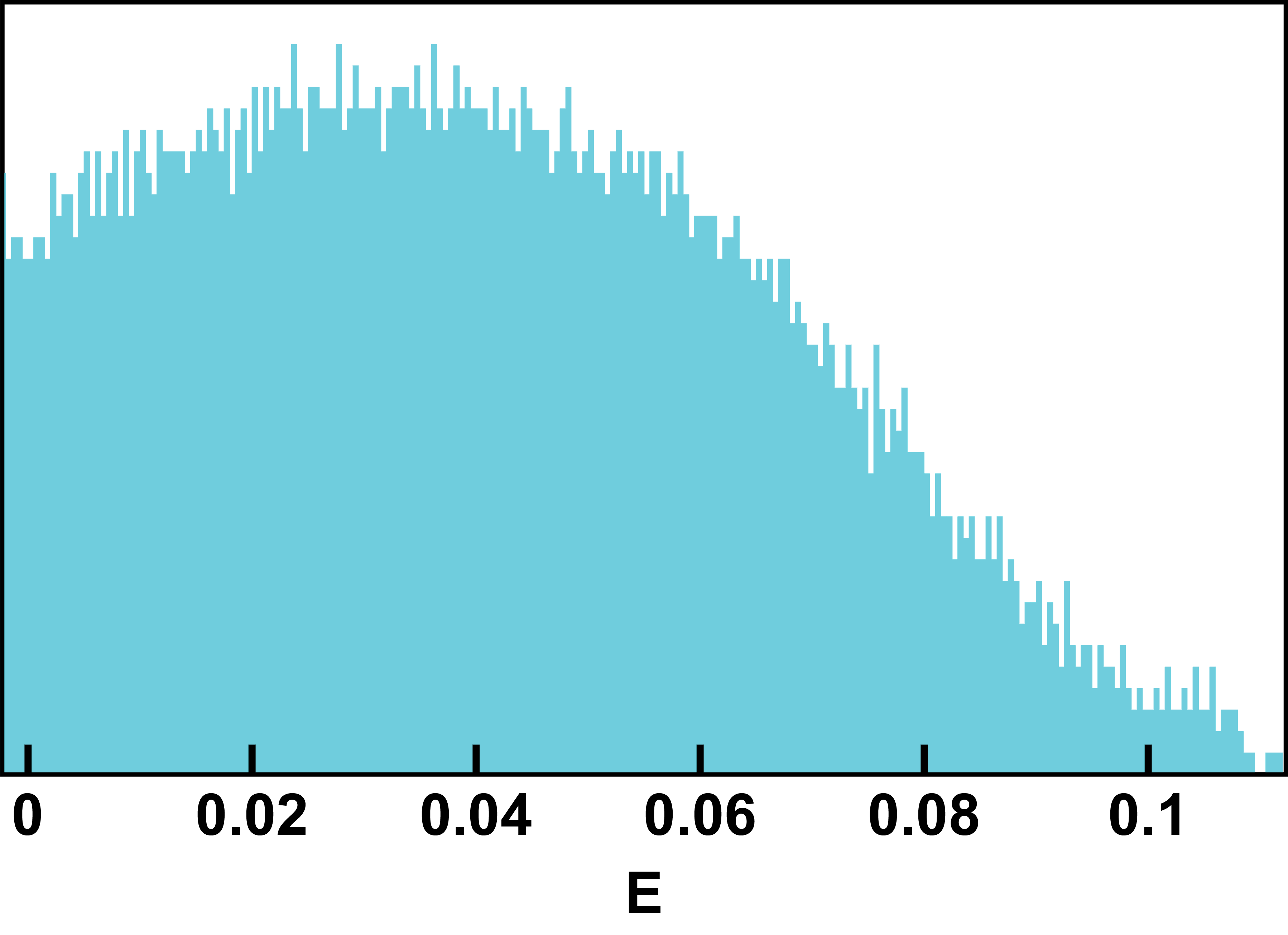
Figure S14: $k=7$, $N=24$. Box sizes $b=3,12$.

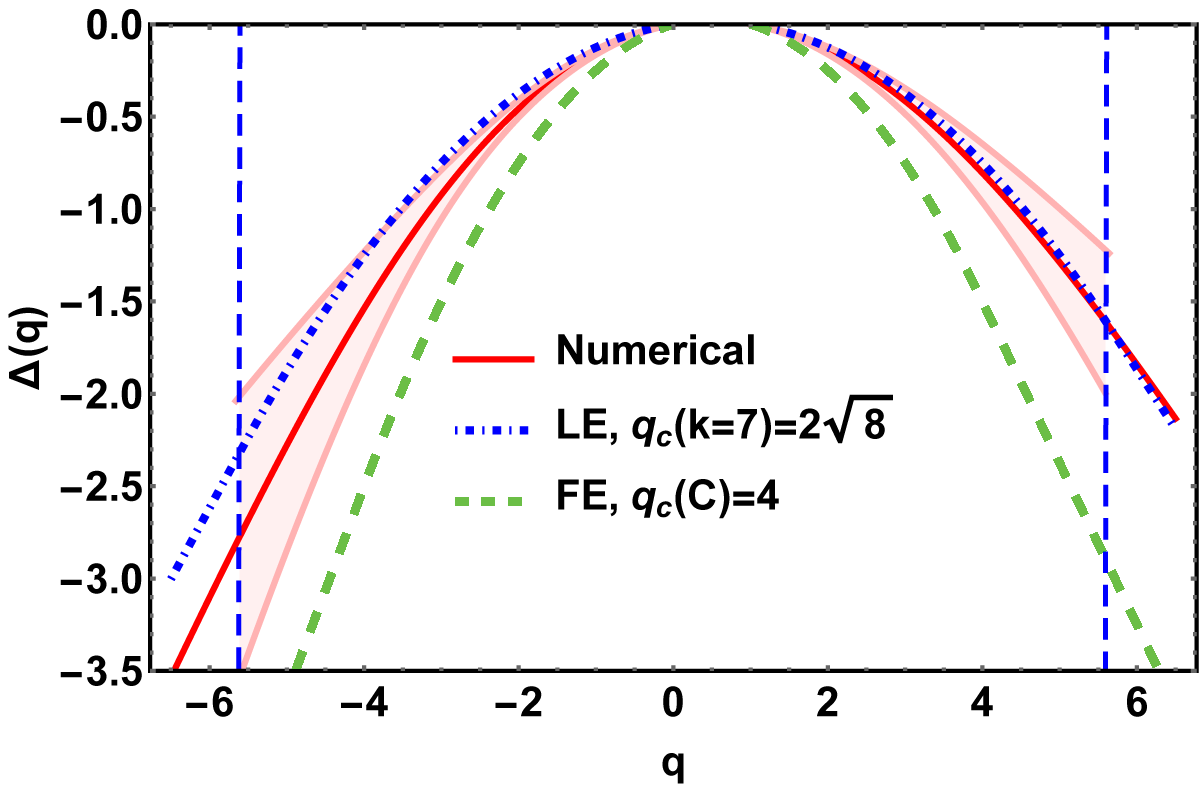
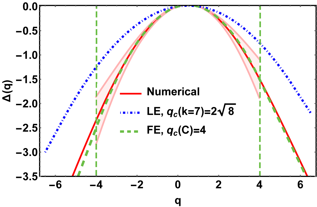
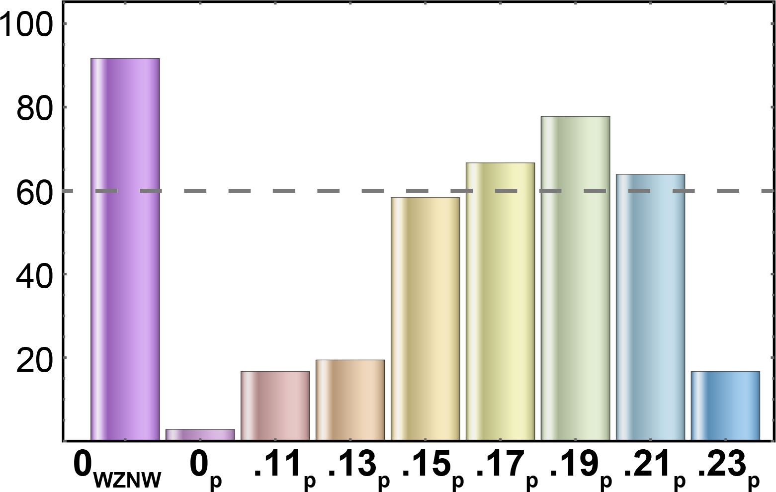
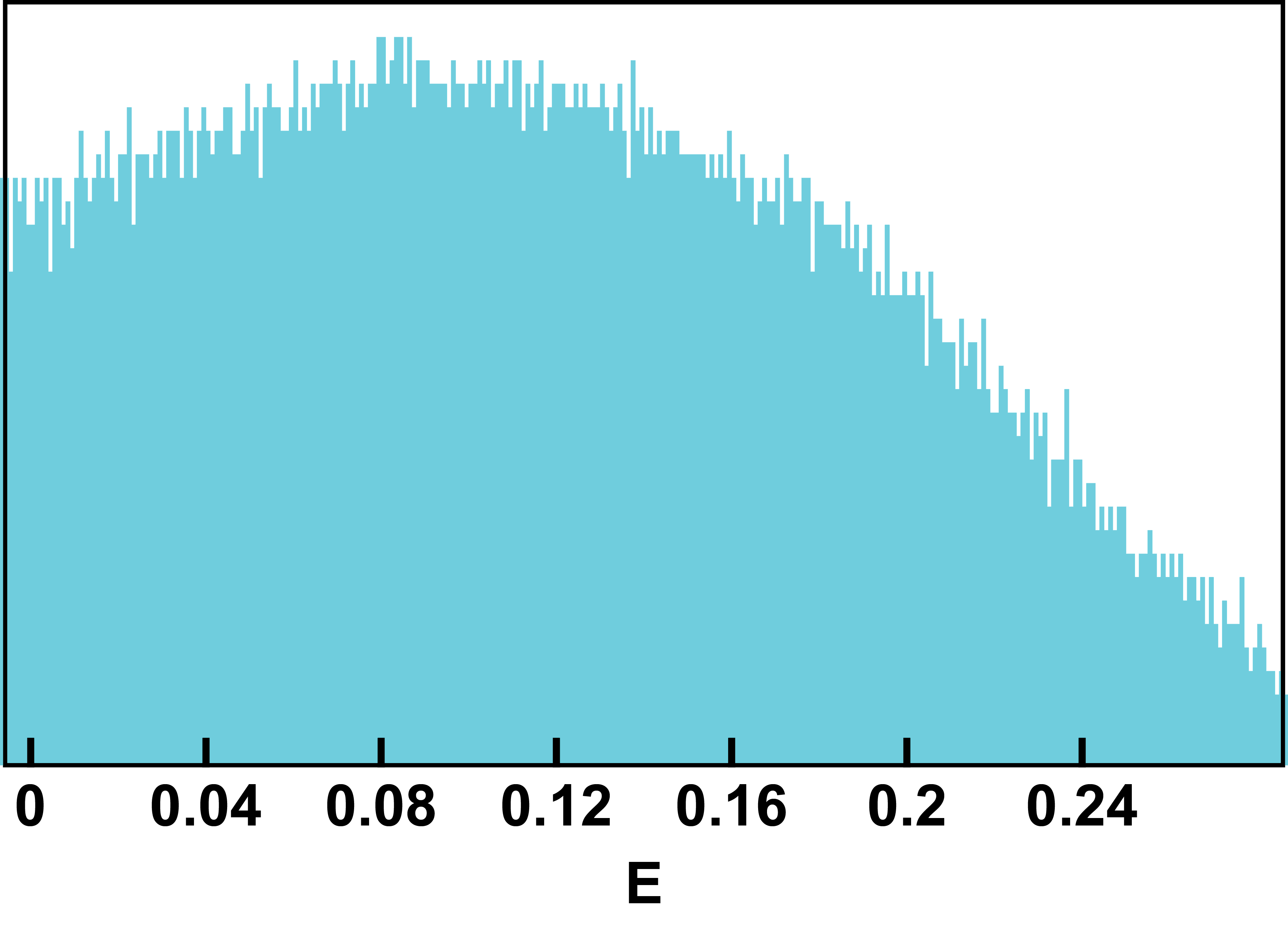
Figure S15: $k=7$, $N=28$. Box sizes $b=4,8$.

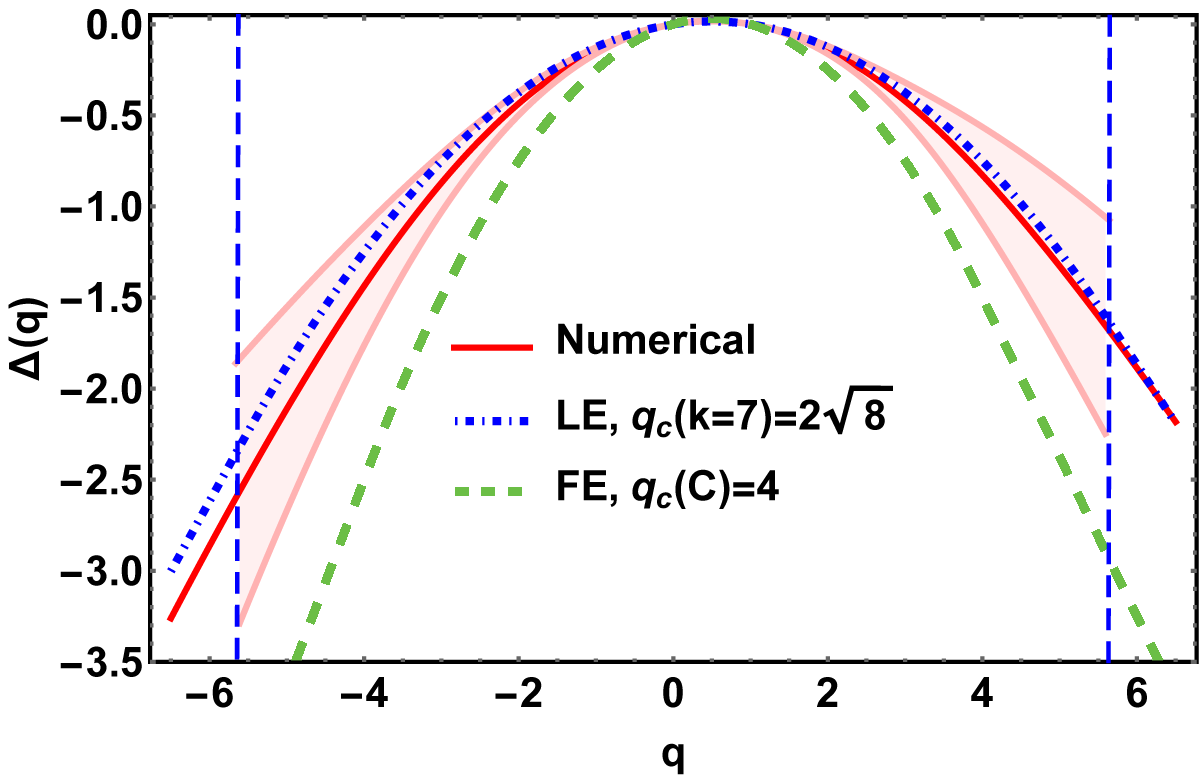
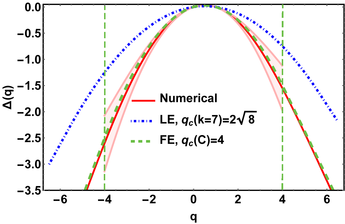
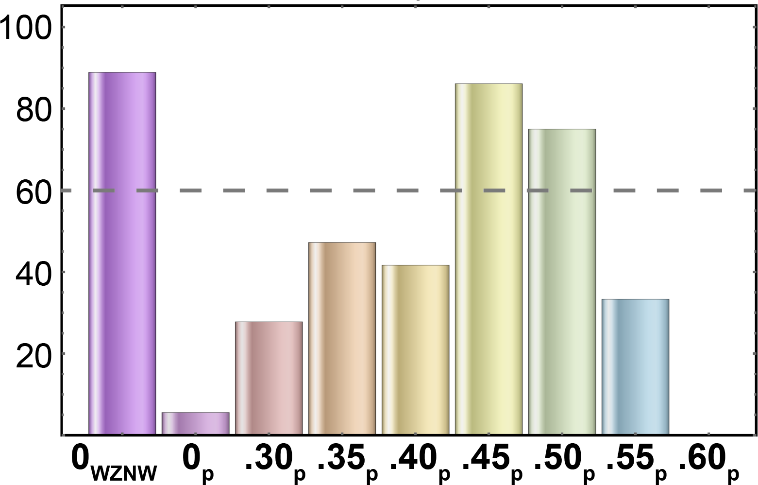
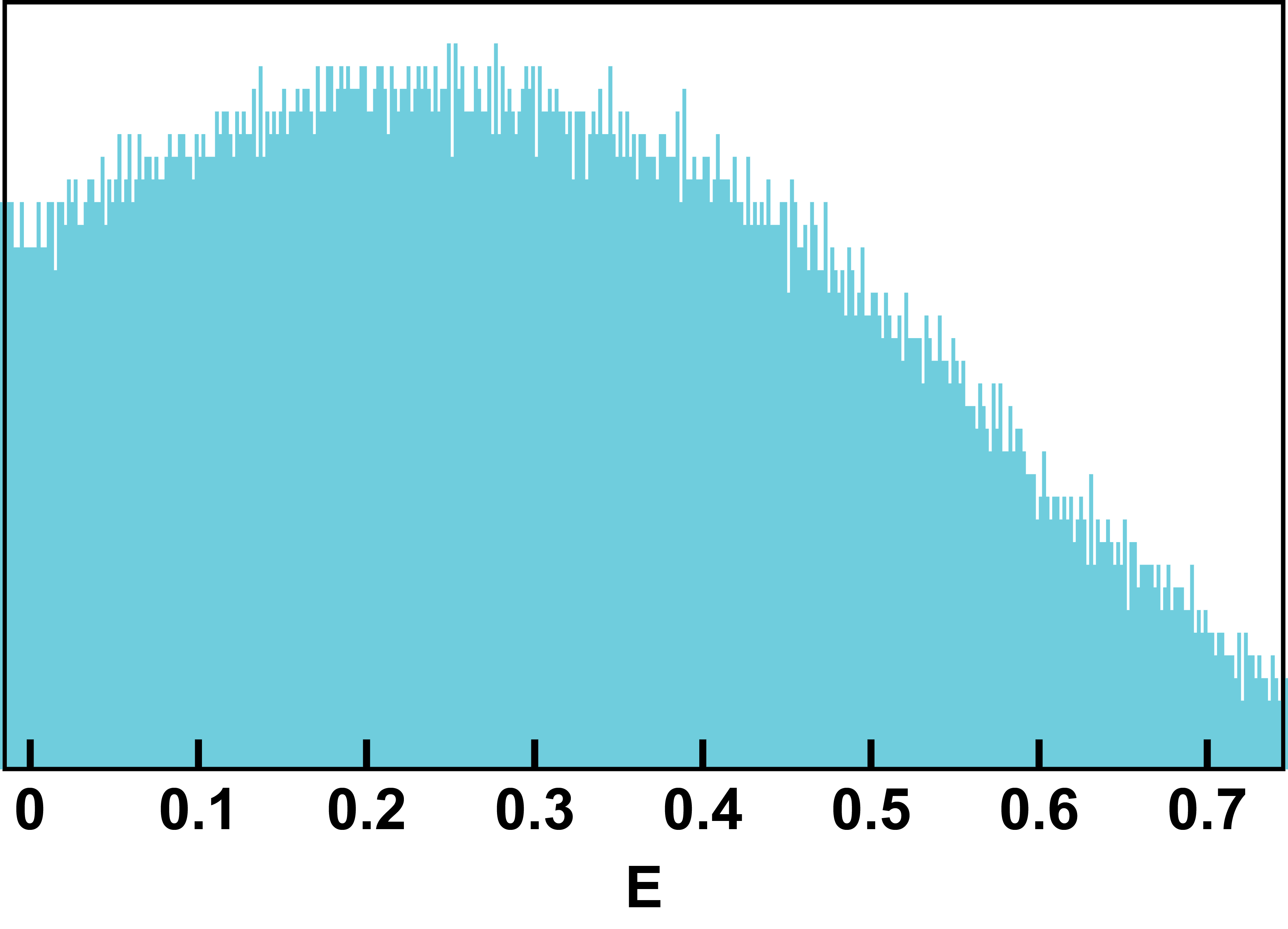
Figure S16: $k=7$, $N=32$. Box sizes $b=4,8$.

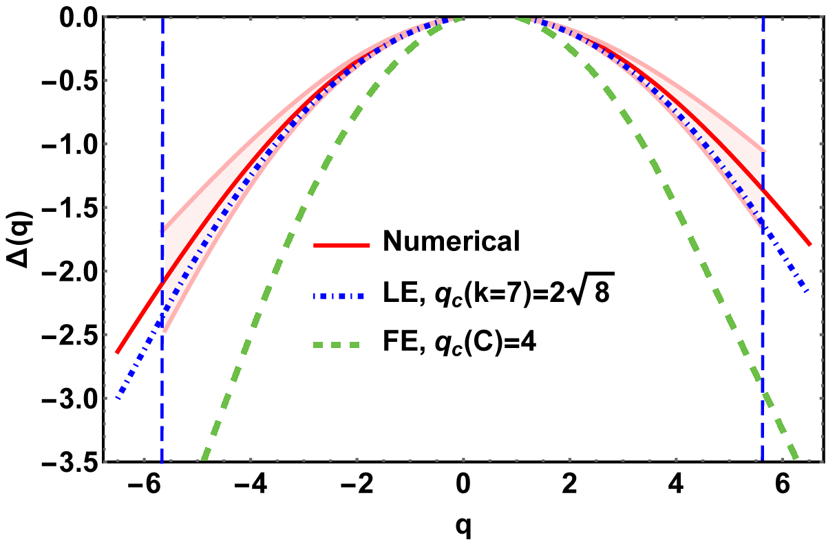
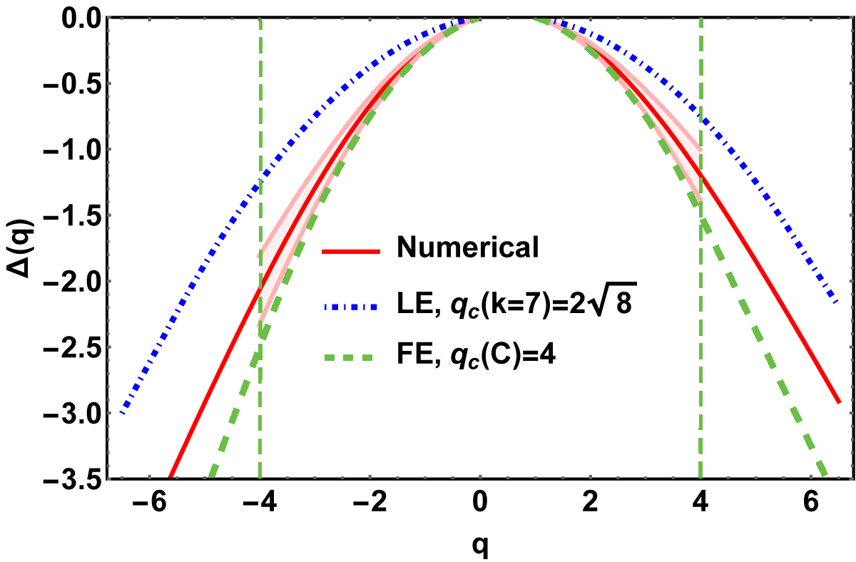
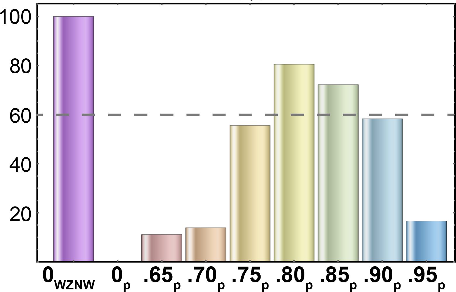
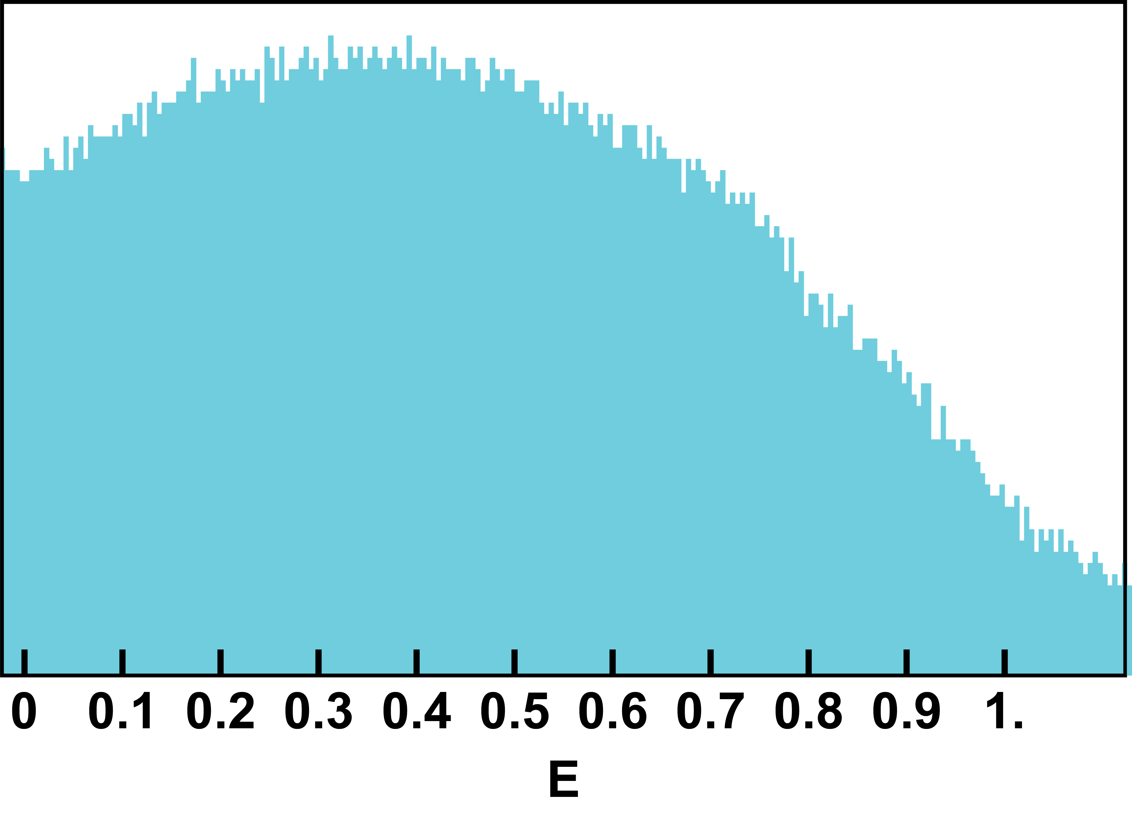
Figure S17: $k=7$, $N=34$. Box sizes $b=4,17$.

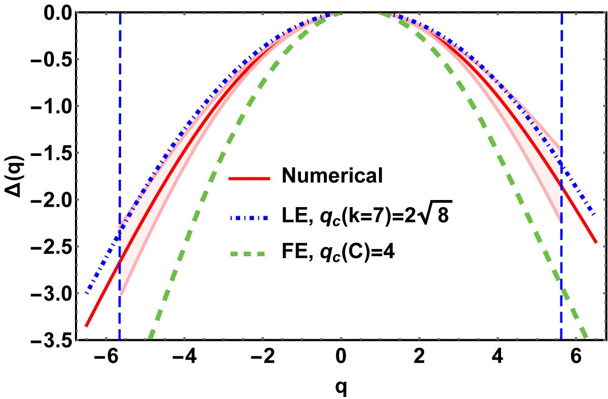
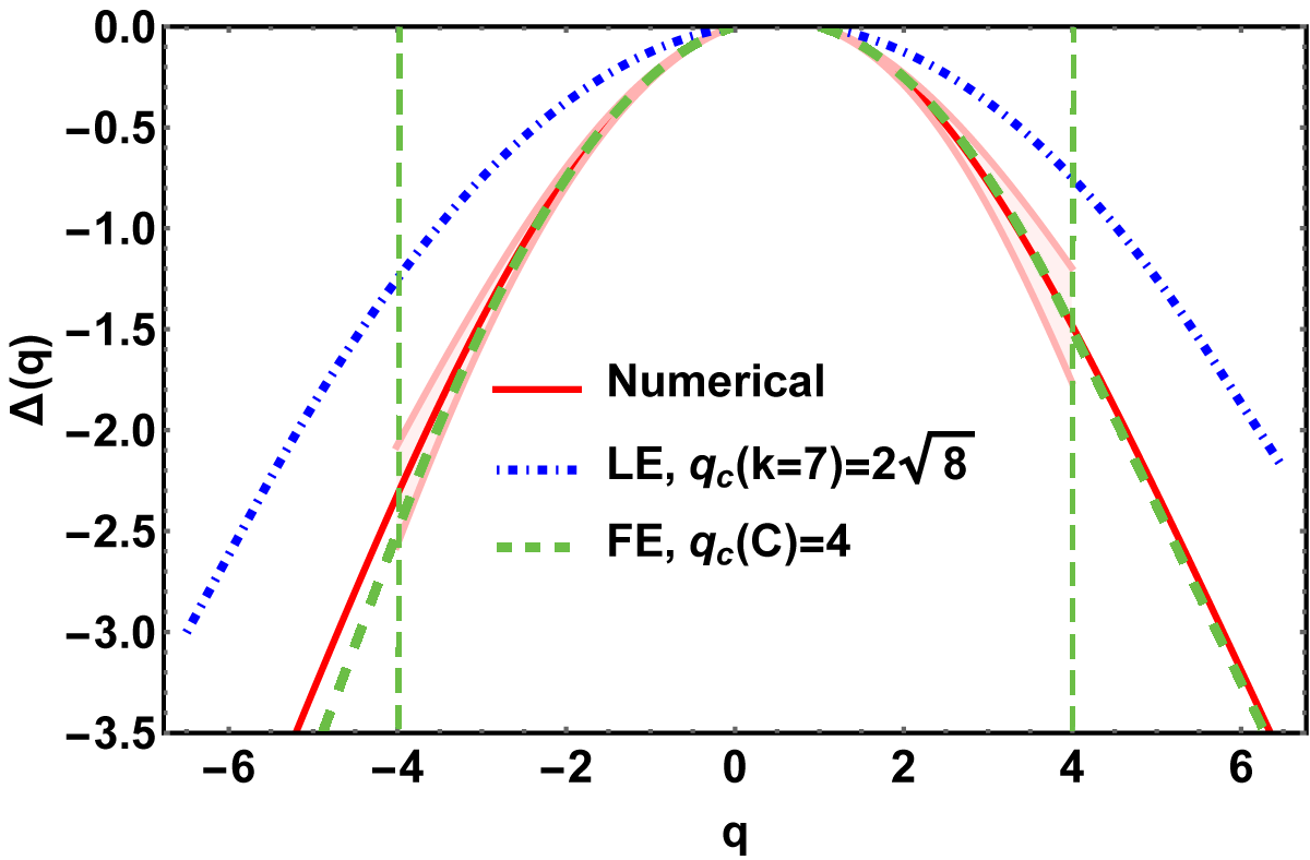
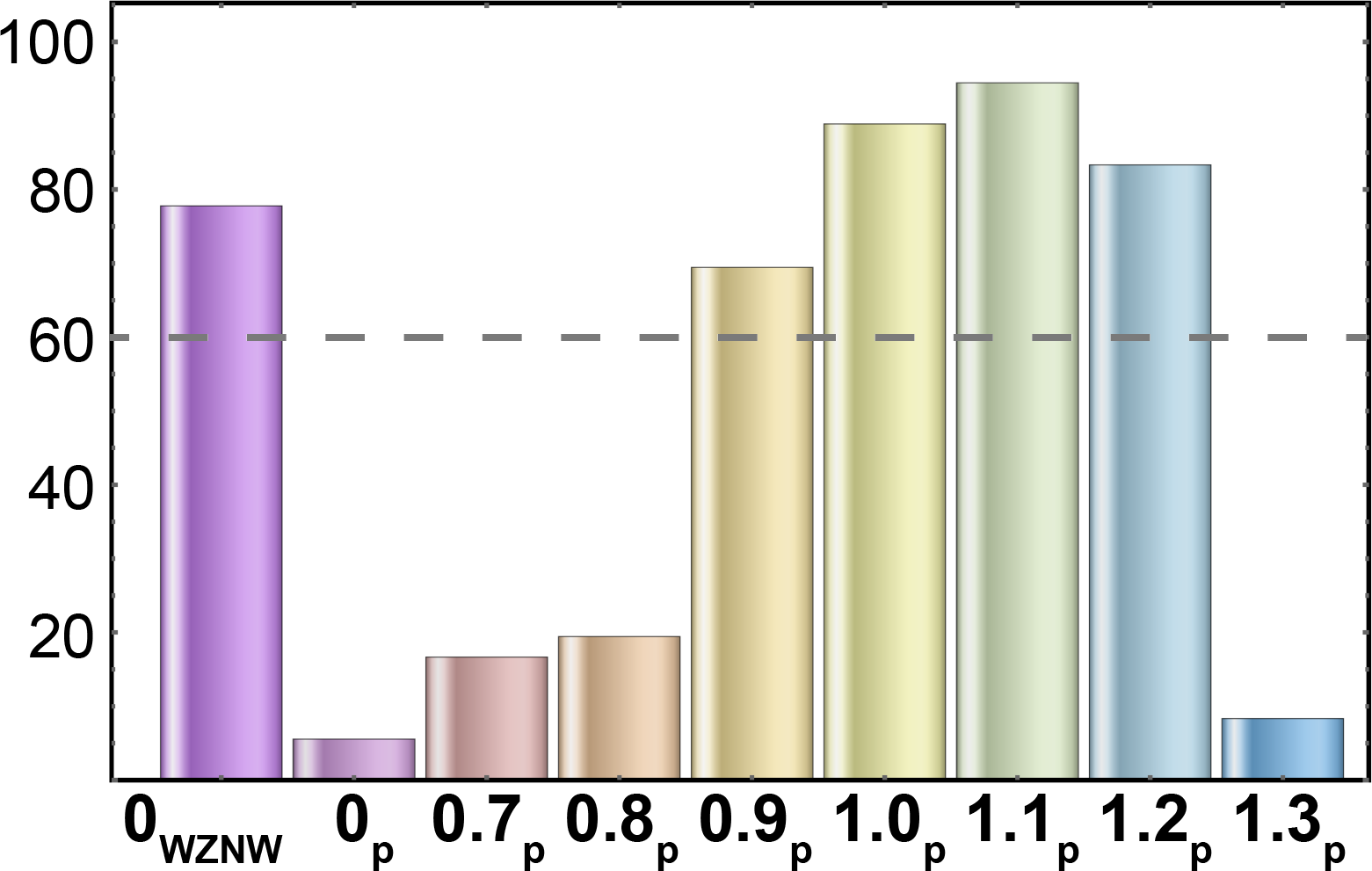
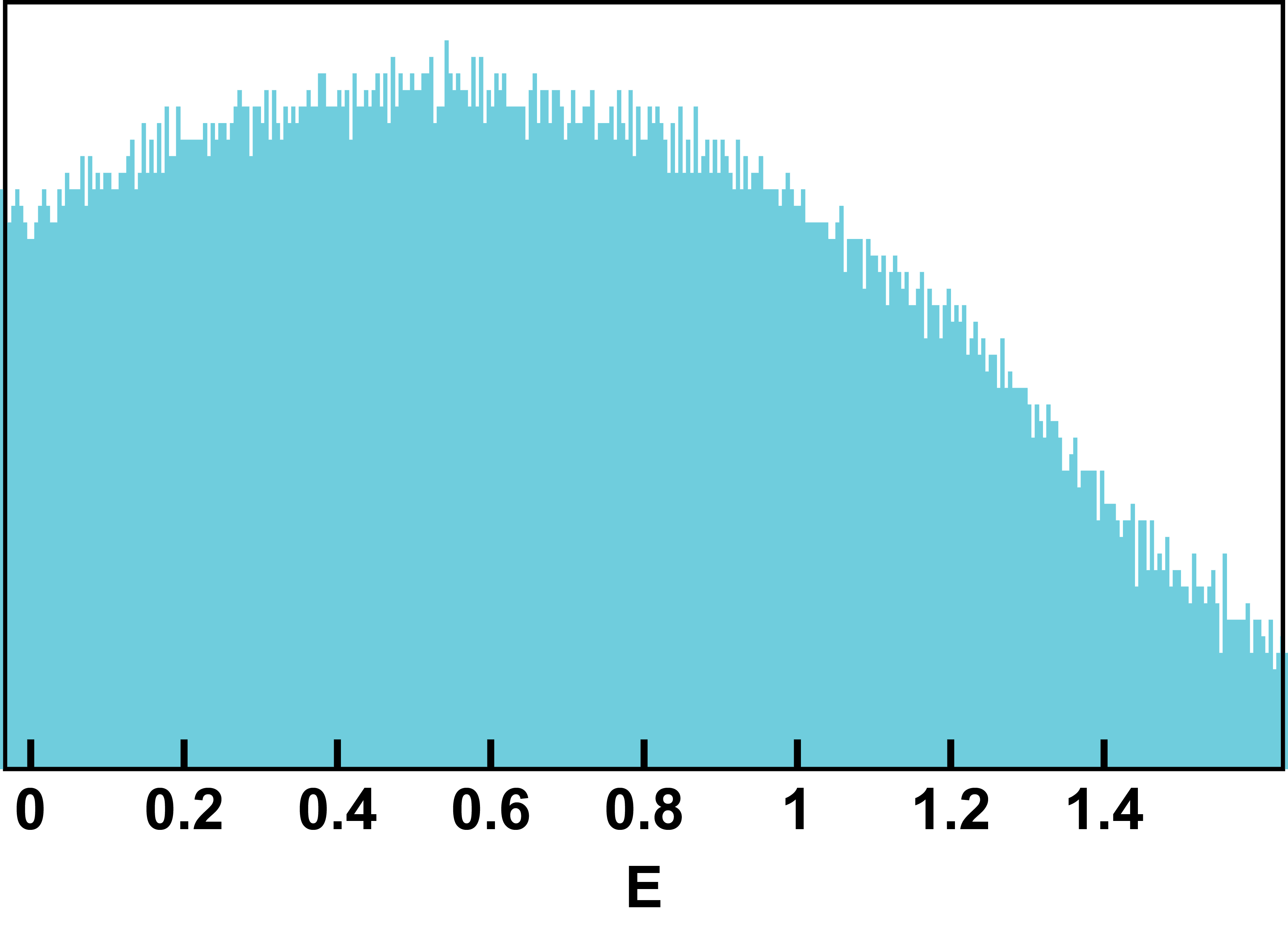
Figure S18: $k=7$, $N=36$. Box sizes $b=3,12$.

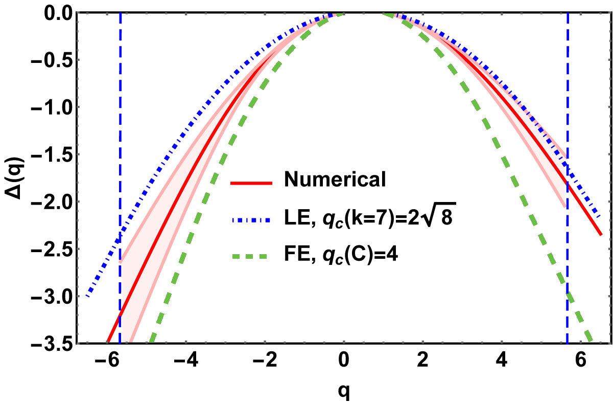
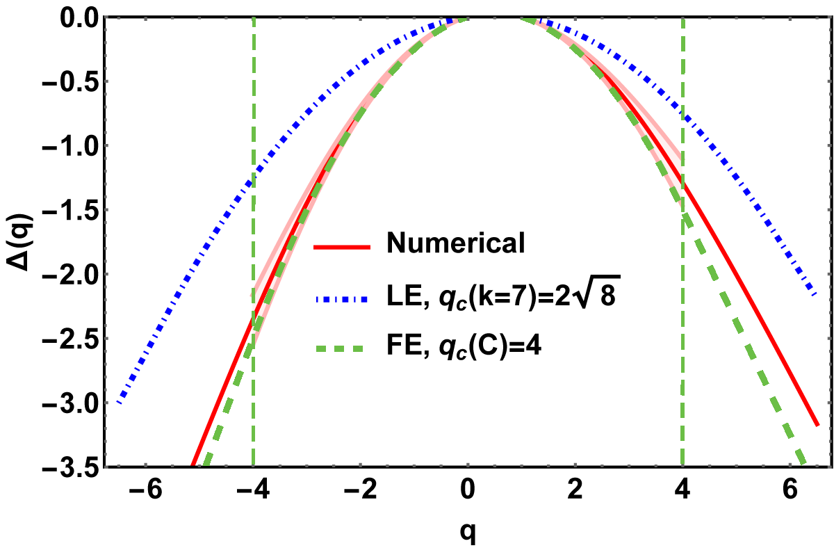
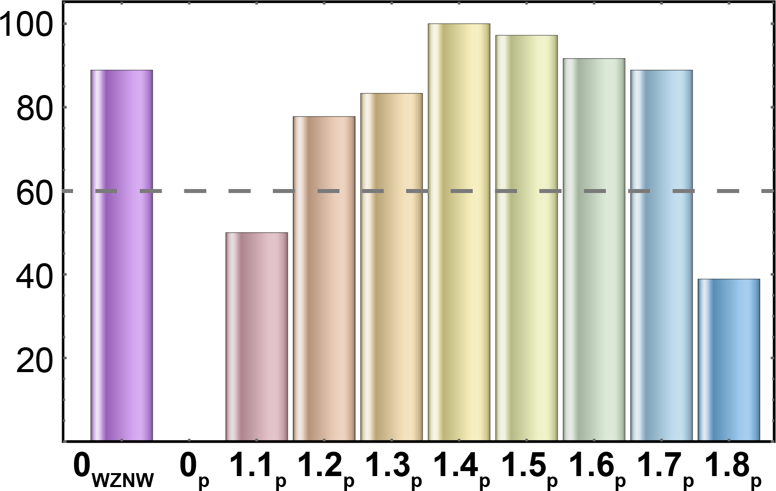
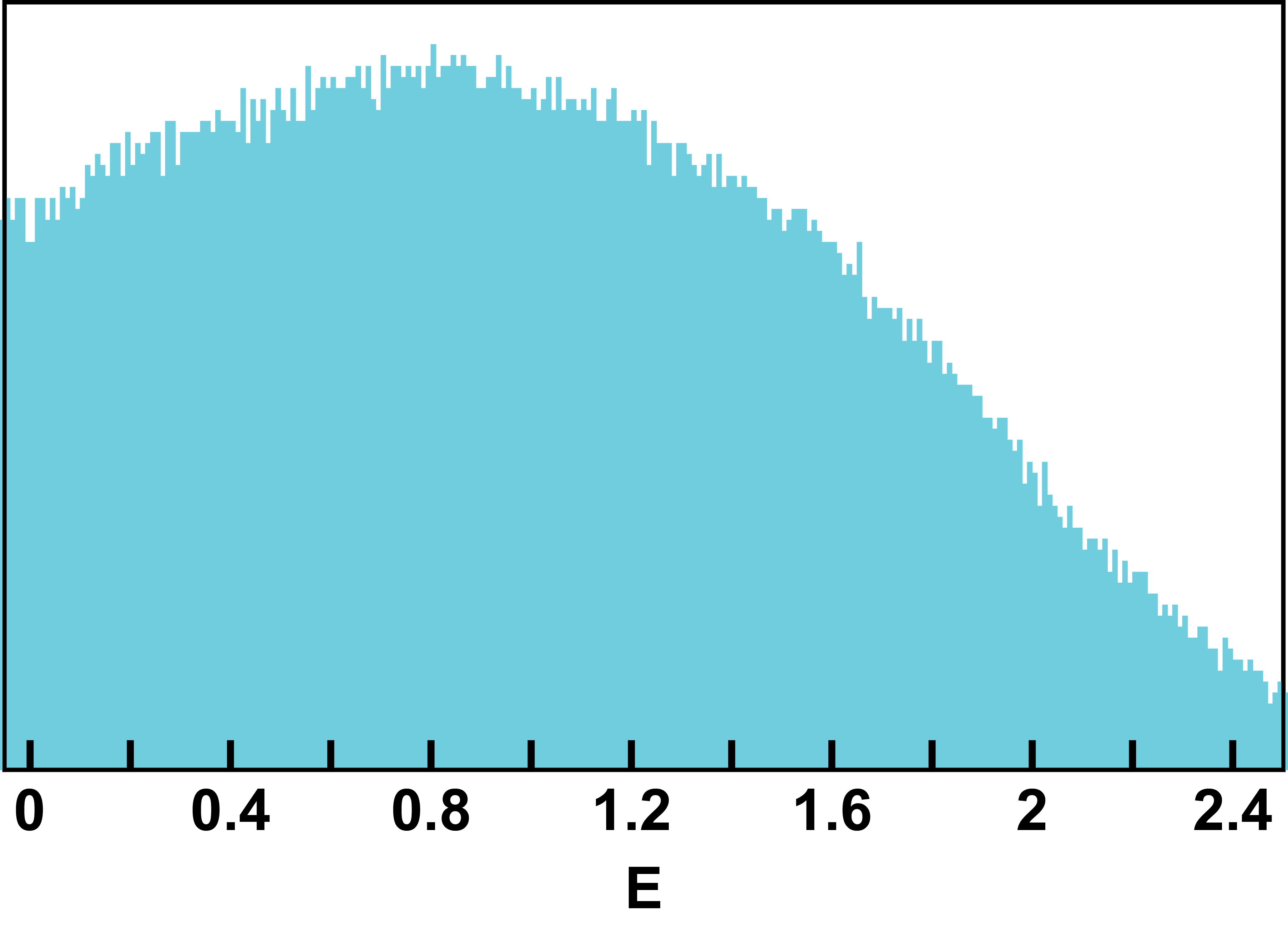
Figure S19: $k=7$, $N=38$. Box sizes $b=2,19$.

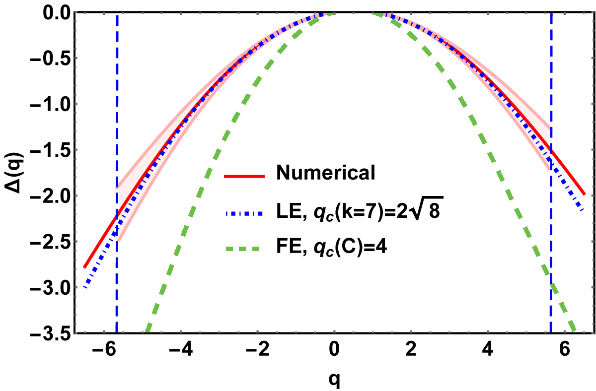
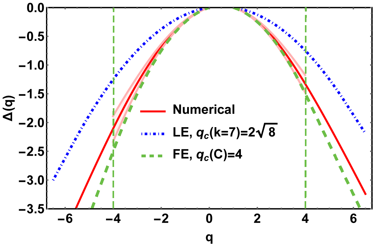
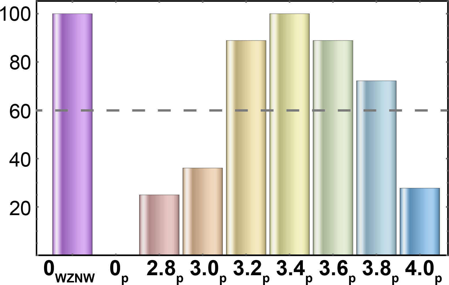
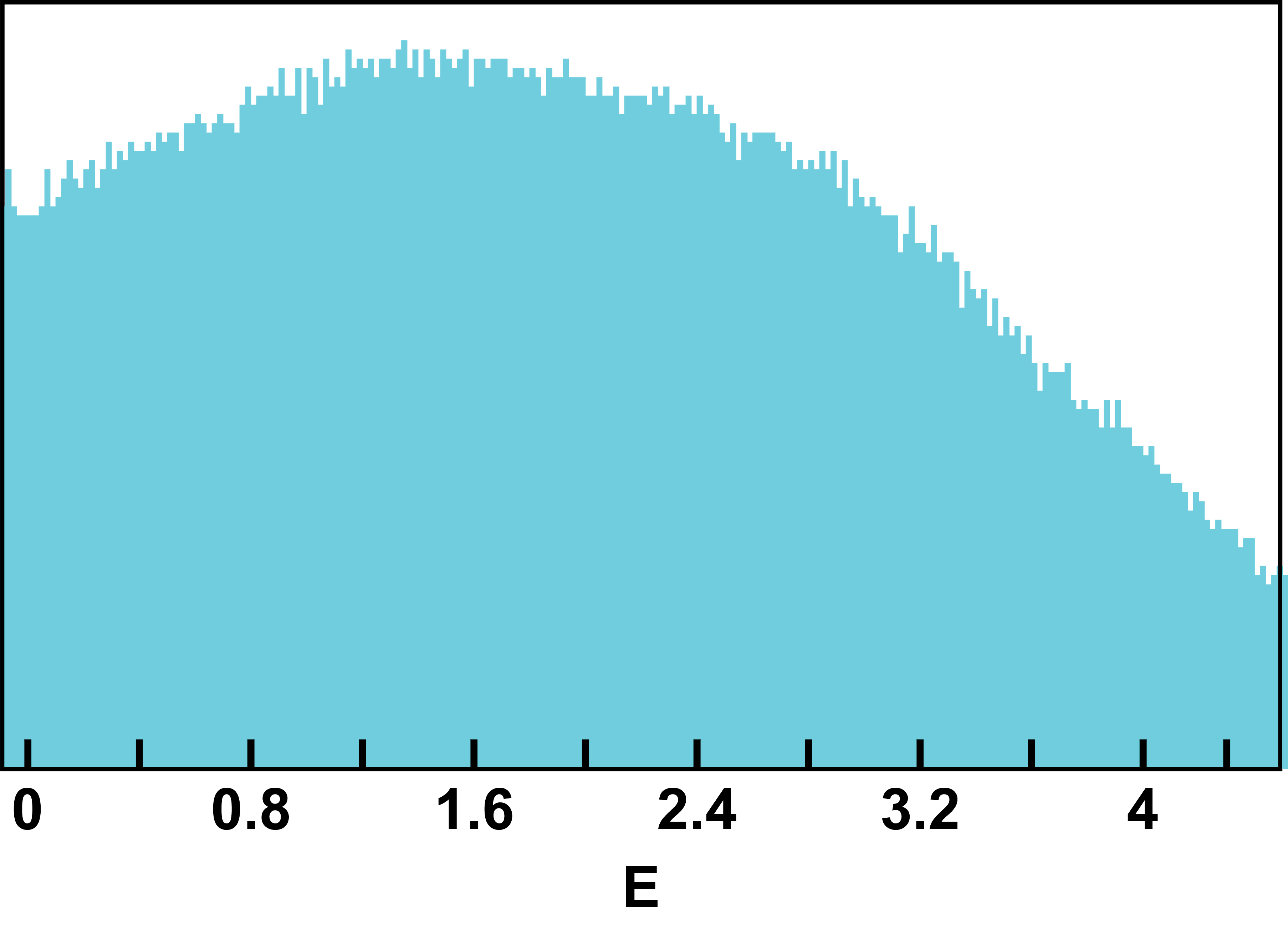
Figure S20: $k=7$, $N=42$. Box sizes $b=3,21$.

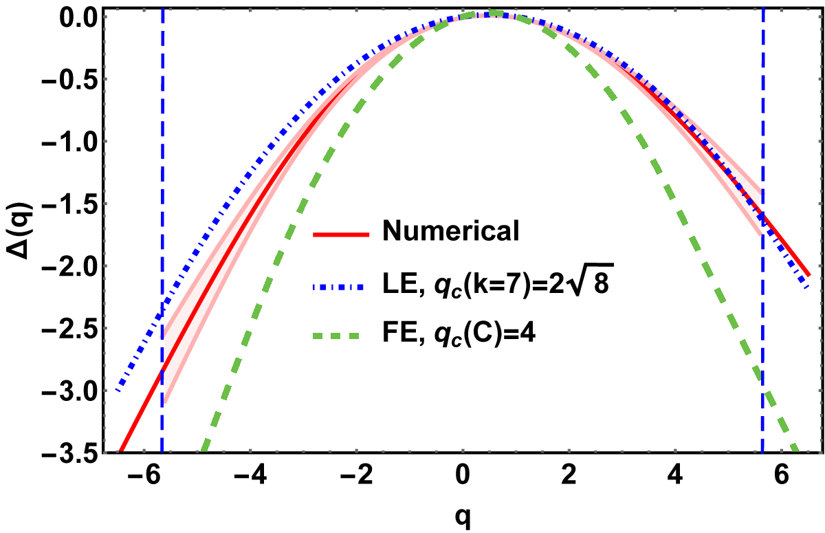
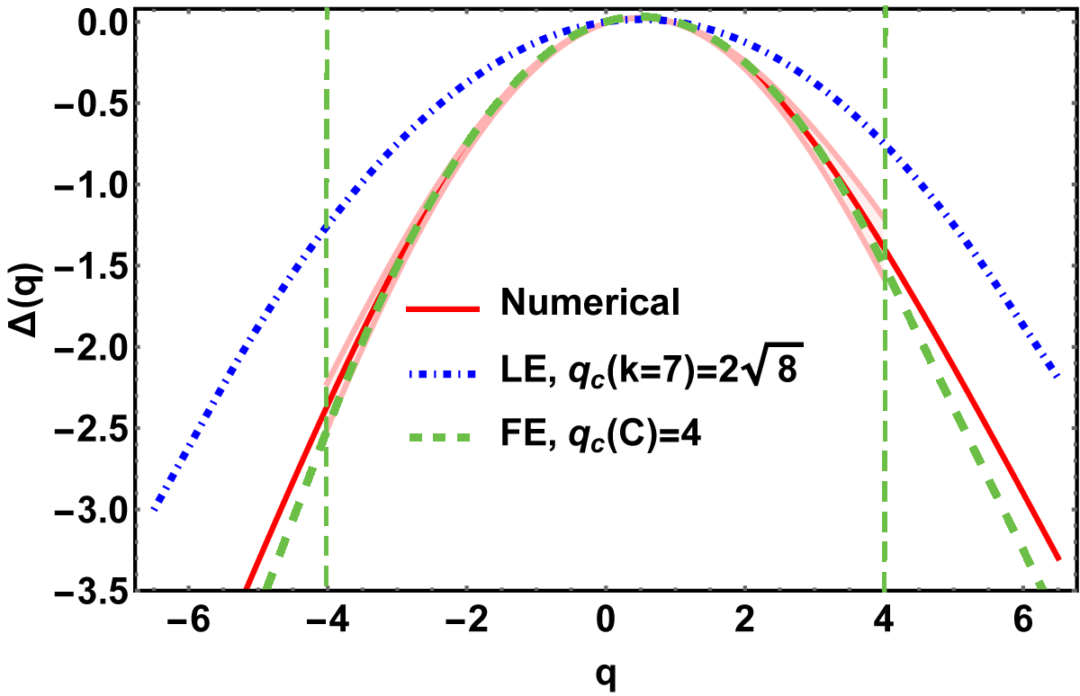
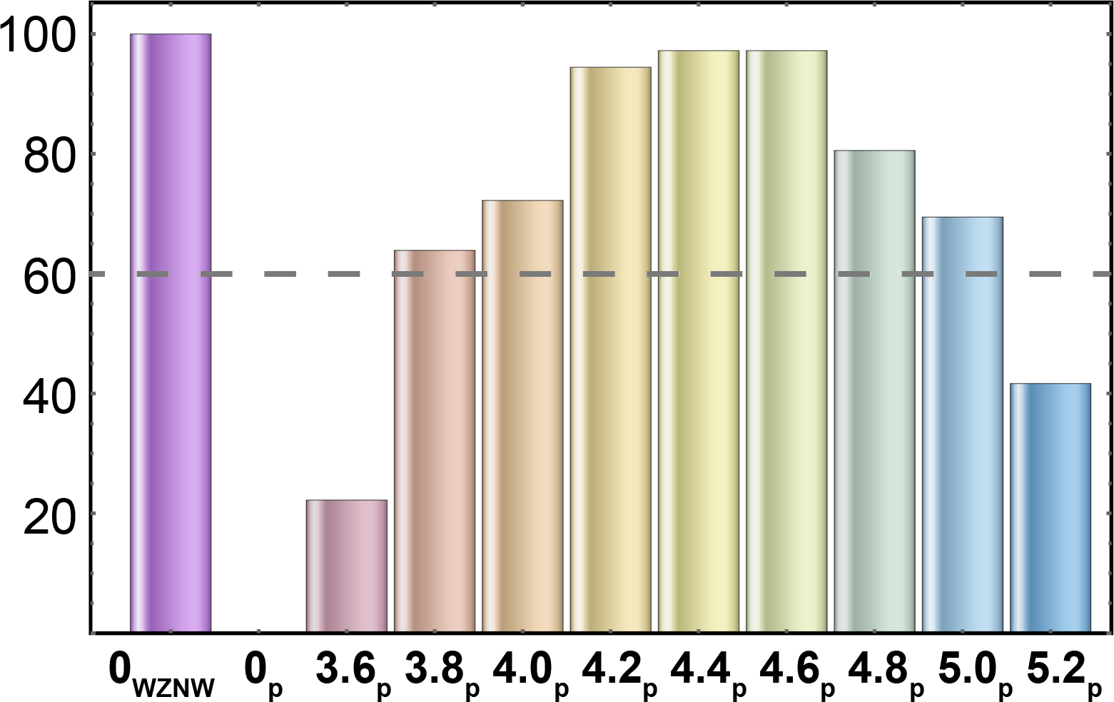
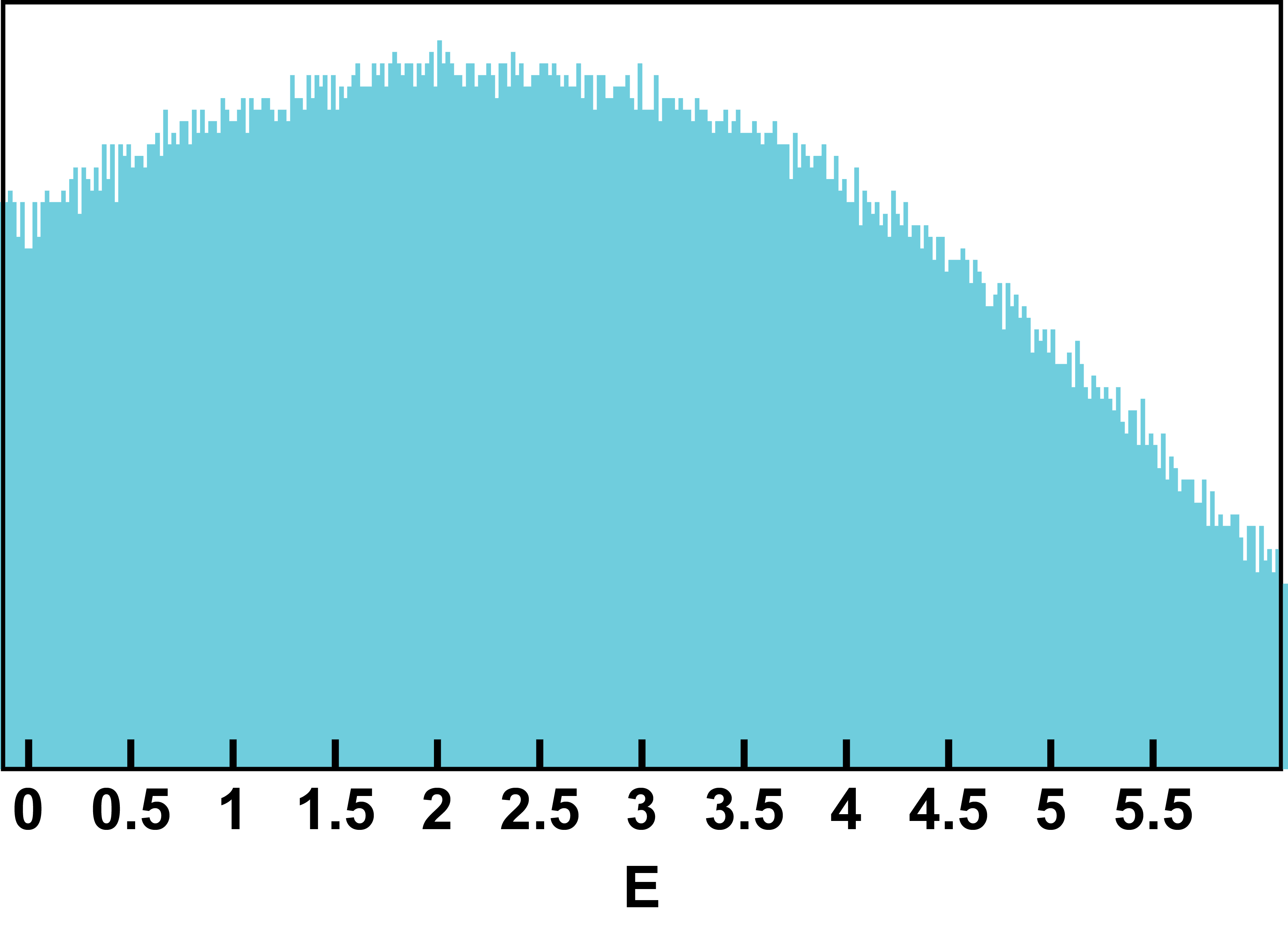
Figure S21: $k=7$, $N=44$. Box sizes $b=2,29$.

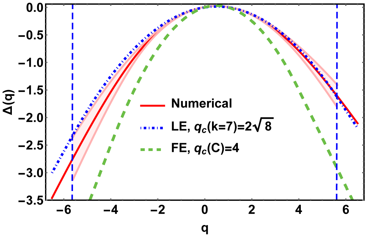
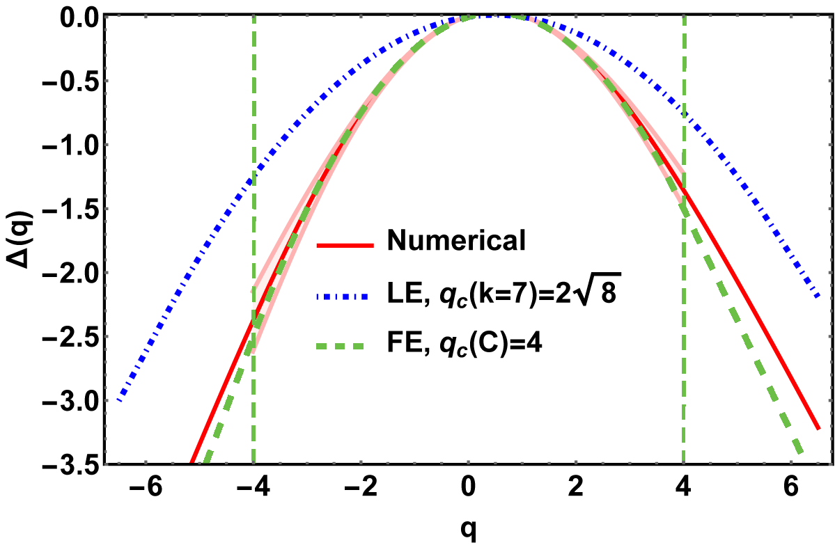
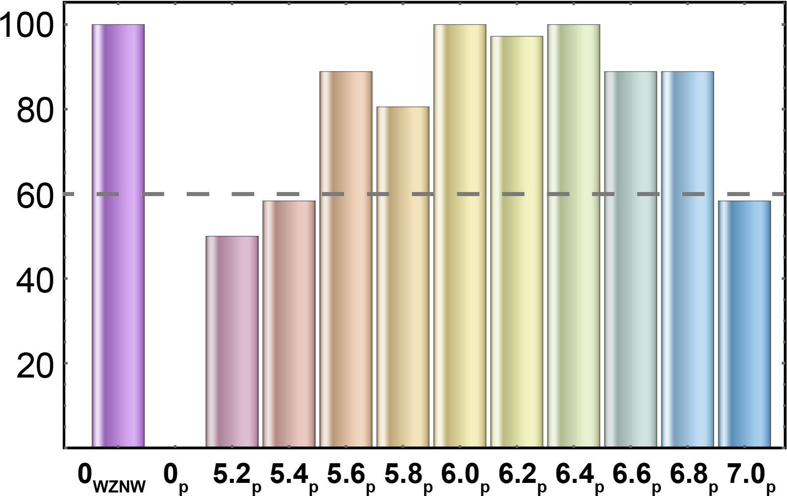
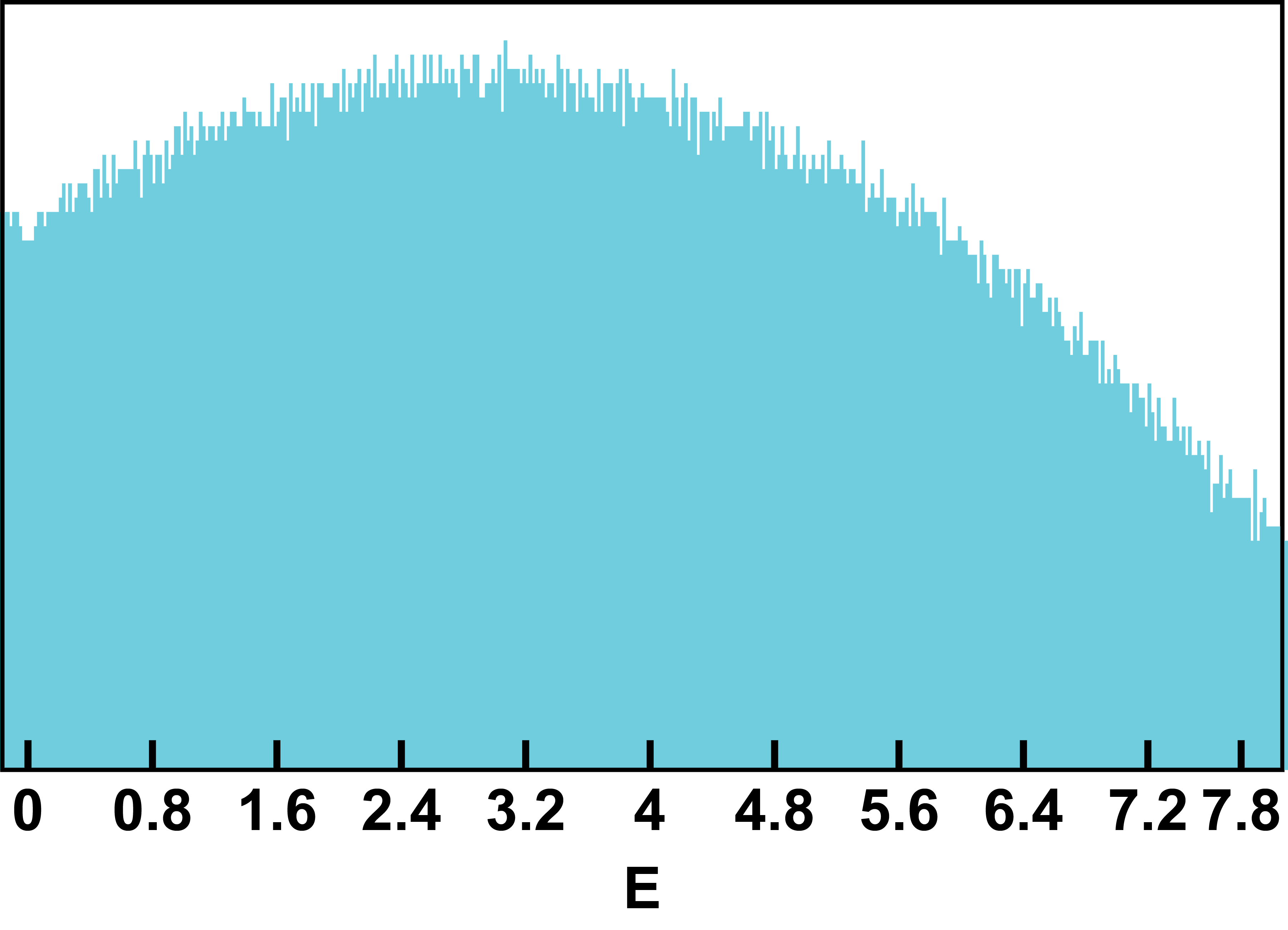
Figure S22: $k=7$, $N=46$. Box sizes $b=2,31$.

References

- (1) S. A. Trugman, Localization, percolation, and the quantum Hall effect, Phys. Rev. B 27, 7539 (1983).
- (2) B. Huckestein, Scaling theory of the integer quantum Hall effect, Rev. Mod. Phys. 67, 357 (1995).
- (3) F. Evers and A. D. Mirlin, Anderson transitions, Rev. Mod. Phys. 80, 1355 (2008).
- (4) V. Kagalovsky, B. Horovitz, Y. Avishai, and J. T. Chalker, Quantum Hall Plateau Transitions in Disordered Superconductors, Phys. Rev. Lett. 82, 3516 (1999).
- (5) I. A. Gruzberg, A. W. W. Ludwig, and N. Read, Exact Exponents for the Spin Quantum Hall Transition, Phys. Rev. Lett. 82, 4524 (1999).
- (6) T. Senthil, J. B. Marston, and M. P. A. Fisher, Spin quantum Hall effect in unconventional superconductors, Phys. Rev. B 60, 4245 (1999).
- (7) J. Cardy, Linking Numbers for Self-Avoiding Loops and Percolation: Application to the Spin Quantum Hall Transition, Phys. Rev. Lett. 84, 3507 (2000).
- (8) E. J. Beamond, J. Cardy, and J. T. Chalker, Quantum and classical localization, the spin quantum Hall effect, and generalizations, Phys. Rev. B 65, 214301 (2002).
- (9) F. Evers, A. Mildenberger, and A. D. Mirlin, Multifractality at the spin quantum Hall transition, Phys. Rev. B 67, 041303R (2003).
- (10) A. D. Mirlin, F. Evers, and A. Mildenberger, Wavefunction statistics and multifractality at the spin quantum Hall transition, J. Phys. A 36, 3255 (2003).
- (11) For a review, see e.g. J. Cardy, Quantum Network Models and Classical Localization Problems, in 50 Years of Anderson Localization, ed. E. Abrahams (World Scientific, Singapore, 2010).
- (12) A. W. W. Ludwig, M. P. A. Fisher, R. Shankar, G. Grinstein, Integer quantum Hall transition: An alternative approach and exact results, Phys. Rev. B, 50, 7526 (1994).
- (13) P. M. Ostrovsky, I. V. Gornyi, and A. D. Mirlin, Quantum Criticality and Minimal Conductivity in Graphene with Long-Range Disorder, Phys. Rev. Lett. 98, 256801 (2007).
- (14) Y.-Z. Chou and M. S. Foster, Chalker scaling, level repulsion, and conformal invariance in critically delocalized quantum matter: Disordered topological superconductors and artificial graphene, Phys. Rev. B 89, 165136 (2014).
- (15) A. P. Schnyder, S. Ryu, A. Furusaki, and A. W. W. Ludwig, Classification of topological insulators and superconductors in three spatial dimensions, Phys. Rev. B 78, 195125 (2008).
- (16) A. Kitaev, Periodic table for topological insulators and superconductors, AIP Conf. Proc. No. 1134 (AIP, New York, 2009), p. 22.
- (17) M. S. Foster and E. A. Yuzbashyan, Interaction-Mediated Surface-State Instability in Disordered Three-Dimensional Topological Superconductors with Spin SU(2) Symmetry, Phys. Rev. Lett. 109, 246801 (2012).
- (18) M. S. Foster, H.-Y. Xie, and Y.-Z. Chou, Topological protection, disorder, and interactions: Survival at the surface of 3D topological superconductors, Phys. Rev. B 89, 155140 (2014).
- (19) S. A. A. Ghorashi, S. Davis, and M. S. Foster, Disorder-enhanced topological protection and universal quantum criticality in a spin- topological superconductor, Phys. Rev. B 95, 144503 (2017).
- (20) B. Roy, S. A. A. Ghorashi, M. S. Foster, A. H. Nevidomskyy, Topological superconductivity of spin-3/2 carriers in a three-dimensional doped Luttinger semimetal, arXiv: 1708.07825.
- (21) A. A. Nersesyan, A. M. Tsvelik, F. Wenger, Disorder Effects in Two-Dimensional -Wave Superconductors, Phys. Rev. Lett. 72, 2628, (1994).
- (22) C. Mudry, C. Chamon, and X.-G. Wen, Two-dimensional conformal field theory for disordered systems at criticality, Nucl. Phys. B 466, 383 (1996).
- (23) J.-S. Caux, I. I. Kogan, and A. M. Tsvelik, Logarithmic operators and hidden continuous symmetry in critical disordered models, Nucl. Phys. B 466, 444 (1996).
- (24) M. J. Bhaseen, J.-S. Caux, I. I. Kogan, and A. M. Tsvelik, Disordered Dirac fermions: the marriage of three different approaches, Nucl. Phys. B 618, 465 (2001).
- (25) S. Ryu, J. E. Moore, and A. W. W. Ludwig, Electromagnetic and gravitational responses and anomalies in topological insulators and superconductors, Phys. Rev. B 85, 045104 (2012).
- (26) M. Stone, Gravitational anomalies and thermal Hall effect in topological insulators, Phys. Rev. 85, 184503 (2012).
- (27) A. M. Essin and V. Gurarie, Delocalization of boundary states in disordered topological insulators, J. Phys. A: Math. Theor. 48 (2015).
- (28) A. M. Essin and V. Gurarie, Bulk-boundary correspondence of topological insulators from their respective Green s functions, Phys. Rev. B 84, 125132 (2011).
- (29) G. E. Volovik, The Universe in a Helium Droplet (Oxford University Press, Oxford, England, 2003).
- (30) A. P. Schnyder, S. Ryu, and A. W. W. Ludwig, Lattice Model of a Three-Dimensional Topological Singlet Superconductor with Time-Reversal Symmetry, Phys. Rev. Lett. 102, 196804 (2009).
- (31) C. Fang, B. A. Bernevig, and M. J. Gilbert, Tri-Dirac surface modes in topological superconductors, Phys. Rev. B 91, 165421 (2015).
- (32) W. Yang, Y. Li, and C. Wu, Topological Septet Pairing with Spin-3/2 Fermions: High-Partial-Wave Channel Counterpart of the 3He- Phase, Phys. Rev. Lett. 117, 075301 (2016).
- (33) See Supplemental Material for the definition of particle-hole symmetry, nonlinear sigma models for classes CI and C, and additional numerical results including representative wave functions, which includes Refs. Ss–Senthil1998 ; Ss–Liao2017 ; Ss–Altland ; Ss–BYB ; Ss–Konig2012 ; Ss–Bocquet2000 ; Ss–Haldane-EO ; Ss–Pruisken-EO ; Ss–LeClair2008 .
- (34) T. Senthil, M. P. A. Fisher, L. Balents, and C. Nayak, Quasiparticle Transport and Localization in High- Superconductors, Phys. Rev. Lett. 81, 4704 (1998).
- (35) Y. Liao, A. Levchenko, and M. S. Foster, Response theory of the ergodic many-body delocalized phase: Keldysh Finkel’stein sigma models and the 10-fold way, Ann. Phys. 386, 97 (2017).
- (36) A. Altland and B. Simons, Condensed Matter Field Theory, 2nd ed. (Cambridge University Press, Cambridge, England, 2010).
- (37) P. Di Francesco, P. Mathieu, and D. Sénéchal, Conformal Field Theory (Springer-Verlag, New York, 1997).
- (38) E. J. König, P. M. Ostrovsky, I. V. Protopopov, and A. D. Mirlin, Metal-insulator transition in two-dimensional random fermion systems of chiral symmetry classes, Phys. Rev. B 85, 195130 (2012).
- (39) M. Bocquet, D. Serban, and M. R. Zirnbauer, Disordered 2d quasiparticles in class D: Dirac fermions with random mass, and dirty superconductors, Nucl. Phys. B 578, 628 (2000).
- (40) F. D. M. Haldane, Continuum dynamics of the 1-D Heisenberg antiferromagnet: Identification with the O(3) nonlinear sigma model, Phys. Lett. A 93, 464 (1983); Nonlinear Field Theory of Large-Spin Heisenberg Antiferromagnets: Semiclassically Quantized Solitons of the One-Dimensional Easy-Axis Néel State, Phys. Rev. Lett. 50, 1153 (1983).
- (41) A. M. M. Pruisken, Field theory, scaling and the localization problem, in The Quantum Hall Effect, ed. R. E. Prange and S. M. Girvin (Springer-Verlag, 1987).
- (42) A. LeClair and D. J. Robinson, Super spin-charge separation for class A, C and D disorder, J. Phys. A 41, 452002 (2008).
- (43) C. C. Chamon, C. Mudry, and X.-G. Wen, Localization in Two Dimensions, Gaussian Field Theories, and Multifractality, Phys. Rev. Lett. 77, 4194 (1996).
- (44) M. S. Foster, S. Ryu, and A. W. W. Ludwig, Termination of typical wave-function multifractal spectra at the Anderson metal-insulator transition: Field theory description using the functional renormalization group, Phys. Rev. B 80, 075101 (2009); T. Vojta, Viewpoint: Atypical is normal at the metal-insulator transition, Physics 2, 66 (2009).
- (45) In fact, we cannot distinguish true localization from multifractal freezing Chamon1996 ; Foster2009 in the tail states, see Supp .

References

- (1) A. P. Schnyder, S. Ryu, A. Furusaki, and A. W. W. Ludwig, Classification of topological insulators and superconductors in three spatial dimensions, Phys. Rev. B 78, 195125 (2008).
- (2) M. S. Foster and E. A. Yuzbashyan, Interaction-Mediated Surface-State Instability in Disordered Three-Dimensional Topological Superconductors with Spin SU(2) Symmetry, Phys. Rev. Lett. 109, 246801 (2012).
- (3) M. S. Foster, H.-Y. Xie, and Y.-Z. Chou, Topological protection, disorder, and interactions: Survival at the surface of 3D topological superconductors, Phys. Rev. B 89, 155140 (2014).
- (4) V. Kagalovsky, B. Horovitz, Y. Avishai, and J. T. Chalker, Quantum Hall Plateau Transitions in Disordered Superconductors, Phys. Rev. Lett. 82, 3516 (1999).
- (5) Y.-Z. Chou and M. S. Foster, Chalker scaling, level repulsion, and conformal invariance in critically delocalized quantum matter: Disordered topological superconductors and artificial graphene, Phys. Rev. B 89, 165136 (2014).
- (6) T. Senthil, M. P. A. Fisher, L. Balents, and C. Nayak, Quasiparticle Transport and Localization in High- Superconductors, Phys. Rev. Lett. 81, 4704 (1998).
- (7) Y. Liao, A. Levchenko, and M. S. Foster, Response theory of the ergodic many-body delocalized phase: Keldysh Finkel’stein sigma models and the 10-fold way, Ann. Phys. 386, 97 (2017).
- (8) A. Altland and B. Simons, Condensed Matter Field Theory, 2nd ed. (Cambridge University Press, Cambridge, England, 2010).
- (9) P. Di Francesco, P. Mathieu, and D. Sénéchal, Conformal Field Theory (Springer-Verlag, New York, 1997).
- (10) E. J. König, P. M. Ostrovsky, I. V. Protopopov, and A. D. Mirlin, Metal-insulator transition in two-dimensional random fermion systems of chiral symmetry classes, Phys. Rev. B 85, 195130 (2012).
- (11) F. Evers and A. D. Mirlin, Anderson transitions, Rev. Mod. Phys. 80, 1355 (2008).
- (12) Note that quasiparticles in the BdG description of a superconductor cannot be “doped” to a nonzero chemical potential, because the zero of energy is always determined by the correlation gap (which occurs at the Fermi energy in the BCS regime). This is true both for quasiparticles in a non-topological, gapless (e.g. -wave) superconductor, and for surface state Dirac or Majorana fermions in a TSC. For the sigma model designed to calculate the physical spin conductivity, the nonzero energy wave functions formally enter the zero temperature response by retaining in Eqs. (S8a) and (S8b). For class CI, this is not a “soft” insertion, since it is guaranteed that the finite-energy wave functions belong to a different class.
- (13) M. Bocquet, D. Serban, and M. R. Zirnbauer, Disordered 2d quasiparticles in class D: Dirac fermions with random mass, and dirty superconductors, Nucl. Phys. B 578, 628 (2000).
- (14) A. W. W. Ludwig, M. P. A. Fisher, R. Shankar, G. Grinstein, Integer quantum Hall transition: An alternative approach and exact results, Phys. Rev. B, 50, 7526 (1994).
- (15) P. M. Ostrovsky, I. V. Gornyi, and A. D. Mirlin, Quantum Criticality and Minimal Conductivity in Graphene with Long-Range Disorder, Phys. Rev. Lett. 98, 256801 (2007).
- (16) F. D. M. Haldane, Continuum dynamics of the 1-D Heisenberg antiferromagnet: Identification with the O(3) nonlinear sigma model, Phys. Lett. A 93, 464 (1983); Nonlinear Field Theory of Large-Spin Heisenberg Antiferromagnets: Semiclassically Quantized Solitons of the One-Dimensional Easy-Axis Néel State, Phys. Rev. Lett. 50, 1153 (1983).
- (17) A. M. M. Pruisken, Field theory, scaling and the localization problem, in The Quantum Hall Effect, ed. R. E. Prange and S. M. Girvin (Springer-Verlag, 1987).
- (18) A. LeClair and D. J. Robinson, Super spin-charge separation for class A, C and D disorder, J. Phys. A 41, 452002 (2008).
- (19) C. C. Chamon, C. Mudry, and X.-G. Wen, Localization in Two Dimensions, Gaussian Field Theories, and Multifractality, Phys. Rev. Lett. 77, 4194 (1996).
- (20) M. S. Foster, S. Ryu, and A. W. W. Ludwig, Termination of typical wave-function multifractal spectra at the Anderson metal-insulator transition: Field theory description using the functional renormalization group, Phys. Rev. B 80, 075101 (2009); T. Vojta, Viewpoint: Atypical is normal at the metal-insulator transition, Physics 2, 66 (2009).