Accelerated Method for Stochastic Composition Optimization with Nonsmooth Regularization

Abstract

Stochastic composition optimization draws much attention recently and has been successful in many emerging applications of machine learning, statistical analysis, and reinforcement learning. In this paper, we focus on the composition problem with nonsmooth regularization penalty. Previous works either have slow convergence rate, or do not provide complete convergence analysis for the general problem. In this paper, we tackle these two issues by proposing a new stochastic composition optimization method for composition problem with nonsmooth regularization penalty. In our method, we apply variance reduction technique to accelerate the speed of convergence. To the best of our knowledge, our method admits the fastest convergence rate for stochastic composition optimization: for strongly convex composition problem, our algorithm is proved to admit linear convergence; for general composition problem, our algorithm significantly improves the state-of-the-art convergence rate from $O(T^{-1/2})$ to $O((n_{1}+n_{2})^{{2}/{3}}T^{-1})$. Finally, we apply our proposed algorithm to portfolio management and policy evaluation in reinforcement learning. Experimental results verify our theoretical analysis.

1 Introduction

Stochastic composition optimization draws much attention recently and has been successful in addressing many emerging applications of different areas, such as reinforcement learning [2, 14], statistical learning [13] and risk management [4]. The authors in [13, 14] proposed composition problem, which is the composition of two expected-value functions:

$$\min_{x\in\mathbb{R}^{N}}\ \ \underbrace{\mathbb{E}_{i}F_{i}(\mathbb{E}_{j}G_{j}(x))}_{f(x)}+h(x),$$ (1)

where $G_{j}(x):\mathbb{R}^{N}\mapsto\mathbb{R}^{M}$ are inner component functions, $F_{i}(y):\mathbb{R}^{M}\mapsto\mathbb{R}$ are outer component functions. The regularization penalty $h(x)$ is a closed convex function but not necessarily smooth. In reality, we usually solve the finite-sum scenario for composition problem (1), and it can be represented as follows:

$$\min_{x\in\mathbb{R}^{N}}H(x)=\min_{x\in\mathbb{R}^{N}}\underbrace{\frac{1}{n_{1}}\sum_{i=1}^{n_{1}}F_{i}\left(\frac{1}{n_{2}}\sum_{j=1}^{n_{2}}G_{j}(x)\right)}_{f(x)}+h(x),$$ (2)

where it is defined that $F(y)=\frac{1}{n_{1}}\sum\limits_{i=1}^{n_{1}}F_{i}(y)$ and $G(x)=\frac{1}{n_{2}}\sum\limits_{j=1}^{n_{1}}G_{j}(x)$. Throughout this paper, we mainly focus on the case that $F_{i}$ and $G_{j}$ are smooth. However, we do not require that $F_{i}$ and $G_{j}$ have to be convex.

Minimizing the composition of expected-value functions (1) or finite-sum functions (2) is challenging. Classical stochastic gradient method (SGD) and its variants are well suited for minimizing traditional finite-sum functions [1]. However, they are not directly applicable to the composition problem. To apply SGD, we need to compute the unbiased sampling gradient $(\nabla G_{j}(x))^{T}\nabla F_{i}(G(x))$ of problem (2), which is time-consuming when $G(x)$ is unknown. Evaluating $G(x)$ requires traversing all inner component functions, which is unacceptable to compute in each iteration if $n_{2}$ is a large number.

Table 1: The table shows the comparisons of SCGD, Accelerated SCGD, ASC-PG, Compositional-SVRG-1, Compositional-SVRG-2, com-SVR-ADMM and our VRSC-PG. For fair comparison, we consider query complexity in the convergence rate. We define that one query of Sampling Oracle ($\mathcal{SO}$) has three cases: (1) Given $x\in R^{N}$ and $j\in\{1,2,...,n_{2}\}$, $\mathcal{SO}$ returns $G_{j}(x)\in\mathbb{R}^{M}$; (2) Given $x\in R^{N}$ and $j\in\{1,2,...,n_{2}\}$, $\mathcal{SO}$ returns $\nabla G_{j}(x)\in\mathbb{R}^{M\times N}$; (3) Given $y\in\mathbb{R}^{M}$ and $i\in\{1,2,...,n_{1}\}$, $\mathcal{SO}$ returns $\nabla F_{i}(y)\in\mathbb{R}^{M}$. $T$ denotes the total number of iterations, $\kappa$ is condition number and $0<\rho<1$.

Algorithm	$h(x)\neq 0$	Strongly Convex	General Problem
SCGD [13]	✗	$O(T^{-{2}/{3}})$	$O(T^{-1/4})$
Accelerated SCGD [13]	✗	$O(T^{-{4}/{5}})$	$O(T^{-{2}/{7}})$
Compositional-SVRG-1 [8]	✗	$O\left(\rho^{\frac{T}{n_{1}+n_{2}+\kappa^{4}}}\right)$	-
Compositional-SVRG-2 [8]	✗	$O(\rho^{\frac{T}{n_{1}+n_{2}+\kappa^{3}}})$	-
ASC-PG [14]	✓	$O(T^{-{4}/{5}})$	$O(T^{-{4}/{9}})$
ASC-PG (if $G_{j}(x)$ are linear ) [14]	✓	$O(T^{-1})$	$O(T^{-{1}/{2}})$
com-SVR-ADMM [16]	✓	$O\left(\rho^{\frac{T}{n_{1}+n_{2}+\kappa^{4}}}\right)$	-
VRSC-PG (Our)	✓	$O\left(\rho^{\frac{T}{n_{1}+n_{2}+\kappa^{3}}}\right)$	$O((n_{1}+n_{2})^{2/3}T^{-1})$

In [13], the authors considered the problem (1) with $h(x)=0$ and proposed stochastic compositional gradient descent algorithm (SCGD) which is the first stochastic method for composition problem. In their paper, they proved that the convergence rate of SCGD for strongly convex composition problem is $O(T^{-{2}/{3}})$, and for general problem is $O(T^{-1/4})$. They also proposed accelerated SCGD by using Nesterov smoothing technique [9] which is proved to admit faster convergence rate. SCGD has constant query complexity per iteration, however, their convergence rate is far worse than full gradient method because of the noise induced by sampling gradients. Recently, variance reduction technique [7] was applied to accelerate the convergence of stochastic composition optimization.  [8] first utilized the variance reduction technique and proposed two variance reduced stochastic compositional gradient descent methods (Compositional-SVRG-1 and Compositional-SVRG-2). Both methods are proved to admit linear convergence rate. However, the methods proposed in [13] and [8] are not applicable to composition problem with nonsmooth regularization penalty.

Composition problem with nonsmooth regularization was then considered in [14, 16]. In [14], the authors proposed accelerated stochastic compositional proximal gradient algorithm (ASC-PG). They proved that the optimal convergence rate of ASC-PG for strongly convex problem and general problem is $O(T^{-1})$ and $O(T^{-1/2})$ respectively. However, ASC-PG suffers from slow convergence because of the noise of the sampling gradients. [16] proposed com-SVR-ADMM using variance reduction. Although com-SVR-ADMM admits linear convergence for strongly convex composition problem, it is not optimal. Besides, they did not analyze the convergence for general (nonconvex) composition problem either. We review the convergence rate of stochastic composition optimization in Table 1.

In this paper, we propose variance reduced stochastic compositional proximal gradient method (VRSC-PG) for composition problem with nonsmooth regularization penalty. Applying the variance reduction technique to composition problem is nontrivial because the optimization procedure and convergence analysis are essentially different. We investigate the convergence rate of our method: for strongly convex problem, we prove that VRSC-PG has linear convergence rate $O\left(\rho^{\frac{T}{n_{1}+n_{2}+\kappa^{3}}}\right)$, which is faster than com-SVR-ADMM; For general problem, sometimes nonconvex, VRSC-PG significantly improves the state-of-the-art convergence rate of ASC-PG from $O(T^{-1/2})$ to $O((n_{1}+n_{2})^{{2}/{3}}T^{-1})$. To the best of our knowledge, our result is the new benchmark for stochastic composition optimization. We further evaluate our method by applying it to portfolio management and reinforcement learning. Experimental results verify our theoretical analysis.

2 Preliminary

In this section, we briefly review stochastic composition optimization and proximal stochastic variance reduced gradient.

2.1 Stochastic Composition Optimization

The objective function of the stochastic composition optimization is the composition of expected-value (1) or finite-sum (2) functions, which is much more complicated than traditional finite-sum problem. The full gradient of composition problem using chain rule is $\nabla f(x)=(\nabla G(x))^{T}\nabla F(G(x))$. Given $x$, applying the classical stochastic gradient descent method in constant queries to compute the unbiased sampling gradient $(\nabla G_{j}(x))^{T}\nabla F_{i}(G(x))$ is not available, when $G(x)$ is unknown yet. In problem (2), evaluating $G(x)$ is time-consuming which requires $n_{2}$ queries in each iteration. Therefore, classical SGD is not applicable to composition optimization. In [13], the authors proposed the first stochastic compositional gradient descent (SCGD) for minimizing the stochastic composition problem (1) with $h(x)=0$. In their paper, they proposed to use an auxiliary variable $y$ to approximate $G(x)$. In each iteration $t$, we store $x_{t}$ and $y_{t}$ in memory. SCGD are briefly described in Algorithm 1.

Algorithm 1 SCGD

1:Initialize $x_{0}\in\mathbb{R}^{N}$, $y_{0}\in\mathbb{R}^{M}$;

2:for $t=0,1,2,\dots,T-1$ do

3:     Uniformly sample $j$ from $\{1,2,...,n_{2}\}$ with replacement and query $G_{j}(x_{t})$ and $\nabla_{j}G(x_{t})$; $\triangleright$ 2 queries

4:     Update $y_{t+1}$ using:

$$y_{t+1}\leftarrow(1-\beta_{t})y_{t}+\beta_{t}G_{j}(x_{t});$$ (3)

5:     Uniformly sample $i$ from $\{1,2,...,n_{1}\}$ with replacement and query $\nabla F_{i}(y_{t+1})$; $\triangleright$ 1 query

6:     Update $x_{t+1}$ using:

$$x_{t+1}\leftarrow x_{t}-\alpha_{t}(\nabla G_{j}(x_{t}))^{T}\nabla F_{i}(y_{t+1});$$ (4)

7:end for

In the algorithm, $\alpha_{t}$ and $\beta_{t}$ are learning rate. Both of them are decreasing to guarantee convergence because of the noise induced by sampling gradients. In their paper, they supposed that $x\in\mathcal{X}$. In each iteration, $x$ is projected to $\mathcal{X}$ after step $4$. Furthermore, the authors proposed Accelerated SCGD by applying Nesterov smoothing [9], which is proved to converge faster than basic SCGD.

2.2 Proximal Stochastic Variance Reduced Gradient

Stochastic variance reduced gradient (SVRG) [7] was proposed to minimize finite-sum functions:

$$\min\limits_{x\in\mathbb{R}^{N}}\frac{1}{n_{1}}\sum\limits_{i=1}^{n_{1}}f_{i}(x),$$ (5)

where component functions $f_{i}(x):\mathbb{R}^{N}\rightarrow\mathbb{R}$. In large-scale optimization, SGD and its variants use unbiased sampling gradient $\nabla f_{i}(x)$ as the approximation of the full gradient, which only requires one query in each iteration. However, the variance induced by sampling gradients forces us to decease learning rate to make the algorithm converge. Suppose $x^{*}$ is the optimal solution to problem (5), full gradient $\frac{1}{n_{1}}\sum\limits_{i=1}^{n_{1}}\nabla f_{i}(x^{*})=0$, while sampling gradient $\nabla f_{i}(x^{*})\neq 0$. We should decease learning rate, otherwise the convergence of the objective function value can not be guaranteed. However, the decreasing learning rate makes SGD converge very slow at the same time. For example, if problem (5) is strongly convex, gradient descent method (GD) converges with linear rate, while SGD converges with a learning rate at $O(T^{-1})$. Reducing the variance is one of the most important ways to accelerate SGD, and it has been widely applied to large-scale optimization [1, 5, 6]. In [7], the authors proposed to use the aggregation of old sampling gradients to regulate the current sampling gradient. In [15], the authors considered the nonsmooth regularization penalty $h(x)\neq 0$ and proposed proximal stochastic variance reduced gradient (Proximal SVRG). Proximal SVRG is briefly described in Algorithm 2. In their paper, they used $v_{t}$ as the approximation of full gradient, where $\mathbb{E}v_{t}=0$. It was also proved that the variance of $v_{t}$ converges to zero: $\lim\limits_{t\rightarrow\infty}\mathbb{E}\|v_{t}-\frac{1}{n_{1}}\sum\limits_{i=1}^{n_{1}}\nabla f_{i}({x_{t}})\|_{2}^{2}\rightarrow 0$. Therefore, we can keep learning rate $\eta$ constant in the procedure. In step 7, $\text{Prox}_{\eta h(.)}(x)$ denotes proximal operator. With the definition of proximal mapping, we have:

$$\text{Prox}_{\eta h(.)}(x)=\arg\min\limits_{x^{\prime}}(h(x^{\prime})+\frac{1}{\eta}\|x^{\prime}-x\|^{2}),$$ (6)

Convergence analysis and experimental results confirmed that Proximal SVRG admits linear convergence in expectation for strongly convex optimization. In [12], the authors proved that Proximal SVRG has sublinear convergence rate of $O(n_{1}^{2/3}T^{-1})$ when $f_{i}(x)$ is nonconvex.

Algorithm 2 Proximal SVRG

1:Initialize $\tilde{x}^{0}\in\mathbb{R}^{N}$;

2:for $s=0,1,2,\dots S-1$ do

3:     $x_{0}^{s+1}\leftarrow\tilde{x}^{s}$;

4:     $f^{\prime}\leftarrow\frac{1}{n_{1}}\sum\limits_{i=1}^{n_{1}}\nabla f_{i}(\tilde{x}^{s})$; $\triangleright$ $n_{1}$ queries

5:     for $t=0,1,2,\dots,m-1$ do

6:         Uniformly sample $i$ from $\{1,2,...,n_{1}\}$ with replacement and query $\nabla f_{i}(x_{t}^{s+1})$ and $\nabla f_{i}(\tilde{x}^{s})$;$\triangleright$ $2$ queries

7:         Update $v_{t}^{s+1}$ using:

$$v_{t}^{s+1}\leftarrow\nabla f_{i}(x_{t}^{s+1})-\nabla f_{i}(\tilde{x}^{s})+f^{\prime};$$ (7)

8:         Update model $x_{t+1}^{s+1}$ using:

$$x_{t+1}^{s+1}\leftarrow\text{Prox}_{\eta h(.)}(x_{t}^{s+1}-\eta v_{t}^{s+1});$$ (8)

9:     end for

10:     $\tilde{x}^{s+1}\leftarrow x_{m}^{s+1}$;

11:end for

3 Variance Reduced Stochastic Compositional Proximal Gradient

In this section, we propose variance reduced stochastic compositional proximal gradient method (VRSC-PG) for solving the finite-sum composition problem with nonsmooth regularization penalty (2).

The description of VRSC-PG is presented in Algorithm 3. Similar to the framework of Proximal SVRG [15], our VRSC-PG also has two-layer loops. At the beginning of the outer loop $s$, we keep a snapshot of the current model $\tilde{x}^{s}$ in memory and compute the full gradient:

$$\nabla f(\tilde{x}^{s})=\frac{1}{n_{2}}\sum_{j=1}^{n_{2}}(\nabla G_{j}(\tilde{x}^{s}))^{T}{\frac{1}{n_{1}}\sum_{i=1}^{n_{1}}\nabla F_{i}\left({G}^{s}\right)},$$ (9)

where ${G}^{s}=\frac{1}{n_{2}}\sum_{j=1}^{n_{2}}G_{j}(\tilde{x}^{s})$ denotes the value of the inner functions and $\nabla G(\tilde{x}^{s})=\frac{1}{n_{2}}\sum_{j=1}^{n_{2}}\nabla G_{j}(\tilde{x}^{s})$ denotes the gradient of inner functions. Computing the full gradient of $f(x)$ in problem (2) requires $(n_{1}+2n_{2})$ queries.

To make the number of queries in each inner iteration irrelevant to $n_{2}$, we need to keep $\widehat{G}_{t}^{s+1}$ and $\nabla\widehat{G}_{t}^{s+1}$ in memory to work as the estimates of $G(x_{t}^{s+1})$ and $\nabla G(x_{t}^{s+1})$ respectively. In our algorithm, we query $G_{A_{t}}(x^{s+1}_{t})$ and $G_{A_{t}}(\tilde{x}^{s})$, then $\widehat{G}_{t}^{s+1}$ is evaluated as follows:

$$\widehat{G}_{t}^{s+1}={G}^{s}-\frac{1}{A}\sum_{1\leq j\leq A}\left(G_{A_{t}[j]}(\tilde{x}^{s})-G_{A_{t}[j]}(x^{s+1}_{t})\right),$$ (10)

where $A_{t}[{j}]$ denotes element $j$ in the set $A_{t}$ and $|A_{t}|=A$. The elements of $A_{t}$ are uniformly sampled from $\{1,2,...,n_{2}\}$ with replacement. In (10), we reduce the variance of $G_{A_{t}}(x_{t}^{s+1})$ by using $G^{s}$ and $G_{A_{t}}(\tilde{x}^{s})$ . Similarly, we sample $B_{t}$ with size $B$ from $\{1,2,...,n_{2}\}$ uniformly with replacement, and query $\nabla G_{B_{t}}(x_{t}^{s+1})$ and $\nabla G_{B_{t}}(\tilde{x}^{s})$. The estimation of $\nabla G(x_{t}^{s+1})$ is evaluated as follows:

$$\nabla\widehat{G}_{t}^{s+1}=\nabla G(\tilde{x}^{s})-\frac{1}{B}\sum_{1\leq j\leq B}\left(\nabla G_{B_{t}[j]}(\tilde{x}^{s})-\nabla G_{B_{t}[j]}(x^{s+1}_{t})\right)$$ (11)

where $B_{t}[{j}]$ denotes element $j$ in the set $B_{t}$ and $|B_{t}|=B$. It is important to note that $A_{t}$ and $B_{t}$ are independent. Computing $\widehat{G}_{t}^{s+1}$ and $\nabla\widehat{G}_{t}^{s+1}$ requires $(2A+2B)$ queries in each inner iteration.

Now, we are able to compute the estimate of $\nabla f(x_{t}^{s+1})$ in inner iteration $t$ as follows:

$${v}_{t}^{s+1} = \frac{1}{b_{1}}\sum\limits_{i_{t}\in I_{t}}\biggl{(}\left(\nabla\widehat{G}_{t}^{s+1}\right)^{T}\nabla F_{i_{t}}(\widehat{G}_{t}^{s+1})$$ (12)

$$-\left(\nabla G(\tilde{x}^{s})\right)^{T}\nabla F_{i_{t}}({G}^{s})\biggr{)}+\nabla f(\tilde{x}^{s}),$$

where $I_{t}$ is a set of indexes uniformly sampled from $\{1,2,...,n_{1}\}$ and $|I_{t}|=b_{1}$. As per (12), we need to query $\nabla F_{I_{t}}(\hat{G}_{t}^{s+1})$ and $\nabla F_{I_{t}}(G^{s})$, and it requires $2b_{1}$ queries. Finally, we update the model with proximal operator:

$$x^{s+1}_{t+1}=\textrm{Prox}_{\eta h(\cdot)}\left(x^{s+1}_{t}-{\eta}{v}^{s+1}_{t}\right),$$ (13)

where $\eta$ is the learning rate.

Algorithm 3 VRSC-PG

1:The total number of iterations in the inner loop $m$, the total number of iterations in the outer loop $S$, the size of the mini-batch sets $A$,$B$ and $b_{1}$, learning rate $\eta$.

2:Initialize $\tilde{x}^{0}\in\mathbb{R}^{N}$;

3:for $s=0,1,2,\cdots,S-1$ do

4:     $x_{0}^{s+1}\leftarrow\tilde{x}^{s}$;

5:     ${G}^{s}\leftarrow\frac{1}{n_{2}}\sum_{j=1}^{n_{2}}G_{i}(\tilde{x}^{s})$; $\triangleright$ $n_{2}$ queries

6:     $\nabla G(\tilde{x}^{s})\leftarrow\frac{1}{n_{2}}\sum_{j=1}^{n_{2}}\nabla G_{j}(\tilde{x}^{s})$;$\triangleright$ $n_{2}$ queries

7:     Compute the full gradient $\nabla f(\tilde{x}^{s})$ using (9) ; $\triangleright$ $n_{1}$ queries

8:     for $t=0,1,2,\cdots,m-1$ do

9:         Uniformly sample ${A_{t}}$ from $\{1,2,...,n_{2}\}$ with replacement and $|A_{t}|=A$ ;

10:         Update $\widehat{G}_{t}^{s+1}$ using (10) ; $\triangleright$ $2A$ queries

11:         Uniformly sample $B_{t}$ from $\{1,2,...,n_{2}\}$ with replacement and $|B_{t}|=B$;

12:         Update $\nabla\widehat{G}_{t}^{s+1}$ using (11); $\triangleright$ $2B$ queries

13:         Uniformly sample $I_{t}$ from $\{1,2,...,n_{1}\}$ with replacement;

14:         Compute ${v}_{t}^{s+1}$ using (12): $\triangleright$ $2b_{1}$ queries

15:         Update model $x^{s+1}_{t+1}$ using:

$$x^{s+1}_{t+1}\leftarrow\textrm{Prox}_{\eta h(\cdot)}\left(x^{s+1}_{t}-{\eta}{v}^{s+1}_{t}\right)$$ (14)

16:     end for

17:     $\tilde{x}^{s+1}\leftarrow x_{m}^{s+1}$;

18:end for

4 Convergence Analysis

In this section, we prove that (1) VRSC-PG admits linear convergence rate for the strongly convex problem; (2) VRSC-PG admits sublinear convergence rate $O((n_{1}+n_{2})^{{2}/{3}}T^{-1})$ for the general problem. To the best of our knowledge, both of them are the best results so far. Following are the assumptions commonly used for stochastic composition optimization [13, 14, 8].

Strongly convex:   To analyze the convergence of VRSC-PG for the strongly convex composition problem, we assume that the function $f$ is $\mu$-strongly convex.

Assumption 1

The function $f(x)$ is $\mu$-strongly convex. Therefore $\forall x$ and $\forall y$, we have:

$$\|\nabla f(x)-\nabla f(y)\| \geq \mu\|x-y\|.$$ (15)

Equivalently, $\mu$-strongly convexity can also be written as follows:

$$f(x) \geq f(y)+\langle\nabla f(y),x-y\rangle+\frac{\mu}{2}\left\|x-y\right\|^{2}.$$ (16)

Lipschitz Gradient:    We assume that there exist Lipschitz constants $L_{F}$, $L_{G}$ and $L_{f}$ for $\nabla F_{i}(x)$, $\nabla G_{j}(x)$ and $\nabla f(x)$ respectively.

Assumption 2

There exist constants $L_{F}$, $L_{G}$ and $L_{f}$ for $\nabla F_{i}(x)$, $\nabla G_{j}(x)$ and $\nabla f(x)$ satisfying that $\forall x$, $\forall y$, $\forall i\in\{1,\cdots,n_{1}\}$, $\forall j\in\{1,\cdots,n_{2}\}$:

$$\|\nabla F_{i}(x)-\nabla F_{i}(y)\| \leq L_{F}\|x-y\|,$$ (17)

$$\|\nabla G_{j}(x)-\nabla G_{j}(y)\| \leq L_{G}\|x-y\|,$$ (18)

$$\|\left(\nabla G_{j}(x)\right)^{T}\nabla F_{i}({G}(x)) - \left(\nabla G_{j}(y)\right)^{T}\nabla F_{i}({G}(y))\|$$ (19)

$$\leq L_{f}\|x-y\|.$$

As proved in [8], according to (19), we have:

$$\|\nabla f(x)-\nabla f(y)\| \leq L_{f}\left\|x-y\right\|,\forall x,\forall y.$$ (20)

Equivalently, (20) can also be written as follows:

$$f(x)\leq f(y)+\langle\nabla f(y),x-y\rangle+\frac{L_{f}}{2}\left\|x-y\right\|^{2},\forall x,\forall y$$ (21)

Bounded gradients: We assume that the gradients $\nabla F_{i}(x)$ and $\nabla G_{j}(x)$ are upper bounded.

Assumption 3

The gradients $\nabla F_{i}(x)$ and $\nabla G_{j}(x)$ have upper bounds $B_{F}$ and $B_{G}$ respectively.

$$\left\|\nabla F_{i}(x)\right\| \leq B_{F},\forall x,\forall i\in\{1,\cdots,n_{1}\}$$ (22)

$$\left\|\nabla G_{j}(x)\right\| \leq B_{G},\forall x,\forall j\in\{1,\cdots,n_{2}\}$$ (23)

Note that we do not need the strong convexity assumption when we analyze the convergence of VRSC-PG for the general problem.

4.1 Strongly Convex Problem

In this section, we prove that our VRSC-PG admits linear convergence rate for strongly convex finite-sum composition problem with nonsmooth penalty regularization (2). We need Assumptions 1, 2 and 3 in this section. Unlike Prox-SVRG in [15], the estimated ${v}_{t}^{s+1}$ is biased, i.e., $\mathbb{E}_{I_{t},A_{t},B_{t}}[{v}_{t}^{s+1}]\neq\nabla f(x^{s+1}_{t})$. It makes the theoretical analysis for proving the convergence rate of VRSC-PG more challenging than the analysis in [15]. In spite of this, we can demonstrate that $\mathbb{E}\|v_{t}^{s+1}-\nabla f(x_{t}^{s+1})\|^{2}$ is upper bounded as well.

Lemma 1

Let $x^{*}$ be the optimal solution to problem (2) $H(x)$ such that $x^{*}=\arg\min_{x\in\mathbb{R}^{N}}H(x)$. We define $\gamma=\biggl{(}\frac{64}{\mu}\left(\frac{B_{F}^{2}L_{G}^{2}}{B}+\frac{B_{G}^{4}L_{F}^{2}}{A}\right)+8L_{f}\biggr{)}$. Supposing Assumptions 1, 2 and 3 hold, from the definition of $v_{t}^{s+1}$ in (12), the following inequality holds that:

$$\mathbb{E}\|v_{t}^{s+1}-\nabla f(x_{t}^{s+1})\|^{2}\leq\gamma\biggl{[}H(x_{t}^{s+1})-H(x^{*})+H(\tilde{x}^{s})-H(x^{*})\biggr{]}$$ (24)

Therefore, when $x_{t}^{s+1}$ and $\tilde{x}^{s}$ converges to $x^{*}$, $\mathbb{E}\|v_{t}-\nabla f(x_{t}^{s+1})\|^{2}$ also converges to zero. Thus, we can keep learning rate constant, and obtain faster convergence.

Theorem 1

Suppose Assumptions 1, 2 and 3 hold. We let $x^{*}=\arg\min_{x\in\mathbb{R}^{N}}H(x)$, if $m$, $A$, $B$ and $\eta$ are selected properly so that $\rho<1$, where $\rho$ is defined as follows:

$$\rho=\frac{\frac{2}{\mu}+2\eta\left(6\eta L_{f}+\left(\frac{\eta}{2}+\frac{4}{\mu}\right)\frac{32}{\mu}\left(\frac{B_{F}^{2}L_{G}^{2}}{B}+\frac{B_{G}^{4}L_{F}^{2}}{A}\right)\right)(m+1)}{2\eta\left(\frac{7}{8}-\left(6\eta L_{f}+\left(\frac{\eta}{2}+\frac{4}{\mu}\right)\frac{32}{\mu}\left(\frac{B_{F}^{2}L_{G}^{2}}{B}+\frac{B_{G}^{4}L_{F}^{2}}{A}\right)\right)\right)m}$$ (25)

we can prove that our VRSC-PG admits linear convergence rate:

$$\mathbb{E}H(\tilde{x}^{S})-H(x^{*}) \leq \rho^{S}\biggl{(}\mathbb{E}H(\tilde{x}^{0})-H({x}^{*})\biggr{)}$$ (26)

As per Theorem 1, we need to choose $\eta$, $m$, $A$ and $B$ properly to make $\rho<1$. We provide an example to show how to select these parameters.

Corollary 1

According to Theorem 1, we set $\eta$, $m$, $A$ and $B$ as follows:

$$\eta = \frac{1}{96L_{f}}\hskip 113.81102pt$$ (27)

$$m = 16\left(1+\frac{96L_{f}}{\mu}\right)$$ (28)

$$A = \frac{2048B_{G}^{4}L_{F}^{2}}{\mu^{2}}$$ (29)

$$B = \frac{2048B_{F}^{2}L_{G}^{2}}{\mu^{2}}$$ (30)

we have the following linear convergence rate for VRSC-PG:

$$\mathbb{E}H(\tilde{x}^{S})-H(x^{*})\leq\left(\frac{2}{3}\right)^{S}\bigg{(}\mathbb{E}H(\tilde{x}^{0})-H({x}^{*})\biggr{)}$$ (31)

Remark 1

According to Theorem 1, in order to obtain $\mathbb{E}H(\tilde{x}^{s})-H(x^{*})\leq\varepsilon$, the number of stages $S$ is required to satisfy:

$$S \geq \log\frac{\mathbb{E}H(\tilde{x}^{0})-H(x^{*})}{\varepsilon}/\log\frac{1}{\rho}$$ (32)

As per Algorithm 3 and the definition of Sampling Oracle in [14], to make the objective value gap $\mathbb{E}H(\tilde{x}^{s})-H(x^{*})\leq\varepsilon$, the total query complexity we need to take is $O\biggl{(}\big{(}n_{1}+n_{2}+m(A+B+b_{1})\big{)}\log(\frac{1}{\varepsilon})\biggr{)}=O\biggl{(}(n_{1}+n_{2}+\kappa^{3})\log(\frac{1}{\varepsilon})\biggr{)}$, where we let $\kappa=\max\biggl{\{}\frac{L_{f}}{\mu},\frac{L_{F}}{\mu},\frac{L_{G}}{\mu}\biggr{\}}$ and $b_{1}$ can be smaller than or proportional to $\kappa^{2}$. It is better than com-SVR-ADMM[16] whose total query complexity is $O\biggl{(}(n_{1}+n_{2}+\kappa^{4})\log(\frac{1}{\varepsilon})\biggr{)}$.

4.2 General Problem

In this section, we prove that VRSC-PG admits a sublinear convergence rate $O(T^{-1})$ for the general finite-sum composition problem with nonsmooth regularization penalty. It is much better than the state-of-the-art method ASC-PG [14] whose optimal convergence rate is $O(T^{-1/2})$. In this section, we only need Assumption 2 and 3. The unbiased ${v}_{t}^{s+1}$ makes our analysis nontrivial and it is much different from previous analysis for finite-sum problem [11]. In our proof, we define $\mathcal{G}_{\eta}(x)=\frac{1}{\eta}\left(x-\text{Prox}_{\eta h(.)}(x-\nabla f(x)\right)$.

Theorem 2

Suppose Assumptions 2 and 3 hold. Let $x^{*}$ be the optimal solution to problem (2), we have $x^{*}=\arg\min_{x\in\mathbb{R}^{N}}H(x)$. If $m$, $A$, $B$, $b_{1}$ and $\eta$ are selected properly such that:

$$4\biggl{(}\frac{\eta m^{2}L_{f}^{2}}{b_{1}}+\frac{2\eta m^{2}B_{G}^{4}L_{F}^{2}}{A}+\frac{2\eta m^{2}B_{F}^{2}L_{G}^{2}}{B}\biggr{)}+\frac{L_{f}}{2}\leq\frac{1}{2\eta},$$ (33)

then the following inequality holds that:

$$\mathbb{E}\|\mathcal{G}_{\eta}(x_{a})\|^{2} \leq \frac{2}{(1-2\eta L_{f})\eta}\frac{H(\tilde{x}^{0})-H(x^{*})}{T}$$ (34)

where $x_{a}$ is uniformly selected from $\{\{x_{t}^{s+1}\}^{m-1}_{t=0}\}_{t=0}^{S-1}$ and $T$ is a multiple of $m$,

As per Theorem 2, we need to choose $m$, $A$, $B$, $b_{1}$ and $\eta$ appropriately to make condition (33) satisfied. We provide an example to show how to select these parameters.

Corollary 2

According to Theorem 2, we let $m=\left\lfloor(n_{1}+n_{2})^{\frac{1}{3}}\right\rfloor$, $\eta=\frac{1}{4L_{f}}$, $b_{1}=(n_{1}+n_{2})^{\frac{2}{3}}$ and $T$ be a multiple of $m$, it is easy to know that if $A$ and $B$ are lower bounded:

$$A \geq \frac{8m^{2}B_{G}^{4}L_{F}^{2}}{L_{f}}$$ (35)

$$B \geq \frac{8m^{2}B_{F}^{2}L_{G}^{2}}{L_{f}}$$ (36)

we can obtain sublinear convergence rate for VRSC-PG:

$$\mathbb{E}\|\mathcal{G}_{\eta}(x_{a})\|^{2} \leq {16L_{f}}\frac{H(\tilde{x}^{0})-H(x^{*})}{T}$$ (37)

As per Algorithm 3 and the definition of Sampling Oracle in [14], to obtain $\varepsilon$-accurate solution, $\mathbb{E}\|\mathcal{G}_{\eta}(x_{a})\|^{2}\leq\varepsilon$, the total query complexity we need to take is $O(n_{1}+n_{2}+\frac{A+B+b_{1}}{\varepsilon})=O\biggl{(}n_{1}+n_{2}+\frac{(n_{1}+n_{2})^{{2}/{3}}}{\varepsilon}\biggr{)}$, where $A$, $B$ and $b_{1}$ are proportional to $(n_{1}+n_{2})^{\frac{2}{3}}$. Therefore, our method improves the state-of-the-art convergence rate of stochastic composition optimization for general problem from $O(T^{-1/2})$ (Optimal convergence rate for ASC-PG) to $O\biggl{(}(n_{1}+n_{2})^{{2}/{3}}T^{-1}\biggr{)}$.

(a) $\kappa_{cov}=2$

(b) $\kappa_{cov}=2$

(c) $\kappa_{cov}=10$

(d) $\kappa_{cov}=10$

Figure 1: Experimental results for meaning-variance portfolio management on synthetic data. $\kappa_{cov}$ is the conditional number of the covariance matrix of the corresponding Gaussian distribution which is used to generate reward. We use time as $x$ axis, and it is proportional to the query complexity. In $y$ axis, the objective value gap is defined as $H(x)-H(x^{*})$, where $x^{*}$ is obtained by running our methods for enough iterations until convergence. $\|\mathcal{G}(x)\|^{2}$ denotes the $\ell_{2}$-norm of the full gradient, where $\mathcal{G}(x)=\nabla f(x)+\partial h(x)$.

5 Experimental Results

We conduct two experiments to evaluate our proposed method: (1) application to portfolio management; (2) application to policy evaluation in reinforcement learning.

In the experiments, we compare our proposed VRSC-PG with two other related methods:

• Accelerated stochastic compositional proximal gradient (ASC-PG) [14];

• Stochastic variance reduced ADMM for Stochastic composition optimization (com-SVR-ADMM) [16];

In our experiments, learning rate $\eta$ is tuned from $\{1,10^{-1},10^{-2},10^{-3},10^{-4}\}$. We keep the learning rate constant for com-SVR-ADMM and VRSC-PG in the optimization. For ASC-PG, in order to guarantee convergence, learning rate is decreased as per $\frac{\eta}{1+t}$, where $t$ denotes the number of iterations.

Figure 2: Figures show the experimental results of policy evaluation in reinforcement learning. We plot the convergence of objective value and the full gradient $\|\mathcal{G}(x)\|^{2}$ regarding time respectively. $\|\mathcal{G}(x)\|^{2}$ denotes the $\ell_{2}$-norm of the full gradient, where $\mathcal{G}(x)=\nabla f(x)+\partial h(x)$.

5.1 Application to Portfolio Management

Suppose there are $N$ assets we can invest, $r_{t}\in\mathbb{R}^{N}$ denotes the rewards of $N$ assets at time $t$. Our goal is to maximize the return of the investment and to minimize the risk of the investment at the same time. Portfolio management problem can be formulated as the mean-variance optimization as follows:

$$\min\limits_{x\in\mathbb{R}^{N}}-\frac{1}{n}\sum\limits_{t=1}^{n}\left<r_{t},x\right>+\frac{1}{n}\sum\limits_{t=1}^{n}\bigg{(}\left<r_{t},x\right>-\frac{1}{n}\sum\limits_{j=1}^{n}\left<r_{j},x\right>\bigg{)}^{2}$$ (38)

where $x\in\mathbb{R}^{N}$ denotes the investment quantity vector in $N$ assets. According to [8], problem (38) can also be viewed as the composition problem as (2). In our experiment, we also add a nonsmooth regularization penalty $h(x)=\lambda|x|$ in the mean-variance optimization problem (38).

Similar to the experimental settings in [8], we let $n=2000$ and $N=200$. Rewards $r_{t}$ are generated in two steps: (1) Generate a Gaussian distribution on $\mathbb{R}^{N}$, where we define the condition number of its covariance matrix as $\kappa_{cov}$. Because $\kappa_{cov}$ is proportional to $\kappa$, in our experiment, we will control $\kappa_{cov}$ to change the value of $\kappa$; (2) Sample rewards $r_{t}$ from the Gaussian distribution and make all elements positive to guarantee that this problem has a solution. In the experiment, we compared three methods on two synthetic datasets, which are generated through Gaussian distributions with $\kappa_{cov}=2$ and $\kappa_{cov}=10$ separately. We set $\lambda=10^{-3}$ and $A=B=b_{1}=5$. We just select the values of $A,B,b_{1}$ casually, it is probable that we can get better results as long as we tune them carefully.

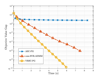
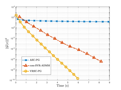
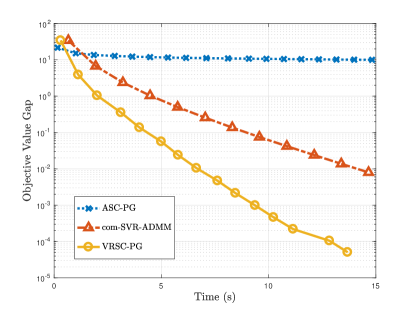
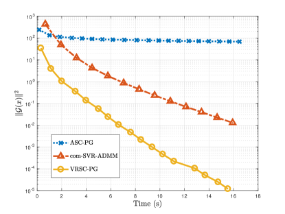
Figure 1 shows the convergence of compared methods regarding time. We suppose that the elapsed time is proportional to the query complexity. Objective value gap means $H(x_{t})-H(x^{*})$, where $x^{*}$ is the optimal solution to $H(x)$. We compute $H(x^{*})$ by running our method until convergence. Firstly, by observing the $x$ and $y$ axises in Figure 1, we can know that when $\kappa_{cov}=10$, all compared methods need more time to minimize problem (38), which is consistent with our analysis. Increasing $\kappa$ will increase the total query complexity. Secondly, we can also find out that com-SVR-ADMM and VRSC-PG admit linear convergence rate. ASC-PG runs faster at the beginning, because of their low query complexity in each iteration. However, their convergence slows down when the learning rate gets small. In four figures, our SVRC-PG always has the best performance compared to other compared methods.

5.2 Application to Reinforcement Learning

We then apply stochastic composition optimization to reinforcement learning and evaluate three compared methods in the task of policy evaluation. In reinforcement learning, let $V^{\pi}(s)$ be the value of state $s$ under policy $\pi$. The value function $V^{\pi}(s)$ can be evaluated through Bellman equation as follows:

$$V^{\pi}(s_{1})=\mathbb{E}[r_{s_{1},s_{2}}+\gamma V^{\pi}(s_{2})|s_{1}]$$ (39)

for all $s_{1},s_{2}\in\{1,2,...,S\}$, where $S$ represents the number of total states. According to [14], the Bellman equation (39) can also be written as a composition problem. In our experiment, we also add sparsity regularization $h(x)=\lambda|x|$ in the objective function.

Following [3], we generate a Markov decision process (MDP). There are $400$ states and $10$ actions at each state. The transition probability is generated randomly from the uniform distribution in the range of $[0,1]$. We then add $10^{-5}$ to each element of transition matrix to ensure the ergodicity of our MDP. The rewards $r(s,s^{\prime})$ from state $s$ to state $s^{\prime}$ are also sampled uniformly in the range of $[0,1]$. In our experiment, we set $\lambda=10^{-3}$ and $A=B=b_{1}=5$. We also select these values casually, better results can be obtained if we tune them carefully.

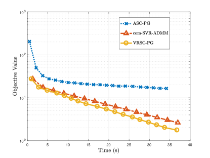
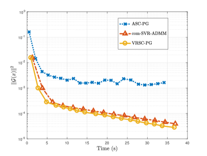
In Figure 2, we plot the convergence of the objective value and $\|\mathcal{G}(x)\|^{2}$ in terms of time. We can observe that VRSC-PG is much faster than ASC-PG, which has been reflected in the analysis of convergence rate already. It is also obvious that our VRSC-PG converges faster than com-SVR-ADMM. Experimental results on policy evaluation also verify our theoretical analysis.

6 Conclusion

In this paper, we propose variance reduced stochastic compositional proximal gradient method (VRSC-PG) for composition problem with nonsmooth regularization penalty. We also analyze the convergence rate of our method: (1) for strongly convex composition problem, VRSC-PG is proved to admit linear convergence; (2) for general composition problem, VRSC-PG significantly improves the state-of-the-art convergence rate from $O(T^{-1/2})$ to $O((n_{1}+n_{2})^{{2}/{3}}T^{-1})$. Both of our theoretical analysis, to the best of our knowledge, are the state-of-the-art results for stochastic composition optimization. Finally, we apply our method to two different applications, portfolio management and reinforcement learning. Experimental results show that our method always has the best performance in different cases and verify the conclusions of theoretical analysis.

Appendix A Strongly Convex Problem

Proof to Lemma 1

Proof 1

Following [15], we define function $\phi_{i}(x)$:

$$\phi_{i}(x)=F_{i}(G(x))-F_{i}(G(x^{*}))-\left<(\nabla G(x^{*}))^{T}\nabla F_{i}(G(x^{*})),(x-x^{*})\right>$$ (40)

where $x^{*}=\arg\min_{x}H(x)$ denotes the optimal solution of $H(x)$. It is easy to know that $\nabla\phi_{i}(x^{*})=0$ and $\min_{x}\phi_{i}(x)=\phi_{i}(x^{*})=0$. For any $x,y\in\mathbb{R}^{N}$, we have:

$$\|\nabla\phi_{i}(x)-\nabla\phi_{i}(y)\|$$ (41)

$$= \|(\nabla G(x))^{T}\nabla F_{i}(G(x))-(\nabla G(y))^{T}\nabla F_{i}(G(y))\|$$

$$= \|\frac{1}{n_{2}}\sum\limits_{j=1}^{n_{2}}(\nabla G_{j}(x))^{T}F_{i}(G(x))-\frac{1}{n_{2}}\sum\limits_{j=1}^{n_{2}}(\nabla G_{j}(y))^{T}F_{i}(G(y))\|$$

$$\leq \frac{1}{n_{2}}\sum\limits_{j=1}^{n_{2}}\|(\nabla G_{j}(x))^{T}F_{i}(G(x))-(\nabla G_{j}(y))^{T}F_{i}(G(y))\|$$

$$\leq L_{f}\|x-y\|$$

where the first inequality follows from the triangle inequality, and the second inequality follows from (19) in Assumption 3. Therefore, $\nabla\phi_{i}(x)$ is $L_{f}$-Lipschitz continuous. According to Theorem 2.1.5 in [10], we have:

$$\frac{1}{2L_{f}}\|\nabla\phi_{i}(x)-\nabla\phi_{i}(x^{*})\|^{2} \leq \phi_{i}(x)-\phi_{i}(x^{*})-\left<\nabla\phi_{i}(x^{*}),x-x^{*}\right>$$ (42)

Because $\phi_{i}(x^{*})=0$ and $\nabla\phi_{i}(x^{*})=0$, it follows that:

$$\frac{1}{2L_{f}}\|(\nabla G(x))^{T}\nabla F_{i}(G(x))-(\nabla G(x^{*}))^{T}\nabla F_{i}(G(x^{*}))\|^{2}$$ (43)

$$\leq F_{i}(G(x))-F_{i}(G(x^{*}))-\left<(\nabla G(x^{*}))^{T}\nabla F_{i}(G(x^{*})),(x-x^{*})\right>$$

Because $x^{*}=\arg\min_{x}f(x)+h(x)$, there exists $\xi^{*}\in\partial h(x^{*})$ so that $(\nabla G(x^{*}))^{T}\nabla F(G(x^{*}))+\xi^{*}=0$. Then it holds that:

$$\frac{1}{n_{1}}\sum\limits_{i=1}^{n_{1}}\|(\nabla G(x))^{T}\nabla F_{i}(G(x))-(\nabla G(x^{*}))^{T}\nabla F_{i}(G(x^{*}))\|^{2}$$ (44)

$$\leq 2L_{f}\bigg{[}F(G(x))-F(G(x^{*}))-\left<(\nabla G(x^{*}))^{T}\nabla F(G(x^{*})),(x-x^{*})\right>\bigg{]}$$

$$= 2L_{f}\bigg{[}F(G(x))-F(G(x^{*}))+\left<\xi^{*},(x-x^{*})\right>\bigg{]}$$

$$\leq 2L_{f}\bigg{[}F(G(x))-F(G(x^{*}))+h(x)-h(x^{*})\bigg{]}$$

$$\leq 2L_{f}\bigg{[}H(x)-H(x^{*})\bigg{]}$$

where the third inequality is from the convexity of $h(x)$. We let $u_{t}$ be the unbiased estimate of $\nabla f(x_{t}^{s+1})$:

$${u}_{t}^{s+1}=\frac{1}{b_{1}}\sum\limits_{i_{t}\in I_{t}}\biggl{(}\left(\nabla G({x}_{t}^{s+1})\right)^{T}\nabla F_{i_{t}}({G}(x_{t}^{s+1}))-\left(\nabla G(\tilde{x}^{s})\right)^{T}\nabla F_{i_{t}}(\tilde{G}^{s})\biggr{)}+\nabla f(\tilde{x}^{s})$$ (45)

where $\mathbb{E}{u}_{t}^{s+1}=\nabla f({x}_{t}^{s+1})$. We can get the upper bound of the variance of $u_{t}$:

$$\mathbb{E}\|u_{t}-\nabla f(x_{t}^{s+1})\|^{2}$$ (46)

$$= \mathbb{E}\|\frac{1}{b_{1}}\sum\limits_{i_{t}\in I_{t}}\biggl{(}\left(\nabla G({x}_{t}^{s+1})\right)^{T}\nabla F_{i_{t}}({G}(x_{t}^{s+1}))-\left(\nabla G(\tilde{x}^{s})\right)^{T}\nabla F_{i_{t}}(\tilde{G}^{s})+\nabla f(\tilde{x}^{s})-\nabla f(x_{t}^{s+1})\biggr{)}\|^{2}$$

$$= \frac{1}{b_{1}}\sum\limits_{i_{t}\in I_{t}}\mathbb{E}\|\left(\nabla G({x}_{t}^{s+1})\right)^{T}\nabla F_{i_{t}}({G}(x_{t}^{s+1}))-\left(\nabla G(\tilde{x}^{s})\right)^{T}\nabla F_{i_{t}}(\tilde{G}^{s})+\nabla f(\tilde{x}^{s})-\nabla f(x_{t}^{s+1})\|^{2}$$

$$\leq \frac{1}{b_{1}}\sum\limits_{i_{t}\in I_{t}}\mathbb{E}\|\left(\nabla G({x}_{t}^{s+1})\right)^{T}\nabla F_{i_{t}}({G}(x_{t}^{s+1}))-\left(\nabla G(\tilde{x}^{s})\right)^{T}\nabla F_{i_{t}}(\tilde{G}^{s})\|^{2}$$

$$\leq \frac{2}{b_{1}}\sum\limits_{i_{t}\in I_{t}}\biggl{(}\mathbb{E}\|\left(\nabla G({x}_{t}^{s+1})\right)^{T}\nabla F_{i_{t}}(G(x_{t}^{s+1}))-\left(\nabla G({x^{*}})\right)^{T}\nabla F_{i_{t}}(G(x^{*}))\|^{2}$$

$$+\mathbb{E}\|\left(\nabla G({\tilde{x}^{s}})\right)^{T}\nabla F_{i_{t}}(G(\tilde{x}^{s}))-\left(\nabla G({x^{*}})\right)^{T}\nabla F_{i_{t}}(G(x^{*}))\|^{2}\biggr{)}$$

$$\leq 4L_{f}\bigg{[}H(x_{t}^{s+1})-H(x^{*})+H(\tilde{x}^{s})-H(x^{*})\bigg{]}$$

where the second equality follows from Lemma 4, the last inequality follows from (44) Then, we compute the upper bound of $\mathbb{E}\left\|{u}_{t}^{s+1}-{v}_{t}^{s+1}\right\|^{2}$:

$$\mathbb{E}\left\|{u}_{t}^{s+1}-{v}_{t}^{s+1}\right\|^{2} = \mathbb{E}\left\|\frac{1}{b_{1}}\sum\limits_{i_{t}\in I_{t}}\biggl{(}\left(\nabla G({x}_{t}^{s+1})\right)^{T}\nabla F_{i_{t}}({G}(x_{t}^{s+1}))-\left(\nabla\widehat{G}_{t}^{s+1}\right)^{T}\nabla F_{i_{t}}(\widehat{G}_{t}^{s+1})\biggr{)}\right\|^{2}$$

$$\leq \frac{1}{b_{1}}\sum\limits_{i_{t}\in I_{t}}\underbrace{\mathbb{E}\left\|\left(\nabla G({x}_{t}^{s+1})\right)^{T}\nabla F_{i_{t}}({G}(x_{t}^{s+1}))-\left(\nabla\widehat{G}_{t}^{s+1}\right)^{T}\nabla F_{i_{t}}(\widehat{G}_{t}^{s+1})\right\|^{2}}_{T_{1}}$$

where the inequality follows from Lemma 4. Then we can get the upper bound of $T_{3}$ as follows:

$$T_{1} \leq 2\mathbb{E}\left\|\left(\nabla G({x}_{t}^{s+1})\right)^{T}\nabla F_{i_{t}}({G}(x_{t}^{s+1}))-\left(\nabla G(x_{t}^{s+1})\right)^{T}\nabla F_{i_{t}}(\widehat{G}_{t}^{s+1})\right\|^{2}$$ (48)

$$+2\mathbb{E}\left\|\left(\nabla G(x_{t}^{s+1})\right)^{T}\nabla F_{i_{t}}(\widehat{G}_{t}^{s+1})-\left(\nabla\widehat{G}_{t}^{s+1}\right)^{T}\nabla F_{i_{t}}(\widehat{G}_{t}^{s+1})\right\|^{2}$$

$$\leq 2B_{F}^{2}\mathbb{E}\left\|\left(\nabla G(x_{t}^{s+1})\right)^{T}-\left(\nabla\widehat{G}_{t}^{s+1}\right)^{T}\right\|^{2}+2B_{G}^{2}\mathbb{E}\left\|\nabla F_{i_{t}}({G}(x_{t}^{s+1}))-\nabla F_{i_{t}}(\widehat{G}_{t}^{s+1})\right\|^{2}$$

$$\leq 2B_{F}^{2}\mathbb{E}\left\|\left(\nabla G(x_{t}^{s+1})\right)^{T}-\left(\nabla G(\tilde{x}^{s})-\frac{1}{B}\sum\limits_{1\leq j\leq B}(\nabla G_{B_{t}[j]}(\tilde{x}^{s})-\nabla G_{B_{t}[j]}(x_{t}^{s+1}))\right)^{T}\right\|^{2}$$

$$+2B_{G}^{2}L_{F}^{2}\mathbb{E}\left\|{G}(x_{t}^{s+1})-\left(G^{s}-\frac{1}{A}\sum\limits_{1\leq j\leq A}(G_{A_{t}[j]}(\tilde{x}^{s})-G_{A_{t}[j]}(x_{t}^{s+1}))\right)\right\|^{2}$$

$$= \frac{2B_{F}^{2}}{B^{2}}\mathbb{E}\left\|\sum\limits_{1\leq j\leq B}\left(\nabla G_{B_{t}[j]}(\tilde{x}^{s})-\nabla G_{B_{t}[j]}(x_{t}^{s+1})+\nabla G(x_{t}^{s+1})-\nabla G(\tilde{x}^{s})\right)^{T}\right\|^{2}$$

$$+\frac{2B_{G}^{2}L_{F}^{2}}{A^{2}}\mathbb{E}\left\|\sum\limits_{1\leq j\leq A}\left(G_{A_{t}[j]}(\tilde{x}^{s})-G_{A_{t}[j]}(x_{t}^{s+1})+{G}(x_{t}^{s+1})-G^{s}\right)\right\|^{2}$$

$$= \frac{2B_{F}^{2}}{B^{2}}\sum\limits_{1\leq j\leq B}\mathbb{E}\left\|\left(\nabla G_{B_{t}[j]}(\tilde{x}^{s})-\nabla G_{B_{t}[j]}(x_{t}^{s+1})+\nabla G(x_{t}^{s+1})-\nabla G(\tilde{x}^{s})\right)^{T}\right\|^{2}$$

$$+\frac{2B_{G}^{2}L_{F}^{2}}{A^{2}}\sum\limits_{1\leq j\leq A}\mathbb{E}\left\|\left(G_{A_{t}[j]}(\tilde{x}^{s})-G_{A_{t}[j]}(x_{t}^{s+1})+{G}(x_{t}^{s+1})-G^{s}\right)\right\|^{2}$$

$$\leq \frac{2B_{F}^{2}}{B^{2}}\sum\limits_{1\leq j\leq B}8L_{G}^{2}\left(\mathbb{E}\|\tilde{x}^{s}-x^{*}\|^{2}+\mathbb{E}\|x_{t}^{s+1}-x^{*}\|^{2}\right)$$

$$+\frac{2B_{G}^{2}L_{F}^{2}}{A^{2}}\sum\limits_{1\leq j\leq A}8B_{G}\left(\mathbb{E}\|\tilde{x}^{s}-x^{*}\|^{2}+\mathbb{E}\|x_{t}^{s+1}-x^{*}\|^{2}\right)$$

$$= 16\left(\frac{B_{F}^{2}L_{G}^{2}}{B}+\frac{B_{G}^{4}L_{F}^{2}}{A}\right)\mathbb{E}\left(\|x^{s+1}_{t}-x^{*}\|^{2}+\|\tilde{x}^{s}-x^{*}\|^{2}\right)$$

$$\leq \frac{32}{\mu}\left(\frac{B_{F}^{2}L_{G}^{2}}{B}+\frac{B_{G}^{4}L_{F}^{2}}{A}\right)\mathbb{E}\left(H({x}_{t}^{s+1})-H({x}^{*})+H(\tilde{x}^{s})-H({x}^{*})\right)$$

where the first inequality follows from Lemma 4, the second, third fourth inequality follows from Assumption 3, the third equality follows from Lemma 3, the last inequality follows from the strong convexity of $H(x)$, such that $\|x-x^{*}\|^{2}\leq\frac{2}{\mu}(H(x)-H(x^{*}))$. Combine (46) and (1), then we have:

$$\mathbb{E}\|v_{t}-\nabla f(x_{t}^{s+1})\|^{2}$$ (49)

$$\leq 2\mathbb{E}\left\|{u}_{t}^{s+1}-{v}_{t}^{s+1}\right\|^{2}+2\mathbb{E}\|u_{t}-\nabla f(x_{t}^{s+1})\|$$

$$\leq \biggl{(}\frac{64}{\mu}\left(\frac{B_{F}^{2}L_{G}^{2}}{B}+\frac{B_{G}^{4}L_{F}^{2}}{A}\right)+{8L_{f}}\biggr{)}\biggl{[}H(x_{t}^{s+1})-H(x^{*})+H(\tilde{x}^{s})-H(x^{*})\biggr{]}$$

where the first inequality follows from Lemma 4.

Lemma 2

Suppose all assumption hold, given $x^{*}$ is the optimal solution to problem $H(x)$, there exists a constant $\alpha>0$ such that:

$$\mathbb{E}\left\langle{v}_{t}^{s+1}-\nabla f({x}_{t}^{s+1}),x^{*}-x^{s+1}_{t+1}\right\rangle$$ (50)

$$\leq \left(6\eta L_{f}+\left(\frac{\eta}{2}+\frac{1}{2\alpha}\right)\frac{32}{\mu}\left(\frac{B_{F}^{2}L_{G}^{2}}{B}+\frac{B_{G}^{4}L_{F}^{2}}{A}\right)\right)\mathbb{E}\left(H({x}_{t}^{s+1})-H({x}^{*})+H(\tilde{x}^{s})-H({x}^{*})\right)$$

$$+\frac{\alpha}{\mu}\mathbb{E}\left(H({x}_{t+1}^{s+1})-H({x}^{*})\right)$$

Proof 2

Define $\bar{x}^{s+1}_{t+1}=\textrm{Prox}_{\eta h(\cdot)}\left(x^{s+1}_{t}-{\eta}\nabla f({x}_{t}^{s+1})\right)$, we have that

$$\mathbb{E}\left\langle{v}_{t}^{s+1}-\nabla f({x}_{t}^{s+1}),x^{*}-x^{s+1}_{t+1}\right\rangle$$ (51)

$$= \mathbb{E}\left\langle{u}_{t}^{s+1}-\nabla f({x}_{t}^{s+1}),x^{*}-x^{s}_{t+1}\right\rangle+\mathbb{E}\left\langle{v}_{t}^{s+1}-{u}_{t}^{s+1},x^{*}-x^{s+1}_{t+1}\right\rangle$$

$$= \underbrace{\mathbb{E}\left\langle{u}_{t}^{s+1}-\nabla f({x}_{t}^{s+1}),x^{*}-\bar{x}^{s+1}_{t+1}\right\rangle}_{=0}+\mathbb{E}\left\langle{u}_{t}^{s+1}-\nabla f({x}_{t}^{s+1}),\bar{x}_{t+1}^{s+1}-x^{s+1}_{t+1}\right\rangle$$

$$+\mathbb{E}\left\langle{v}_{t}^{s+1}-{u}_{t}^{s+1},x^{*}-x^{s+1}_{t+1}\right\rangle$$

$$\leq \mathbb{E}\left\|{u}_{t}^{s+1}-\nabla f({x}_{t}^{s+1})\right\|\left\|\bar{x}_{t+1}^{s+1}-x^{s+1}_{t+1}\right\|+\mathbb{E}\left\langle{v}_{t}^{s+1}-{u}_{t}^{s+1},x^{*}-x^{s+1}_{t+1}\right\rangle$$

$$\leq \eta\mathbb{E}\left\|{u}_{t}^{s+1}-\nabla f({x}_{t}^{s+1})\right\|\left\|\nabla f({x}_{t}^{s+1})-{v}_{t}^{s+1}\right\|+\mathbb{E}\left\langle{v}_{t}^{s+1}-{u}_{t}^{s+1},x^{*}-x^{s+1}_{t+1}\right\rangle$$

$$\leq \eta\mathbb{E}\left\|{u}_{t}^{s+1}-\nabla f({x}_{t}^{s+1})\right\|\left(\left\|\nabla f({x}_{t}^{s+1})-{u}_{t}^{s+1}\right\|+\left\|{u}_{t}^{s+1}-{v}_{t}^{s+1}\right\|\right)$$

$$+\frac{1}{2\alpha}\mathbb{E}\left\|{v}_{t}^{s+1}-{u}_{t}^{s+1}\right\|^{2}+\frac{\alpha}{2}\mathbb{E}\left\|x^{*}-x^{s+1}_{t+1}\right\|^{2}$$

$$\leq \eta\mathbb{E}\left\|{u}_{t}^{s+1}-\nabla f({x}_{t}^{s+1})\right\|^{2}+\frac{\eta}{2}\mathbb{E}\left\|{u}_{t}^{s+1}-\nabla f({x}_{t}^{s+1})\right\|^{2}+\frac{\eta}{2}\left\|{u}_{t}^{s+1}-{v}_{t}^{s+1}\right\|^{2}$$

$$+\frac{1}{2\alpha}\mathbb{E}\left\|{v}_{t}^{s+1}-{u}_{t}^{s+1}\right\|^{2}+\frac{\alpha}{2}\mathbb{E}\left\|x^{*}-x^{s+1}_{t+1}\right\|^{2}$$

$$= \frac{3}{2}\eta{\mathbb{E}\left\|{u}_{t}^{s+1}-\nabla f({x}_{t}^{s+1})\right\|^{2}}+\left(\frac{\eta}{2}+\frac{1}{2\alpha}\right){\mathbb{E}\left\|{u}_{t}^{s+1}-{v}_{t}^{s+1}\right\|^{2}}+\frac{\alpha}{2}\mathbb{E}\left\|x^{*}-x^{s+1}_{t+1}\right\|^{2}$$

$$\leq \left(6\eta L_{f}+\left(\frac{\eta}{2}+\frac{1}{2\alpha}\right)\frac{32}{\mu}\left(\frac{B_{F}^{2}L_{G}^{2}}{B}+\frac{B_{G}^{4}L_{F}^{2}}{A}\right)\right)\mathbb{E}\left(H({x}_{t}^{s+1})-H({x}^{*})+H(\tilde{x}^{s})-H({x}^{*})\right)$$

$$+\frac{\alpha}{\mu}\mathbb{E}\left(H({x}_{t+1}^{s+1})-H({x}^{*})\right)$$

where the third inequality follows from triangle inequality and Young’s inequality, the last inequality follows from Lemma 1. This completes the proof.

Proof to Theorem 1

Proof 3

We define the virtual gradient $g_{t}^{s+1}$ as follows:

$$g_{t}^{s+1}=\frac{1}{\eta}\left(x^{s+1}_{t}-\textrm{Prox}_{\eta h(\cdot)}\left(x^{s+1}_{t}-{\eta}{v}^{s+1}_{t}\right)\right)$$ (52)

Because $x^{s+1}_{t+1}={\arg\min}_{x}\frac{1}{2\eta}\|x-(x_{t}^{s+1}-{\eta}{v}^{s+1}_{t})\|^{2}+h(x)$, based on the optimality condition, we have that $\frac{1}{\eta}\left(-x_{t+1}^{s+1}+(x_{t}^{s+1}-{\eta}{v}_{t}^{s+1})\right)\in\partial h(x_{t+1}^{s+1})$. Thus, we have:

$$g_{t}^{s+1}=\frac{1}{\eta}\left(x_{t}^{s+1}-x_{t+1}^{s+1}\right)={v}^{s+1}_{t}+\xi_{t}^{s+1}$$ (53)

where $\xi_{t}^{s+1}\in\partial h(x_{t+1}^{s+1})$. Note that the virtual gradients $g_{t}^{s+1}$ are only used for the analysis, not computed in the implementation. Because $x^{*}$ is the optimal solution, we have:

$$H(x^{*}) = f(x^{*})+h(x^{*})$$ (54)

$$\geq f(x^{s+1}_{t})+\langle\nabla f(x_{t}^{s+1}),x^{*}-x_{t}^{s+1}\rangle+h(x_{t+1}^{s+1})+\langle\xi_{t}^{s+1},x^{*}-x_{t+1}^{s+1}\rangle$$

$$\geq f({x}_{t+1}^{s+1})-\langle\nabla f(x_{t}^{s+1}),x_{t+1}^{s+1}-x_{t}^{s+1}\rangle-\frac{L_{f}}{2}\|x^{s+1}_{t+1}-x^{s+1}_{t}\|^{2}$$

$$+\langle\nabla f(x_{t}^{s+1}),x^{*}-x_{t}^{s+1}\rangle+h(x_{t+1}^{s+1})+\langle\xi_{t}^{s+1},x^{*}-x_{t+1}^{s+1}\rangle$$

$$= H({x}_{t+1}^{s+1})+\langle v_{t}^{s+1}+\xi_{t}^{s+1},x^{*}-{x}_{t}^{s+1}\rangle+\langle v_{t}^{s+1}+\xi_{t}^{s+1},{x}_{t}^{s+1}-{x}_{t+1}^{s+1}\rangle$$

$$+\langle\nabla f(x_{t}^{s+1})-v_{t}^{s+1},x^{*}-x_{t+1}^{s+1}\rangle-\frac{L_{f}}{2}\|x_{t+1}^{s+1}-x_{t}^{s+1}\|^{2}$$

$$= H({x}_{t+1}^{s+1})+\langle g_{t}^{s+1},x^{*}-{x}_{t}^{s+1}\rangle+\eta\|g_{t}^{s+1}\|^{2}+\langle\nabla f(x_{t}^{s+1})-v_{t}^{s+1},x^{*}-x_{t+1}^{s+1}\rangle-\frac{L_{f}\eta^{2}}{2}\left\|g_{t}^{s+1}\right\|^{2}$$

where the first inequality uses the convexity of $F(x)$ and $R(x)$, the second inequality follows from that $f(x)$ is $L_{f}$-smooth. Thus, we have:

$$\langle g_{t}^{s+1},x^{*}-{x}_{t}^{s+1}\rangle$$ (55)

$$\leq H(x^{*})-H({x}_{t+1}^{s+1})-\eta\|g_{t}^{s+1}\|^{2}-\langle\nabla f(x_{t}^{s+1})-v_{t}^{s+1},x^{*}-x_{t+1}^{s+1}\rangle+\frac{L_{f}\eta^{2}}{2}\left\|g_{t}^{s+1}\right\|^{2}$$

As per the iteration of $x_{t}^{s+1}$, we have:

$$\mathbb{E}\left\|x^{s+1}_{t+1}-x^{*}\right\|^{2}=\mathbb{E}\left\|x^{s+1}_{t}-\eta g_{t}^{s+1}-x^{*}\right\|^{2}$$

$$= \mathbb{E}\left\|x_{t}^{s+1}-x^{*}\right\|^{2}+\eta^{2}\mathbb{E}\left\|g_{t}^{s+1}\right\|^{2}-2\eta\mathbb{E}\left\langle g_{t}^{s+1},x_{t}^{s+1}-x^{*}\right\rangle$$

$$\leq \mathbb{E}\left\|x_{t}^{s+1}-x^{*}\right\|^{2}+\eta^{2}\mathbb{E}\left\|g_{t}^{s+1}\right\|^{2}-2\eta(\mathbb{E}H(x_{t+1}^{s+1})-H(x^{*}))+$$

$$2\eta\mathbb{E}\langle\nabla f({x}_{t}^{s+1})-v_{t}^{s+1},x_{t+1}^{s+1}-x^{*}\rangle-2\eta^{2}\mathbb{E}\left\|g_{t}^{s+1}\right\|^{2}+{L_{f}\eta^{3}}\left\|g_{t}^{s+1}\right\|^{2}$$

$${\leq} \mathbb{E}\left\|x_{t}^{s+1}-x^{*}\right\|^{2}-2\eta(\mathbb{E}H(x_{t+1}^{s+1})-H(x^{*}))+2\eta\mathbb{E}\langle\nabla f({x}_{t}^{s+1})-v_{t}^{s+1},x_{t+1}^{s+1}-x^{*}\rangle$$

$$\leq \mathbb{E}\left\|x_{t}^{s+1}-x^{*}\right\|^{2}-2\eta(\mathbb{E}H(x_{t+1}^{s+1})-H(x^{*}))+2\eta\frac{\alpha}{\mu}\mathbb{E}\left(H({x}_{t+1}^{s+1})-H({x}^{*})\right)$$

$$+2\eta\left(6\eta L_{f}+\left(\frac{\eta}{2}+\frac{1}{2\alpha}\right)\frac{32}{\mu}\left(\frac{B_{F}^{2}L_{G}^{2}}{B}+\frac{B_{G}^{4}L_{F}^{2}}{A}\right)\right)\mathbb{E}\left(H({x}_{t}^{s+1})-H({x}^{*})+H(\tilde{x}^{s})-H({x}^{*})\right)$$

$$= \mathbb{E}\left\|x_{t}^{s+1}-x^{*}\right\|^{2}-2\eta\left(1-\frac{\alpha}{\mu}\right)(\mathbb{E}H(x_{t+1}^{s+1})-H(x^{*}))$$

$$+2\eta\left(6\eta L_{f}+\left(\frac{\eta}{2}+\frac{1}{2\alpha}\right)\frac{32}{\mu}\left(\frac{B_{F}^{2}L_{G}^{2}}{B}+\frac{B_{G}^{4}L_{F}^{2}}{A}\right)\right)\mathbb{E}\left(H({x}_{t}^{s+1})-H({x}^{*})+H(\tilde{x}^{s})-H({x}^{*})\right)$$

where the first inequality follows from (55), the second inequality follows from $\eta L_{f}\leq 1$, the third inequality follows from Lemma 2. By summing the inequality (3) over $t=0,\cdots,m-1$, because $\tilde{x}^{s+1}=x_{m}^{s+1}$ and $\tilde{x}^{s}=x_{0}^{s+1}$, we obtain the following inequality:

$$\mathbb{E}\left\|x^{s+1}_{m}-x^{*}\right\|^{2}+2\eta\left(1-\frac{\alpha}{\mu}\right)(\mathbb{E}H(x_{m}^{s+1})-H(x^{*}))+2\eta\left(1-\frac{\alpha}{\mu}\right)\sum_{t=1}^{m-1}(\mathbb{E}H(x_{t}^{s+1})-H(x^{*}))$$ (57)

$$\leq \mathbb{E}\left\|\tilde{x}^{s}-x^{*}\right\|^{2}+2\eta\left(6\eta L_{f}+\left(\frac{\eta}{2}+\frac{1}{2\alpha}\right)\frac{32}{\mu}\left(\frac{B_{F}^{2}L_{G}^{2}}{B}+\frac{B_{G}^{4}L_{F}^{2}}{A}\right)\right)\sum_{t=1}^{m-1}\mathbb{E}\left(H({x}_{t}^{s+1})-H({x}^{*})\right)$$

$$+2\eta\left(6\eta L_{f}+\left(\frac{\eta}{2}+\frac{1}{2\alpha}\right)\frac{32}{\mu}\left(\frac{B_{F}^{2}L_{G}^{2}}{B}+\frac{B_{G}^{4}L_{F}^{2}}{A}\right)\right)(m+1)\mathbb{E}\left(H(\tilde{x}^{s})-H({x}^{*})\right)$$

According to (57) and $\left\|\tilde{x}^{s}-x^{*}\right\|^{2}\leq\frac{2}{\mu}(H(\tilde{x})-H(x^{*}))$ , the following inequality holds:

$$2\eta\left(1-\frac{\alpha}{\mu}-\left(6\eta L_{f}+\left(\frac{\eta}{2}+\frac{1}{2\alpha}\right)\frac{32}{\mu}\left(\frac{B_{F}^{2}L_{G}^{2}}{B}+\frac{B_{G}^{4}L_{F}^{2}}{A}\right)\right)\right)\sum_{t=1}^{m}(\mathbb{E}H(x_{t}^{s+1})-H(x^{*}))$$ (58)

$$\leq \left(\frac{2}{\mu}+2\eta\left(6\eta L_{f}+\left(\frac{\eta}{2}+\frac{1}{2\alpha}\right)\frac{32}{\mu}\left(\frac{B_{F}^{2}L_{G}^{2}}{B}+\frac{B_{G}^{4}L_{F}^{2}}{A}\right)\right)(m+1)\right)\mathbb{E}\left(H(\tilde{x}^{s})-H({x}^{*})\right)$$

As per the convexity of $H(x)$ and the definition of $\tilde{x}^{s+1}$, we have $H(\tilde{x}^{s+1})\leq\frac{1}{m}\sum\limits_{t=1}^{m}H(x_{t}^{s+1})$. According to (58), and let $\alpha=\frac{\mu}{8}$, we have that:

$$\mathbb{E}H(\tilde{x}^{s+1})-H(x^{*})$$ (59)

$$\leq \frac{\frac{2}{\mu}+2\eta\left(6\eta L_{f}+\left(\frac{\eta}{2}+\frac{4}{\mu}\right)\frac{32}{\mu}\left(\frac{B_{F}^{2}L_{G}^{2}}{B}+\frac{B_{G}^{4}L_{F}^{2}}{A}\right)\right)(m+1)}{2\eta\left(\frac{7}{8}-\left(6\eta L_{f}+\left(\frac{\eta}{2}+\frac{4}{\mu}\right)\frac{32}{\mu}\left(\frac{B_{F}^{2}L_{G}^{2}}{B}+\frac{B_{G}^{4}L_{F}^{2}}{A}\right)\right)\right)m}\mathbb{E}H(\tilde{x}^{s})-H({x}^{*})$$

Define $\rho=\frac{\frac{2}{\mu}+2\eta\left(6\eta L_{f}+\left(\frac{\eta}{2}+\frac{4}{\mu}\right)\frac{32}{\mu}\left(\frac{B_{F}^{2}L_{G}^{2}}{B}+\frac{B_{G}^{4}L_{F}^{2}}{A}\right)\right)(m+1)}{2\eta\left(\frac{7}{8}-\left(6\eta L_{f}+\left(\frac{\eta}{2}+\frac{4}{\mu}\right)\frac{32}{\mu}\left(\frac{B_{F}^{2}L_{G}^{2}}{B}+\frac{B_{G}^{4}L_{F}^{2}}{A}\right)\right)\right)m}$, where $\rho<1$. Applying (59) recursively, we have:

$$\mathbb{E}H(\tilde{x}^{S})-H(x^{*})\leq\rho^{S}\bigg{(}H(x^{0})-H(x^{*})\biggr{)}$$ (60)

This completes the proof.

Proof to Corollary 1

Proof 4

Appropriately choosing $\eta$, $m$ and $A$ in Algorithm 3, we can get the linear convergence rate for our algorithm. We choose $A$ and $B$ to satisfy:

$$\frac{\eta}{2}\frac{32B_{F}^{2}L_{G}^{2}}{B\mu} \leq \frac{1}{16}$$ (61)

$$\frac{\eta}{2}\frac{32B_{G}^{4}L_{F}^{2}}{A\mu} \leq \frac{1}{16}$$ (62)

$$\frac{4}{\mu}\frac{32B_{F}^{2}L_{G}^{2}}{B\mu} \leq \frac{1}{16}$$ (63)

$$\frac{4}{\mu}\frac{32B_{G}^{4}L_{F}^{2}}{A\mu} \leq \frac{1}{16}$$ (64)

The above inequalities are equivalent with the following conditions:

$$A \geq \max\left\{\frac{256\eta B_{G}^{4}L_{F}^{2}}{\mu},\frac{2048B_{G}^{4}L_{F}^{2}}{\mu^{2}}\right\}$$ (65)

$$B \geq \max\left\{\frac{256\eta B_{F}^{2}L_{G}^{2}}{\mu},\frac{2048B_{F}^{2}L_{G}^{2}}{\mu^{2}}\right\}$$ (66)

We choose $\eta$ satisfying $6\eta L_{f}\leq\frac{1}{16}$, such that $\eta\leq\frac{1}{96L_{f}}$. It follows that:

$$\frac{\frac{2}{\mu}+2\eta\left(6\eta L_{f}+\left(\frac{\eta}{2}+\frac{4}{\mu}\right)\frac{32}{\mu}\left(\frac{B_{F}^{2}L_{G}^{2}}{B}+\frac{B_{G}^{4}L_{F}^{2}}{A}\right)\right)(m+1)}{2\eta\left(\frac{7}{8}-\left(6\eta L_{f}+\left(\frac{\eta}{2}+\frac{4}{\mu}\right)\frac{32}{\mu}\left(\frac{B_{F}^{2}L_{G}^{2}}{B}+\frac{B_{G}^{4}L_{F}^{2}}{A}\right)\right)\right)m}$$ (67)

$$\leq \frac{\frac{2}{\mu m}+2\eta\frac{5}{16}(1+\frac{1}{m})}{2\eta\frac{9}{16}}$$

$$= \frac{5}{9}+\frac{\frac{2}{\mu m}+2\eta\frac{1}{m}}{2\eta\frac{9}{16}}$$

We then set $m$ satisfying $\frac{\frac{2}{\mu m}+2\eta\frac{1}{m}}{2\eta\frac{9}{16}}\leq\frac{1}{9}$, which is equivalent to $m\geq 16\left(1+\frac{1}{\mu\eta}\right)$. Thus, by setting $\eta$, $m$, $A$ and $B$ appropriately:

$$\eta = \frac{1}{96L_{f}}$$ (68)

$$m = 16\left(1+\frac{96L_{f}}{\mu}\right)$$ (69)

$$A = \max\left\{\frac{8B_{G}^{4}L_{F}^{2}}{3\mu L_{f}},\frac{2048B_{G}^{4}L_{F}^{2}}{\mu^{2}}\right\}$$ (70)

$$B = \max\left\{\frac{8B_{F}^{2}L_{G}^{2}}{3\mu L_{f}},\frac{2048B_{F}^{2}L_{G}^{2}}{\mu^{2}}\right\}$$ (71)

we can obtain a linear convergence rate $\frac{2}{3}$. This completes the proof.

Appendix B General Problem

Proof to Theorem 2

Proof 5

We define $u_{t}^{s+1}$ to be an unbiased estimate for $\nabla f(x_{t}^{s+1})$:

$${u}_{t}^{s+1} = \frac{1}{b_{1}}\sum\limits_{i_{t}\in I_{t}}\biggl{(}\left(\nabla G({x}_{t}^{s+1})\right)^{T}\nabla F_{i_{t}}({G}(x_{t}^{s+1}))-\left(\nabla G(\tilde{x}^{s})\right)^{T}\nabla F_{i_{t}}({G}^{s})\biggr{)}+\nabla f(\tilde{x}^{s})$$ (72)

where $I_{t}$ is uniformly sampled from $\{1,2,...,n_{1}\}$ such that $|I_{t}|=b_{1}$. We also define:

$$\bar{x}_{t+1}^{s+1} = \text{Prox}_{\eta h(.)}(x_{t+1}^{s+1}-\eta\nabla f(x_{t}^{s+1}))$$ (73)

According to Lemma 2 in [12], if $y=prox_{\eta h}(x-\eta d^{\prime}),d^{\prime}\in\mathbb{R}^{d}$ and $\forall z\in\mathbb{R}^{d}$, following equality holds that:

$$H(y)\leq H(z)+\left<y-z,\nabla f(x)-d^{\prime}\right>+\bigg{[}\frac{L_{f}}{2}-\frac{1}{2\eta}\bigg{]}\|y-x\|^{2}+\bigg{[}\frac{L_{f}}{2}+\frac{1}{2\eta}\bigg{]}\|z-x\|^{2}-\frac{1}{2\eta}\|y-z\|^{2}$$ (74)

Thus if we let $y=\bar{x}_{t+1}^{s+1}$, $x=z=x_{t}^{s+1}$ and $d^{\prime}=\nabla f(x_{t}^{s+1})$, we have:

$$\mathbb{E}[H(\bar{x}_{t+1}^{s+1})] \leq \mathbb{E}\bigg{[}H(x_{t}^{s+1})+\bigg{[}\frac{L_{f}}{2}-\frac{1}{2\eta}\bigg{]}\|\bar{x}_{t+1}^{s+1}-x_{t}^{s+1}\|^{2}-\frac{1}{2\eta}\|\bar{x}_{t+1}^{s+1}-x_{t}^{s+1}\|^{2}\bigg{]}.$$ (75)

If we let $y=x_{t+1}^{s+1}$, $x=x_{t}^{s+1}$, $z=\bar{x}_{t+1}^{s+1}$ and $d^{\prime}=v_{t}^{s+1}$, then we have:

$$\mathbb{E}[H({x}_{t+1}^{s+1})] \leq \mathbb{E}\bigg{[}H(x_{t}^{s+1})+\bigg{[}\frac{L_{f}}{2}-\frac{1}{2\eta}\bigg{]}\|\bar{x}_{t+1}^{s+1}-x_{t}^{s+1}\|^{2}+\bigg{[}\frac{L_{f}}{2}+\frac{1}{2\eta}\bigg{]}\|x_{t+1}^{s+1}-x_{t}^{s+1}\|^{2}$$ (76)

$$-\frac{1}{2\eta}\|\bar{x}_{t+1}^{s+1}-x_{t}^{s+1}\|^{2}+\left<x_{t+1}^{s+1}-\bar{x}_{t+1}^{s+1},\nabla f(x_{t}^{s+1})-v_{t}^{s+1}\right>\bigg{]}.$$

Combine (75) and (76), we have:

$$\mathbb{E}[H(x_{t+1}^{s+1})] \leq \mathbb{E}\bigg{[}H(x_{t}^{s+1})+\bigg{[}L_{f}-\frac{1}{2\eta}\bigg{]}\|\bar{x}_{t+1}^{s+1}-x_{t}^{s+1}\|^{2}+\bigg{[}\frac{L_{f}}{2}-\frac{1}{2\eta}\bigg{]}\|x_{t+1}^{s+1}-x_{t}^{s+1}\|^{2}$$ (77)

$$-\frac{1}{2\eta}\|x_{t+1}^{s+1}-\bar{x}_{t+1}^{s+1}\|^{2}+\underbrace{\left<x_{t+1}^{s+1}-\bar{x}_{t+1}^{s+1},\nabla f(x_{t}^{s+1})-v_{t}^{s+1}\right>}_{T_{1}}\bigg{]}.$$

Then we can have an upper bound of $T_{1}$:

$$\mathbb{E}[T_{1}] \leq \frac{1}{2\eta}\mathbb{E}\|x_{t+1}^{s+1}-\tilde{x}_{t+1}^{s+1}\|^{2}+\frac{\eta}{2}\|\nabla f(x_{t}^{s+1})-v_{t}^{s+1}\|^{2}$$ (78)

$$\leq \frac{1}{2\eta}\mathbb{E}\|x_{t+1}^{s+1}-\tilde{x}_{t+1}^{s+1}\|^{2}+{\eta}\mathbb{E}\|\nabla f(x_{t}^{s+1})-u_{t}^{s+1}\|^{2}+{\eta}\mathbb{E}\|v_{t}^{s+1}-u_{t}^{s+1}\|^{2}$$

where the first inequality follows from Cauchy-Schwarz and Young’s inequality. As per the definition of $u_{t}^{s+1}$, we have:

$$\mathbb{E}\|\nabla f(x_{t}^{s+1})-u_{t}^{s+1}\|^{2}$$ (79)

$$= \mathbb{E}\|\frac{1}{b_{1}}\sum\limits_{i_{t}\in I_{t}}\biggl{(}\nabla f(x_{t}^{s+1})-\left(\nabla G({x}_{t}^{s+1})\right)^{T}\nabla F_{i_{t}}({G}(x_{t}^{s+1}))$$

$$+\left(\nabla G(\tilde{x}^{s})\right)^{T}\nabla F_{i_{t}}({G}^{s})-\nabla f(\tilde{x}^{s})\biggr{)}\|^{2}$$

$$= \frac{1}{b_{1}^{2}}\mathbb{E}\|\sum\limits_{i_{t}\in I_{t}}\biggl{(}\nabla f(x_{t}^{s+1})-\left(\nabla G({x}_{t}^{s+1})\right)^{T}\nabla F_{i_{t}}({G}(x_{t}^{s+1}))$$

$$+\left(\nabla G(\tilde{x}^{s})\right)^{T}\nabla F_{i_{t}}({G}^{s})-\nabla f(\tilde{x}^{s})\biggr{)}\|^{2}$$

$$= \frac{1}{b_{1}^{2}}\mathbb{E}\sum\limits_{i_{t}\in I_{t}}\|\nabla f(x_{t}^{s+1})-\left(\nabla G({x}_{t}^{s+1})\right)^{T}\nabla F_{i_{t}}({G}(x_{t}^{s+1}))$$

$$+\left(\nabla G(\tilde{x}^{s})\right)^{T}\nabla F_{i_{t}}({G}^{s})-\nabla f(\tilde{x}^{s})\|^{2}$$

$$\leq \frac{1}{b_{1}^{2}}\mathbb{E}\sum\limits_{i_{t}\in I_{t}}\|\left(\nabla G({x}_{t}^{s+1})\right)^{T}\nabla F_{i_{t}}({G}(x_{t}^{s+1}))-\left(\nabla G(\tilde{x}^{s})\right)^{T}\nabla F_{i_{t}}({G}^{s})\|^{2}$$

$$\leq \frac{L_{f}^{2}}{b_{1}}\mathbb{E}\|x_{t}^{s+1}-\tilde{x}^{s}\|^{2}$$

where the third equality follows from Lemma 3, the first inequality follows from:

$$\mathbb{E}\|\xi-\mathbb{E}[\xi]\|^{2} = \mathbb{E}\|\xi\|^{2}-\|\mathbb{E}[\xi]\|^{2},$$ (80)

and the last inequality follows from Assumption 2. We can bound $\mathbb{E}\|v_{t}^{s+1}-u_{t}^{s+1}\|^{2}$ as follows:

$$\mathbb{E}\|v_{t}^{s+1}-u_{t}^{s+1}\|^{2}$$ (81)

$$= \mathbb{E}\|\frac{1}{b_{1}}\sum\limits_{i_{t}\in I_{t}}\biggl{(}\left(\nabla\widehat{G}_{t}^{s+1}\right)^{T}\nabla F_{i_{t}}(\widehat{G}_{t}^{s+1})-\left(\nabla G({x}_{t}^{s+1})\right)^{T}\nabla F_{i_{t}}(G(x_{t}^{s+1}))\biggr{)}\|^{2}$$

$$\leq \frac{1}{b_{1}}\mathbb{E}\sum\limits_{i_{t}\in I_{t}}\|\left(\nabla\widehat{G}_{t}^{s+1}\right)^{T}\nabla F_{i_{t}}(\widehat{G}_{t}^{s+1})-\left(\nabla G({x}_{t}^{s+1})\right)^{T}\nabla F_{i_{t}}(G(x_{t}^{s+1}))\|^{2}$$

$$\leq \frac{1}{b_{1}}\sum\limits_{i_{t}\in I_{t}}\bigg{[}\frac{2B_{G}^{2}L_{F}^{2}}{A^{2}}\sum\limits_{1\leq j\leq A}\mathbb{E}\|(G_{\mathcal{A}_{k}[j]}(\tilde{x}^{s})-G_{\mathcal{A}_{k}[j]}(x_{t}^{s+1}))-(G^{s}-G(x_{t}^{s+1}))\|^{2}$$

$$+\frac{2B_{F}^{2}}{B^{2}}\sum\limits_{1\leq j\leq B}\|\nabla G_{\mathcal{B}_{t}[j]}(x_{t}^{s+1})-\nabla G_{\mathcal{B}_{t}[j]}(\tilde{x})+\nabla G(\tilde{x})-\nabla G(x_{t}^{s+1})\|^{2}\biggr{]}$$

$$\leq \frac{1}{b_{1}}\sum\limits_{i_{t}\in I_{t}}\bigg{[}\frac{2B_{G}^{2}L_{F}^{2}}{A^{2}}\sum\limits_{1\leq j\leq A}\mathbb{E}\|G_{\mathcal{A}_{k}[j]}(\tilde{x}^{s})-G_{\mathcal{A}_{k}[j]}(x_{t}^{s+1})\|^{2}$$

$$+\frac{2B_{F}^{2}}{B^{2}}\sum\limits_{1\leq j\leq B}\mathbb{E}\|\nabla G_{\mathcal{B}_{t}[j]}(x_{t}^{s+1})-\nabla G_{\mathcal{B}_{t}[j]}(\tilde{x})\|^{2}\biggr{]}$$

$$\leq (\frac{2B_{G}^{4}L_{F}^{2}}{A}+\frac{2B_{F}^{2}L_{G}^{2}}{B})\mathbb{E}\|x_{t}^{s+1}-\tilde{x}^{s}\|^{2}$$

where the first inequality follows from Lemma 4, the second inequality follows from (48), the third inequality follows from (80) and the last inequality follows from the Assumption of bounded gradients. From (79) and (81), we get the upper bound of $T_{1}$:

$$\mathbb{E}[T_{1}] \leq \frac{1}{2\eta}\mathbb{E}\|x_{t+1}^{s+1}-\tilde{x}_{t+1}^{s+1}\|^{2}+\frac{\eta L_{f}^{2}}{b_{1}}\mathbb{E}\|x_{t}^{s+1}-\tilde{x}^{s}\|^{2}+(\frac{2B_{G}^{4}L_{F}^{2}}{A}+\frac{2B_{F}^{2}L_{G}^{2}}{B})\mathbb{E}\|x_{t}^{s+1}-\tilde{x}^{s}\|^{2}.$$ (82)

Substituting the upper bound of $T_{1}$ in (77), we have:

$$\mathbb{E}[H(x_{t+1}^{s+1})] \leq \mathbb{E}\bigg{[}H(x_{t}^{s+1})+\bigg{[}L_{f}-\frac{1}{2\eta}\bigg{]}\|\bar{x}_{t+1}^{s+1}-x_{t}^{s+1}\|^{2}+\bigg{[}\frac{L_{f}}{2}-\frac{1}{2\eta}\bigg{]}\|x_{t+1}^{s+1}-x_{t}^{s+1}\|^{2}$$ (83)

$$+\biggl{(}\frac{\eta L_{f}^{2}}{b_{1}}+\frac{2B_{G}^{4}L_{F}^{2}}{A}+\frac{2B_{F}^{2}L_{G}^{2}}{B}\biggr{)}\mathbb{E}\|x_{t}^{s+1}-\tilde{x}^{s}\|^{2}\bigg{]}.$$

Following the analysis in [11], we define the Lyapunov function $R_{t}^{s+1}=\mathbb{E}[H(x_{t}^{s+1})+c_{t}\|x_{t}^{s+1}-\tilde{x}^{s}\|^{2}]$. Then we have the upper bound of $R_{t+1}^{s+1}$:

$$R_{t+1}^{s+1} = \mathbb{E}\biggl{[}H(x_{t+1}^{s+1})+c_{t+1}\|x_{t+1}^{s+1}-x_{t}^{s+1}+x_{t}^{s+1}-\tilde{x}^{s}\|^{2}]$$ (84)

$$\leq \mathbb{E}[H(x_{t+1}^{s+1})+c_{t+1}(1+\frac{1}{\beta})\|x_{t+1}^{s+1}-x_{t}^{s+1}\|^{2}+c_{t+1}(1+{\beta})\|x_{t}^{s+1}-\tilde{x}^{s}\|^{2}\biggr{]}$$

$$\leq \mathbb{E}\biggl{[}H(x_{t}^{s+1})+\bigg{[}L_{f}-\frac{1}{2\eta}\bigg{]}\|\bar{x}_{t+1}^{s+1}-x_{t}^{s+1}\|^{2}+\bigg{[}c_{t+1}(1+\frac{1}{\beta})+\frac{L_{f}}{2}-\frac{1}{2\eta}\bigg{]}\|x_{t+1}^{s+1}-x_{t}^{s+1}\|^{2}$$

$$+\biggl{(}c_{t+1}(1+{\beta})+\frac{\eta L_{f}^{2}}{b_{1}}+\frac{2\eta B_{G}^{4}L_{F}^{2}}{A}+\frac{2\eta B_{F}^{2}L_{G}^{2}}{B}\biggr{)}\mathbb{E}\|x_{t}^{s+1}-\tilde{x}^{s}\|^{2}\biggr{]}$$

$$\leq R_{t}^{s+1}+\bigg{[}L_{f}-\frac{1}{2\eta}\bigg{]}\mathbb{E}\|\bar{x}_{t+1}^{s+1}-x_{t}^{s+1}\|^{2}$$

where the last inequality follows from that:

$$c_{t}=c_{t+1}(1+\frac{1}{\beta})+\frac{\eta L_{f}^{2}}{b_{1}}+\frac{2\eta B_{G}^{4}L_{F}^{2}}{A}+\frac{2\eta B_{F}^{2}L_{G}^{2}}{B}$$ (85)

$$c_{t+1}(1+\frac{1}{\beta})+\frac{L_{f}}{2}\leq\frac{1}{2\eta}$$ (86)

It is easy to know that $c_{t}$ is decreasing, if we let $c_{m}=0$ and $\beta=\frac{1}{m}$, then we have:

$$c_{0} = \biggl{(}\frac{\eta mL_{f}^{2}}{b_{1}}+\frac{2\eta mB_{G}^{4}L_{F}^{2}}{A}+\frac{2\eta mB_{F}^{2}L_{G}^{2}}{B}\biggr{)}((1+\frac{1}{m})^{m}-1)$$ (87)

$$\leq \biggl{(}\frac{\eta mL_{f}^{2}}{b_{1}}+\frac{2\eta mB_{G}^{4}L_{F}^{2}}{A}+\frac{2\eta mB_{F}^{2}L_{G}^{2}}{B}\biggr{)}(e-1)$$

where the inequality follows from that $(1+\frac{1}{l})^{l}$ is increasing if $l>0$ and $\lim_{l\rightarrow\infty}(1+\frac{1}{l})^{l}=e$, where $e$ is Euler’s number. Therefore, in order to have (84), it should be satisfied that:

$$c_{0}(1+\frac{1}{\beta})+\frac{L_{f}}{2} \leq 2\biggl{(}\frac{\eta mL_{f}^{2}}{b_{1}}+\frac{2\eta mB_{G}^{4}L_{F}^{2}}{A}+\frac{2\eta mB_{F}^{2}L_{G}^{2}}{B}\biggr{)}(1+m)+\frac{L_{f}}{2}$$ (88)

$$\leq 4\biggl{(}\frac{\eta m^{2}L_{f}^{2}}{b_{1}}+\frac{2\eta m^{2}B_{G}^{4}L_{F}^{2}}{A}+\frac{2\eta m^{2}B_{F}^{2}L_{G}^{2}}{B}\biggr{)}+\frac{L_{f}}{2}$$

$$\leq \frac{1}{2\eta}$$

where the first and second inequalities follow from that $e-1<2$ and $m\geq 1$. Therefore, the condition can be written as:

$$4\biggl{(}\frac{\eta m^{2}L_{f}^{2}}{b_{1}}+\frac{2\eta m^{2}B_{G}^{4}L_{F}^{2}}{A}+\frac{2\eta m^{2}B_{F}^{2}L_{G}^{2}}{B}\biggr{)}+\frac{L_{f}}{2} \leq \frac{1}{2\eta}$$ (89)

Summing over (84) from $t=0$ to $m-1$, we have:

$$R_{m}^{s+1} \leq R^{s+1}_{0}+\sum\limits_{t=0}^{m-1}\biggl{[}L_{f}-\frac{1}{2\eta}\biggr{]}\mathbb{E}\|\bar{x}_{t+1}^{s+1}-x_{t}^{s+1}\|^{2}$$ (90)

Because $R_{m}^{s+1}=\mathbb{E}[H(x_{m}^{s+1})]=\mathbb{E}[H(\tilde{x}^{s+1})]$ and $R_{0}^{s+1}=\mathbb{E}[H(x_{0}^{s+1})]=\mathbb{E}[H(\tilde{x}^{s})]$. Then adding up (90) from $s=0$ to $S-1$, we get:

$$\sum\limits_{s=0}^{S-1}\sum\limits_{t=0}^{m-1}\bigg{[}\frac{1}{2\eta}-L_{f}\bigg{]}\mathbb{E}\|\bar{x}_{t+1}^{s+1}-x_{t}^{s+1}\|^{2}\leq H(\tilde{x}^{0})-H(\tilde{x}^{S})\leq H(\tilde{x}^{0})-H(x^{*})$$ (91)

where $x^{*}$ is the optimal solution. We define $\mathcal{G}_{\eta}(x_{t}^{s+1})=\frac{1}{\eta}(x_{t}^{s+1}-\bar{x}_{t+1}^{s+1})$ and $x_{a}$ is uniformly selected from $\{\{x_{t}^{s+1}\}^{m-1}_{t=0}\}_{t=0}^{S-1}$, we have:

$$\mathbb{E}\|\mathcal{G}_{\eta}(x_{a})\|^{2} \leq \frac{2}{(1-2\eta L_{f})\eta}\frac{H(\tilde{x}^{0})-H(x^{*})}{T}$$ (92)

Appendix C Other Lemmas

Lemma 3 ([11])

For random variables $z_{1},...,z_{r}$ are independent and mean 0, we have:

$$\mathbb{E}[\|z_{1}+...+z_{r}\|^{2}] = \mathbb{E}[\|z_{1}\|^{2}+...+\|z_{r}\|^{2}]$$ (93)

Lemma 4

For any $z_{1},...,z_{r}$, it holds that:

$$\|z_{1}+...+z_{r}\|^{2} \leq r(\|z_{1}\|^{2}+...+\|z_{r}\|^{2})$$ (94)

Remark 2

In this remark, we follow the notations in [16], please check their paper for details. As per Theorem 1 in [16], the overall query complexity for com-SVR-ADMM is $O\biggl{(}(m+n+\kappa^{4})\log(1/\varepsilon)\biggr{)}$ and its convergence rate in terms of query is $O\biggl{(}\rho^{\frac{T}{m+n+\kappa^{4}}}\biggr{)}$. (Note: Corresponding notations in our paper, $n_{1}\leftarrow n$, $n_{2}\leftarrow m$, $m\leftarrow K$, $A\leftarrow N$, therefore, their query complexity is represented as $O\biggl{(}\rho^{\frac{T}{n_{1}+n_{2}+\kappa^{4}}}\biggr{)}$ in Table 1.)

Proof 6

As per Theorem 1 in [16], they prove that:

$$\gamma_{1}\mathbb{E}G(\tilde{u}^{s}) \leq \gamma_{2}G(\tilde{u}^{s-1})$$ (95)

where $\gamma_{1}$ and $\gamma_{2}$ is defined as follows:

$$\gamma_{1} = (2\eta-\frac{32\eta^{2}C_{G}^{4}L_{f}^{2}}{\mu_{F}N}-\frac{48\eta^{2}L_{F}^{2}+8\eta DC_{G}L_{f}L_{G}N^{-0.5}}{\mu_{F}})K$$ (96)

$$\gamma_{2}=(K+1)(\frac{32\eta^{2}C_{G}^{4}L_{f}^{2}}{\mu_{F}N}+\frac{48\eta^{2}L_{F}^{2}+8\eta DC_{G}L_{f}L_{G}N^{-0.5}}{\mu_{F}})+\frac{2}{\mu_{F}}+\frac{2\eta\rho\|A^{T}A\|}{\mu_{F}}+\frac{2L_{F}\eta}{\rho\sigma_{\min}(AA^{T})}$$ (97)

Their conclusion is true under two conditions: (1) $\gamma_{1}>0$; (2) $\frac{\gamma_{2}}{\gamma_{1}}<1$. To make $\gamma_{1}>0$, following inequality should be satisfied that:

$$\eta\biggl{(}2-\frac{32\eta C_{G}^{4}L_{f}^{2}}{\mu_{F}N}-\frac{48\eta L_{F}^{2}}{\mu_{F}}-\frac{8DC_{G}L_{f}L_{G}N^{-0.5}}{\mu_{F}}\biggr{)} > 0$$ (98)

Suppose that:

$$\frac{32\eta C_{G}^{4}L_{f}^{2}}{\mu_{F}N} < \frac{1}{4}$$ (99)

$$\frac{48\eta L_{F}^{2}}{\mu_{F}} < \frac{1}{4}$$ (100)

$$\frac{8DC_{G}L_{f}L_{G}N^{-0.5}}{\mu_{F}} < \frac{1}{4}$$ (101)

we have $\gamma_{1}>\frac{5\eta K}{4}$. Therefore, following inequalities should be hold that:

$$N > \max\{\frac{128\eta C_{G}^{4}L_{f}^{2}}{\mu_{F}},\frac{32^{2}D^{2}C_{G}^{2}L_{f}^{2}L_{G}^{2}}{\mu_{F}^{2}}\}$$ (102)

$$\eta < \frac{\mu_{F}}{192L_{F}^{2}}$$ (103)

Follow the definition of $\kappa$ in the paper, we have $\kappa=\max\{\frac{L_{f}}{\mu_{F}},\frac{L_{G}}{\mu_{F}},\frac{L_{F}}{\mu_{F}}\}$, thus $N$ should be proportional to $\kappa^{2}$. Given $\gamma_{1}=\frac{5\eta K}{4}$, in order to make $\frac{\gamma_{2}}{\gamma_{1}}<1$, following inequality should be satisfied that:

$$\frac{3(K+1)}{5K}+\frac{8}{5\eta\mu_{F}K}+\frac{8\rho\|A^{T}A\|}{5\mu_{F}K}+\frac{8L_{F}}{5\rho\sigma_{\min}(AA^{T})K} < 1$$ (104)

To make the above inequality true, at least, it should holds that:

$$\frac{8}{5\eta\mu_{F}K} < 1$$ (105)

Therefore, we can also obtain that:

$$\frac{8\times 192{L_{F}}^{2}}{5\mu_{F}^{2}} < K$$ (106)

So far, we know that $K$ is also proportional to $\kappa^{2}$. In [16], the authors claimed that their overall query complexity is $O\biggl{(}(m+n+KN)\log(1/\varepsilon)\biggr{)}$. Because $K$ and $N$ are proportional to $\kappa^{2}$, their query complexity can also be represented as $O\biggl{(}(m+n+\kappa^{4})\log(1/\varepsilon)\biggr{)}$ and convergence rate in terms of query is $O\biggl{(}\rho^{\frac{T}{m+n+\kappa^{4}}}\biggr{)}$.

References

- [1] L. Bottou, F. E. Curtis, and J. Nocedal. Optimization methods for large-scale machine learning. arXiv preprint arXiv:1606.04838, 2016.
- [2] B. Dai, N. He, Y. Pan, B. Boots, and L. Song. Learning from conditional distributions via dual kernel embeddings. arXiv preprint arXiv:1607.04579, 2016.
- [3] C. Dann, G. Neumann, and J. Peters. Policy evaluation with temporal differences: a survey and comparison. Journal of Machine Learning Research, 15(1):809–883, 2014.
- [4] D. Dentcheva, S. Penev, and A. Ruszczyński. Statistical estimation of composite risk functionals and risk optimization problems. Annals of the Institute of Statistical Mathematics, pages 1–24, 2016.
- [5] B. Gu, Z. Huo, and H. Huang. Zeroth-order asynchronous doubly stochastic algorithm with variance reduction. arXiv preprint arXiv:1612.01425, 2016.
- [6] Z. Huo and H. Huang. Asynchronous mini-batch gradient descent with variance reduction for non-convex optimization. In AAAI, pages 2043–2049, 2017.
- [7] R. Johnson and T. Zhang. Accelerating stochastic gradient descent using predictive variance reduction. In Advances in Neural Information Processing Systems, pages 315–323, 2013.
- [8] X. Lian, M. Wang, and J. Liu. Finite-sum composition optimization via variance reduced gradient descent. arXiv preprint arXiv:1610.04674, 2016.
- [9] Y. Nesterov. A method for unconstrained convex minimization problem with the rate of convergence o (1/k2). In Doklady an SSSR, volume 269, pages 543–547, 1983.
- [10] Y. Nesterov. Introductory lectures on convex optimization: A basic course, volume 87. Springer Science & Business Media, 2013.
- [11] S. J. Reddi, S. Sra, B. Poczos, and A. Smola. Fast stochastic methods for nonsmooth nonconvex optimization. arXiv preprint arXiv:1605.06900, 2016.
- [12] S. J. Reddi, S. Sra, B. Poczos, and A. J. Smola. Proximal stochastic methods for nonsmooth nonconvex finite-sum optimization. In Advances in Neural Information Processing Systems, pages 1145–1153, 2016.
- [13] M. Wang, E. X. Fang, and H. Liu. Stochastic compositional gradient descent: algorithms for minimizing compositions of expected-value functions. arXiv preprint arXiv:1411.3803, 2014.
- [14] M. Wang and J. Liu. Accelerating stochastic composition optimization. In Advances In Neural Information Processing Systems, pages 1714–1722, 2016.
- [15] L. Xiao and T. Zhang. A proximal stochastic gradient method with progressive variance reduction. SIAM Journal on Optimization, 24(4):2057–2075, 2014.
- [16] Y. Yu and L. Huang. Fast stochastic variance reduced admm for stochastic composition optimization. arXiv preprint arXiv:1705.04138, 2017.