Hofstadter point spectrum trace and the almost Mathieu operator

Abstract.

We consider point spectrum traces in the Hofstadter model. We show how to recover the full quantum Hofstadter trace by integrating these point spectrum traces with the appropriate free density of states on the lattice. This construction is then generalized to the almost Mathieu operator and its $n$-th moments which can be expressed in terms of generalized Kreft coefficients.

(*) LPTMS, CNRS-Faculté des Sciences d’Orsay, Université Paris Sud, 91405 Orsay Cedex, France

(**) Department of Mathematical Sciences, Stellenbosch University, Matieland 7602, South Africa

1. Introduction

In [1] we focused on the algebraic area generating function of closed lattice walks of a given length $n$ ($n$ is then necessarily even)

$$Z_{n}(e^{i\gamma})$$

evaluated at $e^{i\gamma}$, a root of unity. One reason for studying this quantity arises from the connection of the algebraic area distribution of random curves to the quantum spectrum of a charged particle in a perpendicular magnetic field. In the lattice case at hand, the mapping is on the quantum Hofstadter model [2] of a particle hopping on a two-dimensional lattice in a magnetic flux $\gamma$, counted in unit of the flux quantum. More precisely $Z_{n}(e^{i\gamma})$ is mapped on the $n$-th moment ${\rm Tr}\>H_{\gamma}^{n}$ of the Hofstadter Hamiltonian $H_{\gamma}$ –thereafter referred to as the quantum Hofstadter trace–

$$Z_{n}(e^{i\gamma})={\rm Tr}\>H_{\gamma}^{n}$$

by virtue of which evaluating $Z_{n}(e^{i\gamma})$ for classical lattice walks gives an expression [1] for the Hofstadter quantum trace ${\rm Tr}\>H_{\gamma}^{n}$. In the simplified case of a rational flux, not surprisingly, the trace ${\rm Tr}\>H_{\gamma}^{n}$ can be written in terms of the Kreft coefficients [3] which encode the Schrödinger equation for the Hofstadter model

$$\Phi_{m+1}+\Phi_{m-1}+2\cos(k_{y}+\gamma m)\Phi_{m}=E\Phi_{m}.$$ (1)

One would like to generalize this construction to the almost Mathieu operator case

$$\Phi_{m+1}+\Phi_{m-1}+\lambda\cos(k_{y}+\gamma m)\Phi_{m}=E\Phi_{m}$$ (2)

where $\lambda$ is now a free parameter. This operator, among other things, plays an important role in the characterization of the fractal structure of the Hofstadter spectrum [4]. Physically, it describes a quantum particle hopping on a lattice with horizontal and vertical amplitudes in a ratio $\lambda$.

We will first rederive the results of [1] by starting from point spectrum traces –to be defined later– and integrating them with the appropriate free density of states on the lattice in order to recover the quantum trace ${\rm Tr}\>H_{\gamma}^{n}$. This approach is original and gives a new light on the results obtained in [1]. The generalization to the almost Mathieu case will then follow provided that one can extend accordingly the Kreft coefficients construction to the $\lambda\neq 2$ case. Finally we will discuss in the conclusion some direct links which can be established with current activities in the field [10].

2. A reminder

In the commensurate case with a rational flux $\gamma=2\pi{p}/{q}$, with $p$ and $q$ co-primes, the lattice Hofstadter eigenstates $\psi_{m,n}=e^{ink_{y}}\Phi_{m}$ are $q$-periodic on the horizontal axis $\Phi_{m+q}=e^{iqk_{x}}\Phi_{m}$. The Schrödinger equation (1) then reduces to a $q\times q$ secular matrix $m_{p/q}(E,k_{x},k_{y})$ acting with zero output on the $q$-components eigenvector $\{\Phi_{0},\Phi_{1},\ldots,\Phi_{q-1}\}$

$$\begin{pmatrix}2\cos({k_{y}})-E&1&0&\cdots&0&e^{-i{qk_{x}}}\\ 1&2\cos({k_{y}}+\frac{2\pi p}{q})-E&1&\cdots&0&0\\ 0&1&()&\cdots&0&0\\ \vdots&\vdots&\vdots&\ddots&\vdots&\vdots\\ 0&0&0&\cdots&()&1\\ e^{i{qk_{x}}}&0&0&\cdots&1&2\cos({k_{y}}+(q-1)\frac{2\pi p}{q})-E\\ \end{pmatrix}\begin{pmatrix}\Phi_{0}\\ \Phi_{1}\\ \Phi_{2}\\ \vdots\\ \Phi_{q-2}\\ \Phi_{q-1}\end{pmatrix}=\begin{pmatrix}0\\ 0\\ 0\\ \vdots\\ 0\\ 0\end{pmatrix}.$$ (3)

The $q$ eigenenergies $E_{1}(k_{x},k_{y}),E_{2}(k_{x},k_{y}),\ldots,E_{q}(k_{x},k_{y})$ are the roots of $\det(m_{p/q}(E,k_{x},k_{y}))=0$, which, thanks to the identity

$$\det(m_{p/q}(E,k_{x},k_{y}))=\det(m_{p/q}(E,0,0))-2(-1)^{q}(\cos(qk_{x})-1+\cos(qk_{y})-1),$$ (4)

rewrites (see [5]) as

$$\det(m_{p/q}(E,0,0))=2(-1)^{q}(\cos(qk_{x})-1+\cos(qk_{y})-1).$$ (5)

The polynomial $b_{p/q}(z)$ with coefficients $-a_{p/q}(2j)$

$$b_{p/q}(z):=-\sum_{j=0}^{[\frac{q}{2}]}a_{p/q}(2j)z^{2j}$$ (6)

($a_{p/q}(0)=-1$) materializes in $\det(m_{p/q}(E,0,0))$ as

$$\det(m_{p/q}(E,0,0))+4(-1)^{q}=(-1)^{q}E^{q}b_{p/q}(1/E),$$ (7)

so that (5) becomes

$$E^{q}b_{p/q}(1/E)=2(\cos(qk_{x})+\cos(qk_{y})).$$ (8)

The $a_{p/q}(2j)$’s in $b_{p/q}(z)$ in (6) are related to the Kreft coefficients ${\rm c}_{p/q}(2j)$

$$\det(m_{p/q}(E,0,0))+4(-1)^{q}=\sum_{j={q\over 2}-\lfloor{q\over 2}\rfloor}^{{q\over 2}}{\rm c}_{p/q}(2j)E^{2j},$$

so that $a_{p/q}(2j)={\rm c}_{p/q}(q-2j)(-1)^{q+1}$. One gets

$$\small{a_{p/q}(2j)=(-1)^{j+1}\sum_{k_{1}=0}^{q-2j}\sum_{k_{2}=0}^{k_{1}}\ldots\sum_{k_{j}=0}^{k_{j-1}}4\sin^{2}\left(\frac{\pi(k_{1}+2j-1)p}{q}\right)4\sin^{2}\left(\frac{\pi(k_{2}+2j-3)p}{q}\right)\ldots 4\sin^{2}\left(\frac{\pi(k_{j}+1)p}{q}\right)},$$ (9)

with for building blocks

$$4\sin^{2}\left(\frac{\pi(k+1)p}{q}\right)=e^{-ik_{y}}(1-e^{2i\pi(k+1)p\over q})e^{ik_{y}}(1-e^{-{2i\pi(k+1)p\over q}})=\alpha_{p/q}(k)\overline{\alpha}_{p/q}(k)$$

where

$$\alpha_{p/q}(k)=e^{-ik_{y}}(1-e^{2i\pi(k+1)p\over q})$$

and $\overline{\alpha}_{p/q}(k)$ is the complex conjugate. How to derive (9) is explained in Kreft’s paper [3] (see the appendix for details). Note that $a_{p/q}(2j)=0$ as soon as $q<2j$.

A closed expression for the quantum Hofstadter trace, which is defined as

$${\rm Tr}\;H_{2\pi p/q}^{n}=\frac{1}{q}\int_{-\pi}^{\pi}\int_{-\pi}^{\pi}\frac{dk_{x}}{2\pi}\frac{dk_{y}}{2\pi}\sum_{r=1}^{q}E_{r}^{n}(k_{x},k_{y}),$$ (10)

where one has integrated over the quasi-momenta $k_{x}$ and $k_{y}\in[-\pi,\pi]$ the sum of the $q$ eigenenergies $E_{r}(k_{x},k_{y})$—the roots of (8)—at a power $n$, has been obtained [1] in terms of the Kreft coefficients

$${\rm Tr}H_{2\pi p/q}^{n}= \frac{n}{q}\sum_{k\geq 0}\sum_{\begin{subarray}{c}\ell_{1},\ell_{2},\ldots,\ell_{\lfloor q/2\rfloor}\geq 0\\ \ell_{1}+2\ell_{2}+\cdots+\lfloor q/2\rfloor\ell_{\lfloor q/2\rfloor}=n/2-qk\end{subarray}}\frac{\binom{\ell_{1}+\ell_{2}+\cdots+\ell_{\lfloor q/2\rfloor}+2k}{\ell_{1},\ell_{2},\ldots,\ell_{\lfloor q/2\rfloor},2k}}{\ell_{1}+\ell_{2}+\cdots+\ell_{\lfloor q/2\rfloor}+2k}\binom{2k}{k}^{2}$$ (11)

$$\prod_{j=1}^{\lfloor q/2\rfloor}a_{p/q}(2j)^{\ell_{j}},$$

with the generating function

$$\sum_{n\geq 0}{\rm Tr}H_{2\pi p/q}^{n}z^{n}=\Big{(}1-\frac{zb^{\prime}_{p/q}(z)}{qb_{p/q}(z)}\Big{)}\frac{2}{\pi}K\Big{(}\frac{16z^{2q}}{b_{p/q}(z)^{2}}\Big{)},$$ (12)

where $K$ is the complete elliptic integral of the first kind $\frac{2}{\pi}K(16x)=\sum_{k\geq 0}\binom{2k}{k}^{2}x^{k}$.

3. Point spectrum trace formula and density of states

3.1. Mid-band trace formula:

One aims at generalizing (11) and (12) to the almost Mathieu operator case (2). To achieve this goal first of all one remarks that the Hofstadter trace (11), valid for all $n$ and $q$, coincides when $q>n/2$ with the mid-band traces given for the particular cases $n=2,\ldots,10$ in [6]. The mid-band trace

$${\rm Tr_{0}}{H^{n}_{2\pi p/q}}=\frac{1}{q}\sum_{r=1}^{q}E_{r}^{n}(0),$$

to be distinguished from the quantum Hofstadter trace (10), are taken solely on the mid-band energies $E_{r}(0)$, the roots of

$$E^{q}b_{p/q}(1/E)=0$$ (13)

to be distinguished from the $E_{r}(k_{x},k_{y})$’s, the roots of (8) (for an illustration see Figures 1 and 2).

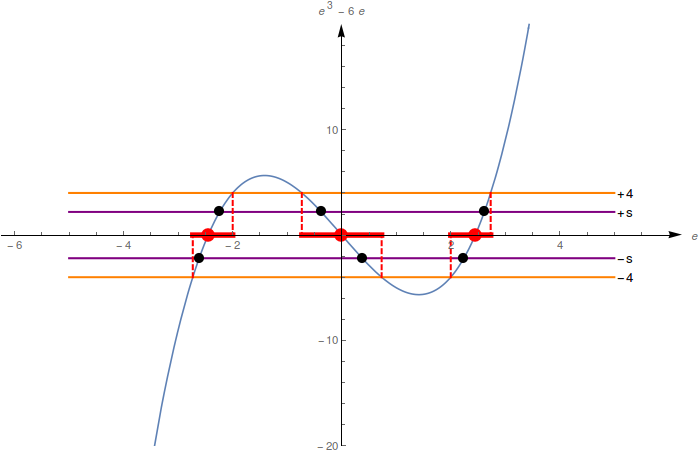
Figure 1. $p=1$, $q=3$: $E^{q}b_{p/q}(1/E)=E^{3}-6E$, the 3 horizontal red segments are the energy bands; the 3 red dots are the mid-band energies; the 6 black dots are the $\pm s$ energies.

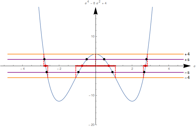
Figure 2. $p=1$, $q=4$: $E^{q}b_{p/q}(1/E)=E^{4}-8E^{2}+4$, the 4 horizontal red segments are the energy bands; the 4 red dots are the mid-band energies; the 8 black dots are the $\pm s$ energies.

It is quite straightforward to obtain for all $n$ and $q$ the mid-band trace formula

$${\rm Tr_{0}}H_{2\pi p/q}^{n}=\frac{n}{q}\sum_{\begin{subarray}{c}\ell_{1},\ell_{2},\ldots,\ell_{\lfloor q/2\rfloor}\geq 0\\ \ell_{1}+2\ell_{2}+\cdots+\lfloor q/2\rfloor\ell_{\lfloor q/2\rfloor}=n/2\end{subarray}}\frac{\binom{\ell_{1}+\ell_{2}+\cdots+\ell_{\lfloor q/2\rfloor}}{\ell_{1},\ell_{2},\ldots,\ell_{\lfloor q/2\rfloor}}}{\ell_{1}+\ell_{2}+\cdots+\ell_{\lfloor q/2\rfloor}}\prod_{j=1}^{\lfloor q/2\rfloor}a_{p/q}(2j)^{\ell_{j}}.$$ (14)

One can check that the Hofstadter trace (11) and the mid-band trace (14) indeed coincide provided that $q>n/2$ since then the summation index $k$ in (11) necessarily vanishes. A qualitative interpretation for this fact can stem from the classical picture of lattice walks contained in the quantum periodic cell of horizontal length $q$ (the lattice walk the farthest on the horizontal axis from the origin indeed goes to a distance $n/2$).

The mid-band trace (14) has a simple combinatorial interpretation: it is the sum of products of the $a_{p/q}(2j)^{\ell_{j}}$’s corresponding to partitions of $n$ in even integer parts of size $2j$ (no larger than $q$ since $a_{p/q}(2j)=0$ as soon as $q<2j$), i.e. $2\ell_{1}+4\ell_{2}+\cdots+2\lfloor q/2\rfloor\ell_{\lfloor q/2\rfloor}=n$, multiplied by the multinomial weight.

The generating function follows as

$$\sum_{n\geq 0,n\;{\rm even}}{\rm Tr_{0}}{H^{n}_{2\pi p/q}}z^{n}=1-\frac{zb^{\prime}_{p/q}(z)}{qb_{p/q}(z)},$$ (15)

which amounts to nothing else but (13), i.e. the $E_{r}(0)$’s are the roots of $E^{q}b_{b/q}(1/E)=0$. To see this rewrite

$$\sum_{n\geq 0,n\;{\rm even}}{\rm Tr_{0}}{H^{n}_{2\pi p/q}}z^{n} =\sum_{n\geq 0,n\;{\rm even}}{1\over q}\Big{(}\sum_{r=1}^{q}E_{r}^{n}(0)\Big{)}z^{n}={1\over q}\sum_{r=1}^{q}\sum_{n\geq 0,n\;{\rm even}}(zE_{r}(0))^{n}$$

$$={1\over q}\sum_{r=1}^{q}{1\over 1-z^{2}E_{r}^{2}(0)}={1\over 2q}\sum_{r=1}^{q}\Big{(}{1\over 1-zE_{r}(0)}+{1\over 1+zE_{r}(0)}\Big{)}={1\over q}\sum_{r=1}^{q}{1\over 1-zE_{r}(0)},$$

so that (15) becomes

$${1\over q}\sum_{r=1}^{q}{1\over 1-zE_{r}(0)}=1-\frac{zb^{\prime}_{p/q}(z)}{qb_{p/q}(z)}.$$ (16)

On the other hand (13) rewrites as

$$({1/z})^{q}b_{p/q}(z)=\prod_{r=1}^{q}({1/z}-E_{r}(0)),$$

that is

$$b_{p/q}(z)=\prod_{r=1}^{q}({1}-zE_{r}(0)),$$

so that

$$\big{(}\log(b_{p/q}(z))\big{)}^{\prime}=\sum_{r=1}^{q}{-E_{r}(0)\over{1}-zE_{r}(0)}={1\over z}\sum_{r=1}^{q}\Big{(}1-{1\over 1-zE_{r}(0)}\Big{)}$$

or

$${b_{p/q}(z)^{\prime}\over b_{p/q}(z)}={1\over z}\Big{(}q-\sum_{r=1}^{q}{1\over 1-zE_{r}(0)}\Big{)},$$

which is (16).

3.2. $\pm s$ trace formula:

More generally one can consider the $\pm s$ spectrum traces

$${\rm Tr_{\pm s}}{H^{n}_{2\pi p/q}}={1\over 2q}\Big{(}\sum_{r=1}^{q}E_{r}^{n}(s)+\sum_{r=1}^{q}E_{r}^{n}(-s)\Big{)}$$

taken on the $2q$ roots $E_{r}(s)$ and $E_{r}(-s)$ of

$$E^{q}b_{p/q}(1/E)=s\;{\rm and}\;E^{q}b_{p/q}(1/E)=-s$$ (17)

with $-4\leq s\leq 4$ since $-4\leq 2(\cos(qk_{x})+\cos(qk_{y}))\leq 4$ in (8). The mid-band spectrum is obtained for $s=0$, and the edge-band spectrum for $s=4$, of particular interest as well (see Figures 1 and 2).

Following the same line of reasoning as for the mid-band spectrum, one obtains the $\pm s$ spectrum traces generating function

$$\sum_{n\geq 0,n\;{\rm even}}{\rm Tr_{\pm s}}{H^{n}_{2\pi p/q}}z^{n} =1-\frac{z(b_{p/q}(z)-sz^{q})^{\prime}}{2q(b_{p/q}(z)-sz^{q})}-\frac{z(b_{p/q}(z)+sz^{q})^{\prime}}{2q(b_{p/q}(z)+sz^{q})}$$

$$=1-\frac{z(b^{2}_{p/q}(z)-s^{2}z^{2q})^{\prime}}{2q(b^{2}_{p/q}(z)-s^{2}z^{2q})}$$

$$=\Big{(}1-\frac{zb^{\prime}_{p/q}(z)}{qb_{p/q}(z)}\Big{)}{1\over 1-s^{2}(\frac{z^{q}}{b_{p/q}(z)})^{2}},$$ (18)

which rightly reduces to the mid-band case (15) when $s=0$. Again (18) is a mere rewriting of the $E_{r}(s)$’s and $E_{r}(-s)$’s being the roots of $E^{q}b_{p/q}(1/E)=\pm s$ in (17).

One has likewise the $\pm s$ trace formula

$${\rm Tr_{\pm s}}H_{2\pi p/q}^{n}=\frac{n}{q}\sum_{k\geq 0}\sum_{\begin{subarray}{c}\ell_{1},\ell_{2},\ldots,\ell_{\lfloor q/2\rfloor}\geq 0\\ \ell_{1}+2\ell_{2}+\cdots+\lfloor q/2\rfloor\ell_{\lfloor q/2\rfloor}=n/2-qk\end{subarray}}\frac{\binom{\ell_{1}+\ell_{2}+\cdots+\ell_{\lfloor q/2\rfloor}+2k}{\ell_{1},\ell_{2},\ldots,\ell_{\lfloor q/2\rfloor},2k}}{\ell_{1}+\ell_{2}+\cdots+\ell_{\lfloor q/2\rfloor}+2k}s^{2k}\prod_{j=1}^{\lfloor q/2\rfloor}a_{p/q}(2j)^{\ell_{j}}$$ (19)

which again reduces to the mid-band trace (14) when $s=0$. The combinatorial interpretation of (19) is again simple in terms of products of $s^{2}$ and of the $a_{p/q}(2j)$’s corresponding to all partitions of $n$ in even integer parts of size $2q$ and $2j$ respectively.

Again, as soon as $q>n/2$, the trace ${\rm Tr_{\pm s}}{H^{n}_{2\pi p/q}}$ in (19) does not depend on $s$ anymore and coincides with the Hofstadter trace (11) and, by the same token, with the mid-band trace (14).

3.3. Density of states:

One remarks next that the Hofstadter quantum trace ${\rm Tr}{H^{n}_{2\pi p/q}}$ in (11) can be recovered from the $\pm s$ spectrum trace ${\rm Tr_{\pm s}}{H^{n}_{2\pi p/q}}$ in (19) if one replaces $s^{2k}$ by ${2k\choose k}^{2}$. This replacement amounts to an integration of (19) over $s\in[-4,4]$ with a density of state $\rho(s)$

$$\int_{-4}^{4}{\rm Tr_{\pm s}}{H^{n}_{2\pi p/q}}\rho(s)ds={\rm Tr}{H^{n}_{2\pi p/q}}$$ (20)

such that

$$\int_{-4}^{4}s^{2k}\rho(s)ds={2k\choose k}^{2}$$ (21)

Clearly the free density of states on the 2d lattice,

$$\rho(s)=1/(2\pi^{2})K(1-s^{2}/16),$$ (22)

enforces (21): it is the density of states for the spectrum $s=2(\cos(qk_{x})+\cos(qk_{y}))$. Again, as soon as $q>n/2$, the integration in (20) becomes trivial, i.e. the identity.

For the generating function as well, which is given by

$$\int_{-4}^{4}\sum_{n}{\rm Tr_{\pm s}}{H^{n}_{2\pi p/q}}z^{n}\rho(s)ds=\sum_{n}{\rm Tr}{H^{n}_{2\pi p/q}}z^{n},$$

one uses (12), (18) and (22) so that

$$\int_{-4}^{4}\Big{(}1-\frac{z(b^{2}_{p/q}(z)-s^{2}z^{2q})^{\prime}}{2q(b^{2}_{p/q}(z)-s^{2}z^{2q})}\Big{)}{1\over 2\pi^{2}}K\left(1-{s^{2}\over 16}\right)ds=\Big{(}1-\frac{zb^{\prime}_{p/q}(z)}{qb_{p/q}(z)}\Big{)}\frac{2}{\pi}K\Big{(}16\Big{(}\frac{z^{q}}{b_{p/q}(z)}\Big{)}^{2}\Big{)}$$

has to be satisfied. After simplification this narrows down to

$$\int_{-4}^{4}{1\over 2\pi^{2}}K\left(1-{s^{2}\over 16}\right){1\over 1-s^{2}(\frac{z^{q}}{b_{p/q}(z)})^{2}}ds=\frac{2}{\pi}K\Big{(}16\Big{(}\frac{z^{q}}{b_{p/q}(z)}\Big{)}^{2}\Big{)},$$

i.e.

$$\int_{-4}^{4}K\left(1-{s^{2}\over 16}\right){1\over 1-s^{2}z^{2}}ds=4\pi{K(16z^{2})},$$

which is nothing but the complete elliptic integral of the first kind being the generating function for the square of the binomial coefficients, i.e. ${2\over\pi}K(16z^{2})=\sum_{k}{2k\choose k}^{2}\ z^{2k}$.

4. $\lambda\neq 2$ : point spectrum trace formula and density of states

All these considerations can be extended when $\lambda\neq 2$ to the almost Mathieu case (2) whose secular matrix is

$$m_{p/q}^{(\lambda)}(E,k_{x},k_{y})=\begin{pmatrix}\lambda\cos({k_{y}})-E&1&0&\cdots&0&e^{-i{qk_{x}}}\\ 1&\lambda\cos({k_{y}}+\frac{2\pi p}{q})-E&1&\cdots&0&0\\ 0&1&()&\cdots&0&0\\ \vdots&\vdots&\vdots&\ddots&\vdots&\vdots\\ 0&0&0&\cdots&()&1\\ e^{i{qk_{x}}}&0&0&\cdots&1&\lambda\cos({k_{y}}+(q-1)\frac{2\pi p}{q})-E\end{pmatrix}.$$ (23)

Thanks to the identity

$$\det(m_{p/q}^{(\lambda)}(E,k_{x},k_{y}))=\det(m_{p/q}^{(\lambda)}(E,0,0))-2(-1)^{q}(\cos(qk_{x})-1+({\lambda/2})^{q}(\cos(qk_{y})-1)),$$

the Schrödinger equation becomes

$$\det(m_{p/q}^{(\lambda)}(E,0,0))=2(-1)^{q}(\cos(qk_{x})-1+({\lambda/2})^{q}(\cos(qk_{y})-1)).$$ (24)

Again one introduces the polynomial $b_{p/q}^{(\lambda)}(z)$ and its coefficients $-a_{p/q}^{(\lambda)}(2j)$ (with $a_{p/q}^{(\lambda)}(0)=-1$)

$$b_{p/q}^{(\lambda)}(z)=-\sum_{j=0}^{[{q\over 2}]}a_{p/q}^{(\lambda)}(2j)z^{2j}$$ (25)

such that $\det(m_{p/q}^{(\lambda)}(E,0,0))$ rewrites as

$$\det(m_{p/q}^{(\lambda)}(E,0,0))+2(-1)^{q}(1+({\lambda/2})^{q})=(-1)^{q}E^{q}b_{p/q}^{(\lambda)}(1/E),$$ (26)

so that (24) becomes

$$E^{q}b_{p/q}^{(\lambda)}(1/E)=2(\cos(qk_{x})+({\lambda/2})^{q}\cos(qk_{y})).$$ (27)

In the appendix we show how to get a closed expression for the generalized Kreft coefficients $a_{p/q}^{(\lambda)}(2i)$’s in (25) following the steps of [3]. This procedure coalesces to

$$a_{p/q}^{(\lambda)}(2j) = (-1)^{j+1}\sum_{k_{1}=0}^{q-2j}\sum_{k_{2}=0}^{k_{1}}\ldots\sum_{k_{j}=0}^{k_{j-1}}\alpha_{p/q}^{(\lambda)}(k_{1}+2j-2)\overline{\alpha}_{p/q}^{(\lambda)}(k_{1}+2j-2)$$ (28)

$$\alpha_{p/q}^{(\lambda)}(k_{2}+2j-4)\overline{\alpha}_{p/q}^{(\lambda)}(k_{2}+2j-4)\ldots\alpha_{p/q}^{(\lambda)}(k_{j})\overline{\alpha}_{p/q}^{(\lambda)}(k_{j})$$

with for building blocks

$$\alpha_{p/q}^{(\lambda)}(k)\overline{\alpha}_{p/q}^{(\lambda)}(k),$$

where

$$\alpha_{p/q}^{(\lambda)}(k)=(\lambda/2)e^{-ik_{y}}\left(1-e^{{2i\pi(k+1)p\over q}}\right)$$

and

$$\overline{\alpha}_{p/q}^{(\lambda)}(k)=(\lambda/2)e^{ik_{y}}\left(1-({2/\lambda})^{2}e^{-{2i\pi(k+1)p\over q}}\right).$$

When $\lambda\neq 2$, even though $\overline{\alpha}_{p/q}^{(\lambda)}(k)$ is not anymore the complex conjugate of $\alpha_{p/q}^{(\lambda)}(k)$, it is still true that $a_{p/q}^{(\lambda)}(2j)$ in (28) is real. Indeed its imaginary part cancels because of

$$\sum_{k=1}^{q}\mathrm{e}^{\frac{2\mathrm{i}\pi kp}{q}j}=0$$

when $q>j$, being a sum of $j$-th powers of $q$-th roots of unity.

It follows that in the $\lambda\neq 2$ almost Mathieu case the $\pm s$ spectrum traces and their generating function are directly obtained by replacing in the Hofstadter $\pm s$ spectrum traces and generating functions (19) and (18) the $a_{p/q}(2j)$’s by the $a_{p/q}^{(\lambda)}(2j)$’s and so the polynomial $b_{p/q}(z)$ by $b_{p/q}^{(\lambda)}(z)$. This is due to the purely algebraic construction of these traces in terms of the $a_{p/q}(2j)$’s via the roots of (17) and therefore, in the $\lambda\neq 2$ case, the roots of

$$E^{q}b_{p/q}^{(\lambda)}(1/E)=\pm s$$

with $0\leq|s|\leq 2\big{(}1+(\lambda/2)^{q}\big{)}$, since from (27) necessarily $0\leq|2(\cos(qk_{x})+({\lambda/2})^{q}\cos(qk_{y}))|\leq 2\big{(}1+(\lambda/2)^{q}\big{)}$.

As stated in the introduction, one wishes to obtain a closed formula for the almost Mathieu quantum trace defined as

$${\rm Tr}\;(H_{2\pi p/q}^{(\lambda)})^{n}=\frac{1}{q}\int_{-\pi}^{\pi}\int_{-\pi}^{\pi}\frac{dk_{x}}{2\pi}\frac{dk_{y}}{2\pi}\sum_{r=1}^{q}(E_{r}^{(\lambda)}(k_{x},k_{y}))^{n},$$ (29)

where the $E_{r}^{(\lambda)}(k_{x},k_{y})$’s are the roots of (27). To do so, as in the Hofstadter case, one aims at integrating over $s\in[-2(1+(\lambda/2)^{q}),2(1+(\lambda/2)^{q})]$ the $\pm s$ spectrum trace with a density of state $\rho^{(\lambda)}(s)$

$$\int_{-2(1+(\lambda/2)^{q})}^{2(1+(\lambda/2)^{q})}{\rm Tr_{s}}({H^{(\lambda)}_{2\pi p/q}})^{n}\rho^{(\lambda)}(s)ds={\rm Tr}{(H^{(\lambda)}_{2\pi p/q})^{n}}$$

which has necessarily to be such that

$$\int_{-2(1+(\lambda/2)^{q})}^{2(1+(\lambda/2)^{q})}s^{2k}\rho^{(\lambda)}(s)ds={2k\choose k}\sum_{k_{1}=0}^{k}{k\choose k_{1}}^{2}(\lambda/2)^{2qk_{1}}$$ (30)

in analogy to (21). A derivation of $\rho^{(\lambda)}(s)$ enforcing (30) is given in the appendix. This density of states amounts to a $\lambda$-deformation of $\rho(s)$ in (22) for the 2d lattice spectrum $s=2(\cos(qk_{x})+(\lambda/2)^{q}\cos(qk_{y}))$.

Putting all the steps above together, namely in (19) replacing both the $a_{p/q}(2j)$’s by the $a_{p/q}^{(\lambda)}(2j)$’s and $s^{2k}$ by ${2k\choose k}\sum_{k_{1}=0}^{k}{k\choose k_{1}}^{2}(\lambda/2)^{2qk_{1}}$, the almost Mathieu operator quantum trace (29) ends up as

$${\rm Tr}\;(H_{2\pi p/q}^{(\lambda)})^{n}= \frac{n}{q}\sum_{k\geq 0}\sum_{\begin{subarray}{c}\ell_{1},\ell_{2},\ldots,\ell_{\lfloor q/2\rfloor}\geq 0\\ \ell_{1}+2\ell_{2}+\cdots+\lfloor q/2\rfloor\ell_{\lfloor q/2\rfloor}=n/2-qk\end{subarray}}\frac{\binom{\ell_{1}+\ell_{2}+\cdots+\ell_{\lfloor q/2\rfloor}+2k}{\ell_{1},\ell_{2},\ldots,\ell_{\lfloor q/2\rfloor},2k}}{\ell_{1}+\ell_{2}+\cdots+\ell_{\lfloor q/2\rfloor}+2k}{2k\choose k}\sum_{k_{1}=0}^{k}{k\choose k_{1}}^{2}(\lambda/2)^{2qk_{1}}$$ (31)

$$\prod_{j=1}^{\lfloor q/2\rfloor}a_{p/q}^{(\lambda)}(2j)^{\ell_{j}},$$

which is a $\lambda$-deformation of the quantum Hofstadter trace (11).

One also gets the generating function that generalizes (12)

$$\sum_{n\geq 0}Z_{n}^{(\lambda)}(e^{2i\pi p/q})z^{n}=\Big{(}1-\frac{z(b_{p/q}^{(\lambda)}(z))^{\prime}}{qb_{p/q}^{(\lambda)}(z)}\Big{)}\sum_{k\geq 0}\binom{2k}{k}\sum_{k_{1}=0}^{k}\binom{k}{k_{1}}^{2}(\lambda/2)^{2qk_{1}}\Big{(}\frac{z^{q}}{b_{p/q}^{(\lambda)}(z)}\Big{)}^{2k},$$ (32)

where $\sum_{k\geq 0}\binom{2k}{k}\sum_{k_{1}=0}^{k}\binom{k}{k_{1}}^{2}(\lambda/2)^{2qk_{1}}x^{k}$ can be viewed as a $\lambda$-deformation of the complete elliptic integral of the first kind $\frac{2}{\pi}K(16x)=\sum_{k\geq 0}\binom{2k}{k}^{2}x^{k}$.

Note finally that one can check that the Aubry duality [9]

$${\rm Tr}\;(H_{2\pi p/q}^{(\lambda)})^{n}=({\lambda\over 2})^{n}{\rm Tr}\;(H_{2\pi p/q}^{(4/\lambda)})^{n},$$ (33)

holds, as it should. This happens because the generalized Kreft coefficients (28) obey themselves the duality

$$a_{p/q}^{(\lambda)}(2j)=({\lambda\over 2})^{2j}\;a_{p/q}^{(4/\lambda)}(2j)$$ (34)

which follows from

$${\rm Re}\left(\alpha_{p/q}^{(\lambda)}(k)\overline{\alpha}_{p/q}^{(\lambda)}(k)\right)=\Big{(}{\lambda\over 2}\Big{)}^{2}\;{\rm Re}\left(\alpha_{p/q}^{(4/\lambda)}(k)\overline{\alpha}_{p/q}^{(4/\lambda)}(k)\right)$$

(only the real part is needed here since $a_{p/q}^{(\lambda)}(2j)$ is real). The duality (33) then follows from (31) and the duality (34)

$${\rm Tr}\;(H_{2\pi p/q}^{(\lambda)})^{n} =\frac{n}{q}\sum_{k\geq 0}\sum_{\begin{subarray}{c}\ell_{1},\ell_{2},\ldots,\ell_{\lfloor q/2\rfloor}\geq 0\\ \ell_{1}+2\ell_{2}+\cdots+\lfloor q/2\rfloor\ell_{\lfloor q/2\rfloor}=n/2-qk\end{subarray}}\frac{{2k\choose k}\sum_{k_{1}=0}^{k}{k\choose k_{1}}^{2}(\lambda/2)^{2qk_{1}}\binom{\ell_{1}+\ell_{2}+\cdots+\ell_{\lfloor q/2\rfloor}+2k}{\ell_{1},\ell_{2},\ldots,\ell_{\lfloor q/2\rfloor},2k}}{\ell_{1}+\ell_{2}+\cdots+\ell_{\lfloor q/2\rfloor}+2k}$$

$$\left(\lambda/2\right)^{\sum_{j=1}^{\lfloor q/2\rfloor}2jl_{j}}\prod_{j=1}^{\lfloor q/2\rfloor}a_{p/q}^{(4/\lambda)}(2j)^{\ell_{j}}$$

$$=\frac{n}{q}\sum_{k\geq 0}\sum_{\begin{subarray}{c}\ell_{1},\ell_{2},\ldots,\ell_{\lfloor q/2\rfloor}\geq 0\\ \ell_{1}+2\ell_{2}+\cdots+\lfloor q/2\rfloor\ell_{\lfloor q/2\rfloor}=n/2-qk\end{subarray}}\frac{{2k\choose k}\sum_{k_{1}=0}^{k}{k\choose k_{1}}^{2}(\lambda/2)^{2qk_{1}}\binom{\ell_{1}+\ell_{2}+\cdots+\ell_{\lfloor q/2\rfloor}+2k}{\ell_{1},\ell_{2},\ldots,\ell_{\lfloor q/2\rfloor},2k}}{\ell_{1}+\ell_{2}+\cdots+\ell_{\lfloor q/2\rfloor}+2k}$$

$$\left(\lambda/2\right)^{n-2qk}\prod_{j=1}^{\lfloor q/2\rfloor}a_{p/q}^{(4/\lambda)}(2j)^{\ell_{j}}$$

$$=\left(\lambda/2\right)^{n}\frac{n}{q}\sum_{k\geq 0}\sum_{\begin{subarray}{c}\ell_{1},\ell_{2},\ldots,\ell_{\lfloor q/2\rfloor}\geq 0\\ \ell_{1}+2\ell_{2}+\cdots+\lfloor q/2\rfloor\ell_{\lfloor q/2\rfloor}=n/2-qk\end{subarray}}\frac{{2k\choose k}\sum_{k_{1}=0}^{k}{k\choose k_{1}}^{2}(2/\lambda)^{2qk-2qk_{1}}\binom{\ell_{1}+\ell_{2}+\cdots+\ell_{\lfloor q/2\rfloor}+2k}{\ell_{1},\ell_{2},\ldots,\ell_{\lfloor q/2\rfloor},2k}}{\ell_{1}+\ell_{2}+\cdots+\ell_{\lfloor q/2\rfloor}+2k}$$

$$\prod_{j=1}^{\lfloor q/2\rfloor}a_{p/q}^{(4/\lambda)}(2j)^{\ell_{j}}$$

$$\stackrel{{\scriptstyle\text{$k^{\prime}_{1}=k-k_{1}$}}}{{=}}\left(\lambda/2\right)^{n}\frac{n}{q}\sum_{k\geq 0}\sum_{\begin{subarray}{c}\ell_{1},\ell_{2},\ldots,\ell_{\lfloor q/2\rfloor}\geq 0\\ \ell_{1}+2\ell_{2}+\cdots+\lfloor q/2\rfloor\ell_{\lfloor q/2\rfloor}=n/2-qk\end{subarray}}\frac{{2k\choose k}\sum_{k^{\prime}_{1}=0}^{k}{k\choose k^{\prime}_{1}}^{2}(2/\lambda)^{2qk^{\prime}_{1}}\binom{\ell_{1}+\ell_{2}+\cdots+\ell_{\lfloor q/2\rfloor}+2k}{\ell_{1},\ell_{2},\ldots,\ell_{\lfloor q/2\rfloor},2k}}{\ell_{1}+\ell_{2}+\cdots+\ell_{\lfloor q/2\rfloor}+2k}$$

$$\prod_{j=1}^{\lfloor q/2\rfloor}a_{p/q}^{(4/\lambda)}(2j)^{\ell_{j}}=\left(\lambda/2\right)^{n}{\rm Tr}\;(H_{2\pi p/q}^{(4/\lambda)})^{n}$$

.

5. Conclusion

One has obtained the $\lambda$-deformation of the quantum trace (11) in the form of (31). Both trace formulae have a similar structure, with clearly (31), the almost Mathieu case, reducing when $\lambda=2$ to (11), the Hofstadter case. Going back for a moment to random walks on a lattice, it would certainly be interesting to look at possible interpretations of (31) in the context of asymmetric paths with unequal probabilities on the horizontal and vertical axis.

On the other hand, our results are directly relevant for problems related to Calabi-Yau geometry. A recent work [10] indicates that there exists in the rational case a relation between the almost Mathieu operator and the relativistic Toda lattice. As pointed out in section 2 of [10], there is an invariance under the modular double operation exchanging $\gamma=2\pi p/q$ and $\tilde{\gamma}=2\pi q/p$ (respectively $\hbar$ and $\tilde{\hbar}$ in the notations of [10]) of the relativistic relative 2-body Toda Hamiltonian

$$H=\lambda(e^{p}+e^{-p})+e^{x}+e^{-x},\quad[x,p]=i\gamma$$ (35)

where, in [10], $\lambda$ is denoted as $R^{2}$. The eigenvalues $E$ and $\tilde{E}$ corresponding to $\gamma$ and $\tilde{\gamma}$ satisfy the polynomial identity $P_{p/q}(E)=P_{q/p}(\tilde{E})$ where $P_{p/q}(E)$ is a polynomial of degree $q$ (see $2.19$ in [10]). Now this polynomial is identical to the polynomial $E^{q}b_{p/q}^{(\lambda)}(1/E)$ introduced in (25),(26) which encodes the $k_{x},k_{y}$-independent part of the determinant of the almost Mathieu Schrodinger equation encapsulated in $m_{p/q}^{(\lambda)}(E,k_{x},k_{y})$. In the present work we have precisely obtained in (28) a closed expression for these polynomials in terms of the generalized Kreft coefficients.

It would certainly be rewarding to see if (28) can bring any pertinent information related to the various qestions raised in [10], in particlar regarding the quantum A-period for the modulus of the underlying Calabi-Yau geometry. Finally, in the context of the Hofstadter model itself, the true role of the double modular transformation $\gamma\to\tilde{\gamma}$ remains to be elucidated.

6. Acknowledgements

S.W. was supported by the National Research Foundation of South Africa, grant number 96236. S.O. would like to thank S. Nechaev for drawing his attention to [10].

7. Appendix

7.1. Kreft’s coefficients construction:

Following Kreft [3] we show how to get a closed expression for the polynomial (26), i.e. for the Kreft coefficients $a_{p/q}^{(\lambda)}(2j)$ in $b_{p/q}^{(\lambda)}(z)=-\sum_{j=0}^{[{q\over 2}]}a_{p/q}^{(\lambda)}(2j)z^{2j}$ as defined in (25).

7.1.1. $\lambda=2$:

One aims at transforming the matrix $m_{p/q}\left(E,k_{x},k_{y}\right)$ in (3) into a tridiagonal one by an appropriate change of basis. First, let us do the change of basis

$$m_{1}=\begin{pmatrix}1&0&0&\cdots&0&0\\ 0&e^{ik_{x}}&0&\cdots&0&0\\ 0&0&e^{i2k_{x}}&\cdots&0&0\\ \vdots&\vdots&\vdots&\ddots&\vdots&\vdots\\ 0&0&0&\cdots&e^{i(q-2)k_{x}}&0\\ 0&0&0&\cdots&0&e^{i(q-1)k_{x}}\\ \end{pmatrix}$$

so that $m_{p/q}\left(E,k_{x},k_{y}\right)$ rewrites as

$$m^{-1}_{1}m_{p/q}\left(E,k_{x},k_{y}\right)m_{1}=\begin{pmatrix}2\cos({k_{y}})-E&e^{ik_{x}}&0&\cdots&0&e^{-ik_{x}}\\ e^{-ik_{x}}&2\cos({k_{y}}+\frac{2\pi p}{q})-E&e^{ik_{x}}&\cdots&0&0\\ 0&e^{-ik_{x}}&()&\cdots&0&0\\ \vdots&\vdots&\vdots&\ddots&\vdots&\vdots\\ 0&0&0&\cdots&()&e^{ik_{x}}\\ e^{ik_{x}}&0&0&\cdots&e^{-ik_{x}}&2\cos({k_{y}}+(q-1)\frac{2\pi p}{q})-E\\ \end{pmatrix}$$

In this new basis the Schrödinger equation (1) with ${\Phi}_{m+q}=e^{iqk_{x}}{\Phi}_{m}$ becomes

$$e^{ik_{x}}\Phi_{m+1}^{\prime}+e^{-ik_{x}}\Phi_{m-1}^{\prime}+2\cos\left(k_{y}+\gamma m\right)\Phi_{m}^{\prime}=E\Phi_{m}^{\prime},\quad\Phi_{m+q}^{\prime}=\Phi_{m}^{\prime}$$

Then let us do a second change of basis $m_{2}$ with matrix element

$$m_{jk}=\frac{1}{\sqrt{q}}(-1)^{pk}e^{\frac{2i\pi p}{q}\left(jk-k^{2}/2\right)},\quad k,j\in\{0,1,\ldots,q-1\}.$$

Putting together $m_{1}$ and $m_{2}$ amounts to the change of basis $m_{1}m_{2}$ with matrix element $e^{ikk_{x}}m_{jk}=e^{ikk_{x}}\frac{1}{\sqrt{q}}(-1)^{pk}e^{\frac{2i\pi p}{q}\left(jk-k^{2}/2\right)}$

$$(m_{1}m_{2})^{-1}m_{p/q}\left(E,k_{x},k_{y}\right)m_{1}m_{2}=\begin{pmatrix}-E&\alpha_{p/q}(0)&0&\cdots&0&\overline{\alpha}_{p/q}(q-1)\\ \overline{\alpha}_{p/q}(0)&-E&\alpha_{p/q}(1)&\cdots&0&0\\ 0&\overline{\alpha}_{p/q}(1)&-E&\cdots&0&0\\ \vdots&\vdots&\vdots&\ddots&\vdots&\vdots\\ 0&0&0&\cdots&-E&\alpha_{p/q}({q-2})\\ \alpha_{p/q}({q-1})&0&0&\cdots&\overline{\alpha}_{p/q}({q-2})&-E\\ \end{pmatrix}$$ (36)

where $\alpha_{p/q}(k)=e^{-ik_{y}}-(-1)^{(p+1)}e^{\frac{2i\pi p}{q}(k+1/2)+ik_{x}}$, $\overline{\alpha}_{p/q}(k)$ is its complex conjugate and accordingly

$$\alpha_{p/q}(m){\tilde{\Phi}}_{m+1}+\overline{\alpha}_{p/q}(m-1){\tilde{\Phi}}_{m-1}=E{\tilde{\Phi}}_{m},\quad{\tilde{\Phi}}_{m+q}={\tilde{\Phi}}_{m}$$ (37)

Both corners $\alpha_{p/q}({q-1})$ and $\overline{\alpha}_{p/q}({q-1})$ in the matrix (36) can be cancelled if $e^{i(k_{x}+k_{y})}=(-1)^{(p+1)}e^{-\frac{2i\pi p}{q}(q-1+1/2)}=(-1)^{(p+1)}e^{\frac{i\pi p}{q}}$, i.e. if $k_{x}+k_{y}=\pi(p+1)+\frac{\pi p}{q}$. The matrix is then tridiagonal with a determinant in (4) equal to $(-1)^{q}E^{q}b_{p/q}(1/E)$, since the trigonometric part vanishes as well: indeed

$$\cos(qk_{x})+\cos(qk_{y}) =2\cos({q(k_{x}+k_{y})\over 2})\cos({q(k_{x}-k_{y})\over 2})$$

$$=2\cos({\pi(p+q(p+1))\over 2})\cos({q(k_{x}-k_{y})\over 2})$$

$$=0$$

due to $p+q(p+1)$ being always odd since $p$ and $q$ are co-prime.

One gets the tridiagonal matrix

$$\begin{pmatrix}-E&\alpha_{p/q}(0)&0&\cdots&0&0\\ \overline{\alpha}_{p/q}(0)&-E&\alpha_{p/q}(1)&\cdots&0&0\\ 0&\overline{\alpha}_{p/q}(1)&-E&\cdots&0&0\\ \vdots&\vdots&\vdots&\ddots&\vdots&\vdots\\ 0&0&0&\cdots&-E&\alpha_{p/q}({q-2)}\\ 0&0&0&\cdots&\overline{\alpha}_{p/q}({q-2})&-E\\ \end{pmatrix}$$ (38)

where $\alpha_{p/q}(k)$, using $e^{i(k_{x}+k_{y})}=(-1)^{(p+1)}e^{\frac{i\pi p}{q}}$, has simplified to $\alpha_{p/q}(k)=e^{-ik_{y}}(1-e^{\frac{2i\pi(k+1)p}{q}})$. The matrix (38) does not depend anymore on $k_{x}$ nor $k_{y}$ and its determinant satisfies a recursion (see [3]) leading respectively to the Kreft polynomial and Kreft coefficients (7) and (9).

7.1.2. $\lambda\neq 2$:

One uses the same method as above to find a closed expression for the polynomial $b^{(\lambda)}_{p/q}(1/E)$, namely transform the matrix $m_{p/q}^{(\lambda)}\left(E,k_{x},k_{y}\right)$ in (23) into a tridiagonal one. To do so use the same change of basis $m_{1}m_{2}$ as above so that

$$(m_{1}m_{2})^{-1}m^{(\lambda)}_{p/q}\left(E,k_{x},k_{y},\right)m_{1}m_{2}=\begin{pmatrix}-E&\alpha_{p/q}^{(\lambda)}(0)&0&\cdots&0&\overline{\alpha}_{p/q}^{(\lambda)}({q-1})\\ \overline{\alpha}_{p/q}^{(\lambda)}(0)&-E&\alpha_{p/q}^{(\lambda)}(1)&\cdots&0&0\\ 0&\overline{\alpha}_{p/q}^{(\lambda)}(1)&-E&\cdots&0&0\\ \vdots&\vdots&\vdots&\ddots&\vdots&\vdots\\ 0&0&0&\cdots&-E&\alpha_{p/q}^{(\lambda)}({q-2})\\ \alpha_{p/q}^{(\lambda)}({q-1})&0&0&\cdots&\overline{\alpha}_{p/q}^{(\lambda)}({q-2})&-E\\ \end{pmatrix}$$ (39)

with $\alpha_{p/q}^{(\lambda)}(k)=({\lambda}/{2})e^{-ik_{y}}-(-1)^{p+1}e^{i\frac{2\pi p}{q}(k+1/2)+ik_{x}}$ and $\overline{\alpha}_{p/q}^{(\lambda)}(k)$ its complex conjugate. Moreover, we have a resulting Schrödinger equation identical to (37) provided that $\alpha_{p/q}(k)$ is replaced with $\alpha_{p/q}^{(\lambda)}(k)$.

Contrary to the Hofstadter case $\lambda=2$, both corners ${\alpha_{p/q}^{(\lambda)}({q-1})}$ and $\overline{\alpha}_{p/q}^{(\lambda)}({q-1})$ in the matrix (39) cannot simultaneously vanish. One can still choose to have the lower left corner ${\alpha_{p/q}^{(\lambda)}({q-1})}$ to vanish: this amounts to $e^{i(k_{x}+k_{y})}=(-1)^{p+1}({\lambda}/{2})e^{-i\frac{2\pi p}{q}(q-1+1/2)}=(-1)^{p+1}({\lambda}/{2})e^{\frac{i\pi p}{q}}$, which can only be achieved for a complex $k_{x}+k_{y}$ (namely $k_{x}+k_{y}=-i\log(\lambda/2)+\frac{\pi p}{q}+\pi(p+1)$), so that $e^{-i(k_{x}+k_{y})}=(-1)^{p+1}({2}/{\lambda})e^{-\frac{i\pi p}{q}}$. The matrix (39) then becomes

$$\begin{pmatrix}-E&\alpha_{p/q}^{(\lambda)}(0)&0&\cdots&0&\overline{\alpha}_{p/q}^{(\lambda)}({q-1})\\ \overline{\alpha}_{p/q}^{(\lambda)}(0)&-E&\alpha_{p/q}^{(\lambda)}(1)&\cdots&0&0\\ 0&\overline{\alpha}_{p/q}^{(\lambda)}(1)&-E&\cdots&0&0\\ \vdots&\vdots&\vdots&\ddots&\vdots&\vdots\\ 0&0&0&\cdots&-E&\alpha_{p/q}^{(\lambda)}({q-2})\\ 0&0&0&\cdots&\overline{\alpha}_{p/q}^{(\lambda)}({q-2})&-E\\ \end{pmatrix}$$ (40)

where $\alpha_{p/q}^{(\lambda)}(k)$ and $\overline{\alpha}_{p/q}^{(\lambda)}(k)$ have simplified to $\alpha_{p/q}^{(\lambda)}(k)=({\lambda}/{2})e^{-ik_{y}}(1-e^{\frac{2i\pi(k+1)p}{q}})$ and $\overline{\alpha}_{p/q}^{(\lambda)}(k)=({\lambda}/{2})e^{ik_{y}}(1-({2}/{\lambda})^{2}e^{-\frac{2i\pi(k+1)p}{q}})$. Note that $\overline{\alpha}_{p/q}^{(\lambda)}(k)$ is not anymore the complex conjugate of $\alpha_{p/q}^{(\lambda)}(k)$.

By expanding the determinant of (40) with respect to the elements of the first row

$$\begin{vmatrix}-E&\alpha_{p/q}^{(\lambda)}(0)&0&\cdots&0&\overline{\alpha}_{p/q}^{(\lambda)}({q-1})\\ \overline{\alpha}_{p/q}^{(\lambda)}(0)&-E&\alpha_{p/q}^{(\lambda)}(1)&\cdots&0&0\\ 0&\overline{\alpha}_{p/q}^{(\lambda)}(1)&-E&\cdots&0&0\\ \vdots&\vdots&\vdots&\ddots&\vdots&\vdots\\ 0&0&0&\cdots&-E&\alpha_{p/q}^{(\lambda)}({q-2})\\ 0&0&0&\cdots&\overline{\alpha}_{p/q}^{(\lambda)}({q-2})&-E\end{vmatrix}=-E\begin{vmatrix}-E&\alpha_{p/q}^{(\lambda)}(1)&\cdots&0&0\\ \overline{\alpha}_{p/q}^{(\lambda)}(1)&-E&\cdots&0&0\\ \vdots&\vdots&\ddots&\vdots&\vdots\\ 0&0&\cdots&-E&\alpha_{p/q}^{(\lambda)}({q-2})\\ 0&0&\cdots&\overline{\alpha}_{p/q}^{(\lambda)}({q-2})&-E\end{vmatrix}$$

$$-\alpha_{p/q}^{(\lambda)}(0)\overline{\alpha}_{p/q}^{(\lambda)}(0)\begin{vmatrix}-E&\alpha_{p/q}^{(\lambda)}(2)&\cdots&0&0\\ \overline{\alpha}_{p/q}^{(\lambda)}(2)&-E&\cdots&0&0\\ \vdots&\vdots&\ddots&\vdots&\vdots\\ 0&0&\cdots&-E&\alpha_{p/q}^{(\lambda)}({q-2})\\ 0&0&\cdots&\overline{\alpha}_{p/q}^{(\lambda)}({q-2})&-E\end{vmatrix}$$

$$+(-1)^{q+1}\overline{\alpha}_{p/q}^{(\lambda)}({q-1})\begin{vmatrix}\overline{\alpha}_{p/q}^{(\lambda)}(0)&-E&\alpha_{p/q}^{(\lambda)}(1)&\cdots&0&0\\ 0&\overline{\alpha}_{p/q}^{(\lambda)}(1)&-E&\cdots&0&0\\ \vdots&\vdots&\vdots&\ddots&\vdots&\vdots\\ 0&0&0&\cdots&\overline{\alpha}_{p/q}^{(\lambda)}({q-3})&-E\\ 0&0&0&\cdots&0&\overline{\alpha}_{p/q}^{(\lambda)}({q-2})\end{vmatrix}$$ (41)

it is immediate to see that the part that depends on $k_{x}$ or $k_{y}$ can only come from the last term of (41), i.e. from the upper right corner $\overline{\alpha}_{p/q}^{(\lambda)}({q-1})$. Therefore to get the desired $k_{x},k_{y}$-independent polynomial $E^{q}b^{(\lambda)}_{p/q}(1/E)$, all that is needed is the determinant of the tridiagonal matrix

$$\begin{pmatrix}-E&\alpha_{p/q}^{(\lambda)}(0)&0&\cdots&0&0\\ \overline{\alpha}_{p/q}^{(\lambda)}(0)&-E&\alpha_{p/q}^{(\lambda)}(1)&\cdots&0&0\\ 0&\overline{\alpha}_{p/q}^{(\lambda)}(1)&-E&\cdots&0&0\\ \vdots&\vdots&\vdots&\ddots&\vdots&\vdots\\ 0&0&0&\cdots&-E&\alpha_{p/q}^{(\lambda)}({q-2})\\ 0&0&0&\cdots&\overline{\alpha}_{p/q}^{(\lambda)}({q-2})&-E\\ \end{pmatrix}$$

which finally yields the $\lambda\neq 2$ Kreft polynomial and Kreft coefficients (26) and (28).

7.2. Density of states $\rho^{(\lambda)}(s)$:

To simplify the notations let us denote in this section $(\lambda/2)^{q}$ by $\tilde{\lambda}$. Knowing that

$$\int_{-4}^{4}\rho(s)s^{2k}\,ds=\binom{2k}{k}^{2}$$

for $\rho(s)=(2\pi^{2})^{-1}K(1-s^{2}/16)$, where $K$ denotes the elliptic integral, we would like to determine a function $\rho^{(\lambda)}(s)$ such that

$$\int_{-2(1+\tilde{\lambda})}^{2(1+\tilde{\lambda})}\rho^{(\lambda)}(s)s^{2k}\,ds=\binom{2k}{k}\sum_{k_{1}=0}^{k}\binom{k}{k_{1}}^{2}\tilde{\lambda}^{2k_{1}}$$

as in (30). The special case $\tilde{\lambda}=1$ clearly corresponds to the aforementioned formula.

We interpret the desired function $\rho^{(\lambda)}(s)$ as the density of a random variable with support $[-2(1+\tilde{\lambda}),2(1+\tilde{\lambda})]$ that is symmetric (so that the odd-order moments are $0$) and has $2k$-th moment

$$M_{2k}=\binom{2k}{k}\sum_{k_{1}=0}^{k}\binom{k}{k_{1}}^{2}\tilde{\lambda}^{2k_{1}}.$$

The moment generating function associated with this random variable is

$$\sum_{k=0}^{\infty}\frac{M_{2k}}{(2k)!}x^{2k} =\sum_{k=0}^{\infty}\binom{2k}{k}\sum_{k_{1}=0}^{k}\binom{k}{k_{1}}^{2}\tilde{\lambda}^{2k_{1}}\frac{x^{2k}}{(2k)!}$$

$$=\sum_{k_{1}=0}^{\infty}\sum_{k=k_{1}}^{\infty}\binom{2k}{k}\binom{k}{k_{1}}^{2}\tilde{\lambda}^{2k_{1}}\frac{x^{2k}}{(2k)!}$$

$$=\sum_{k_{1}=0}^{\infty}\frac{\tilde{\lambda}^{2k_{1}}}{k_{1}!^{2}}\sum_{k=k_{1}}^{\infty}\frac{1}{(k-k_{1})!^{2}}x^{2k}$$

$$=\sum_{k_{1}=0}^{\infty}\frac{\tilde{\lambda}^{2k_{1}}}{k_{1}!^{2}}\sum_{j=0}^{\infty}\frac{1}{j!^{2}}x^{2(k_{1}+j)}$$

$$=\sum_{k_{1}=0}^{\infty}\frac{\tilde{\lambda}^{2k_{1}}x^{2k_{1}}}{k_{1}!^{2}}\sum_{j=0}^{\infty}\frac{x^{2j}}{j!^{2}}$$

$$=I(2\tilde{\lambda}x)I(2x),$$

where $I$ denotes the $0$-th order modified Bessel function of the first kind. Thus the random variable whose density $\rho^{({\lambda})}(s)$ we would like to determine is the convolution of two random variables with moment generating functions $I(2\tilde{\lambda}x)$ and $I(2x)$ respectively.

Now note that $I(2x)$ is exactly the moment generating function of an arcsine distribution on the interval $[-2,2]$:

$$\int_{-2}^{2}\frac{e^{sx}}{\pi\sqrt{4-s^{2}}}\,ds=I(2x),$$

and likewise $I(2\tilde{\lambda}x)$ is the moment generating function of an arcsine distribution on the interval $[-2\tilde{\lambda},2\tilde{\lambda}]$:

$$\int_{-2\tilde{\lambda}}^{2\tilde{\lambda}}\frac{e^{sx}}{\pi\sqrt{4\tilde{\lambda}^{2}-s^{2}}}\,ds=I(2\tilde{\lambda}x).$$

Therefore $\rho^{({\lambda})}(s)$ must be the convolution of the two densities $h_{1}(s)=(\pi\sqrt{4-s^{2}})^{-1}$ ($s\in[-2,2]$, otherwise $h_{1}(s)=0$) and $h_{2}(s)=(\pi\sqrt{4\tilde{\lambda}^{2}-s^{2}})^{-1}$ ($s\in[-2\tilde{\lambda},2\tilde{\lambda}]$, otherwise $h_{2}(s)=0$), which is

$$\rho^{(\lambda)}(s)=\int_{-\infty}^{\infty}h_{1}(s-t)h_{2}(t)\,dt.$$

This reduces to several different cases:

• Case 1: $\tilde{\lambda}>1$

  1. if $s<-2-2\tilde{\lambda}$ or $s>2+2\tilde{\lambda}$, then $\rho^{(\lambda)}(s)=0$;

  2. if $-2-2\tilde{\lambda}\leq s<2-2\tilde{\lambda}$, then

     $$\rho^{(\lambda)}(s)=\pi^{-2}\int_{-2\tilde{\lambda}}^{s+2}\frac{1}{\sqrt{(4-(s-t)^{2})(4\tilde{\lambda}^{2}-t^{2})}}\,dt;$$

  3. if $2-2\tilde{\lambda}\leq s\leq 2\tilde{\lambda}-2$, then

     $$\rho^{(\lambda)}(s)=\pi^{-2}\int_{s-2}^{s+2}\frac{1}{\sqrt{(4-(s-t)^{2})(4\tilde{\lambda}^{2}-t^{2})}}\,dt;$$

  4. if $2\tilde{\lambda}-2<s\leq 2\tilde{\lambda}+2$, then

     $$\rho^{(\lambda)}(s)=\pi^{-2}\int_{s-2}^{2\tilde{\lambda}}\frac{1}{\sqrt{(4-(s-t)^{2})(4\tilde{\lambda}^{2}-t^{2})}}\,dt.$$

• Case 2: $0<\tilde{\lambda}<1$

  1. if $s<-2-2\tilde{\lambda}$ or $s>2+2\tilde{\lambda}$, then $\rho^{(\lambda)}(s)=0$;

  2. if $-2-2\tilde{\lambda}\leq s<2\tilde{\lambda}-2$, then

     $$\rho^{(\lambda)}(s)=\pi^{-2}\int_{-2\tilde{\lambda}}^{s+2}\frac{1}{\sqrt{(4-(s-t)^{2})(4\tilde{\lambda}^{2}-t^{2})}}\,dt;$$

  3. if $2\tilde{\lambda}-2\leq s\leq 2-2\tilde{\lambda}$, then

     $$\rho^{(\lambda)}(s)=\pi^{-2}\int_{-2\tilde{\lambda}}^{2\tilde{\lambda}}\frac{1}{\sqrt{(4-(s-t)^{2})(4\tilde{\lambda}^{2}-t^{2})}}\,dt;$$

  4. if $2-2\tilde{\lambda}<s\leq 2\tilde{\lambda}+2$, then

     $$\rho^{(\lambda)}(s)=\pi^{-2}\int_{s-2}^{2\tilde{\lambda}}\frac{1}{\sqrt{(4-(s-t)^{2})(4\tilde{\lambda}^{2}-t^{2})}}\,dt.$$

7.3. Eq. (32) can be directly obtained as in [1]:

In order to reproduce from the lattice walks formulation in [1] the results obtained above for $\lambda\neq 2$, all that is needed is to set in the generating function $A(x_{1},x_{2},y_{1},y_{2},{\textsc{q}})$ (defined in eq.(10) of [1]) $x_{1}\rightarrow zx$, $x_{2}\rightarrow z/x$, $y_{1}\rightarrow(\lambda/2)zy$ and $y_{2}\rightarrow(\lambda/2)z/y$ and look as in [1] at the coefficients with vanishing exponents in $x$ and $y$ (i.e. $m_{1}-m_{2}=0$ and $l_{1}-l_{2}=0$) and exponent $n$ in $z$ (i. e., $m_{1}+m_{2}+l_{1}+l_{2}=n$)

$$\left[x^{0}y^{0}\right]A\left(zx,z/x,(\lambda/2)zy,(\lambda/2)z/y\right)=\left[x^{0}y^{0}\right]\frac{\begin{vmatrix}1&-z/x&0&\cdots&0&-zx\\ 1&c^{(\lambda)}_{1}&-z/x&\cdots&0&0\\ 1&-zx&c^{(\lambda)}_{2}&\cdots&0&0\\ \vdots&\vdots&\vdots&\ddots&\vdots&\vdots\\ 1&0&0&\cdots&c^{(\lambda)}_{q-2}&-z/x\\ 1&0&0&\cdots&-zx&c^{(\lambda)}_{q-1}\\ \end{vmatrix}}{\begin{vmatrix}c^{(\lambda)}_{0}&-z/x&0&\cdots&0&-zx\\ -zx&c^{(\lambda)}_{1}&-z/x&\cdots&0&0\\ 0&-zx&c^{(\lambda)}_{2}&\cdots&0&0\\ \vdots&\vdots&\vdots&\ddots&\vdots&\vdots\\ 0&0&0&\cdots&c^{(\lambda)}_{q-2}&-z/x\\ -z/x&0&0&\cdots&-zx&c^{(\lambda)}_{q-1}\\ \end{vmatrix}}$$ (42)

where $$c^{(\lambda)}_{k}=1-(\lambda/2)z({\textsc{q}}^{k}y+{\textsc{q}}^{-k}y^{-1}) {\textsc{q}}=e^{2i\pi p/q}$$ with .

As in [1] the denominator has the form

$$\Delta(zx,z/x,(\lambda/2)zy,(\lambda/2)z/y)=1-z^{q}\left(x^{q}+x^{-q}+(\lambda/2)^{q}(y^{q}+y^{-q})\right)+V(z^{2},(\lambda/2)^{2}z^{2}).$$

For $x=y=1$, we get

$$\Delta(z,z,(\lambda/2)z,(\lambda/2)z)=1-z^{q}\left(2+2(\lambda/2)^{q}\right)+V(z^{2},(\lambda/2)^{2}z^{2})$$

so that

$$\Delta(zx,z/x,(\lambda/2)zy,(\lambda/2)z/y)\\ =\Delta(z,z,(\lambda/2)z,(\lambda/2)z)+z^{q}(2+2(\lambda/2)^{q})-z^{q}\left(x^{q}+x^{-q}+(\lambda/2)^{q}(y^{q}+y^{-q})\right).$$

On the other hand recall that both the polynomial $b^{(\lambda)}_{p/q}(z)=-\sum^{[\frac{q}{2}]}_{j=0}a^{(\lambda)}_{p/q}(2j)z^{2j}$ defined in (25) and the matrix $m^{(\lambda)}_{p/q}(e,0,0)$ defined in (23) are related by (26). Since also

$$\Delta\left(z,z,(\lambda/2)z,(\lambda/2)z\right)=(-z)^{q}{\rm det}\left(m^{(\lambda)}_{p/q}(1/z,0,0)\right)$$

it follows that

$$\Delta\left(z,z,(\lambda/2)z,(\lambda/2)z\right)=b^{(\lambda)}_{p/q}(z)-z^{q}(2+2(\lambda/2)^{q})$$

and finally

$$\Delta\left(zx,z/x,(\lambda/2)zy,(\lambda/2)z/y\right)=b^{(\lambda)}_{p/q}(z)-z^{q}\left(x^{q}+x^{-q}+(\lambda/2)^{q}(y^{q}+y^{-q})\right).$$

Accordingly, and as shown in the appendix of [1] (see the proof of (18)) the numerator at order $x^{0}y^{0}$ ends up being expressed only in terms of $b^{(\lambda)}_{p/q}(z)$

$$\left[x^{0}y^{0}\right]\begin{vmatrix}1&-z/x&0&\cdots&0&-zx\\ 1&c^{(\lambda)}_{1}&-z/x&\cdots&0&0\\ 1&-zx&c^{(\lambda)}_{2}&\cdots&0&0\\ \vdots&\vdots&\vdots&\ddots&\vdots&\vdots\\ 1&0&0&\cdots&c^{(\lambda)}_{q-2}&-z/x\\ 1&0&0&\cdots&-zx&c^{(\lambda)}_{q-1}\\ \end{vmatrix}=b^{(\lambda)}_{p/q}(z)-\frac{z}{q}b^{(\lambda)}_{p/q}(z)^{\prime}$$

Finally (42) rewrites as

$$\left[x^{0}y^{0}\right]A\left(zx,z/x,(\lambda/2)zy,(\lambda/2)z/y\right) =[x^{0}y^{0}]\frac{b^{(\lambda)}_{p/q}(z)-\frac{z}{q}b^{(\lambda)}_{p/q}(z)^{\prime}}{b^{(\lambda)}_{p/q}(z)-z^{q}\left(x^{q}+x^{-q}+(\lambda/2)^{q}(y^{q}+y^{-q})\right)}$$

$$=\left(1-\frac{zb^{(\lambda)}_{p/q}(z)^{\prime}}{qb^{(\lambda)}_{p/q}(z)}\right)\sum_{k\geq 0}\left(\frac{z^{q}}{b^{(\lambda)}_{p/q}(z)}\right)^{k}[x^{0}y^{0}]\left(x^{q}+x^{-q}+(\lambda/2)^{q}(y^{q}+y^{-q})\right)^{k}$$

which yields the generating function (32) for the traces ${\rm Tr}\left(H^{(\lambda)}_{2\pi p/q}\right)^{n}$: we have

$$\left[x^{0}y^{0}\right]\left(x^{q}+x^{-q}+(\lambda/2)^{q}(y^{q}+y^{-q})\right)^{k} =\left[x^{0}y^{0}\right]\sum_{k_{1}+k_{2}+k_{3}+k_{4}=k}\binom{k}{k_{1},k_{2},k_{3},k_{4}}\left(\lambda/2\right)^{q(k_{1}+k_{2})}x^{q(k_{3}-k_{4})}y^{q(k_{1}-k_{2})}$$

$$=\sum_{\begin{subarray}{c}k_{1}+k_{3}=k/2\\ k\;{\rm even}\end{subarray}}\binom{k}{k_{1},k_{1},k_{3},k_{3}}\left(\lambda/2\right)^{2qk_{1}}$$

$$=\binom{k}{k/2}\sum_{k_{1}=0}^{k/2}\binom{k/2}{k_{1}}^{2}\left(\lambda/2\right)^{2qk_{1}}$$

The coefficient at order $x^{0}y^{0}$ of $\left(x^{q}+x^{-q}+(\lambda/2)^{q}(y^{q}+y^{-q})\right)^{k}$ is $\binom{k}{k/2}\sum_{k_{1}=0}^{k/2}\binom{k/2}{k_{1}}^{2}\left(\lambda/2\right)^{2qk_{1}}$ if $k$ is even and $0$ otherwise, so that finally

$$\sum_{n\geq 0,n\;{\rm even}}{\rm Tr}{(H^{(\lambda)}_{2\pi p/q})^{n}}z^{n}=\left(1-\frac{zb^{(\lambda)}_{p/q}(z)^{\prime}}{qb^{(\lambda)}_{p/q}(z)}\right)\sum_{k\geq 0}\left(\frac{z^{q}}{b^{(\lambda)}_{p/q}(z)}\right)^{2k}\binom{2k}{k}\sum_{k_{1}=0}^{k}\binom{k}{k_{1}}^{2}\left(\lambda/2\right)^{2qk_{1}}.$$

References

- [1] S. Ouvry, S. Wagner and S. Wu, ”On the algebraic area of lattice walks and the Hofstadter model”, Journal of Physics A: Mathematical and Theoretical 49 (2016) 495205
- [2] D.R. Hofstadter, ”Energy levels and wave functions of Bloch electrons in rational and irrational magnetic fields”,
- [3] C. Kreft, ”Explicit Computation of the Discriminant for the Harper Equation with Rational Flux”, SFB 288 Preprint No. 89 (1993).
- [4] Y. Last, ”Zero Measure for the Almost Mathieu Operator”, Commun. Math. Phys. 164 (1994) 421-432.
- [5] W. Chambers, Phys. Rev A140 (1965), 135–143.
- [6] O. Lipan, ”Bandwidths Statistics from the Eigenvalue Moments for Harper-Hofstadter Problem”, Journal Physics A: Mathematical and General, Volume 33, Number 39 (2000) 6875.
- [7] P.B Wiegmann and A.V.Zabrodin, ”Quantum Group and Magnetic Translations. Bethe-Ansatz solution for Bloch electrons in a magnetic field.”
- [8] G. H. Wannier et al, ”Magnetoelectronic Density of States for a Model Crystal”, Phys. Stat. Sol. (b) 93 (1979), 337.
- [9] S. Aubry and G. Andre, ”Analyticity breaking and Anderson localization in incommensurate lattices”, Ann. Israel Phys. Soc. 3. 133-164 (1980)
- [10] Y. Hatsuda, H. Katsura and Y. Tachikawa, ”Hofstadter’s butterfly in quantum geometry,” New J. Phys. 18, no. 10, 103023 (2016) [arXiv:1606.01894 [hep-th]].