The coupled Fokas-Lenells equations by a Riemann-Hilbert approach

Abstract: In this paper, we use the unified transform method to consider the initial-boundary value problem for the coupled Fokas-Lenells equations on the half-line, assuming that the solution $\{q(x,t),r(x,t)\}$ of the coupled Fokas-Lenells equations exists, we show that $\{q_{x}(x,t),r_{x}(x,t)\}$ can be expressed in terms of the unique solution of a matrix Riemann-Hilbert problem formulated in the plane of the complex spectral parameter $\lambda$. Thus, the solution $\{q(x,t),r(x,t)\}$ can be obtained by integration with respect to $x$.

Keywords Riemann-Hilbert problem; Coupled Fokas-Lenells equations; Unified transform method; Initial-boundary value problem
PACS numbers 02.30.Ik, 02.30.Jr, 03.65.Nk
MSC(2010) 35G31, 35Q15, 35Q51

1 Introduction

In 1995, Fokas [9] used bi-Hamiltonian method presented an integrable generalization of the nonlinear Schrödinger (NLS in brief) equation as follows

$$iu_{t}-vu_{xt}+\gamma u_{xx}+\epsilon|u|^{2}(u+ivu_{x})=0,\quad\epsilon=\pm 1,$$ (1.1)

where $u=u(x,t)$ is a complex valued function, $\gamma$ and $v$ are nonzero real parameters. The Eq.(1.1) is a completely integrable equation that is called Fokas-Lenells (FL in brief) equation, and when $v=0$ which it can be reduces to the NLS equation. Lenells show that the FL equation arises as a model for nonlinear wave propagation in monomode optical fibers in[19]. And he find that the FL equation is related to the NLS equation in the same way as the Camassa-Holm equation is related to the KdV equation from the perspective of bi-Hamiltonian. Furthermore, Lenells and Fokas[20] used the bi-Hamiltonian method to obtain the first few conservation laws of Eq.(1.1) and derived its Lax pair, and used the Lax pair to solve the initial value problem and analyse solitons. The FL equation was studied in a number of papers[21, 31, 26, 29] and their references, the breathers and rogue waves of the FL equation given by the Darboux transformation (DT in brief) method [15]. In addition, the long-time asymptotic behavior of the solution of the FL equation by the Defit-Zhou method[32, 6].

Since the interaction of waves of different frequencies gives rise to two-component NLS equation, their multi-component generalizations have attracted much attention. The most famous example might be Manakov’s equation, which is characterized by equal nonlinear interaction between two components. Similarly, there are another recent integrable generalization of Manakov’s equation for describing the effects of polarization or anisotropy, which is called the coupled Fokas-Lenells (CFL in brief) system [40, 41], is given by

$$\left(\begin{array}[]{c}p_{1}\\ p_{2}\\ r_{1}\\ r_{2}\end{array}\right)_{t}=i\left(\begin{array}[]{c}\gamma u_{1,xx}-2p_{1}u_{1}v_{1}-p_{1}u_{2}v_{2}-p_{2}u_{1}v_{2}\\ \gamma u_{2,xx}-2p_{2}u_{2}v_{2}-p_{2}u_{1}v_{1}-p_{1}u_{2}v_{1}\\ -\gamma v_{1,xx}+2r_{1}u_{1}v_{1}+r_{1}u_{2}v_{2}+r_{2}u_{1}v_{2}\\ -\gamma v_{2,xx}+2r_{2}u_{2}v_{2}+r_{2}u_{1}v_{1}+r_{1}u_{2}v_{1}\end{array}\right),$$ (1.2)

$$p_{k}=u_{k}+ivu_{k,x},\quad r_{k}=v_{k}+ivv_{k,x},\;k=1,2,$$

where $u_{k}(x,t),v_{k}(x,t)$ is a complex valued function, $\gamma$ and $v$ are nonzero real parameters. In fact, taking $v_{k}=\epsilon\overline{u}_{k},\epsilon=\pm 1$, the Eq.(1.2) can be written in the following form:

$$\left\{\begin{array}[]{l}iu_{1,t}-vu_{1,xt}+\gamma u_{1,xx}+\epsilon(2|u_{1}|^{2}+|u_{2}|^{2})(u_{1}+ivu_{1,x})+\epsilon u_{1}\overline{u}_{2}(u_{2}+ivu_{2,x})=0.\\ iu_{2,t}-vu_{2,xt}+\gamma u_{2,xx}+\epsilon(2|u_{2}|^{2}+|u_{1}|^{2})(u_{2}+ivu_{2,x})+\epsilon u_{2}\overline{u}_{1}(u_{1}+ivu_{1,x})=0,\end{array}\right.$$ (1.3)

where asterisk denotes the complex conjugation.

Moreover, the Eq.(1.3) can also be written by a simple change of variables combined with a gauge transformation[19] ($u_{1}=e^{ix}q,u_{2}=e^{ix}r$) and the condition $\gamma=2,v=1,\epsilon=-1$ in the following CFL equations:

$$\left\{\begin{array}[]{l}iq_{xt}-2iq_{xx}+4q_{x}-(2|q|^{2}+|r|^{2})q_{x}-q\overline{r}r_{x}+2iq=0,\\ ir_{xt}-2ir_{xx}+4r_{x}-(2|r|^{2}+|q|^{2})r_{x}-r\overline{q}q_{x}+2ir=0.\end{array}\right.$$ (1.6)

Most recently, the CFL equation has been studied by several authors. Such as the infinite conservation laws of the CFL equations has been studied in [28], and the higher-order soliton, breather, and rogue wave solutions of the CFL equations are derived via the n-fold Darboux transformation in [41].

In 1997, Fokas structured a new unified approach for the analysis of initial-boundary value (IBV in brief) problems for linear and nonlinear integrable partial differential equations (PDEs in brief) [10, 11, 13], we call that unified transform method. This method provides an important generalization of the inverse scattering transform (IST in brief) formalism from initial value to IBV problems, and over the last 20 years, this method has been used to analyse boundary value problems for several of the most important integrable equations possessing $2\times 2$ Lax pairs, such as the KdV, the NLS, the sine-Gordon [22, 12, 23] and others [7, 16, 36, 37, 39]. Just like the IST on the line, the unified transform method yields an expression for the solution of an IBV problem in terms of the solution of a Riemann-Hilbert problem. In particular, an effective way analyzing the asymptotic behaviour of the solution is based on this Riemann-Hilbert problem and by employing the nonlinear version of the steepest descent method introduced by Deift and Zhou [8].

In 2012, Lenells first extended the Fokas unified transform method to the IBV problem for the $3\times 3$ matrix Lax pair [24, 25]. After that, more and more researchers begin to pay attention to studying IBV problems for integrable evolution equations with higher order Lax pairs on the half-line or on the interval, the IBV problem for the many integrable equations with $3\times 3$ or $4\times 4$ Lax pairs are studied, such as, the Degasperis-Procesi equation [25, 1], the Ostrovsky-Vakhnenko equation [2, 3], the Sasa-Satsuma equation [33], the three wave equation [34], the coupled NLS equation [14], the vector modified KdV equation [27], the Novikov equation [4], the integrable spin-1 Gross-Pitaevskii equations with a $4\times 4$ Lax pair [38] and others [17, 18, 30, 35, 42]. We have a good time to study PDEs with IBV problem, and has also done some work about integrable equations with $2\times 2$ or $3\times 3$ Lax pairs on the half-line [41, 18, 17].

Likewise, here our aim is implement the unified transform method to analyze the IBV problem for the CFL equations (1.4), and the initial boundary values datas lie in the Schwartz class defined by

$$\begin{array}[]{l}$Initial values$:q_{0}(x)=u(x,t=0),\;r_{0}(x)=v(x,t=0),\;0<x<\infty;\\ $Dirichlet boundary values$:g_{0}(t)=q(x=0,t),\;h_{0}(t)=r(x=0,t),\;0<t<T;\\ $Neumann boundary values$:g_{1}(t)=q_{x}(x=0,t),\;h_{1}(t)=r_{x}(x=0,t),\;0<t<T.\end{array}$$ (1.10)

In this work, we use the unified transform method to deal with this problem on the half-line $\Omega=\{0<x<\infty,0<t<T\}$. We assume that the solution $\{q(x,t),r(x,t)\}$ of CFL equations exists. Through this method, we show that $\{q_{x}(x,t),r_{x}(x,t)\}$ can be expressed in terms of the unique solution of a matrix Riemann-Hilbert problem formulated in the plane of the complex spectral parameter $\lambda$. Thus, the solution $\{q(x,t),r(x,t)\}$ CFL equations can be obtained by integration with respect to $x$.

This paper is organized as follows. In section 2, we define two sets of eigenfunctions $\mu_{j}(j=1,2,3)$ and $M_{n}(n=1,2,3,4)$ of Lax pair for spectral analysis. In section 3, we show that $q_{x}(x,t),r_{x}(x,t)$ can be expressed in terms of the unique solution of a matrix Riemann-Hilbert problem, and the solution $\{q(x,t),r(x,t)\}$ CFL equations can be obtained by integration with respect to $x$. The last section is devoted to conclusions and discussions.

2 The spectral analysis

The coupled Fokas-Lenells equations (1.4) admits the Lax pair formulation [41]

$$\left\{\begin{array}[]{l}\psi_{x}=(i\lambda^{2}\sigma+\lambda Q)\psi,\\ \psi_{t}=(2i\lambda^{2}\sigma+2\lambda Q-2i\sigma+iV_{0}+iV_{-1}\lambda^{-1}+\frac{1}{2}i\lambda^{-2}\sigma)\psi,\end{array}\right.$$ (2.3)

where

$$\begin{array}[]{l}\sigma=\left(\begin{array}[]{ccc}-1&0&0\\ 0&1&0\\ 0&0&1\end{array}\right),Q=\left(\begin{array}[]{ccc}0&q_{x}&r_{x}\\ \overline{q}_{x}&0&0\\ \overline{r}_{x}&0&0\end{array}\right),\\ V_{0}=\left(\begin{array}[]{ccc}-|q|^{2}-|r|^{2}&0&0\\ 0&|q|^{2}&\bar{q}r\\ 0&q\bar{r}&|r|^{2}\end{array}\right),V_{-1}=\left(\begin{array}[]{ccc}0&q&r\\ -\overline{q}&0&0\\ -\overline{r}&0&0\end{array}\right),\end{array}$$ (2.18)

It is not difficult to find that Eq.(2.1) is equivalent to

$$\left\{\begin{array}[]{l}\psi_{x}-i\lambda^{2}\sigma=U_{1}\psi,\\ \psi_{t}-2ik^{2}\sigma=U_{2}\psi,\\ \end{array}\right.$$ (2.21)

where

$$k=\lambda-\frac{1}{2\lambda},\,U_{1}=\lambda Q,\,U_{2}=2\lambda Q+iV_{0}+iV_{-1}\lambda^{-1}.$$ (2.22)

2.1 The closed one-form

Assume that $q(x,t),r(x,t)$ are sufficiently smooth function in the half-line region of $\Omega=\{0<x<\infty,0<t<T\}$, and decays sufficiently when $x\rightarrow\infty.$ Extend the column vector $\psi$ to a $3\times 3$ matrix and introducing a new eigenfunction $\mu(x,t,\lambda)$ by

$$\psi=\mu e^{i\lambda^{2}\sigma x+2ik^{2}\sigma t},$$ (2.23)

then the Lax pair equation Eq.(2.3) becomes

$$\left\{\begin{array}[]{l}\mu_{x}-i\lambda^{2}[\sigma,\mu]=V_{1}\mu,\\ \mu_{t}-2ik^{2}[\sigma,\mu]=V_{2}\mu,\\ \end{array}\right.$$ (2.24)

which can be written in full derivative form

$$d(e^{-i\lambda^{2}\hat{\sigma}x-2ik^{2}\hat{\sigma}t}\mu)=W(x,t,\lambda),$$ (2.25)

where

$$W(x,t,\lambda)=e^{-(i\lambda^{2}x+2ik^{2}t)\hat{\sigma}}(V_{1}dx+V_{2}dt)\mu,$$ (2.26)

where $\hat{\sigma}$ acts on a $3\times 3$ matrix A by $e^{\hat{\sigma}A}=e^{\sigma}Ae^{-\sigma}$ and $3\times 3$ matrix B by $\hat{\sigma}B=[\sigma,B]$.

2.2 The eigenfunction

There are three eigenfunctions $\mu_{j}(x,t,\lambda)(j=1,2,3)$ of Eq.(2.6) are defined by the following the Volterra integral equation

$$\mu_{j}(x,t,\lambda)=\mathbb{I}+\int_{\gamma_{j}}e^{(i\lambda^{2}x+2ik^{2}t)\hat{\sigma}}W_{j}(x,t,\lambda)$$

$$\qquad\qquad=\mathbb{I}+\int_{(x_{j},t_{j})}^{(x,t)}e^{(i\lambda^{2}x+2ik^{2}t)\hat{\sigma}}W_{j}(x,t,\lambda),\quad j=1,2,3,$$ (2.27)

where $W_{j}$ is given by Eq.(2.8), it is only used $\mu_{j}$ in place of $\mu$, the contours $\gamma_{j}(j=1,2,3)$ are shown in figure 1. and $(x_{1},t_{1})=(0,T)$, $(x_{2},t_{2})=(0,0)$, and $(x_{3},t_{3})=(\infty,t)$.

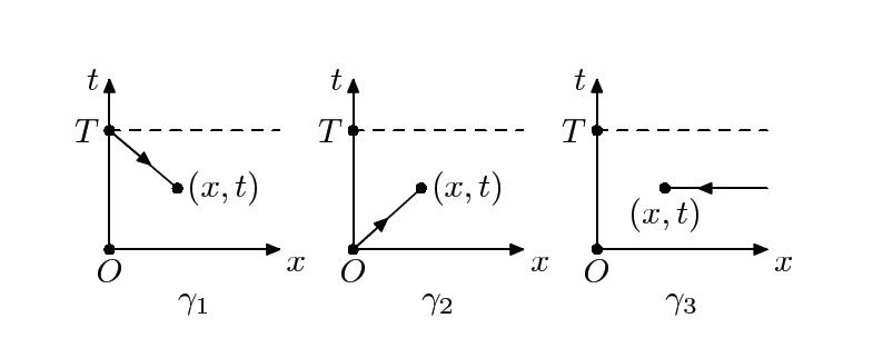
Figure 1: The three contours $\gamma_{1},\gamma_{2},\gamma_{3}$ in the $(x,t)$-domaint

So we have that the following inequalities are hold true on the contours $\gamma_{j}(j=1,2,3)$

$$\begin{array}[]{l}\gamma_{1}=(x_{1},t_{1})\rightarrow(x,t):\,x-\xi\geq 0,\,t-\tau\leq 0,\\ \gamma_{2}=(x_{2},t_{2})\rightarrow(x,t):\,x-\xi\geq 0,\,t-\tau\geq 0,\\ \gamma_{3}=(x_{3},t_{3})\rightarrow(x,t):\,x-\xi\leq 0.\end{array}$$ (2.31)

Define the following sets (see Figure 2) as

$$\begin{array}[]{l}D_{1}=\{\lambda\in C|\mathrm{arg}\lambda\in(0,\frac{\pi}{2})\cup(\pi,\frac{3\pi}{2})$and$|\lambda|>\frac{1}{\sqrt{2}}\},\\ D_{2}=\{\lambda\in C|\mathrm{arg}\lambda\in(0,\frac{\pi}{2})\cup(\pi,\frac{3\pi}{2})$and$|\lambda|<\frac{1}{\sqrt{2}}\},\\ D_{3}=\{\lambda\in C|\mathrm{arg}\lambda\in(\frac{\pi}{2},\pi)\cup(\frac{3\pi}{2},2\pi)$and$|\lambda|<\frac{1}{\sqrt{2}}\},\\ D_{4}=\{\lambda\in C|\mathrm{arg}\lambda\in(\frac{\pi}{2},\pi)\cup(\frac{3\pi}{2},2\pi)$and$|\lambda|>\frac{1}{\sqrt{2}}\}.\end{array}$$ (2.36)

From Eq.(2.4), we have

$$k=\lambda-\frac{1}{2\lambda}=(1-\frac{1}{2|\lambda|^{2}})\mathrm{Re}\lambda+i(1+\frac{1}{2|\lambda|^{2}})\mathrm{Im}\lambda.$$

As the first, second, and third columns of the matrix equation Eq.(2.9) contain the following exponential term

$$\begin{array}[]{l}\mu_{j}^{(1)}:\quad e^{-2i\lambda^{2}(x-\xi)-4ik^{2}t(t-\tau)},\quad e^{-2i\lambda^{2}(x-\xi)-4ik^{2}t(t-\tau)},\\ \mu_{j}^{(2)}:\quad e^{2i\lambda^{2}(x-\xi)+4ik^{2}t(t-\tau)},\\ \mu_{j}^{(3)}:\quad e^{2i\lambda^{2}(x-\xi)+4ik^{2}t(t-\tau)}.\\ \end{array}$$ (2.40)

Thus, these inequalities imply that the function $\mu_{j}(x,t,\lambda)(j=1,2,3)$ is bounded and analytic in the following regions

$$\begin{array}[]{l}\mu_{1}\quad$is bounded for$\quad\lambda\in(D_{4},D_{2},D_{2}),\\ \mu_{2}\quad$is bounded for$\quad\lambda\in(D_{3},D_{1},D_{1}),\\ \mu_{3}\quad$is bounded for$\quad\lambda\in(D_{1}\cup D_{2},D_{3}\cup D_{4},D_{3}\cup D_{4}),\end{array}$$ (2.44)

where $D_{n}(n=1,2,3,4)$ represents a subset of four open disjoint $\lambda-$ plane shown in figure 2.

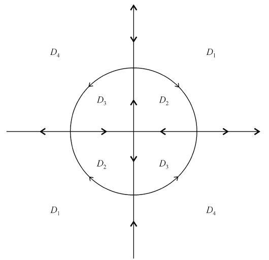
Figure 2: The sets $D_{n},n=1,2,3,4$, which decompose the complex $\lambda-$plane

And these sets $D_{n}(n=1,2,3,4)$ have the following properties

$$\begin{array}[]{l}D_{1}=\{\lambda\in C|\mathrm{Re}l_{1}<\mathrm{Re}l_{2}=\mathrm{Re}l_{3},\quad\mathrm{Re}z_{1}<\mathrm{Re}z_{2}=\mathrm{Re}z_{3}\},\\ D_{2}=\{\lambda\in C|\mathrm{Re}l_{1}<\mathrm{Re}l_{2}=\mathrm{Re}l_{3},\quad\mathrm{Re}z_{1}>\mathrm{Re}z_{2}=\mathrm{Re}z_{3}\},\\ D_{3}=\{\lambda\in C|\mathrm{Re}l_{1}>\mathrm{Re}l_{2}=\mathrm{Re}l_{3},\quad\mathrm{Re}z_{1}<\mathrm{Re}z_{2}=\mathrm{Re}z_{3}\},\\ D_{4}=\{\lambda\in C|\mathrm{Re}l_{1}>\mathrm{Re}l_{2}=\mathrm{Re}l_{3},\quad\mathrm{Re}z_{1}>\mathrm{Re}z_{2}=\mathrm{Re}z_{3}\},\end{array}$$ (2.49)

where $l_{i}(\lambda)$ and $z_{i}(\lambda)$ are the diagonal elements of the matrix $-i\lambda^{2}\sigma$ and $-2ik^{2}\sigma$.

In fact, $\mu_{1}(0,t,\lambda)$ has a larger bounded and analytic domain $(D_{1}\cup D_{4},D_{2}\cup D_{3},D_{2}\cup D_{3})$ for $x=0$, and it is not difficult to see that $\mu_{2}(0,t,\lambda)$ has also a larger bounded and analytic domain $(D_{2}\cup D_{3},D_{1}\cup D_{4},D_{1}\cup D_{4})$ for $x=0$.

2.3 The matrix value eigenfunction

For each $n=1,2,3,4$, a solution $M_{n}(x,t,\lambda)$ of Eq.(2.6) is defined by the following integral equation

$$(M_{n}(x,t,\lambda))_{ij}=\delta_{ij}+\int_{\gamma_{ij}^{n}}(e^{(i\lambda^{2}x+2ik^{2}t)\hat{\sigma}}W_{n}(\xi,\tau,\lambda))_{ij},\quad i,j=1,2,3,$$ (2.50)

where $W_{n}(x,t,\lambda)$ is given by Eq.(2.8), it is only used $M_{n}$ in place of $\mu$, and the contours $\gamma_{ij}^{n}(n=1,2,3,4;i,j=1,2,3)$ are defined as follows

$$\gamma_{ij}^{n}=\left\{\begin{array}[]{l}\gamma_{1}\quad if\quad\mathrm{Re}l_{i}(\lambda)<\mathrm{Re}l_{j}(\lambda)\quad and\quad\mathrm{Re}z_{i}(\lambda)\geq\mathrm{Re}z_{j}(\lambda)\\ \gamma_{2}\quad if\quad\mathrm{Re}l_{i}(\lambda)<\mathrm{Re}l_{j}(\lambda)\quad and\quad\mathrm{Re}z_{i}(\lambda)<\mathrm{Re}z_{j}(\lambda)\\ \gamma_{3}\quad if\quad\mathrm{Re}l_{i}(\lambda)\geq\mathrm{Re}l_{j}(\lambda)\\ \end{array}\right.for\lambda\in D_{n}\quad$$ (2.54)

According to the definition of $\gamma^{n}$, we have

$$\begin{array}[]{l}\gamma^{1}=\left(\begin{array}[]{ccc}\gamma_{3}&\gamma_{2}&\gamma_{2}\\ \gamma_{3}&\gamma_{3}&\gamma_{3}\\ \gamma_{3}&\gamma_{3}&\gamma_{3}\end{array}\right),\,\gamma^{2}=\left(\begin{array}[]{ccc}\gamma_{3}&\gamma_{1}&\gamma_{1}\\ \gamma_{3}&\gamma_{3}&\gamma_{3}\\ \gamma_{3}&\gamma_{3}&\gamma_{3}\end{array}\right),\\ \gamma^{3}=\left(\begin{array}[]{ccc}\gamma_{3}&\gamma_{3}&\gamma_{3}\\ \gamma_{1}&\gamma_{3}&\gamma_{3}\\ \gamma_{1}&\gamma_{3}&\gamma_{3}\end{array}\right),\,\gamma^{4}=\left(\begin{array}[]{ccc}\gamma_{3}&\gamma_{3}&\gamma_{3}\\ \gamma_{2}&\gamma_{3}&\gamma_{3}\\ \gamma_{2}&\gamma_{3}&\gamma_{3}\end{array}\right).\end{array}$$ (2.69)

Next, the following proposition guarantees that the previous definition of $M_{n}$ has properties that can be represented as a Rimann-Hilbert problem.

Proposition 2.1

For each $n=1,2,3,4$ and $\lambda\in D_{n}$, the function $M_{n}(x,t,\lambda)$ is defined well by Eq.(2.14). For any identified point $(x,t)$, $M_{n}$ is bounded and analytic as a function of $\lambda\in D_{n}$ away from a possible discrete set of singularities $\{\lambda_{j}\}$ at which the Fredholm determinant vanishes. Moreover, $M_{n}$ admits a bounded and continuous extension to $\bar{D}_{n}$ and

$$M_{n}(x,t,\lambda)=\mathbb{I}+O(\frac{1}{\lambda}).$$ (2.70)

Proof: The associated bounded and analytic properties have been established in Appendix B in [24]. Substituting the follow expansion

$$M=M_{0}+\frac{M^{(1)}}{\lambda}+\frac{M^{(2)}}{\lambda^{2}}+\frac{M^{(3)}}{\lambda^{3}}+\frac{M^{(4)}}{\lambda^{4}}+\cdots,\quad\lambda\rightarrow\infty,$$

into the Lax pair Eq.(2.6) and comparing the coefficients of $\lambda$ can obtain (2.7).

2.4 The jump matrix

Define the spectral function as follows

$$S_{n}(\lambda)=M_{n}(0,0,\lambda),\quad\lambda\in D_{n},n=1,2,3,4.$$ (2.71)

Let $M$ be a sectionally analytical continuous function in Riemann $\lambda-$ sphere which equals $M_{n}$ for $\lambda\in D_{n}$. So, $M$ satisfies the following jump conditions

$$M_{n}(\lambda)=M_{m}J_{m,n},\quad\lambda\in\bar{D}_{n}\cap\bar{D}_{m},\quad n,m=1,2,3,4;n\neq m,$$ (2.72)

where

$$J_{m,n}=e^{(-ikx+2ik^{2}t)\hat{\Lambda}}(S_{m}^{-1}S_{n}).$$ (2.73)

2.5 The adjugated eigenfunction

Likewise, we also need to consider the bounded and analytic properties of the minors of the matrices $\mu_{j}(x,t,\lambda)(j=1,2,3)$. We recall that the cofactor matrix $B^{A}$ of a $3\times 3$ matrix $B$ is defined by

$$B^{A}=\left(\begin{array}[]{ccc}m_{11}(B)&-m_{12}(B)&m_{13}(B)\\ -m_{21}(B)&m_{22}(B)&-m_{23}(B)\\ m_{31}(B)&-m_{32}(B)&m_{33}(B)\end{array}\right),$$

where $m_{ij}(B)$ denote the $(ij)$th minor of $B$. From Eq.(2.6) we find that the adjugated eigenfunction $\mu^{A}$ satisfies the Lax pair

$$\left\{\begin{array}[]{l}\mu_{x}^{A}+i\lambda^{2}[\sigma,\mu^{A}]=-V_{1}^{T}\mu^{A},\\ \mu_{t}^{A}+2ik^{2}[\sigma,\mu^{A}]=-V_{2}^{T}\mu^{A},\end{array}\right.$$ (2.76)

where $V^{T}$ denotes the transform of a matrix $V$. So, the adjugated eigenfunctions $\mu_{j}(j=1,2,3)$ are solutions of the integral equations

$$\mu_{j}^{A}(x,t,\lambda)=I-\int_{\gamma_{j}}e^{(-i\lambda^{2}(x-\xi)-2ik^{2}(t-\tau))\hat{\sigma}}(V_{1}^{T}dx+V_{2}^{T}dt),\quad j=1,2,3,$$ (2.77)

Thus, we can obtain the adjugated eigenfunction which satisfies the following analytic properties

$$\begin{array}[]{l}\mu_{1}^{A}\quad$is bounded for$\quad\lambda\in(D_{2},D_{4},D_{4}),\\ \mu_{2}^{A}\quad$is bounded for$\quad\lambda\in(D_{1},D_{3},D_{3}),\\ \mu_{3}^{A}\quad$is bounded for$\quad\lambda\in(D_{3}\cup D_{4},D_{1}\cup D_{2},D_{1}\cup D_{2}).\end{array}$$ (2.81)

In fact, $\mu_{1}^{A}(0,t,\lambda)$ has a larger bounded and analytic domain which is $(D_{2}\cup D_{3},D_{1}\cup D_{4},D_{1}\cup D_{4})$ for $x=0$, and $\mu_{2}^{A}(0,t,\lambda)$ also has a larger bounded analytic domain which is $(D_{1}\cup D_{4},D_{2}\cup D_{3},D_{2}\cup D_{3})$ for $x=0$.

2.6 Symmetry

By the following Lemma, we show that the eigenfunctions $\mu_{j}(x,t,\lambda)$ have an important symmetry.

Lemma 2.2

The eigenfunction $\psi(x,t,\lambda)$ of the Lax pair Eq.(2.1) admits the following symmetry

$$\psi^{-1}(x,t,\lambda)=A\overline{\psi(x,t,\bar{\lambda})}^{T}A,$$

with

$$A=\left(\begin{array}[]{ccc}-1&0&0\\ 0&\varepsilon&0\\ 0&0&\varepsilon\end{array}\right),\quad and\quad\varepsilon^{2}=1.$$

where the superscript T denotes a matrix transpose.

Proof: Analogous to the proof provided in [24]. We omit the proof.

Remark 2.3

From Lemma 1, one can show that the eigenfunctions $\mu_{j}(x,t,\lambda)$ of Lax pair Eq.(2.6) have the same symmetry.

2.7 The jump matrix computation

We define $3\times 3$ matrix value function $s(\lambda)$ and $S(\lambda)$ as follows

$$\begin{array}[]{l}\mu_{3}(x,t,\lambda)=\mu_{2}(x,t,\lambda)e^{(i\lambda^{2}x+2ik^{2}t)\hat{\sigma}}s(\lambda),\\ \mu_{1}(x,t,\lambda)=\mu_{2}(x,t,\lambda)e^{(i\lambda^{2}x+2ik^{2}t)\hat{\sigma}}S(\lambda),\end{array}$$ (2.84)

as $\mu_{2}(0,0,\lambda)=\mathbb{I}$, we obtain

$$s(\lambda)=\mu_{3}(0,0,\lambda),\quad S(\lambda)=\mu_{1}(0,0,\lambda).$$ (2.85)

From the properties of $\mu_{j}$ and $\mu_{j}^{A}(j=1,2,3)$ we can obtain that $s(\lambda)$ and $S(\lambda)$ have the following bounded and analytic properties

$$\begin{array}[]{l}s(\lambda)\quad$is bounded for$\quad\lambda\in(D_{1}\cup D_{2},D_{3}\cup D_{4},D_{3}\cup D_{4}),\\ S(\lambda)\quad$is bounded for$\quad\lambda\in(D_{1}\cup D_{4},D_{2}\cup D_{3},D_{2}\cup D_{3}),\\ s^{A}(\lambda)\quad$is bounded for$\quad\lambda\in(D_{3}\cup D_{4},D_{1}\cup D_{2},D_{1}\cup D_{2}),\\ S^{A}(\lambda)\quad$is bounded for$\quad\lambda\in(D_{2}\cup D_{3},D_{1}\cup D_{4},D_{1}\cup D_{4}),\end{array}$$ (2.90)

moreover

$$M_{n}(x,t,\lambda)=\mu_{2}(x,t,\lambda)e^{(i\lambda^{2}x+2ik^{2}t)\hat{\sigma}}S_{n}(\lambda),\quad\lambda\in D_{n}.$$ (2.91)

Proposition 2.4

$S_{n}$ can be expressed with $s(\lambda)$ and $S(\lambda)$ elements as follows

$$\begin{array}[]{l}S_{1}=\left(\begin{array}[]{ccc}s_{11}&0&0\\ s_{21}&\frac{m_{33}(s)}{s_{11}}&\frac{m_{32}(s)}{s_{11}}\\ s_{31}&\frac{m_{23}(s)}{s_{11}}&\frac{m_{22}(s)}{s_{11}}\end{array}\right),\\ S_{2}=\left(\begin{array}[]{ccc}s_{11}&\frac{m_{33}(s)M_{21}(S)-m_{23}(s)M_{31}(S)}{(s^{T}S^{A})_{11}}&\frac{m_{32}(s)M_{21}(S)-m_{22}(s)M_{31}(S)}{(s^{T}S^{A})_{11}}\\ s_{21}&\frac{m_{33}(s)M_{11}(S)-m_{13}(s)M_{31}(S)}{(s^{T}S^{A})_{11}}&\frac{m_{32}(s)M_{11}(S)-m_{12}(s)M_{31}(S)}{(s^{T}S^{A})_{11}}\\ s_{31}&\frac{m_{23}(s)M_{11}(S)-m_{13}(s)M_{21}(S)}{(s^{T}S^{A})_{11}}&\frac{m_{22}(s)M_{11}(S)-m_{12}(s)M_{21}(S)}{(s^{T}S^{A})_{11}}\end{array}\right),\\ S_{3}=\left(\begin{array}[]{ccc}\frac{S_{11}}{(S^{T}s^{A})_{11}}&s_{12}&s_{13}\\ \frac{S_{21}}{(S^{T}s^{A})_{11}}&s_{22}&s_{23}\\ \frac{S_{31}}{(S^{T}s^{A})_{11}}&s_{32}&s_{33}\end{array}\right),S_{4}=\left(\begin{array}[]{ccc}\frac{1}{m_{11}(s)}&s_{12}&s_{13}\\ 0&s_{22}&s_{23}\\ 0&s_{32}&s_{33}\end{array}\right),\end{array}$$ (2.107)

where $(S^{T}s^{A})_{11}$ and $(s^{T}S^{A})_{11}$ are defined as follows

$$\begin{array}[]{l}(S^{T}s^{A})_{11}=S_{11}m_{11}(s)-S_{21}m_{21}(s)+S_{31}m_{31}(s),\\ (s^{T}S^{A})_{11}=s_{11}m_{11}(S)-s_{21}m_{21}(S)+s_{31}m_{31}(S).\end{array}$$ (2.110)

Proof: We set $\gamma_{3}^{X_{0}}$ is a contour when $(X_{0},0)\rightarrow(x,t)$ in the $(x,t)$-plane, here $X_{0}$ is a constant and $X_{0}>0$, for $j=3$, we introduce $\mu_{3}(x,t,\lambda;X_{0})$ as the solution of Eq.(2.9) with the contour $\gamma_{3}$ replaced by $\gamma_{3}^{X_{0}}$. Similarly, we define $M_{n}(x,t,\lambda;X_{0})$ as the solution of Eq.(2.14) with $\gamma_{3}$ replaced by $\gamma_{3}^{X_{0}}$. Then, by simple calculation, we can derive the expression of $S_{n}(\lambda,X_{0})=M_{n}(0,0,\lambda;X_{0})$ with $S(\lambda)$ and $s(\lambda;X_{0})$ and the Eq.(2.28) will be obtain by taking the limit $X_{0}\rightarrow\infty$.

Firstly, we have the following relations:

$$M_{n}(x,t,\lambda;X_{0})=\mu_{1}(x,t,\lambda)e^{(i\lambda^{2}x+2ik^{2}t)\hat{\sigma}}R_{n}(\lambda;X_{0}),$$ (2.111)

$$M_{n}(x,t,\lambda;X_{0})=\mu_{2}(x,t,\lambda)e^{(i\lambda^{2}x+2ik^{2}t)\hat{\sigma}}S_{n}(\lambda;X_{0}),$$ (2.112)

$$M_{n}(x,t,\lambda;X_{0})=\mu_{3}(x,t,\lambda)e^{(i\lambda^{2}x+2ik^{2}t)\hat{\sigma}}T_{n}(\lambda;X_{0}).$$ (2.113)

Secondly, we get the definition of $R_{n}(\lambda;X_{0})$ and $T_{n}(\lambda;X_{0})$ as follows

$$R_{n}(\lambda;X_{0})=e^{-2ik^{2}T\hat{\sigma}}M_{n}(0,T,\lambda;X_{0}),$$ (2.114)

$$T_{n}(\lambda;X_{0})=e^{-i\lambda^{2}X_{0}\hat{\sigma}}M_{n}(X_{0},0,\lambda;X_{0}),$$ (2.115)

the Eq.(2.30) means that

$$s(\lambda;X_{0})=S_{n}(\lambda;X_{0})T_{n}^{-1}(\lambda;X_{0}),$$ (2.116)

$$S(\lambda;X_{0})=S_{n}(\lambda;X_{0})R_{n}^{-1}(\lambda;X_{0}).$$ (2.117)

These equations constitute the matrix decomposition problem of $\{s,S\}$ by use $\{R_{n},S_{n},T_{n}\}$. In fact, by the definition of the integral equation Eq.(2.14) and $\{R_{n},S_{n},T_{n}\}$, we obtain

$$\left\{\begin{array}[]{l}(R_{n}(\lambda;X_{0}))_{ij}=0\quad if\quad\gamma_{ij}^{n}=\gamma_{1},\\ (S_{n}(\lambda;X_{0}))_{ij}=0\quad if\quad\gamma_{ij}^{n}=\gamma_{2},\\ (S_{n}(\lambda;X_{0}))_{ij}=\delta_{ij}\quad if\quad\gamma_{ij}^{n}=\gamma_{3}.\end{array}\right.$$ (2.121)

Thus Eq.(2.31) are the eighteen scalar equations with eighteen unknowns. The exact solution of these system can be obtained by solving the algebraic system. In this way, we can get a similar $\{S_{n}(\lambda),s(\lambda)\}$ as in Eq.(2.28) which just that $\{S_{n}(\lambda),s(\lambda)\}$ replaces by $\{S_{n}(\lambda;X_{0}),s(\lambda;X_{0})\}$ in Eq.(2.28).

Finally, taking $X_{0}\rightarrow\infty$ in this equation, we obtain the Eq.(2.28).

2.8 The residue conditions

As $\mu_{2}$ is an entire function and by Eq.(2.27), it is not difficult to see that $M$ only produces singularities in $S_{n}$ where there are singular points, from the exact expression Eq.(2.28), we found that $M$ may be singular as follows

(1)$[M_{1}]_{2}$ and $[M_{1}]_{3}$ could have poles in $D_{1}$ at the zeros of $s_{11}(\lambda)$,

(2)$[M_{2}]_{2}$ and $[M_{2}]_{3}$ could have poles in $D_{2}$ at the zeros of $(s^{T}S^{A})_{11}(\lambda)$,

(3)$[M_{3}]_{1}$ could have poles in $D_{3}$ at the zeros of $(S^{T}s^{A})_{11}(\lambda)$,

(4)$[M_{4}]_{1}$ could have poles in $D_{4}$ at the zeros of $m_{11}(s)(\lambda)$.

We use $\lambda_{j}(j=1,2\cdots N)$ denote the possible zero point of $M$ in $D_{n}$, and assume that these possible zeros satisfy the following assumptions.

Assumption 2.5

Assume that

(1)$s_{11}(\lambda)$ has $n_{0}$ possible simple zeros in $D_{1}$ denoted by $\lambda_{j},j=1,2\cdots n_{0}$,

(2)$(s^{T}S^{A})_{11}(\lambda)$ has $n_{1}-n_{0}$ possible simple zeros in $D_{2}$ denoted by $\lambda_{j},j=n_{0}+1,n_{0}+2\cdots n_{1}$,

(3)$(S^{T}s^{A})_{11}(\lambda)$ has $n_{2}-n_{1}$ possible simple zeros in $D_{3}$ denoted by $\lambda_{j},j=n_{1}+1,n_{1}+2\cdots n_{2}$,

(4)$m_{11}(s)(\lambda)$ has $N-n_{2}$ possible simple zeros in $D_{4}$ denoted by $\lambda_{j},j=n_{2}+2,n_{2}+2\cdots N$,

And these zeros are different, moreover assuming that there is no zero on the boundary of $D_{n}(n=1,2,3,4)$.

Proposition 2.6

Let $M_{n}(n=1,2,3,4)$ be the eigenfunctions defined by (2.14) and assume that the set $\lambda_{j}(j=1,2\cdots N)$ of singularities are as the above assumption. Then the following residue conditions hold true:

$$\mathrm{Re}s_{\lambda=\lambda_{j}}[M]_{2}=\frac{m_{33}(s)(\lambda_{j})}{\dot{s_{11}(\lambda_{j})}s_{21}(\lambda_{j})}e^{\theta_{13}(\lambda_{j})}[M(\lambda_{j})]_{1},\quad 1\leq j\leq n_{0};\lambda_{j}\in D_{1}.$$ (2.122)

$$\mathrm{Re}s_{\lambda=\lambda_{j}}[M]_{3}=\frac{m_{32}(s)(\lambda_{j})}{\dot{s_{11}(\lambda_{j})}s_{21}(\lambda_{j})}e^{\theta_{13}(\lambda_{j})}[M(\lambda_{j})]_{1},\quad 1\leq j\leq n_{0};\lambda_{j}\in D_{1}.$$ (2.123)

$$\mathrm{Re}s_{\lambda=\lambda_{j}}[M]_{2}=\frac{m_{33}(s)(\lambda_{j})M_{11}(S)(\lambda_{j})-m_{13}(s)(\lambda_{j})M_{31}(S)(\lambda_{j})}{\dot{(s^{T}S^{A})_{11}(\lambda_{j})}s_{21}(\lambda_{j})}e^{\theta_{13}(\lambda_{j})}[M(\lambda_{j})]_{1},$$

$$\qquad\qquad\qquad n_{0}+1\leq j\leq n_{1};\lambda_{j}\in D_{2}.$$ (2.124)

$$\mathrm{Re}s_{\lambda=\lambda_{j}}[M]_{3}=\frac{m_{32}(s)(\lambda_{j})M_{11}(S)(\lambda_{j})-m_{12}(s)(\lambda_{j})M_{31}(S)(\lambda_{j})}{\dot{(s^{T}S^{A})_{11}(\lambda_{j})}s_{21}(\lambda_{j})}e^{\theta_{13}(\lambda_{j})}[M(\lambda_{j})]_{1},$$

$$\qquad\qquad\qquad n_{0}+1\leq j\leq n_{1};\lambda_{j}\in D_{2}.$$ (2.125)

$$\mathrm{Re}s_{\lambda=\lambda_{j}}[M]_{1}=\frac{s_{33}(\lambda_{j})S_{21}(\lambda_{j})-s_{23}(\lambda_{j})S_{31}(\lambda_{j})}{\dot{(S^{T}s^{A})_{11}(\lambda_{j})}m_{11}(s)(\lambda_{j})}e^{\theta_{31}(\lambda_{j})}[M(\lambda_{j})]_{2}$$

$$\qquad\quad+\frac{s_{22}(\lambda_{j})S_{31}(\lambda_{j})-s_{32}(\lambda_{j})S_{21}(\lambda_{j})}{\dot{(S^{T}s^{A})_{11}(\lambda_{j})}m_{11}(s)(\lambda_{j})}e^{\theta_{31}(\lambda_{j})}[M(\lambda_{j})]_{3},n_{1}+1\leq j\leq n_{2};\lambda_{j}\in D_{3}.$$ (2.126)

$$\mathrm{Re}s_{\lambda=\lambda_{j}}[M]_{1}=\frac{s_{33}(\lambda_{j})[M_{(}\lambda_{j})]_{2}-s_{32}(\lambda_{j})[M_{(}\lambda_{j})]_{3}}{\dot{m_{11}(s)(\lambda_{j})}m_{21}(s)(\lambda_{j})}e^{\theta_{31}(\lambda_{j})},n_{2}+1\leq j\leq N;\lambda_{j}\in D_{4}.$$ (2.127)

where $\dot{f}=\frac{df}{d\lambda}$ and $\theta_{ij}$ given by

$$\theta_{ij}(x,t,\lambda)=(l_{i}-l_{j})x-(z_{i}-z_{j})t\quad i,j=1,2,3,$$ (2.128)

thus

$$\theta_{ij}=0,\quad i,j=2,3,\quad\theta_{12}=\theta_{13}=-\theta_{21}=-\theta_{31}=2i\lambda^{2}x-4ik^{2}t.$$

Proof: We will only prove (2.39), (2.40) and the other conditions follow by similar arguments. The equation (2.27) means that

$$M_{2}=\mu_{2}e^{(i\lambda^{2}x+2ik^{2}t)\hat{\sigma}}S_{2},$$ (2.129)

In view of the expression for $S_{2}$ given in (2.28), the three columns of Eq.(2.44) read

$$[M_{2}]_{1}=[\mu_{2}]_{1}s_{11}+[\mu_{2}]_{2}s_{21}e^{\theta_{31}}+[\mu_{2}]_{3}s_{31}e^{\theta_{31}},$$ (2.130)

$$[M_{2}]_{2}=\frac{m_{33}(s)M_{21}(S)-m_{23}(s)M_{31}(S)}{(s^{T}S^{A})_{11}}e^{\theta_{13}}[\mu_{2}]_{1}+\frac{m_{33}(s)M_{11}(S)-m_{13}(s)M_{31}(S)}{(s^{T}S^{A})_{11}}[\mu_{2}]_{2}$$

$$\qquad\quad+\frac{m_{23}(s)M_{11}(S)-m_{13}(s)M_{21}(S)}{(s^{T}S^{A})_{11}}[\mu_{2}]_{3},$$ (2.131)

$$[M_{2}]_{3}=\frac{m_{32}(s)M_{21}(S)-m_{22}(s)M_{31}(S)}{(s^{T}S^{A})_{11}}e^{\theta_{13}}[\mu_{2}]_{1}+\frac{m_{32}(s)M_{11}(S)-m_{12}(s)M_{31}(S)}{(s^{T}S^{A})_{11}}[\mu_{2}]_{2}$$

$$\qquad\quad+\frac{m_{22}(s)M_{11}(S)-m_{12}(s)M_{21}(S)}{(s^{T}S^{A})_{11}}[\mu_{2}]_{3}.$$ (2.132)

Let $\lambda_{j}\in D_{2}$ be a simple zero of $(s^{T}S^{A})_{11}(\lambda)$. Solving Eq.(2.45) for $[\mu_{2}]_{2}$ and substituting the result into Eq.(2.46) and Eq.(2.47) yields

$$[M_{2}]_{2}=\frac{m_{33}(s)M_{11}(S)-m_{13}(s)M_{31}(S)}{(s^{T}S^{A})_{11}s_{21}}e^{\theta_{13}}[M_{1}]_{1}-\frac{m_{33}(s)}{s_{21}}e^{\theta_{13}}[\mu_{2}]_{1}+\frac{m_{13}(s)}{s_{21}}[\mu_{2}]_{3},$$ (2.133)

$$[M_{2}]_{3}=\frac{m_{32}(s)M_{11}(S)-m_{12}(s)M_{31}(S)}{(s^{T}S^{A})_{11}s_{21}}e^{\theta_{13}}[M_{1}]_{1}-\frac{m_{32}(s)}{s_{21}}e^{\theta_{13}}[\mu_{2}]_{1}+\frac{m_{12}(s)}{s_{21}}[\mu_{2}]_{3}.$$ (2.134)

Taking the residue of the two equations at $\lambda_{j}$, we find conditions Eq.(2.39) and Eq.(2.40) in the case when $\lambda_{j}\in D_{2}$.

2.9 The global relation

The spectral functions $S(\lambda)$ and $s(\lambda)$ are not independent which is of important relationship each other. In fact, from Eq.(2.24), we not difficult to find that

$$\mu_{3}(x,t,\lambda)=\mu_{1}(x,t,\lambda)e^{(i\lambda^{2}x+2ik^{2}t)\hat{\sigma}}S^{-1}(\lambda)s(\lambda),\lambda\in(D_{1}\cup D_{2},D_{3}\cup D_{4},D_{3}\cup D_{4}),$$ (2.135)

as $\mu_{1}(0,t,\lambda)=\mathbb{I}$, when $(x,t)=(0,T)$, We can evaluate the following relationship which is the global relation

$$S^{-1}(\lambda)s(\lambda)=e^{-2ik^{2}T\hat{\sigma}}c(T,\lambda),\quad\lambda\in(D_{1}\cup D_{2},D_{3}\cup D_{4},D_{3}\cup D_{4}),$$ (2.136)

where $c(T,\lambda)=\mu_{3}(0,t,\lambda)$.

3 The Riemann-Hilbert problem

In section 2, we defined the sectionally analytical function $M(x,t,\lambda)$ that its satisfies a Riemann-Hilbert problem which can be formulated in terms of the initial values and boundary values of $\{q(x,t),r(x,t)\}$. For all $(x,t)$, the $\{q_{x}(x,t),r_{x}(x,t)\}$ can be recovered by solving this Riemann-Hilbert problem, and the solution $\{q(x,t),r(x,t)\}$ of Eq.(1.4) can be obtained by integration with respect to $x$. So we have the following theorem is established.

Theorem 3.1

Suppose that the half-line domain $\Omega=\{0<x<\infty,0<t<T\}$ with sufficient smoothness and decays as $x\rightarrow\infty$, and assume that $\{q(x,t),r(x,t)\}$ is a solution of Eq.(1.4) in half-line domain $\Omega$ which can be reconstructed from the initial value $\{q_{0}(x),r_{0}(x)\}$ and boundary values $\{g_{0}(t),h_{0}(t),g_{1}(t),h_{1}(t)\}$ lie in the Schwartz class defined as follows.

$$\begin{array}[]{l}q_{0}(x)=u(x,t=0),\;r_{0}(x)=v(x,t=0),\\ g_{0}(t)=q(x=0,t),\;h_{0}(t)=r(x=0,t),\\ g_{1}(t)=q_{x}(x=0,t),\;h_{1}(t)=r_{x}(x=0,t),\end{array}$$ (3.4)

like Eq.(2.24) using the initial data and boundary data to define the spectral functions $s(\lambda)$ and $S(\lambda)$,further defining the jump matrix $J_{m,n}(x,t,\lambda)$. Assume that the zero point of the $s_{11}(\lambda),(s^{T}S^{A})_{11}(\lambda),(S^{T}s^{A})_{11}(\lambda)$ and $m_{11}(s)(\lambda)$ is $\lambda_{j}(j=1,2\cdots N)$ are as in assumption 2.5, that is the following assumptions.

Then the $\{q_{x}(x,t),r_{x}(x,t)\}$ of Eq.(1.4) is

$$\begin{array}[]{l}q_{x}(x,t)=-2i\lim_{\lambda\rightarrow\infty}(\lambda M(x,t,\lambda))_{12},\\ r_{x}(x,t)=-2i\lim_{\lambda\rightarrow\infty}(\lambda M(x,t,\lambda))_{13},\end{array}$$ (3.7)

where $M(x,t,\lambda)$ satisfies the following $3\times 3$ matrix Riemann-Hilbert problem:

(1)$M$ is a sectionally meromorphic on the Riemann $\lambda$-sphere with jumps across the contours on $\bar{D}_{n}\cap\bar{D}_{m}(n,m=1,2,3,4)$ (see figure 2).

(2)$M$ satisfies the jump condition with jumps across the contours on $\bar{D}_{n}\cap\bar{D}_{m}(n,m=1,2,3,4)$

$$M_{n}(\lambda)=M_{m}J_{m,n},\quad\lambda\in\bar{D}_{n}\cap\bar{D}_{m},n,m=1,2,3,4;n\neq m.$$ (3.8)

(3)$M(x,t,\lambda)=\mathbb{I}+O(\frac{1}{\lambda}),\quad\lambda\rightarrow\infty.$

(4)The residue condition of $M$ is showed in Proposition 2.6.

Proof: We can use similar method with[33] to prove this Theorem. It only need to prove Eq.(3.2) and this equation follows from the large $\lambda$ asymptotics of the eigenfunctions.

Thus, the solution of the coupled Fokas-Lenells equations $\{q(x,t),r(x,t)\}$ can be obtained by integration with respect to $x$.

4 Conclusions and discussions

In this paper, we consider IBV of the CFL equation on the half-line. Using the unified transform method for nonlinear evolution systems which taking the form of Lax pair isospectral deformations and whose corresponding continuous spectra Lax operators, assume that the solutions $q(x,t)$ and $r(x,t)$ exists, we show that it can be represented in terms of the solution of a matrix Riemann-Hilbert problem formulated in the plane of the complex spectral parameter $\lambda$. For other $3\times 3$ matrix Lax pair integrable equations, can we construct their solution of a matrix Riemann-Hilbert problem formulated in the plane of the complex spectral parameter $\lambda$ by the similar method? In paper [32], Xu and Fan use the Deift-Zhou method to studied the long-time asymptotics for the solutions of the decay initial value on the full-line. Moreover, under the assumption that the initial and boundary values lie in the Schwartz class, Chen and Yan have successfully applied the nonlinear steepest descent method to analyze the long-time asymptotic for the solution of decay IBV problem of the FL equation on the half line in [6], can we do the long-time asymptotics for the solutions of the decay initial and boundary values of CFL equations following the same ways as for the DP equation [5]? These questions will be discussed in our future work.

Acknowledgements

This work is partially supported by the National Natural Science Foundation of China under Grant Nos. 12271008 and 11601055, Natural Science Foundation of Anhui Province under Grant No.1408085QA06.

References

- [1] Boutet de Monvel A, and Shepelsky D, A Riemann-Hilbert approach for the Degasperis-Procesi equation, Nonlinearity 26 (2013), 2081-2107.
- [2] Boutet de Monvel A, and Shepelsky D, The Ostrovsky-Vakhnenko equation: A Riemann-Hilbert approach, C. R. Acad. Sci. Paris, Ser. I 352(2014), 189-195.
- [3] Boutet de Monvel A, and Shepelsky D, The Ostrovsky-Vakhnenko equation by a Riemann-Hilbert approach, J. Phys. A: Math. Theor. 48 (2015), 035204.
- [4] Boutet de Monvel A, Shepelsky D, and Zielinski L, A Riemann-Hilbert approach for the Novikov equation, SIGMA 12 2016, 095.
- [5] Boutet de Monvel A, Lenells J, and Shepelsky D, Long-time asymptotics for the Degasperis-Procesi equation on the half-line, 2015, arxiv: 1508.04097.
- [6] Chen S Y, Yan Z Y. Long-time asymptotics for initial-boundary value problems of integrable Fokas-Lenells equation on the half-line, 2017, arxiv: 1710.06563.
- [7] Deconinck B, Guo Q, Shlizerman E, and Vasan V, Fokas’s Unified Transform Method for linear systems, 2017, arxiv: 1705.00358.
- [8] Deift P, and Zhou X, A steepest descent method for oscillatory Riemann-Hilbert problems, Ann. Math. 137 (1993), 295-368.
- [9] Fokas A S, On a class of physically important integrable equations, Physica. D 87 (1995), 145-150.
- [10] Fokas A S, A unified transform method for solving linear and certain nonlinear PDEs, Proc. R. Soc. Lond. A 453 (1997), 1411-1443.
- [11] Fokas A S, Integrable nonlinear evolution equations on the half-line, Commun. Math. Phys. 230 (2002), 1-39.
- [12] Fokas A S, Its A R, and Sung L Y, The nonlinear Schrödinger equation on the half-line, Nonlinearity 18 (2005), 1771-1822.
- [13] Fokas A S, A unified approach to boundary value problems. CBMS-NSF Regional Conference Series in Applied Mathematics. Philadelphia, PA: Society of Industrial and Applied Mathematics, 2008
- [14] Geng X G, Liu H, and Zhu J Y, Initial-boundary value problems for the coupled nonlinear Schrödinger equation on the half-line, Stud. Appl. Math. 135 (2015), 310-346.
- [15] He J S, Xu S W, and Porsezian K, Rogue Waves of the Fokas-Lenells Equation, J. Phys. Soc. Japan 81 (2012), 124007.
- [16] Hu B B, Xia T C, and Zhang N, A Riemann-Hilbert Approach to the Kundu-Eckhaus Equation on the half-Line, 2017, arxiv: 1711.02516.
- [17] Hu B B, and Xia T C, The coupled modified nonlinear Schrödinger equations on the half-line via the Fokas method, 2017, arxiv: 1704.03623.
- [18] Hu B B, Xia T C, Zhang L, and Wang J B, Initial-boundary value problems for the coupled higher-order nonlinear Schrödinger equations on the half-line. Accepted by International Journal of Nonlinear Sciences and Numerical Simulation.
- [19] Lenells J, Exactly Solvable Model for Nonlinear Pulse Propagation in Optical Fibers, Stud. Appl. Math. 123 (2009), 215-232.
- [20] Lenells J, and Fokas A S, On a novel integrable generalization of the nonlinear Schrödinger equation, Nonlinearity 22 (2009),11-27.
- [21] Lenells J, Dressing for a Novel Integrable Generalization of the Nonlinear Schrödinger Equation, J. Nonlinear Sci. 20 (2010), 709-722.
- [22] Lenells J, and Fokas A S, Boundary-value problems for the stationary axisymmetric Einstein equations: a rotating disc, Nonlinearity 24 (2011), 177-206.
- [23] Lenells J, Boundary value problems for the stationary axisymmetric Einstein equations: a disk rotating around a black hole, Comm. Math. Phys. 304 (2011), 585-635.
- [24] Lenells J, Initial-boundary value problems for integrable evolution equations with Lax pairs, Phys. D 241 (2012), 857-875.
- [25] Lenells J, The Degasperis-Procesi equation on the half-line, Nonlinear Anal. 76 (2013), 122-139.
- [26] Lü X, and Peng M S, Nonautonomous motion study on accelerated and decelerated solitons for the variable-coefficient Lenells-Fokas model, Chaos 23 (2013), 013122.
- [27] Liu H, and Geng X G, Initial-boundary problems for the vector modified Korteweg-deVries equation via Fokas unified transform method, J. Math. Anal. Appl. 440 (2016), 578-596.
- [28] Ling L M, Feng B F, and Zhu Z N, General soliton solutions to a coupled Fokas-Lenells equation, Nonlinear Analysis: Real World Applications 40 (2018), 185-214.
- [29] Matsuno Y, A direct method of solution for the Fokas-Lenells derivative nonlinear Schrödinger equation: II. Dark soliton solutions, J. Phys. A 45 (2012), 475202.
- [30] Tian S F, Initial-boundary value problems for the general coupled nonlinear Schrödinger equation on the interval via the Fokas method, J. Differential Equations 262 (2017), 506-558.
- [31] Vekslerchik V E, Lattice representation and dark solitons of the Fokas-Lenells equation, Nonlinearity 24 (2011), 1165-1175.
- [32] Xu J, and Fan E G, Long-time asymptotics for the Fokas-Lenells equation with decaying initial value problem: Without solitons, J. Differential Equations 259 (2015), 1098-1148.
- [33] Xu J, and Fan E G, The unified method for the Sasa-Satsuma equation on the half-line, Proc. R. Soc. A, Math. Phys. Eng. Sci. 469 (2013), 1-25.
- [34] Xu J, and Fan E G, The three wave equation on the half-line, Phys. Lett. A. 378 (2014), 26-33.
- [35] Xu J, and Fan E G, Initial-boundary value problem for the two-component nonlinear Schrödinger equation on the half-line, J. Nonlinear Math. Phys. 23 (2016), 167-189.
- [36] Xiao Y, Fan E G, and Xu J, The Fokas-Lenells equation on the finite interval, Acta Mathematica Scientia B 37 2017, 852-876.
- [37] Xia B Q, and Fokas A S, Initial-boundary value problems associated with the Ablowitz-Ladik system, 2017, arxiv: 1703.01687.
- [38] Yan Z Y, An initial-boundary value problem for the integrable spin-1 Gross-Pitaevskii equations with a Lax pair on the half-line, CHAOS 27 2017, 053117.
- [39] Zhang N, Xia T C, and Hu B B, A Riemann-Hilbert Approach to the Complex Sharma-Tasso-Olver Equation on the Half Line, Commun Theor Phys 68 2017, 580-594.
- [40] Zhang M X, He S L, and Lv S Q, A Vector Fokas-Lenells System from the Coupled Nonlinear Schrödinger Equations, J. Nonlinear Math. Phys. 22 (2015), 144-154.
- [41] Zhang Y, Yang J W, Chow K W, and Wu C F, Solitons, breathers and rogue waves for the coupled Fokas-Lenells system via Darboux transformation, Nonlinear Analysis: Real World Applications 33 (2017), 237-252.
- [42] Zhu Q Z, Fan E G, and Xu J, Initial-Boundary Value Problem for Two-Component Gerdjikov-Ivanov Equation with Lax Pair on Half-Line, Commun. Theor. Phys. 68 (2017), 425-438.