An experimental mechatronic design and control of a 5 DOF Robotic arm for identification and sorting of different sized objects

Abstract

The purpose of this paper is to present the construction and programming of a five degrees of freedom robotic arm which interacts with an infrared sensor for the identification and sorting of different sized objects. The main axis of the construction design will be up to the three main branches of science that make up the Mechatronics: Mechanical Engineering, Electronic-Electrical Engineering and Computer Engineering. The methods that have been used for the construction are presented as well as the methods for the programming of the arm in cooperation with the sensor. The aim is to present the manual and automatic control of the arm for the recognition and the installation of the objects through a simple (in operation) and low in cost sensor like the one that was used by this paper. Furthermore, this paper presents the significance of this robotic arm design and its further applications in contemporary industrial forms of production.

Keywords: Robotic Arm, Infrared (IR) Sensor, Actuators, Effectors, Microcontroller, Joints, Links, Work Space, Degrees Of Freedom (DOF), Kinematic Analysis, Forward Kinematics, Inverse Kinematics, Torque, Velocity, Servo Motor, PWM, Homogenous Transformations, Kinematic Chain, Denavit – Hartenberg Parameters, Schematic, Datasheet, Consumptions, Java-C++-C, Libraries, Arduino.

1 Introduction

The aim of this paper is to present the control and driving mechanism of robotic arm, which aims to grab different sized objects which can find applications within  the industry or other working environments. The robotic arm must be highly functional, light weight and provide ease of attachment and control. The interdisciplinarity that characterizes Mechatronics between the notions of Mechanical Engineering, Electronic-Electrical Engineering and Computer Science is used for the selection of materials and devices to construct the arm. Furthermore it helped us to encounter any kinetic, power, torque, compatibility or other problems that would have resulted from the completion of the project . The major problem these robotic arms face is their cost ([16], [5], [14]). The main factors for their expensiveness are use of advanced actuators, too complex design and manufacturing techniques and finnaly specialized sensors for user input and control. To address the challenge we adopted a design that uses infrared(IR) sensors providing the virtual vision and low cost commercially available actuators.

2
Robot Arm and Infrared Sensor Description

The Robotic Arm is a modular arm consisting of five rotary joints plus the end effector which is a grip. The five rotating joints consist of: 1 joint for base rotation, 1 for shoulder rotation, 1 for elbow rotation, 1 for wrist rotation and 1 for grip rotation. The mechanical parts of the project were selected by Lynxmotion one by one to meet our needs and are of the AL5 type. The six servo motors by Hitec are chosen based on their torque for proper operation. The Infrared Sensor is by Sharp and is a distance sensor. The Sharp 2Y0A21 F46 composed of an integrated combination of PSD (position sensitive detector), IRED (infrared emitting diode) and signal processing circuit. The device outputs the voltage corresponding to the detection distance.

Every rotational joint of the arm is being controlled by servo motors. These motors are connected to a microcontroller (BotBoarduino) which is controlled by a computer. The sensor is placed in front of the arm, above gripper, so can ‘’read” the distance between the gripper and the reflected surface.

3 Mechanical Engineering issues

We studied the torque of the servo motors which have been chosen, to avoid any kinetic problems. Furthermore we analyze the Degrees Of Freedom and the Work Space of the arm. To control the arm, the Forward Kinematics and Inverse Kinematics has also been developed. After we measured all the materials of the arm we made the CAD through the SolidWorks software

3.1 Torque Calculation

Torque ($T$) is defined ([17],[6]) as a turning or twisting force and is calculated using the relation:

$$T=F\ast L$$

The force ($F$) acts at a length ($L$) from a pivot point. In a vertical plane the force that causing an object to fall is the acceleration due to gravity ($g$) multiplied by its mass ($m$):

$$F=g\ast m$$

The above relation is the object’s weight ($W$):

$$W=m\ast g$$

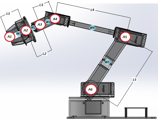
Figure 1:

In Figure 1 we can see the lengths ($L$) of the links as well as the weights ($W$) of the links considered that the center of mass is located at roughly the center of its length. The $a_{1}$ in the image is the ‘’load” being held by the arm, the $a_{2},a_{3},a_{4},a_{5}$ and $A6$ are the actuators (servos). To calculate the required torque ($T6$) of the $A6$ motor ($HS-805BB$ servo) we use the relation:

$$T_{6} =(L_{1}+L_{2}+L_{3}+L_{4}+L_{5})\ast A_{1}+(0.5\ast L_{1}+L_{2}+L_{3}+L_{4}+L_{5})\ast W_{1}$$

$$+(L_{2}+L_{3}+L_{4}+L_{5})\ast A_{2}+(0.5\ast L_{2}+L_{3}+L_{4}+L_{5})\ast W_{2}$$ (1)

$$+(L_{3}+L_{4}+L_{5})\ast A_{3}+(0.5\ast L_{3}+L_{4}+L_{5})\ast W_{3}$$

$$+(L_{4}+L_{5})\ast A_{4}+(0.5\ast L_{4}+L_{5})\ast W_{4}+(L_{5})\ast A_{5}+(0.5\ast L_{5})\ast W_{5}$$

To calculate the required torque ($T5$) of the $a_{5}$ motor ($HS-755HB$ servo):

$$T_{5} =(L_{1}+L_{2}+L_{3}+L_{4})\ast A_{1}+(0.5\ast L_{1}+L_{2}+L_{3}+L_{4})\ast W_{1}$$

$$+(L_{2}+L_{3}+L_{4})\ast A_{2}+(0.5\ast L_{2}+L_{3}+L_{4})\ast W_{2}$$ (2)

$$+(L_{3}+L_{4})\ast A_{3}+(0.5\ast L_{3}+L_{4})\ast W_{3}+(L_{4}+L_{5})\ast A_{4}+(0.5\ast L_{4}+L_{5})\ast W_{4}$$

The torque ($T4$) of the $a_{4}$ ($HS-645MG$ servo) is calculated:

$$T_{4} =(L_{1}+L_{2}+L_{3})\ast A_{1}+(0.5\ast L_{1}+L_{2}+L_{3})\ast W_{1}$$ (3)

$$+(L_{2}+L_{3})\ast A_{2}+(0.5\ast L_{2}+L_{3})\ast W_{2}+(L_{3})\ast A_{3}+(0.5\ast L_{3})\ast W_{3}$$

In a same manner the torque ($T3$) of the $a_{3}$ ($HS-225MG$ servo):

$$T_{3}=(L_{1}+L_{2})\ast A_{1}+(0.5\ast L_{1}+L_{2})\ast W_{1}+(L_{2})\ast A_{2}+(0.5\ast L_{2})\ast W_{2}$$ (4)

and finally the torque ($T2$) of the $a_{2}$ ($HS-422$ servo):

$$T_{2}=(L_{1})\ast A_{1}+(0.5\ast L_{1})\ast W_{1}$$ (5)

where:  $A_{2}=45.5g(HS-422)$, $A_{3}=31g(HS-225MG)$,  $A_{4}=55.2g(HS-645MG)+7g(ASB-24)=62.2g$, $A_{5}=110g(HS-755HB)+13g(ASB-201)=123g$, $A_{6}=197g(HS-805BB)+18g(ASB-204)=215g$ .

The weights are  $W_{1}=15.7g$ (Grip), $W_{2}=10g$ (Sensor Bracket), $W_{3}=9g$(Wrist Bracket), $W_{4}=10g$ (AT-04) +$6g$(ASB-06)+ $8g$ (HUB-08) =$24g$, $W_{5}=16g$ (ASB-205)+$15g$ ( ASB-203) = $31g$.

The lengths are : $L_{1}=2.8$ cm, $L_{2}=2.8$ cm, $L_{3}=2.85$cm, $L_{4}=18.73$ cm, $L_{5}=14.6$ cm.  If we replace the above, to the relations (1) - (5) and the weight of $A_{1}$ (load) is zero, the torques of the motors are:

• $T_{1}=0.021$ kg/cm

• $T_{2}=0.207$ kg/cm

• $T_{3}=0.511$ kg/cm

• $T_{4}=5.122$ kg/m

• $T_{5}=12.25$kg/cm

The nominal torques of the servo motors as given by the manufacturer are:

• $HS-422(T_{1})=4.1$ kg/cm

• $HS-225MG(T_{2})=4.8$ kg/cm

• $HS-645MG(T_{3})=9.6$ kg/cm

• $HS-755HB(T_{4})=13.2$ kg/cm

• $HS-805BB(T_{5})=24.7$ kg/cm

From the above, we can say that the arm is capable to lift its own weight because the nominal torques of the servos overlap the calculated torques with zero load ($A_{1}=0$).  Now If the load $A_{1}$ is set to be $100g$ the torques are:

• $T_{1}=0.3$ kg/cm

• $T_{2}=0.767$ kg/cm

• $T_{3}=1.356$ kg/cm

• $T_{4}=7.84$kg/cm

• $T_{5}=16.43$ kg/cm

We notice, if the load is $A_{1}=100g$, servos can cope. If we increase the weight at $A_{1}=300g$, then the calculated torques are:

• $T_{1}=0.86$ kg/cm

• $T_{2}=1.887$ kg/cm

• $T_{3}=3.04$ kg/cm

• $T_{4}=13.27$ kg/cm

• $T_{5}=24.79$ kg/cm

Hence the maximum weight the arm can lift is approximately ~300g because the calculated torques reach the nominal torques of the servos.

3.2 DOF (Degrees Of Freedom)

The arm has six actuators, one of which is to open and close the gripper, thus not being considered as a degree of freedom. The five rotational actuators have a degree of freedom each, with a result that the hole system has a total of five degrees of freedom. If we see the DOF of the arm through a mathematical point of view, the equation describing it is the Gruebler-Kutzbach equation and is expressed by the relation:

$$M=3\ast(n-1)-2\ast J_{1}-J_{2}$$

where $M$ is the DOF of the system, $n$ is the number of links including the base frame, $J_{1}$ is the number of joints that have one DOF, $J_{2}$ is the number of joints that have more than one DOF

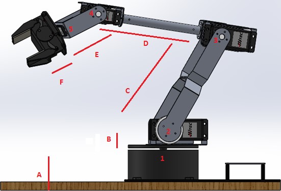
Figure 2:

In figure 2 we can see the links (A, B, C, D, E and F) and the joints (1, 2, 3, 4 and 5) of the arm. The number of the $J_{2}$ is zero because there is no joints of two DOF in the system.

Therefore:

$$M =3\ast(n-1)-2\ast J_{1}-J_{2}=3\ast 5-10\Rightarrow$$ (6)

$$M =5\text{ DOF}$$

3.3 Work Space

The work space of the arm is the space where the end effector can act. We compiled a code using MatLab for the 3D representation of the arm’s work space. In Figure 3 we can see the 3D presentation of the work space of the arm using the Robotics toolbox™(see [8], [Corke2011]. The top hemisphere (colored: yellow) is the actual work space of the arm and the bottom hemisphere (colored: blue) is a possible work space of the arm under certain circumstances. The diameter of the work area of the arm is approximately 40 cm .

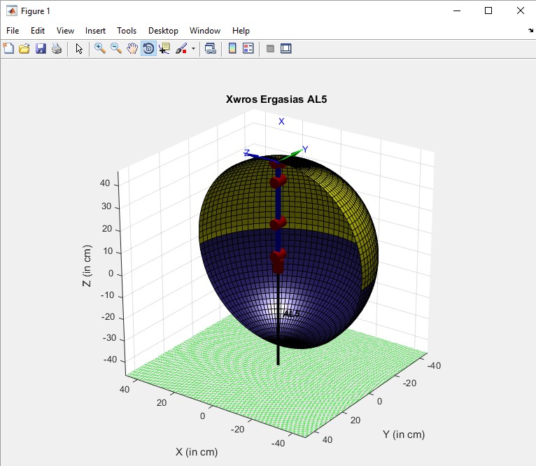
Figure 3:

3.4 Forward Kinematic

Forward Kinematics ([20], [12])refers to the use of kinematics equations of a robot to calculate the position of the end-effector from specified values for the joint parameters. The Denavit-Hartenberg parameters is the most common method being used to determine the Forward Kinematics analyses. Using this method we define the coordinate frames of the arm (Fig. 4), depending of the joints of mechanisms and then the D-H parameters table (Table 1) has been calculated

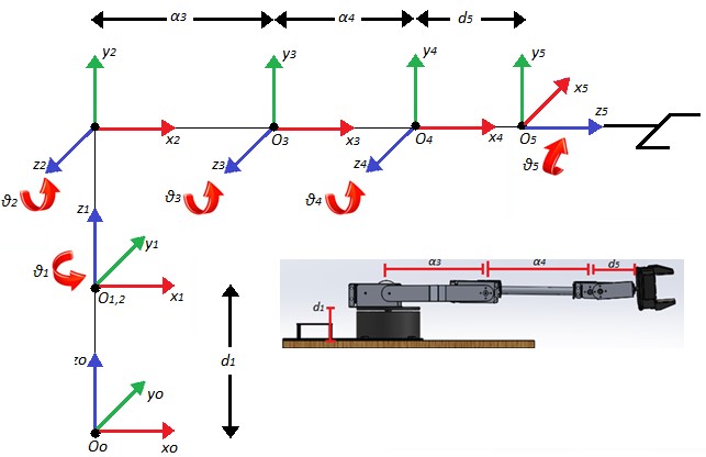
Figure 4:

Coordinate Frames has been defined with respect to D-H methodology where:

a_i is the length of the common perpendicular between points $O_{1,2}$ and $O_{4}$, $\ \ \alpha_{i}$ is the angle between axes $z_{i}$ and $z_{i-1},$ $d_{i}$ is the displacement distance of points $O_{0}-O_{1,2}$ and $O_{4}-O_{5},$ $\theta_{i}$ is the angle between axis $x_{i}$ and $x_{i-1}.$

$$\left[\begin{array}[c]{ccccc}\text{{Link i}}&\mathbf{a}_{i}&\mathbf{\alpha}_{i}&\mathbf{d}_{i}&\mathbf{\theta}_{i}\\ 1&0&0&d_{1}&\theta_{1}\\ 2&0&90^{o}&0&\theta_{2}\\ 3&\text{a}_{3}&0&0&\theta_{3}\\ 4&\text{a}_{4}&0&0&\theta_{4}(90^{o})\\ 5&0&-90^{o}&d_{5}&\theta_{5}\end{array}\right]$$ (7)

Using the D-H parameter table, homogeneous transformations matrixes are resulted

$$H_{0}^{1} =\begin{bmatrix}\cos\theta_{1}&-\sin\theta_{1}&0&0\\ \sin\theta_{1}&\cos\theta_{1}&0&0\\ 0&1&0&d_{1}\\ 0&0&0&1\end{bmatrix},\text{ \ \ \ \ }H_{1}^{2}=\begin{bmatrix}\cos\theta_{2}&-\sin\theta_{2}&0&0\\ 0&0&-1&0\\ \sin\theta_{2}&\cos\theta_{2}&0&0\\ 0&0&0&1\end{bmatrix}\text{\ \ , }$$ (8)

$$H_{2}^{3} =\begin{bmatrix}\cos\theta_{3}&-\sin\theta_{3}&0&\alpha_{3}\\ \sin\theta_{3}&\cos\theta_{3}&0&0\\ 0&1&0&0\\ 0&0&0&1\end{bmatrix}\text{\ }$$

$$H_{3}^{4} =\begin{bmatrix}\cos\theta_{4}&-\sin\theta_{4}&0&\alpha_{4}\\ \sin\theta_{1}&\cos\theta_{1}&0&0\\ 0&1&0&0\\ 0&0&0&1\end{bmatrix},\text{ \ \ \ \ }H_{4}^{5}=\begin{bmatrix}\cos\theta_{5}&-\sin\theta_{5}&0&0\\ 0&0&1&0\\ \sin\theta_{5}&\cos\theta_{5}&0&0\\ 0&0&0&1\end{bmatrix}$$

The multiplication of the matrixes (7)-(8) gives the table of the total homogeneous transformation, which is expressed:

$$H_{0}^{5}=H_{0}^{1}\ast H_{1}^{2}\ast H_{2}^{3}\ast H_{3}^{4}\ast H_{4}^{5}\begin{bmatrix}n_{x}&o_{x}&\alpha_{x}&d_{x}\\ n_{y}&o_{y}&\alpha_{y}&d_{y}\\ n_{z}&o_{z}&\alpha_{z}&d_{z}\\ 0&0&0&1\end{bmatrix}$$ (9)

where:

• $n=\left(n_{x},n_{y},n_{z}\right)^{T}$ is the vector representing the direction of the axis $\left(O_{1},x_{1}\right)$ in the coordinate system $\left(O_{0},x_{0},y_{0},z_{0}\right)$

• $o=\left(o_{x},o_{y},o_{z}\right)^{T}$ is the vector representing the direction of the axis $\left(O_{1},y_{1}\right)$ in the coordinate system $\left(O_{0},x_{0},y_{0},z_{0}\right)$

• $\alpha=\left(\alpha_{x},\alpha_{y},\alpha_{z}\right)^{T}$ is the vector representing the direction of the axis $\left(O_{1},z_{1}\right)$ in the coordinate system $\left(O_{0},x_{0},y_{0},z_{0}\right)$

• $d=\left(d_{x},d_{y},d_{z}\right)^{T}$ is the vector representing the direction of the axis $\left(O_{1},x_{1}\right)$ is the vector representing the joint’s position

where:

$n_{x}$= $((c_{1}c_{2}c_{3}-c_{1}s_{2}s_{3})c_{4}+(-c_{1}c_{2}s_{3}-c_{1}s_{2}c_{3})s_{4})c_{5}+s_{1}s_{5}$

$n_{y}$ = $((s_{1}c_{2}c_{3}-s_{1}s_{2}s_{3})c_{4}+(-s_{1}c_{2}s_{3}-s_{1}s_{2}c_{3})s_{4})c_{5}-c_{1}s_{5}$

$n_{z}$= $((s_{2}c_{3}+c_{2}s_{3})c_{4}+(-s_{2}s_{3}+c_{2}c_{3})s_{4})c_{5}$

$o_{x}$ = $-((c_{1}c_{2}c_{3}-c_{1}s_{2}s_{3})c_{4}+(-c_{1}c_{2}s_{3}-c_{1}s_{2}c_{3})s_{4})s_{5}-s_{1}c_{5}$

$o_{y}$ = $-((s_{1}c_{2}c_{3}-s_{1}s_{2}s_{3})c_{4}+(-s_{1}c_{2}s_{3}-s_{1}s_{2}c_{3})s_{4})s_{5}-c_{1}c_{5}$

$o_{z}$= $(c_{2}c_{3}-s_{2}s_{3})s_{4}-((-s_{2}c_{3}-c_{2}s_{3})c_{4}$

$\alpha_{x}$ = $-(c_{1}c_{2}c_{3}-c_{1}s_{2}s_{3})s_{4}+(-c_{1}c_{2}s_{3}-c_{1}s_{2}c_{3})c_{4}$

$\alpha_{y}$ = $-(s_{1}c_{2}c_{3}-s_{1}s_{2}s_{3})s_{4}+(-s_{1}c_{2}s_{3}-s_{1}s_{2}c_{3})c_{4}$

$\alpha_{z}$ = $(c_{2}c_{3}-s_{2}s_{3})c_{4}-(s_{2}c_{3}+c_{2}s_{3})s_{4}$

$d_{x}$ = $(-(c_{1}c_{2}c_{3}-c_{1}s_{2}s_{3})s_{4}+(-c_{1}c_{2}s_{3}-c_{1}s_{2}c_{3})c_{4})d_{5}+(c_{1}c_{2}c_{3}-c_{1}s_{2}s_{3})a_{4}+c_{1}c_{2}a_{3}$

$d_{y}$ = $(-(s_{1}c_{2}c_{3}-s_{1}s_{2}s_{3})s_{4}+(-s_{1}c_{2}s_{3}-s_{1}s_{2}c_{3})c_{4})d_{5}+(s_{1}c_{2}c_{3}-s_{1}s_{2}s_{3})a_{4}+s_{1}c_{2}a_{3}$

$d_{z}$ = $(-(s_{2}c_{3}+c_{2}s_{3})s_{4}+(-s_{2}s_{3}+c_{2}c_{3})c_{4})d_{5}+(s_{2}c_{3}-c_{2}s_{3})a_{4}+s_{2}a_{3}+d_{1}$ [6]

and  $c_{i}=\cos\theta_{i}$  , $s_{i}=\sin\theta_{i}$ .

3.5 Inverse Kinematic Analysis

In the Inverse kinematic ([20], [12])analysis we use the kinematics equations to find the desired position of the end-effector. In other words, forward kinematics uses the joint parameters to compute the configuration of a kinematic chain, and inverse kinematics reverses this calculation to determine the joint parameters that achieves a desired configuration. Calculation of the inverse kinematics problem is much more complex than forward kinematics, since there is no unique solution. In this project a geometric approach been used for solving the inverse kinematics problem. The complexity of the inverse kinematic problem increases with the number of nonzero link parameters and the geometric approach that used to solve the problem is simplest and more natural. The general idea of the geometric approach is to project the manipulator onto the $x_{0}$-$y_{0}$ plane (Figure 5) and solve a simple trigonometry problem to find $\theta_{1}$

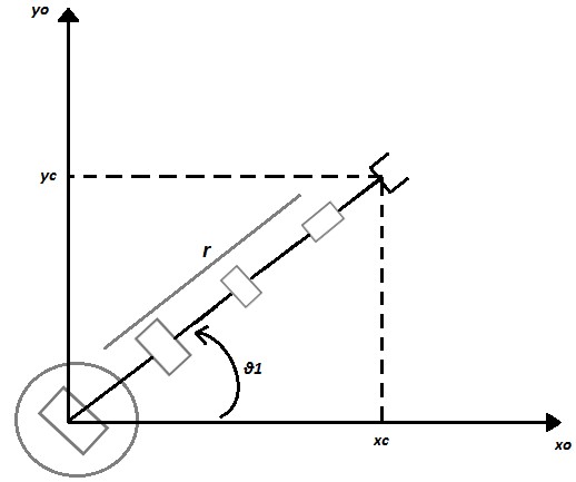
Figure 5:

From the projection we can see that

$$\theta_{1}=\text{atan}\left(\frac{y}{x}\right)$$ (10)

The distance from the base to the edge of the grip is $r$, therefore

$$r=\sqrt{x_{c}^{2}+y_{c}^{2}}$$ (11)

where

$$x_{c}=r\ast\cos(\theta_{1})\text{ \ and }y_{c}=r\ast\sin(\theta_{1})$$ (12)

A second projection of the manipulator is shown in Figure 6. From this projection we can see that the $A_{1}$ is :

$$A_{1}=\text{atan}\left(\frac{y}{x}\right)$$ (13)

The $A_{2}$ is :

$$A_{2}=\frac{\text{acos(}a_{3}^{2}-a_{4}^{2}+r^{2})}{a_{3}^{2}\ast r}$$ (14)

Therefore, the angle of the shoulder joint $\theta_{2}$ is :

$$\theta_{2}=A_{1}+A_{2}$$ (15)

The second solution of the angle $\theta_{2}$ is written:

$$\theta_{2}=A_{1}\pm A_{2}$$ (16)

The elbow joint corresponds to the angle $\theta_{3}$ which equals to :

$$\theta_{2}=\frac{\text{acos(}a_{3}^{2}+a_{4}^{2}+r^{2})}{a_{3}^{2}\ast a_{4}}$$ (17)

The relation between the angle $\psi$ (grip rotation) and the angles $\theta_{1},\theta_{2},\theta_{3}$ is written:

$$\theta_{4}=\psi-\theta_{2}-\theta_{3}$$ (18)

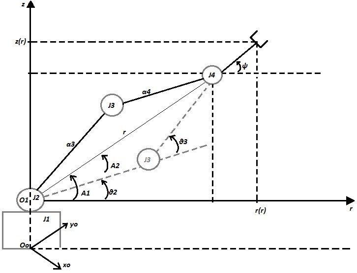
Figure 6:

From the geometric approach that analyzed above, the user will have complete control of the manipulator, controlling all six arm servos. When the user changes the angles $\theta_{2}$ and $\theta_{3}$, the angle $\theta_{4}$ will not change, thus not changing the point of the grip and its orientation. This is a consequence of the geometric approach (Figure 6). In other words, the three thrust mechanisms $\theta_{4}$ (rotation of the wrist), $\theta_{5}$ (grip rotation), $\theta_{6}$ (opening and closing of the grip) are not affected by the movement of angular movement mechanisms $\theta_{1}$ (base rotation), $\theta_{2}$(shoulder rotation) , $\theta_{3}$(elbow rotation), and the inverse . [6]

3.6
SolidWorks CAD-CAE

All the parts comprising the project have been measured and designed with usage of SolidWorks^© software. It’s a solid modeling computer-aided design (CAD) and computer-aided engineering (CAE) computer program. Users can see the full dimensionality (2D or 3D) of every part comprising the arm, as well as the material of every part. Additionally SolidWorks provides users with “countless” capabilities like measuring  parts, mass properties, motion study, collision check etc. In Figure 7, we can see the final 3D rendering of the arm.

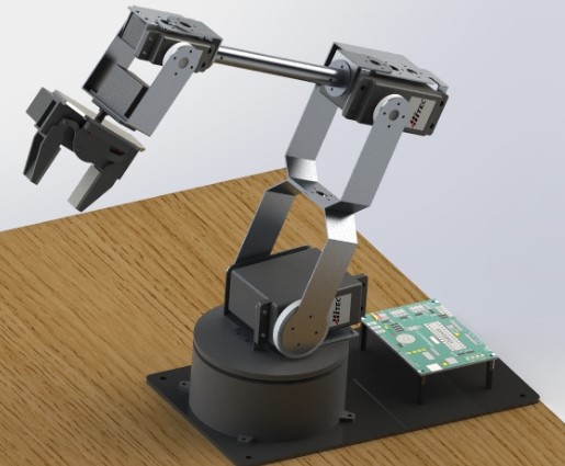
Figure 7:

4 Electrical-Electronic wiring

Communication compatibility between devices and the proper powering of these devices is important for the right operation of the project [11]. Once the correct devices have been selected based on their mechanical analysis, their electrical behavior should be analyzed in order to avoid encounter any communication or powering problems. In Figure 8 we can see the electrical diagram of the project. A current source ($220VAC/50Hz$ socket) feeds the computer’s power supply adapter ($18.5VDC/6.5A$) and another source feeds the BotBoarduino’s power supply adapter  ($6VDC/2.25A$). All servos are powered by the  BotBoarduino’s adapter, the IR sensor is powered by the computer’s USB cable ($5VDC/0.5A$),through the BotBoarduino’s regulator ($5VDC/1.5A$). The red (+ positive) and black (-negative) cables of the servos and IR sensor are for powering the devices, the yellow cable is for the communication with microcontroller ATMEGA328 and the computer through the USB cable (see [1],[3],[4],[9],[2],[13]).

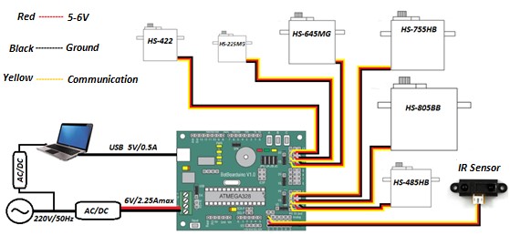
Figure 8:

4.1 Microcontroller Description

There are a lot of microcontroller boards in the market today with different functions, depending on the needs. The microcontroller board that was selected for this project is the BotBoarduino board because can give us the desired currents for the devices (servos and IR sensor) and can also split two sources of power for different powering needs. For example, in our project, servos are powered with 6VDC by bridging the jumper to the VS input and IR sensor is powered with 5VDC by bridging the jumper to the VL input. BotBoarduino is based on the ATMEGA328 microcontroller, it has a USB mini port that connects to a computer for programming the microcontroller. The LD29150DT50R regulator that BotBoarduino has onboard can power up to 1.5A current through the VL input. An external source of power (VS input) can also be connected onto the board, like the adapter (6V/2.25A) we use, for powering devices that need grater volts and amps, than the 5V/1.5A of VL input (see [3],[15],[9]).

4.2 Servomotors and IR Sensor

The angle of each servo controlled by the Pulse Width Modulation (PWM) value which is defined during programming. Each of the servo have an IC inside that can check the emitted PWM of the BotBoarduino and drive the servo to the desired position. Servos are powered by 6V DC by the adaptor through the BotBoarduino. The distance of IR sensor is measured by the Position Sensitive Detector (PSD) which then ‘’translate” the measured distance, through the IC of the sensor, to an output voltage. The greater the output voltage, the greater the distance. In the Figure 9 we can see the curve of the measured distance in relation with the output voltage. We can observe that the best accuracy region of the sensor is between the values of 10cm and 15cm. According to this, the distance between the sensor and the sorting objects must be between these values, for best accuracy (see [18],[3],[4]).

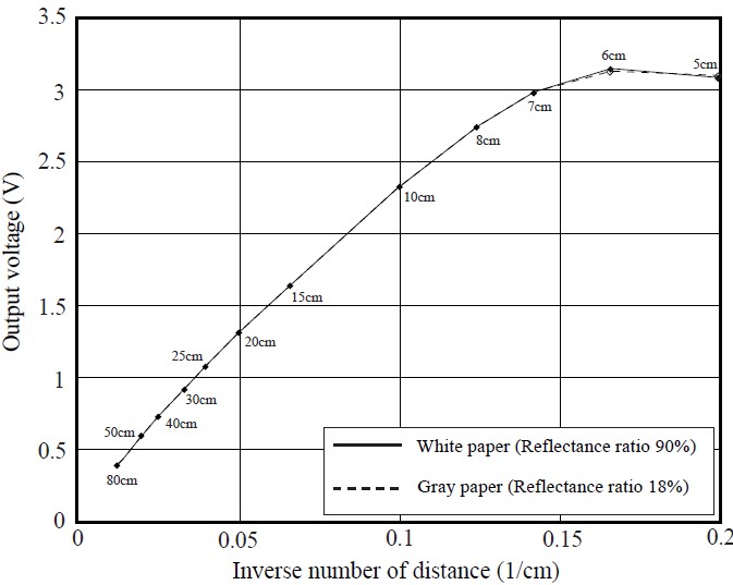
Figure 9:

4.3 Power Consumptions

The power consumption of the devices of the arm, is one of the most important topics in this study. The current consumed by the servos appears below:

• HS-485HB = 180mA

• HS-805BB = 830mA

• HS-755HB = 285mA

• HS-645MG = 450mA

• HS-225MG = 340mA

• HS-422 = 180mA

The sum of the consumption current of the servos is 2.265mA. The adaptor we selected for powering the servos gives us 2.250mA. The problem that occurs can be solved by moving one servo at a time. We achieve that in the programming. The communication current of each servo shown below:

• HS-485HB = 40mA

• HS-805BB = 40mA

• HS-755HB = 40mA

• HS-645MG = 40mA

• HS-225MG = 40mA

• HS-422 = 40mA

The powering current of IR sensor is 30mA and the communication current is 40mA. The sum of the communication currents of the servos plus the powering and communication currents of the sensor is 310mA. These currents powered by the USB cable (5V-0.5A) of the computer through the ‘’LD29150DT50R current regulator IC (5V-1.5A)” of the microcontroller. The regulator gives us a maximum of 1.5A current, which means that we can overlap the needs of 310mA (see [1],[13],[15], [9]).

5 Programming the Robotic Arm

In this section we provide the programming of the robotic arm. The software that have been used is the Arduino IDE (Integrated Development Environment). The programming language that he software supports are C and $C++$ (see [19],[10]). Arduino IDE supplies programmers with software libraries which provides them with many input or output procedures. A library, for example, can be loaded into the program by writing #include $<$math.h$>$ to the command line of Arduino IDE, this library is for the identification of the mathematical equations during programming. After the analysis of previous studies (Mechanical/Electrical-Electronic Engineering) we came up with four programs that show us the cooperation of the arm-sensor and its further applications within contemporary industrial forms of production.

5.1 Control cases

5.1.1 Autonomous Operation No.1

During the first autonomous operation, the arm takes the initial start position of the program, shown in Figure 10, then the arm takes the measuring position, according to the study that we have performed for the IR sensor (Fig. 11). As the arm reaches the measuring position, the IR sensor starts to collect distance measurements between the ‘’eye” of the sensor and the sorting area, as shown in the red circle in Figure 11. The distance between the sensor and the empty sorting area is set to 13.8 cm approximately. If the measurement is lower than 13.8 cm the sensor is set to recognize that an object is placed to the sorting area and the arm picks it up and puts it into the bucket

Figure 10:

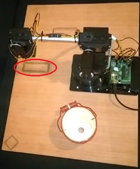
Figure 11:

The video for the first autonomous operation can be seen in this URL: www.youtube.com/watch?v=srE3x6y4jqU&feature=youtu.be

5.1.2 Autonomous Operation No.2

The initial start position and the measurement position is the same as the autonomous operation No.1. If the sensor measures between $<$13.8cm and $>$=10cm, recognizes that the object is ‘’short” (predefined measurements given). If the measurement is $>$greater than 10cm then the sensor recognizes that the object is ‘’tall”. The arm, then picks the object and places it to a predefined positioned bucket (Left for ‘’short” and Right for ‘’tall”).

The video for the second autonomous operation can be seen in this URL: www.youtube.com/watch?v=e8vaBb9g2A&feature=youtu.be

5.1.3 Autonomous Operation No.3

Third autonomous operation is almost the same  as the autonomous operation No.2. It differs in the placement of said objects. ‘’Short” object is placed to the predefined area, shown in Figure 12 and ‘’tall” object is placed to the predefined area, shown in Figure 13

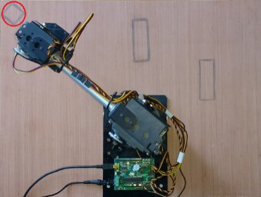
Figure 12:

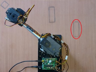
Figure 13:

The video for the third autonomous operation can be seen in this URL: www.youtube.com/watch?v=rFqdlcLnQ08

5.1.4 Manual Operation

The fourth program is the manual operation of the arm performed by a user with the keyboard of a computer loaded with said program. Users have full control of the arm manipulating each servo independently. Additionally users can see measurements of the sensor at the display of Arduino IDE.

The video for the manual operation can be seen in this URL:

www.youtube.com/watch?v=oFLjFvMqPjs&feature=youtu.be ([18],[19],[20])

6 Conclusions

A robot arm has been designed to cooperate with an infrared sensor for the identification of different sized objects and sorting them to predefined positions. Also the manual operation of the arm through computer’s keyboard is presented. The study is based on the three main axes that Mechatronics consist:

• Mechanical Engineering

• Electrical-Electronic Engineering

• Computer Science

In the case of mechanical engineering, we analyze the torque of servos, degrees of freedom and work space of the arm, mathematical modeling of forward and inverse kinematics and the CAD of the arm. Analysis of electrical-electronic engineering was important for the required powering of the devices (BotBoarduino, Servos, IR Sensor), for communication between devices and for the maximum efficiency of devices. Three promising experiments have been conducted concerning the use of autonomous operations and the manual operation of the arm , that can be applied to the industry, as well as to other working environments. The IR sensor can identify a variety of objects based on their height and to validate position and orientation information of the grasped object. The designed robotic arm might be an educational one, but the procedure and the methodology followed is similar for an industrial type of robotic arm. The next steps comprises, kinematic update to the arm, object reorientation routine, Dynamics and kinematics of the object to improve stable grasping.

References

- [1] ”Arduino,” 2005. [Online]. Available: www.arduino.cc. [Accessed 2016].
- [2] www.lynxmtion.com/images/html/build185.htm
- [3] ”Servo Motor Guide” http://www.anaheimautomation.com/manuals/forms/servomotor-guide.phpsthash.kpgbxS4k.dpbs
- [4] BALDOR ELECTRIC COMPANY, SERVO CONTROL FACTS http://www.baldor.com.
- [5] Barakat, A. N., Gouda, K. A. and Bozed, K. A., Kinematics analysis and simulation of a robotic arm using MATLAB, 2016 4th International Conference on Control Engineering Information Technology (CEIT), IEEE, 2016, pp. 1-5
- [6] Benson, C. Robot Arm Torque Tutorial http://www.robotshop.com/blog/en/robot-arm-torque-tutorial- 7152, 2016
- [7] Corke P., Robotics, vision and control. Fundamental algorithms in MATLAB. Berlin: Springer, 2011.
- [8] Corke, P., ”A robotics toolbox for MATLAB”, IEEE Robot. Automat. Mag. Vol. 3(1), pp. 24-32.
- [9] F. Chips, FT232R Datasheet , Future Technology Devices International Ltd., 2015.
- [10] B. Eckel, Thinking in C++, Volume 1, 2nd Edition, Upper Saddle River, New Jersey 07458 : Prentice Hall , January 13, 2000
- [11] Behrouz A. Forouzan, Data Communications And Networking Second Edition,, Higher Education, 2000.
- [12] Graig J (2017), ”Introduction to Robotics: Mechanics and Control (4th Edition)” Pearson.
- [13] D. Hart, Power Electronics, McGraw-Hill, New York, NY 10020, 2011.
- [14] Khanna, P., Singh, K., Bhurchandi, K. M., and Chiddarwar, S. Design analysis and development of low cost underactuated robotic hand. In 2016 IEEE International Conference on Robotics and Biomimetics (ROBIO) (Dec 2016), pp. 2002-2007.
- [15] LD29150 Datasheet, STMicroelectronics, 2013.
- [16] Lee, D. H., Park, J. H., Park, S. W., Baeg, M. H., and Bae, J. H. Kitech-hand: A highly dexterous and modularized robotic hand. IEEE-ASME Transactions on Mechatronics 22, 2 (April 2017), 876-887.
- [17] R. A. Serway, Physics for Scientists and Engineers. 6th Ed., Brooks Cole, 2003.
- [18] Sharp Corporation. GP2Y0A21YK0F Datasheet, 2006
- [19] Souli J., C++ Language Tutorial, cplusplus.com, 2007
- [20] Mark W. Spong, Robot Modeling and Control 1st Edition, John Wiley and Sons, 2005.