Variance optimal hedging with application to Electricity markets

Abstract

In this article, we use the mean variance hedging criterion to value contracts in incomplete markets. Although the problem is well studied in a continuous and even discrete framework, very few works incorporating illiquidity constraints have been achieved and no algorithm is available in the literature to solve this problem. We first show that the valuation problem incorporating illiquidity constraints with a mean variance criterion admits a unique solution. Then we develop two Least Squares Monte Carlo algorithms based on the dynamic programming principle to efficiently value these contracts: in these methods, conditional expectations are classically calculated by regression using a dynamic programming approach discretizing the control. The first algorithm calculates the optimal value function while the second calculates the optimal cash flow generated along the trajectories. In a third part, we give the example of the valuation of a load curve contract coming from energy markets. In such contracts, incompleteness comes from the uncertainty of the customer’s load that cannot be hedged and very tight illiquity constraints are present. We compare strategies given by the two algorithms and by some closed formula ignoring constraints and we show that hedging strategies can be very different. A numerical study of the convergence of the algorithms is also given.

Keywords: Monte-Carlo methods, mean variance hedging, energy, finance

MSC2010: Primary 65C05, 60J60; Secondary 60J85, 60H35.

1 Introduction

Since the deregulation of the energy market in the 1990, spot and future contract on electricity are available in many countries. Because electricity cannot be stored easily and because balance between production and consumption has to be checked at every moment, electricity prices exhibit spikes when there is a high demand or a shortage in production. These high variations in the price lead to fat tails of the distribution of the log return of the price and Gaussian models for example fail to reproduce this feature. Many models have been developed to reproduce the statistical features of electricity prices as shown in aid2015electricity leading to incomplete market modeling. However even in the case of a Gaussian model there are many sources of friction and incompleteness on energy market: The first is the liquidity of hedging products available on the market. Large change in position leads to change in prices and then the hypothesis of an exogenous price model is not valid anymore. In order to limit their impacts on price, risk managers spread in time their selling/buying orders. A realistic hedging strategy has to take these constraints into account. Besides due to the bid ask spread which is already a source of friction and due to the inaccuracy of the models used, hedging is only achieved once a week or twice a month so that the hypothesis of a continuous hedge is far from being satisfied. Further, on electricity market, some contracts are not only dependent on the prices. For example a retailer has to provide the energy to fit a load curve which is uncertain mainly due to its sensitivity to temperature and business activity so that a perfect hedge of such contracts is impossible.
The literature on the effect of a discrete hedging has been theoretically studied in complete markets in zhang1999couverture, bertsimas2000time, hayashi2005evaluating. In the case of incomplete markets with some jumps some results about the hedging error due to the discrete hedging dates can be found in tankov2009asymptotic.
The Leland proxy (leland1985option) was the first proposed to take into account discrete hedging dates and transaction costs. One theoretical result obtained using a Black Scholes model gives that when proportional transaction costs decrease with the number of interventions $n$ proportionally to $n^{-\alpha}$ with $\alpha\in]0,\frac{1}{2}]$, the hedging error goes to zero in probability when a call is valued and hedged using the Black Scholes formula with a modified volatility.
Following this first work, a huge literature on transaction cost has developed. For example, the case $\alpha=0$ corresponding to the realistic case where the transaction cost are independent on the frequency to the hedge has been dealt in kabanov1997leland, pergamenshchikov2003limit, denis2010mean, soner1995there.
The case of a limited availability of hedging products has not been dealt theoretically nor numerically so far in the literature to our knowledge. Most of the research currently focuses on developing some price impact features to model the liquidation of a position (see for example gatheral2010no) instead of imposing some depth limits.
In order to get realistic hedging strategies and because of all the sources of incompleteness, a risk criterion has to be used to define the optimal hedging strategy of the contingent claim with a given payoff at maturity date $T$. In this article we use a mean variance strategy to define this optimal policy taking into account the fact that hedging is achieved at discrete dates, that transaction costs are present and that the orders are limited in volume at each date.
Mean variance hedging is theoretically well studied in the literature. The first paper on the subject (duffie1991mean) in a continuous setting was followed by a many articles on the subject. As we mentioned before, the continuous assumption is not satisfied in practice and an approach taking into account some discrete dates of hedging was proposed in follmer1988hedging. As in the continuous case, some attention has been focus on finding semi-explicit formula for hedging strategies (see goutte2014variance and references inside).
In the general case, with transaction costs and constraints on hedging position, there are no explicit solutions so it is necessary to rely on numerical methods. There are no algorithms proposed to solve this problem: Mean variance algorithm without friction and based on tree resolution have been developed by vcerny2004dynamic but tree methods are only effective in very low dimension. The main contribution of this article is to propose two algorithms based on a dynamic programming approach to solve this problem in the general case. Using Monte Carlo methods and relying on regressions (Least Square Monte Carlo) to calculate the conditional expectations, we propose a first version calculating the function value recursively in time by discretizing the command and the amount invested in risky assets. A second version is proposed tracking the optimal cash flows generated by the strategy using a methodology similar to the one used in longstaff2001valuing. The use of the Monte Carlo method permits to have flexible algorithm permitting to solve the problem in multi dimension with respect to the number of hedging products.
The article has the following structure:
In a first part, in a general setting using the previous work of schweizer1995variance, motoczynski2000multidimensional and beutner2007mean, we show that the problem admits a solution in a general case.
In a second part we develop the two versions of the algorithm.
In a third part, we focus on the problem of an energy retailer that needs to hedge an open position corresponding to a stochastic load curve by trading future contracts. Using a Gaussian one factor HJM model for the future curve and an Ornstein Ulhenbeck model for the load curve, we show that on electricity market, taking into account the discrete hedge and the limited orders has a high impact on the optimal strategy. We also compare numerically the two versions of the algorithm and study some convergence properties on one test case.
In the whole paper we only consider the case with only one hedging instrument. There is no technical problem to deal with more hedging instruments but numerical experiments are easier with only one asset due to the different discretizations used in the proposed algorithms.

2 Mean variance hedging in a general framework

In this section we suppose that $(\Omega,{\cal F},({\cal F}_{t})_{t\in\left[0,T\right]})$ is a filtered probability space. We define a set of trading dates $\mathcal{T}=\{t_{0}=0,t_{1},\ldots,t_{N-1},t_{N}=T\}$ and we suppose that $(S_{t})_{t_{0}.t_{N}}$ is an almost surely positive hedging product $(S_{t})_{t_{0}.t_{N}}$, square integrable so that $\mathbb{E}\left[S_{t}^{2}\right]<\infty$ and adapted so that $S_{t}$ is ${\cal F}_{t}$-measurable for $t=t_{0},\ldots,t_{N}$.
Further we suppose that the risk free rate is zero so that a bond has always a value of $1$.
We suppose that the contingent claim $H\in{\cal L}^{2}(P)$ is a ${\cal F}_{T}$-measurable random variable. In the case of a European call option on an asset $S_{t}$ with strike $K$ and maturity $T$, $H(\omega)=(S_{T}(\omega)-K)^{+}$.
In this paper we are only interested in self-financing strategies with limited orders, so with bounded controls. Extending motoczynski2000multidimensional, beutner2007mean’s definition, we define:

Definition 2.1.

A $(\bar{m},\bar{l})$ self-financing strategy ${\cal V}=({\cal V}_{t_{i}})_{i=0,\ldots,N-1}$ is a pair of adapted process $(m_{t_{i}},l_{t_{i}})_{i=0,\ldots,N-1}$ defined for $(\bar{m},\bar{l})\in(0,\infty)\times(0,\infty)$ such that:

• $0\leq m_{t_{i}}\leq\bar{m},\quad 0\leq l_{t_{i}}\leq\bar{l}\quad\quad P.a.s.\quad\forall i=0,\ldots,N-1$,

• $m_{t_{i}}l_{t_{i}}=0\quad P.a.s.\quad\forall i=0,\ldots,N-1$.

In this definition $m_{t}$ corresponds to the number of shares sold at date $t$, and $l_{t}$ the number of shares bought at this date.

Remark 2.1.

The strategies defined in motoczynski2000multidimensional and beutner2007mean do not impose that $m_{t}l_{t}=0$ so a buy and sell control could happen at the same given date.

We note $\Theta^{(\bar{m},\bar{l})}$ the set of $(\bar{m},\bar{l})$ self-financing strategy and with the notation $\nu=(m,l)$ for $\nu\in\Theta^{(\bar{m},\bar{l})}$.
We consider a model of proportional cost, so that an investor buying a share at date $t$ pays $(1+\lambda)S_{t}$ and an investor selling this share only receives $(1-\lambda)S_{t}$. Assuming that there are no transaction costs on the last date $T$, the terminal wealth of an investor with initial wealth $x$ is given by:

$$x-\sum_{i=0}^{N-1}(1+\lambda)l_{t_{i}}S_{t_{i}}+\sum_{i=0}^{N-1}(1-\lambda)m_{t_{i}}S_{t_{i}}+\sum_{i=0}^{N-1}l_{t_{i}}S_{t_{N}}-\sum_{i=0}^{N-1}m_{t_{i}}S_{t_{N}}.$$ (2.1)

Remark 2.2.

The transaction costs on the last date $T$ are related to the nature of the contract. In the case of a pure financial contract, the investor sells the asset and then some transaction costs have to be paid to clear the final position. On energy market for example, the contract is often associated to physical delivery and no special fees are to be paid. Besides on these markets, futures markets are rather illiquid and the associated transaction costs are large whereas spot markets are much more liquid with transaction costs that can be neglected.

As in motoczynski2000multidimensional, beutner2007mean, we define the risk minimal strategy minimizing the ${\cal L}^{2}$ risk of the hedged portfolio supposing that the hedger liquidates her entire accumulated position at date $T$:

Definition 2.2.

A $(\bar{m},\bar{l})$ self-financing strategy $\hat{\cal V}=(\hat{m},\hat{l})$ is global risk minimizing for the contingent claim $H$ and the initial capital $x$ if:

$$\hat{\cal V}= \mbox{\rm arg}\min_{{\cal V}=(m,l)\in\Theta^{(\bar{m},\bar{l})}}\mathbb{E}\left[(H-x+\sum_{i=0}^{N-1}(1+\lambda)l_{t_{i}}S_{t_{i}}-\right.$$

$$\left.\sum_{i=0}^{N-1}(1-\lambda)m_{t_{i}}S_{t_{i}}-\sum_{i=0}^{N-1}l_{t_{i}}S_{t_{N}}+\sum_{i=0}^{N-1}m_{t_{i}}S_{t_{N}})^{2}\right].$$ (2.2)

In order to show the existence of solution to problem (2.2), we need to make some assumptions on the prices as in motoczynski2000multidimensional, beutner2007mean:

Assumption 2.3.

The price process $S=(S_{t_{i}})_{i=0,\ldots,N}$ is such that a constant $K_{1}>0$ satisfies:

$$\mathbb{E}\left[\frac{S_{t_{i}}^{2}}{S_{t_{i-1}}^{2}}|{\cal F}_{t_{i-1}}\right]\leq K_{1},\quad P.a;s.,\quad\forall i=1,\ldots,N.$$

Assumption 2.4.

The price process $S=(S_{t_{i}})_{i=0,\ldots,N}$ is such that a constant $K_{2}>0$ satisfies:

$$\mathbb{E}\left[\frac{S_{t_{i-1}}^{2}}{S_{t_{i}}^{2}}|{\cal F}_{t_{i-1}}\right]\leq K_{2},\quad P.a.s.,\quad\forall i=1,\ldots,N.$$

Assumption 2.5.

The price process $S=(S_{t_{i}})_{i=0,\ldots,N}$ is such that a constant $\delta\in(0,1)$ satisfies:

$$(\mathbb{E}\left[S_{t_{i}}|{\cal F}_{t_{i-1}}\right])^{2}\leq\delta E\left[S_{t_{i}}^{2}|{\cal F}_{t_{i-1}}\right],\quad P.a.s.,\quad\forall i=1,\ldots,N.$$

We introduce the gain function:

Definition 2.6.

For ${\cal V}\in\Theta^{(\bar{m},\bar{l})}$, we define the gain functional $G_{T}:\Theta^{(\bar{m},\bar{l})}\longrightarrow{\cal L}^{2}$ by

$$G_{T}({\cal V}):=-\sum_{i=0}^{N-1}(1+\lambda)l_{t_{i}}S_{t_{i}}+\sum_{i=0}^{N-1}l_{t_{i}}S_{T}+\sum_{i=0}^{N-1}(1-\lambda)m_{t_{i}}S_{t_{i}}-\sum_{i=0}^{N-1}m_{t_{i}}S_{T}$$ (2.3)

In order to show that our problem is well-defined, we want to show that $G_{T}(\Theta^{(\bar{m},\bar{l})})$ is closed in ${\cal L}^{2}$. As in motoczynski2000multidimensional, beutner2007mean, we have to introduce another functional $\tilde{G}_{T}({\cal V}):\Theta^{(\bar{m},\bar{l})}\longrightarrow{\cal L}^{2}\times{\cal L}^{2}\times{\cal L}^{2}$ defined by:

$$\tilde{G}_{T}({\cal V}):=\left(\begin{array}[]{l}-\sum_{i=0}^{N-1}(1+\lambda)l_{t_{i}}S_{t_{i}}\\ \sum_{i=0}^{N-1}(1-\lambda)m_{t_{i}}S_{t_{i}}\\ \sum_{i=0}^{N-1}(l_{t_{i}}-m_{t_{i}})S_{T}.\end{array}\right)$$ (2.7)

Proposition 2.7.

Under assumptions 2.3,2.4,2.5, $\tilde{G}_{T}(\Theta^{(\bar{m},\bar{l})})$ is a closed bounded convex set of ${\cal L}^{2}\times{\cal L}^{2}\times{\cal L}^{2}$.

Proof.

The convexity of the set is due to the linearity of the $\tilde{G}_{T}$ operator. Because of the boundedness of $(l_{t_{i}},m_{t_{i}})$, $i=0,N-1$ and the $(S_{t_{i}})_{i=0,N}$ square integrability, we have that $\tilde{G}_{T}(\Theta^{(\bar{m},\bar{l})})$ is bounded in ${\cal L}^{2}\times{\cal L}^{2}\times{\cal L}^{2}$.
In order to prove the closedness of $\tilde{G}_{T}(\Theta^{(\bar{m},\bar{l})})$, we suppose that we have a sequence $({\cal V}^{n})=(m^{n}_{t_{i}},l^{n}_{t_{i}})_{i=0,N-1}\in\Theta^{(\bar{m},\bar{l})}$ such that $\tilde{G}_{T}({\cal V}^{n})$ converges in ${\cal L}^{2}\times{\cal L}^{2}\times{\cal L}^{2}$.
Using assumption 2.5 and lemma 5.3 in motoczynski2000multidimensional, we get that for $i=0,\ldots,N-1$, there exist $l_{t_{i}}^{\infty}$, $m_{t_{i}}^{\infty}$ ${\cal F}_{t_{i}}$-adapted such that $l_{t_{i}}^{\infty}S_{t_{i}}\in{\cal L}^{2}$, $m_{t_{i}}^{\infty}S_{t_{i}}\in{\cal L}^{2}$ and

$$l_{t_{i}}^{n}S_{t_{i}}\xrightarrow{{\cal L}^{2}}l_{t_{i}}^{\infty}S_{t_{i}},$$

$$m_{t_{i}}^{n}S_{t_{i}}\xrightarrow{{\cal L}^{2}}m_{t_{i}}^{\infty}S_{t_{i}},$$

so that

$$-\sum_{i=0}^{N-1}(1+\lambda)l_{t_{i}}^{n}S_{t_{i}}\xrightarrow{{\cal L}^{2}}-\sum_{i=0}^{N-1}(1+\lambda)l_{t_{i}}^{\infty}S_{t_{i}},$$

$$\sum_{i=0}^{N-1}(1-\lambda)m_{t_{i}}^{n}S_{t_{i}}\xrightarrow{{\cal L}^{2}}\sum_{i=0}^{N-1}(1-\lambda)m_{t_{i}}^{\infty}S_{t_{i}}.$$

Using Lemma 5 in beutner2007mean based on assumption2.3, we get that $l^{n}_{t_{i}}S_{T}$ converges weakly to $l^{\infty}_{t_{i}}S_{T}$, and $m^{n}_{t_{i}}S_{T}$ converges weakly to $m^{\infty}_{t_{i}}S_{T}$, for $i=0,\ldots,N-1$ such that

$$\sum_{i=0}^{N-1}(l_{t_{i}}^{n}-m_{t_{i}}^{n})S_{T}\xrightarrow{\text{weak}}\sum_{i=0}^{N-1}(l_{t_{i}}^{\infty}-m_{t_{i}}^{\infty})S_{T}.$$

Using the fact that strong and weak limit coincide in ${\cal L}^{2}$, we get that the limit of $\tilde{G}_{T}({\cal V}^{n})$ is $\tilde{G}_{T}({\cal V}^{\infty})$ with ${\cal V}^{\infty}=(m^{\infty},l^{\infty})\in{\cal L}^{2}\times{\cal L}^{2}$.
We still have to show that $l_{t_{i}}^{\infty}$, $m^{\infty}_{t_{i}}$ respect the constraints: First using assumption2.4 and the tower property of conditional expectation, we have

$$\mathbb{E}\left[\frac{1}{S_{t_{i}}^{2}}\right]\leq\frac{K_{2}^{i}}{S_{0}^{2}}<\infty,\forall i=0,\ldots,N.$$ (2.8)

Suppose for example that there exist $\epsilon>0$ and $i<N$ such that $l_{t_{i}}^{\infty}(\omega)>\bar{l}+\epsilon$ for $\omega$ in a set ${\cal A}$ with a non zero measure $\tilde{\cal A}$. Then,

$$(\bar{l}+\epsilon)\tilde{\cal A}\leq E\left[l^{\infty}_{t_{i}}1_{{\cal A}}\right],$$

$$= E\left[(l^{\infty}_{t_{i}}-l^{p}_{t_{i}})1_{{\cal A}}\right]+E\left[l^{p}_{t_{i}}1_{{\cal A}}\right],$$

$$\leq E\left[(l^{\infty}_{t_{i}}S_{T}-l^{p}_{t_{i}}S_{T})1_{{\cal A}}\frac{1}{S_{T}}\right]+\bar{l}\tilde{\cal A}.$$

Then using (2.8) we know that $1_{{\cal A}}\frac{1}{S_{T}}$ is in ${\cal L}^{2}$ so using the weak convergence of $l^{p}_{t_{i}}S_{T}$ towards $l^{\infty}_{t_{i}}S_{T}$ and letting $p$ go to infinity gives the contradiction.
The same type of calculation shows that $l^{\infty}_{t_{i}}\geq 0$, $0\leq\mathrm{m}^{\infty}_{t_{i}}\leq\bar{m}$.
At last it remains to show that $l^{\infty}m^{\infty}=0$. Suppose for example that there exist $\epsilon>0$ and $i<N$ such that $l_{t_{i}}^{\infty}(\omega)m_{t_{i}}^{\infty}(\omega)>\epsilon$ for $\omega$ in a set ${\cal A}$ with a non zero measure $\tilde{\cal A}$.
Using the fact that $l_{t_{i}}^{n}m_{t_{i}}^{n}=0$, $\frac{m_{t_{i}}^{n}1_{{\cal A}}}{S_{t_{i}}}\in{\cal L}^{2}$ and Cauchy Schwartz:

$$\epsilon\tilde{\cal A}\leq E\left[l_{t_{i}}^{\infty}m_{t_{i}}^{\infty}1_{{\cal A}}\right],$$

$$= \mathbb{E}\left[(S_{t_{i}}m_{t_{i}}^{\infty}-S_{t_{i}}m_{t_{i}}^{n})\frac{l_{t_{i}}^{\infty}1_{{\cal A}}}{S_{i}}\right]+\mathbb{E}\left[(S_{t_{i}}l_{t_{i}}^{n}-S_{t_{i}}l_{t_{i}}^{\infty})\frac{m_{t_{i}}^{n}1_{{\cal A}}}{S_{t_{i}}}\right]$$

$$\leq |\mathbb{E}\left[(S_{t_{i}}m_{t_{i}}^{\infty}-S_{t_{i}}m_{t_{i}}^{n})\frac{l_{t_{i}}^{\infty}1_{{\cal A}}}{S_{i}}\right]|+||S_{t_{i}}l_{t_{i}}^{n}-S_{t_{i}}l_{t_{i}}^{\infty}||_{{\cal L}^{2}}\bar{m}\tilde{\cal A}\frac{K_{2}^{0.5i}}{S_{0}}.$$

Letting $n$ go to infinity, and using the strong/weak convergence property we get the contradiction. ∎

We are now in position to give the existence and uniqueness theorem:

Theorem 2.8.

Under assumptions 2.3, 2.4, 2.5, the minimization problem (2.2) admits a unique solution.

Proof.

First we show that $G_{T}(\Theta^{(\bar{m},\bar{l})})$ is a closed bounded convex set in ${\cal L}^{2}$. Convexity and boundedness are straightforward. Suppose that we have a sequence $({\cal V}^{n})=(m^{n}_{t_{i}},l^{n}_{t_{i}})_{i=0,N-1}\in\Theta^{(\bar{m},\bar{l})}$ such that $G({\cal V}^{n})$ converges in ${\cal L}^{2}$. $\tilde{G}_{T}(\Theta^{(\bar{m},\bar{l})})$ being a bounded closed convex set due to proposition 2.7, it is weakly closed, and we can extract a sub sequence ${\cal V}^{p}$ such that $\tilde{G}_{T}({\cal V}^{p})$ converges weakly to $\tilde{G}_{T}({\cal V}^{\infty})$ with ${\cal V}^{\infty}\in\Theta^{(\bar{m},\bar{l})}$. Then by linearity $G_{T}({\cal V}^{p})$ converges weakly to $G_{T}({\cal V}^{\infty})$ and due to the fact that weak and strong limit coincide, we get that $G_{T}({\cal V}^{p})$ converges strongly to $G_{T}({\cal V}^{\infty})$ giving the closedness of $G_{T}(\Theta^{(\bar{m},\bar{l})})$.
As a result, the solution of the minimization problem exists, is unique and corresponds to the projection of $H$ on $G_{T}(\Theta^{(\bar{m},\bar{l})})$ in ${\cal L}^{2}$. ∎

3 Algorithms for mean variance hedging

In this section we suppose that the process is Markov and that the payoff $H$ is a function of the asset value at maturity only to simplify the presentation for the Monte Carlo methods proposed. In a first section we give two algorithms based on dynamic programming and regressions to calculate the solution of the problem (2.2). In a second part we detail the resolution for one algorithm using some specific regressors and discretizing commands and stocks.

3.1 Some dynamic programming algorithms

We introduce the global position $\nu=(\nu_{i})_{i=0,\ldots,N-1}$ with:

$$\nu_{i}=\sum_{j=0}^{i}(m_{t_{j}}-l_{t_{j}}),\forall i=0,\ldots,N-1.$$

Using the property that $m_{t_{i}}l_{t_{i}}=0$ for all $i=0,\ldots,N-1$, we get that $|\nu_{i}-\nu_{i-1}|=l_{t_{i}}+m_{t_{i}}$ with the convention that $\nu_{-1}=0$ so that the gain functional can rewritten as:

$$G_{T}({\cal V})=\hat{G}_{T}(\nu)=x-\sum_{i=0}^{N-1}\lambda|\Delta\nu_{i-1}|S_{t_{i}}+\sum_{i=0}^{N-1}\nu_{i}\Delta S_{i},$$

where $\Delta S_{i}=S_{t_{i+1}}-S_{t_{i}}$, $\Delta\nu_{i}=\nu_{i+1}-\nu_{i}$.
We then introduce $\hat{\Theta}^{(\bar{m},\bar{l})}$ the set of adapted random variable $(\nu_{i})_{i=0,\ldots,N-1}$ such that

$$-\bar{m}\leq\nu_{i}-\nu_{i-1}\leq\bar{l},\quad\forall i=1,\ldots,N-1.$$

The problem (2.2) can be rewritten as done in schweizer1995variance finding $\hat{\nu}=(\hat{\nu}_{i})_{i=0,\ldots,N-1}$ satisfying:

$$\hat{\nu}= \mbox{\rm arg}\min_{\nu\in\hat{\Theta}^{(\bar{m},\bar{l})}}\mathbb{E}\left[\big{(}H-x-\hat{G}_{T}(\nu)\big{)}^{2}\right].$$ (3.1)

We introduce the spaces $K_{i}$, $i=0,\ldots,N$ of the ${\cal F}_{t_{i}}$-measurable and square integrable random variables. We define for $i\in 0,\ldots,N$, $V_{i}\in K_{i}$ as:

$$V_{N}= H,$$

$$V_{i}= \mathbb{E}\left[H-\sum_{j=i}^{N-1}\nu_{j}\Delta S_{j}+\lambda\sum_{j=i}^{N-1}|\Delta\nu_{j-1}|S_{t_{j}}\quad|{\cal F}_{t_{i}}\right],\forall i=0,\ldots,N-1.$$ (3.2)

Then we can prove the following proposition:

Proposition 3.1.

The problem (3.1) can be rewritten as:

$$\hat{\nu}= \mbox{\rm arg}\min_{\nu\in\hat{\Theta}^{(\bar{m},\bar{l})}}\mathbb{E}\left[\left(V_{N}-\nu_{N-1}\Delta S_{N-1}+\lambda|\Delta\nu_{N-2}|S_{t_{N-1}}-V_{N-1}\right)^{2}\right]+$$

$$\sum_{i=2}^{N-1}\mathbb{E}\left[\left(V_{i}+\lambda|\Delta\nu_{i-2}|S_{t_{i-1}}-\nu_{i-1}\Delta S_{i-1}-V_{i-1}\right)^{2}\right]+$$

$$\mathbb{E}\left[\left(V_{1}+\lambda|\nu_{0}|S_{t_{0}}-\nu_{0}\Delta S_{0}-x\right)^{2}\right].$$ (3.3)

Proof.

$$\mathbb{E}\left[(H-x-\hat{G}_{T}(\nu))^{2}\right]= E\left[\big{(}\left(V_{N}-\nu_{N-1}\Delta S_{N-1}+\lambda|\Delta\nu_{N-2}|S_{t_{N-1}}-V_{N-1}\right)+\right.$$

$$\sum_{i=2}^{N-1}\left(V_{i}+\lambda|\Delta\nu_{i-2}|S_{t_{i-1}}-\nu_{i-1}\Delta S_{i-1}-V_{i-1}\right)+$$

$$\left.\left(V_{1}+\lambda|\nu_{0}|S_{t_{0}}-\nu_{0}\Delta S_{0}-x\right)\big{)}^{2}\right]$$ (3.4)

Due to the definition (3.1), we have that

$$E\left[V_{i}+\lambda|\Delta\nu_{i-2}|S_{t_{i-1}}-\nu_{i-1}\Delta S_{i-1}-V_{i-1}|{\cal F}_{t_{i-1}}\right]=0,\forall i=1,\ldots,N,$$ (3.5)

so that

$$\mathbb{E}\left[(H-x-\hat{G}_{T}(\nu))^{2}\right]= \mathbb{E}\left[\mathbb{E}\left[\left(V_{N}-\nu_{N-1}\Delta S_{N-1}+\lambda|\Delta\nu_{N-2}|S_{t_{N-1}}-V_{N-1}\right)^{2}|{\cal F}_{t_{N-1}}\right]\right]+$$

$$\mathbb{E}\left[\sum_{i=2}^{N-1}\left(V_{i}+\lambda|\Delta\nu_{i-2}|S_{t_{i-1}}-\nu_{i-1}\Delta S_{i-1}-V_{i-1}\right)^{2}+\right.$$

$$\left.\left(V_{1}+\lambda|\nu_{0}|S_{t_{0}}-\nu_{0}\Delta S_{0}-x\right)^{2}\right]$$

and iterating the process gives

$$\mathbb{E}\left[(H-x-\hat{G}_{T}(\nu))^{2}\right]= \mathbb{E}\left[\left(V_{N}-\nu_{N-1}\Delta S_{N-1}+\lambda|\Delta\nu_{N-2}|S_{t_{N-1}}-V_{N-1}\right)^{2}\right]+$$

$$\sum_{i=2}^{N-1}\mathbb{E}\left[\left(V_{i}+\lambda|\Delta\nu_{i-2}|S_{t_{i-1}}-\nu_{i-1}\Delta S_{i-1}-V_{i-1}\right)^{2}\right]+$$

$$\mathbb{E}\left[\left(V_{1}+\lambda|\nu_{0}|S_{t_{0}}-\nu_{0}\Delta S_{0}-x\right)^{2}\right],$$

∎

which gives the result.

We introduce the space

$$W_{i}^{\bar{m},\bar{l}}(\eta)= \{(V,\nu)/V,\nu\mbox{ are }\mathbb{R}\mbox{ valued }{\cal F}_{t_{i}}\mbox{-adapted with }-\bar{m}\leq\nu-\eta\leq\bar{l}\},$$

and the space

$$\hat{W}_{i}^{\bar{m},\bar{l}}(\eta)= \{(V,\nu_{i},\ldots,\nu_{N-1})/V\mbox{ is }\mathbb{R}\mbox{ valued, }{\cal F}_{t_{i}}\mbox{-adapted , the }\nu_{j},j\geq i\mbox{ are }\mathbb{R}\mbox{ valued }$$

$${\cal F}_{t_{j}}\mbox{-adapted with }\bar{m}\leq\nu_{i}-\eta\leq\bar{l},\bar{m}\leq\nu_{j+1}-\nu_{j}\leq\bar{l}\mbox{ for }i\leq j<N-1\}.$$

The formulation (3.1) can be used to solve the problem by dynamic programming when the price process is Markov and the payoff a function of the asset value at maturity.
We introduce the optimal residual $R$ at date $t_{i}$, for a current price $S_{t_{i}}$ and having in portfolio an investment in $\nu_{i-1}$ assets:

$$R(t_{i},S_{t_{i}},\nu_{i-1})=\min_{(V,\nu)\in\hat{W}_{i}^{\bar{m},\bar{l}}(\nu_{i-1})}\mathbb{E}\left[\big{(}H-\sum_{j=i}^{N-1}\nu_{j}\Delta S_{j}+\lambda\sum_{j=i}^{N-1}|\Delta\nu_{j-1}|S_{t_{j}}-V\big{)}^{2}\quad|{\cal F}_{t_{i}}\right].$$ (3.6)

Then equation (3.1) gives:

$$R(t_{i},S_{t_{i}},\nu_{i-1})= \min_{(V,\nu)\in W_{i}^{\bar{m},\bar{l}}(\nu_{i-1})}\mathbb{E}\left[\big{(}V-\nu_{i}\Delta S_{i}+\lambda|\Delta\nu_{i-1}|S_{t_{i}}-\tilde{V}\big{)}^{2}+R(t_{i+1},S_{t_{i+1}},\nu)|{\cal F}_{t_{i}}\right],$$ (3.7)

where $\tilde{V}$ is the first component of the argmin in equation (3.6) calculating $R(t_{i+1},S_{t_{i+1}},\nu)$.
The underlying recursion gives the corresponding algorithm 1 where the optimal initial value of cash needed to minimize the future mean variance risk at the date $t_{i}$ with an asset value $S_{t_{i}}$ for an investment $\nu_{i-1}$ chosen at date $t_{i-1}$ is noted $\tilde{V}(t_{i},S_{t_{i}},\nu_{i-1})$.

Algorithm 1 Backward resolution for ${\cal L}^{2}$ minimization problem with iterated conditional expectation approximation.

1:$\begin{array}[]{ll}\tilde{V}(t_{N},S_{t_{N}}(\omega),\nu_{N-1})=H(\omega),\quad\forall\nu_{N-1}\end{array}$

2:$R(t_{N},S_{t_{N}}(\omega),\nu_{N-1})=0,\quad\forall\nu_{N-1}$

3:for $i=N,2$ do

4:     

$$\begin{array}[]{ll}(\tilde{V}(t_{i-1},S_{t_{i-1}},\nu_{i-2}),\nu_{i-1})=&\mbox{\rm arg}\min_{(V,\nu)\in W_{i-1}^{\bar{m},\bar{l}}(\nu_{i-2})}\mathbb{E}\left[(\tilde{V}(t_{i},S_{t_{i}},\nu)-\right.\\ &\nu\Delta S_{i-1}+\lambda|\nu-\nu_{i-2}|S_{t_{i-1}}-V)^{2}+\\ &\left.R(t_{i},S_{t_{i}},\nu)|{\cal F}_{t_{i-1}}\right]\end{array}$$ (3.11)

5:     $\begin{array}[]{ll}R(t_{i-1},S_{t_{i-1}},\nu_{i-2})=&\mathbb{E}\left[(\tilde{V}(t_{i},S_{t_{i}},\nu_{i-1})-\nu_{i-1}\Delta S_{i-1}+\right.\\ &\lambda|\Delta\nu_{i-2}|S_{t_{i-1}}-\tilde{V}(t_{i-1},S_{t_{i-1}},\nu_{i-2}))^{2}+\\ &\left.R(t_{i},S_{t_{i}},\nu_{i-1})|{\cal F}_{t_{i-1}}\right]\end{array}$

6:$\begin{array}[]{ll}\nu_{0}=&\mbox{\rm arg}\min_{\nu\in\left[-\bar{m},\bar{l}\right]}\mathbb{E}\left[(V(t_{1},S_{t_{1}},\nu)+\lambda|\nu|S_{t_{0}}-\nu\Delta S_{0}-x)^{2}+R(t_{1},S_{t_{1}},\nu)\right]\end{array}$

Note that at date $t_{i}$, the optimal investment strategy $\eta^{*}$ calculated by equation (3.11) is a function of $S_{t_{i}}$, $\nu_{i-1}$.

Remark 3.1.

The previous algorithm can be be easily modified to solve local risk minimization problem of Schweizer (see schweizer1999guided) where some liquidity constraints have been added. The equation (3.11) has to be modified by

$$(\tilde{V}(t_{i-1},S_{t_{i-1}},\nu_{i-2}),\nu_{i-1})= \mbox{\rm arg}\min_{(V,\nu)\in W_{i-1}^{\bar{m},\bar{l}}(\nu_{i-2})}\mathbb{E}\left[(\tilde{V}(t_{i},S_{t_{i}},\nu_{i-1})-\right.$$

$$\left.\nu\Delta S_{i-1}+\lambda|\nu-\nu_{i-2}|S_{t_{i-1}}-V)^{2}|{\cal F}_{t_{i-1}}\right].$$

Due to approximation errors linked to the methodology used to estimate conditional expectation, the $R$ estimation in algorithm 1 may be prone to an accumulation of errors during the time iterations. Similarly to the scheme introduced in bender2007forward to improve the methodology proposed in gobet2005regression to solve Backward Stochastic Differential Equations, we can propose a second version of the previous algorithm that updates the gain functional $\bar{R}$ $\omega$ by $\omega$. Then $\bar{R}$ satisfies at date $t_{i}$ with an asset value $S_{t_{i}}$ for an investment $\nu_{i-1}$ chosen at date $t_{i-1}$:

$$\bar{R}(t_{i},S_{t_{i}},\nu_{i-1})= H-\sum_{j=i}^{N-1}\nu_{j}\Delta S_{j}+\lambda\sum_{j=i}^{N-1}|\Delta\nu_{j-1}|S_{t_{j}},$$

$$=\bar{R}(t_{i+1},S_{t_{i+1}},\nu_{i})-\nu_{i}\Delta S_{i}+\lambda|\Delta\nu_{i-1}|S_{t_{i}},$$

and at the date $t_{i}$ according to equation (3.1) the optimal control is the control $\nu$ associated to the minimization problem:

$$\min_{(V,\nu)\in W_{i}^{\bar{m},\bar{l}}(\nu_{i-1})}\mathbb{E}\left[(\bar{R}(t_{i+1},S_{t_{i+1}},\nu)-\nu\Delta S_{i}+\lambda|\nu-\nu_{i-1}|S_{t_{i}}-V)^{2}|{\cal F}_{t_{i}}\right].$$

This leads to the second algorithm 2.

Algorithm 2 Backward resolution for ${\cal L}^{2}$ minimization problem avoiding conditional expectation iteration.

1:$\bar{R}(t_{N},S_{t_{N-1}}(\omega),\nu_{N-1})=H(\omega),\quad\forall\nu_{N-1}$

2:for $i=N,2$ do

3:     

$$(\tilde{V}(t_{i-1},S_{t_{i-1}},\nu_{i-2}),\nu_{i-1})= \mbox{\rm arg}\min_{(V,\nu)\in W_{i-1}^{\bar{m},\bar{l}}(\nu_{i-2})}\mathbb{E}\left[(\bar{R}(t_{i},S_{t_{i}},\nu)-\right.$$ (3.12)

$$\left.\nu\Delta S_{i-1}+\lambda|\nu-\nu_{i-2}|S_{t_{i-1}}-V)^{2}|{\cal F}_{t_{i-1}}\right]$$

4:     $\begin{array}[]{ll}\bar{R}(t_{i-1},S_{t_{i-1}}(\omega),\nu_{i-2}(\omega))=&\bar{R}(t_{i},S_{t_{i}}(\omega),\nu_{i-1}(\omega))-\nu_{i-1}(\omega)\Delta S_{i-1}(\omega)+\lambda|\Delta\nu_{i-2}(\omega)|S_{t_{i-1}}(\omega)\end{array}$

5:$\begin{array}[]{ll}\nu_{0}=&\mbox{\rm arg}\min_{\nu\in\left[-\bar{m},\bar{l}\right]}\mathbb{E}\left[(\bar{R}(t_{1},S_{t_{1}},\nu)+\lambda|\nu|S_{t_{0}}-\nu\Delta S_{0}-x)^{2}\right]\end{array}$

Remark 3.2.

In order to treat the case of mean variance hedging that consists in finding the optimal strategy and the initial wealth to hedge the contingent claim the last line of algorithm 1 is replaced by

$$(\tilde{V},\nu_{0})= \mbox{\rm arg}\min_{(V,\nu)}\mathbb{E}\left[(V(t_{1},S_{t_{1}},\nu)+\lambda|\nu|S_{t_{0}}-\nu\Delta S_{0}-V)^{2}+R(t_{1},S_{t_{1}},\nu)\right],$$

and last line of algorithm 2 by

$$(\tilde{V},\nu_{0})=\mbox{\rm arg}\min_{(V,\nu)\in\mathbb{R}\times\left[-\bar{m},\bar{l}\right]}\mathbb{E}\left[(\bar{R}(t_{1},S_{t_{1}},\nu)+\lambda|\nu|S_{t_{0}}-\nu\Delta S_{0}-V)^{2}\right].$$

Remark 3.3.

In the two algorithms presented an argmin has to be achieved: a discretization in $\nu_{i-2}$ has to be achieved on a grid $\left[\nu_{i-1}-m,\nu_{i-1}+l\right]$.

3.2 Effective implementation based on local regressions.

Starting from the theoretical algorithms 1, 2 we aim at getting an effective implementation based on a representation of the function $\tilde{V}$ depending on time, $S_{t}$ and the position $\nu_{t}$ in the hedging assets. We only give a detailed implementation for the algorithm 2 but an adaptation is straightforward for the algorithm 1. To simplify the setting, we suppose that only one hedging product is available. The extension in the multi-dimensional case is straightforward.

• In order to represent the dependency in the hedging position we introduce a time dependent grid

  $${\mathcal{Q}}_{i}:=(\xi k)_{k=-(i+1)\lfloor\frac{\bar{m}}{\xi}\rfloor,\ldots,(i+1)\lfloor\frac{\bar{l}}{\xi}\rfloor}$$

  where $\xi$ is the mesh size associated to the set of grids $({\mathcal{Q}}_{i})_{i=0,N}$ and, if possible, chosen such that $\frac{\bar{l}}{\xi}=\lfloor\frac{\bar{l}}{\xi}\rfloor$ and $\frac{\bar{m}}{\xi}=\lfloor\frac{\bar{m}}{\xi}\rfloor$.

• To represent the dependency in $S_{t}$ we use a Monte Carlo method using simulated path $\left((S_{t_{i}}^{(j)})_{i=0,\ldots,N}\right)_{j=1,\ldots,M}$ and calculate the $\mbox{\rm arg}\min$ in equation (3.12) using a methodology close to the one described in bouchard2012monte: suppose that we are given at each date $t_{i}$ $(D^{i}_{q})_{q=1,\ldots,Q}$ a partition of $\left[\min_{j=1,M}S_{t_{i}}^{(j)},\max_{j=1,M}S_{t_{i}}^{(j)}\right]$ such that each cell contains the same number of samples. We use the $Q$ cells $(D^{i}_{q})_{q=1,\ldots,Q}$ to represent the dependency of $\tilde{V}$ in the $S_{t_{i}}$ variable.
  On each cell $q$ we search for $\hat{V}^{q}$ a linear approximation of the function $\tilde{V}$ at a given date $t_{i}$ and for a position $k\xi$ so that $\hat{V}^{q}(t_{i},S,k)=a_{i}^{q}+b_{i}^{q}S$ is an approximation of $\tilde{V}(t_{i},S,k\xi)$. To find the optimal command on each path by arbitrage, conditional variance has to be calculated also by regression.

Let us note $(l_{i}^{q}(j))_{j=1,\frac{M}{Q}}$ the set of all samples belonging to the cell $q$ at date $t_{i}$. On each mesh, for a current position $k\xi$ in the stock of assets, the optimal control $\hat{\nu}^{q}$ is obtained by discretizing the command $\nu$ on a grid $\eta=((k+r)\xi)_{r=-\lfloor\frac{\bar{m}}{\xi}\rfloor,\ldots,\lfloor\frac{\bar{l}}{\xi}\rfloor}$ and by testing the one giving a $\hat{V}^{q}$ value minimizing the ${\cal L}^{2}$ risk so solving equation (3.12).
The algorithm 3 permits to find the optimal $\nu_{i}^{(j)}(k)$ command using algorithm 2 at date $t_{i}$, for a hedging position $k\xi$ and for all the Monte Carlo simulations $j$.

Algorithm 3 Optimize minimal hedging position $(\hat{\nu}_{t_{i}}^{(l)}(k))_{l=1,\ldots,M}$ at date $t_{i-1}$

1:procedure OptimalControl( $\bar{R}(t_{i+1},.,.),k,S_{t_{i}},S_{t_{i+1}}$)

2:     for $q=1,Q$ do

3:         $P=\infty$,

4:         for $l=-\lfloor\frac{\bar{m}}{\xi}\rfloor,\ldots,\lfloor\frac{\bar{l}}{\xi}\rfloor$ do

5:              $\begin{array}[]{ll}(a_{i}^{q,k},b_{i}^{q,k})=\mbox{\rm arg}\min_{(a,b)\in\mathbb{R}^{2}}&\displaystyle{\sum_{j=1}^{\frac{M}{Q}}}\big{(}\bar{R}(t_{i+1},S_{t_{i+1}}^{l^{q}_{i}(j)},(k+l)\xi)-\\ &(k+l)\xi\Delta S_{i}^{l^{q}_{i}(j)}+\\ &\lambda|l\xi|S_{t_{i}}^{l^{q}_{i}(j)}-(a+bS_{t_{i}}^{l^{q}_{i}(j)})\big{)}^{2}\end{array}$ $\triangleright$ Estimate the value function

6:              $\begin{array}[]{ll}(c_{i}^{q,k},d_{i}^{q,k})=\mbox{\rm arg}\min_{(c,d)\in\mathbb{R}^{2}}&\displaystyle{\sum_{j=1}^{\frac{M}{Q}}}\big{(}(\bar{R}(t_{i+1},S_{t_{i+1}}^{l^{q}_{i}(j)},(k+l)\xi)-\\ &(k+l)\xi\Delta S_{i}^{l^{q}_{i}(j)}+\\ &\lambda|l\xi|S_{t_{i}}^{l^{q}_{i}(j)}-(a_{i}^{q,k}+b_{i}^{q,k}S_{t_{i}}^{l^{q}_{i}(j)}))^{2}-\\ &(c+dS_{t_{i}}^{l^{q}_{i}(j)})\big{)}^{2}\end{array}$ $\triangleright$ Conditional variance

7:              for $j=1,\frac{M}{Q}$ do

8:                  if $c_{i}^{q,k}+d_{i}^{q,k}S_{t_{i}}^{l^{q}_{i}(j)}<P(j)$ then $\triangleright$ Use conditional variance for arbitrage

9:                       $\hat{\nu}_{i}^{(l^{q}_{i}(j))}(k)=l\xi$, $P(j)=c_{i}^{q,k}+d_{i}^{q,k}S_{t_{i}}^{l^{q}_{i}(j)}$                                               return $(\hat{\nu}_{t_{i}}^{(j)}(k))_{j=1,\ldots,M}$

Remark 3.4.

The algorithm is based on a discretization of the current hedging position and a discretization of the admissible hedging positions potentially taken at the next date. So this approach has to face the curse of dimensionality and the number of hedging product shouldn’t exceed two. Solving the problem with three hedging assets is possible using some libraries such as the StOpt Library gevret2016stochastic on a cluster of CPU.

Remark 3.5.

It is also possible to use global polynomials in regressions as in longstaff2001valuing or to use kernel regression methods as in the recent paper langrene2017fast. A recent comparison of some regression techniques to value some gas storages can be found in ludkovski2018simulation.

Remark 3.6.

It is possible to use different discretization $\xi$ to define the set $\eta$ and the set ${\mathcal{Q}}_{i}$. Then grids used for the state and the control may not correspond. In order to save time, the grid for the state can be chosen coarser than the grid for the control. An example of the use of such an interpolation for gas storage problem tracking the optimal cash flow generated along the Monte Carlo strategies can be found in warin2012gas.

Remark 3.7.

This algorithm permits to add some global constraints on the global liquidity of the hedging asset. This is achieved by restricting the possible hedging positions to a subset of ${\mathcal{Q}}_{i}$ at each date $t_{i}$.

Then the global discretized version of algorithm 2 is given on algorithm 4 where $H^{(j)}$ correspond to the $j$ th Monte Carlo realization of the payoff.

Algorithm 4 Global backward resolution algorithm, optimal control and optimal variance calculation

1:for $\nu\in{\mathcal{Q}}_{N-1}$ do

2:     for $j\in\left[1,M\right]$ do

3:         $\bar{R}(t_{N},S_{t_{N}}^{(j)},\nu)=H^{(j)}$      

4:for $i=N,2$ do

5:     for $k\xi\in{\mathcal{Q}}_{i-2}$ do

6:         $(\nu^{(j)}_{i-1}(k))_{j=1,M}=$ OptimalControl$(\bar{R}(t_{i},.,.),k,S_{t_{i-1}},S_{t_{i}})$,

7:         for $j\in\left[1,M\right]$ do

8:              $\begin{array}[]{ll}\bar{R}(t_{i-1},S_{t_{i-1}}^{(j)},k\xi)=&\bar{R}(t_{i},S_{t_{i}}^{(j)},\nu_{i-1}^{(j)}(k))-\\ &\nu_{i-1}^{(j)}(k)\Delta S_{i-1}^{(j)}+\lambda|\nu_{i-1}^{(j)}(k)-k\xi|S_{t_{i-1}}^{(j)}\end{array}$               

9:$P=\infty$,

10:for $k=-\lfloor\frac{\bar{m}}{\xi}\rfloor,\ldots,\lfloor\frac{\bar{l}}{\xi}\rfloor$ do

11:     $\begin{array}[]{ll}\tilde{P}=&\displaystyle{\sum_{j=1}^{M}}\big{(}\bar{R}(t_{1},S_{t_{1}}^{(j)},k\xi)-k\xi\Delta S_{0}^{(j)}+\lambda|k|\xi S_{0}-x)^{2}\end{array}$

12:     if  $\tilde{P}<P$ then

13:         $\nu_{0}=k\xi$, $P=\tilde{P}$      

14:$Var=\frac{1}{M}\sum_{j=1}^{M}\big{(}\bar{R}(t_{1},S_{t_{1}}^{(j)},\nu_{0})-\nu_{0}\Delta S_{0}^{(j)}+\lambda|\nu_{0}|S_{0}-x\big{)}^{2}$

4 Numerical results

4.1 The uncertainty models and the problem to solve

We suppose that an electricity retailer has to face uncertainty on the load he has to provide for his customers. We suppose that this load $D(t)$ is stochastic and follows the dynamic:

$$D(t)=\hat{D}(t)+(D(u)-\hat{D}(u))e^{-a_{D}(t-u)}+\int_{u}^{t}\sigma_{D}e^{-a_{D}(t-s)}dW^{D}_{s},$$ (4.1)

where $a_{D}$ is a mean-reverting coefficient, $\sigma_{D}$ the volatility of the process, $(W^{D}_{t})_{t\leq T}$ is a Brownian on $(\Omega,{\cal F},\mathbb{P})$ and $\hat{D}(u)$ is the average load seen on the previous years at the given date $u$. The equation (4.1) only states that the load curve $D(t)$ oscillates around an average value $\hat{D}(t)$ due to economic activity and to sensitivity to temperature.
We suppose that the retailer wants to hedge his position for a given date $T$ and that the future model is given by a one factor HJM model under the real world probability

$$F(t,T)= F(0,T)e^{-\sigma_{E}^{2}\frac{e^{-2a_{E}(T-t)}-e^{-2a_{E}T}}{4a_{E}}+e^{-a_{E}(T-t)}\hat{W}^{E}_{t}},$$

$$\hat{W}^{E}_{t}= \sigma_{E}\int_{0}^{t}e^{-a_{E}(t-s)}dW^{E}_{s},$$ (4.2)

where $F(t,T)$ is the forward curve seen at date $t$ for delivery at date $T$, $a_{E}$ the mean reverting parameter for electricity, $\sigma_{E}$ the volatility of the model and $(W^{E}_{t})_{t\leq T}$ a Brownian on $(\Omega,{\cal F},\mathbb{P})$ correlated to $W^{D}$ with a correlation $\rho$. The correlation is a priori negative, indicating that a high open position is a signal of a high available production or a low consumption driving the prices down.

Remark 4.1.

The fact that the future price is modeled as a martingale is linked to the fact the risk premium is difficult to estimate and of second order compared to the volatility of the asset. This leads to strategies giving the same expected gains.

The SDE associated to the model (4.2) is

$$dF(t,T)=\sigma_{E}e^{-a_{E}(T-t)}F(t,t)dW^{E}_{t}.$$

Using equation 4.2, we get that

$$\mathbb{E}\left[\frac{F(t_{i},T)^{2}}{F(t_{i-1},T)^{2}}|{\cal F}_{t_{i-1}}\right]=e^{\sigma_{E}^{2}\frac{e^{-2a_{E}(T-t_{i})}-e^{-2a_{E}(T-t_{i-1})}}{2a_{E}}},$$

so that assumption 2.3 is satisfied.
Similarly

$$\mathbb{E}\left[\frac{F(t_{i-1},T)^{2}}{F(t_{i},T)^{2}}|{\cal F}_{t_{i-1}}\right]=e^{3\sigma_{E}^{2}\frac{e^{-2a_{E}(T-t_{i})}-e^{-2a_{E}(T-t_{i-1})}}{2a_{E}}},$$

so that assumption 2.4 is satisfied. At last assumption 2.5 is satisfied taking

$$\delta=\max_{i=1}^{N}e^{-\sigma_{E}^{2}\frac{e^{-2a_{E}(T-t_{i})}-e^{-2a_{E}(T-t_{i-1})}}{2a_{E}}}<1.$$

The payoff of such a contract is then $H:=D(T)F(T,T)$. When there is no liquidity constraints, so supposing that the portfolio re-balancing is continuous, with no fees and constraints on volume and using the mean variance criterion (see remark 3.2), the value of the contract $V=(V(t,D(t),F(t,T)))_{t\leq T}$ and the hedging policy $\nu=(\nu(t,D(t),F(t,T)))_{t\leq T}$ solve:

$$(V,\nu)= \mbox{\rm arg}\min_{(\tilde{V},\tilde{\nu})\in\mathbb{R}\times{\cal L}^{2}(F)}\mathbb{E}\left[(D(T)F(T,T)-\int_{t}^{T}\tilde{\nu}_{s}dF(s,T)-\tilde{V})^{2}|{\cal F}_{t}\right],$$ (4.3)

where ${\cal L}^{2}(F)$ is the set of predictable process $v$ satisfying

$$\mathbb{E}\left[\int_{0}^{T}v_{t}^{2}\sigma_{E}^{2}e^{-2a_{E}(T-t)}F(t,t)^{2}dt\right]<\infty$$

The demonstration of the following lemma is given in the appendix.

Lemma 4.1.

The optimal hedging policy solution of the equation (4.3) is given by:

$$\nu(t,D(t),F(t,T))= \hat{D}(T)+(D(t)-\hat{D}(t))e^{-a_{D}(T-t)}$$

$$+\rho\left[e^{(a_{E}-a_{D})(T-t)}\frac{\sigma_{D}}{\sigma_{E}}+\sigma_{E}\sigma_{D}\frac{1-e^{-(a_{E}+a_{D})(T-t)}}{a_{E}+a_{D}}\right],$$ (4.4)

and the optimal variance residual $Var^{opt}$ is given by:

$$Var^{opt}= \sigma_{D}^{2}(1-\rho^{2})F(t,T)^{2}\int_{0}^{T}e^{-2a_{D}(T-s)}e^{\sigma_{E}^{2}\frac{e^{-2a_{E}(T-s)}-e^{-2a_{E}T}}{2a_{E}}}ds.$$ (4.5)

Traders often hedge their risks only using the sensitivity of the option with respect to the underlying getting a non optimal hedging policy $\tilde{\nu}$ for the mean variance criterion:

$$\tilde{\nu}(t,D(t),F(t,T))= \frac{\partial V}{\partial F}(t,D(t),F(t,T))$$ (4.6)

$$= \hat{D}(T)+(D(t)-\hat{D}(t))e^{-a_{D}(T-t)}+\rho\sigma_{E}\sigma_{D}\frac{1-e^{-(a_{E}+a_{D})(T-t)}}{a_{E}+a_{D}},$$

leading to a residual variance $Var^{cur}$ independent of the correlation given by:

$$Var^{cur}=\sigma_{D}^{2}F(t,T)^{2}\int_{0}^{T}e^{-2a_{D}(T-s)}e^{\sigma_{E}^{2}\frac{e^{-2a_{E}(T-s)}-e^{-2a_{E}T}}{2a_{E}}}ds.$$

4.2 The test case

We suppose that an important producer wants to hedge an average monthly open position of $9$ GW three months before the beginning of delivery. We suppose that the monthly product available on the market follows the dynamic (4.2) with the following parameters: $F(0,T)=40$ euros per MWh, $a_{E}=1.75$ and $\sigma_{E}=20\%$ in annual. The open position follows the dynamic given by equation (4.1) with parameters $a_{D}=19.8$ in annual, and $\sigma_{D}=6240$ MW. We suppose that the correlation $\rho$ between $W^{D}$ and $W^{E}$ is equal to $-0.2$.
We suppose that the transaction costs are null, so we are only interested in the effect of the frequency of the hedge and the depth of the future market. We test the hedging strategies in term of variance corresponding to:

• the optimal analytic given by equation (4.4),

• the classical tangent delta given by equation (4.6),

• the numerical optimal solution obtained by algorithm 1, 2 using some local basis functions as explained in paragraph 3.2 and implemented with the StOpt library (gevret2016stochastic).

Remark 4.2.

Here the value function is a function of $F$ and $D$ so that two-dimensional regressions have to be used in the algorithms leading to the need of the specification of the number of mesh used for the representation of $F$ and $D$.

We first study the effect of the hedging frequency with a market with infinite depth, then we explore the effect of the finite depth of the market for the two algorithms using a high number of simulations and a high number of function basis. At last, we study the effect of the different parameters for the convergence of the algorithms. Because algorithm 1 needs to store the residual and the function value, it is more memory consuming and runs slightly slower than the algorithm 2 (less than $10\%$ of slowdown).
In all the tests, the global stock of hedging product available to sell is set to $12GW$ implying that there are no real global constraints for the availability of the product. This stock of energy is discretized with a step of $100MW$ (so using $121$ position values) and at each trading date, the energy bought or sell on the market is discretized with the same step of $100MW$.

4.3 Market with infinite depth

In this section, we take the following parameters for the solver: $8\times 8$ meshes for the two-dimensional regressions. In optimization, we take $400000$ trajectories to calculate the regressions. On table 1, we test the influence of the hedging frequency. We give the variance obtained by taking the average of 10 runs of algorithms 1 and 2. Using an estimation $\hat{\sigma}$ of the standard deviation of the different runs, we also give the value $\frac{\sigma}{\sqrt{10}}$ as an estimation of the confidence in the result. Using the control obtained in an optimization run, we also simulate the variance obtained out of the sample by the numerical optimal strategy, the classical tangent delta and the optimal analytic using $1e6$ particles in table 2. The optimal variance given by equation (4.5) for a continuous hedging is $7.8628e+14$. Without hedge, the variance of the portfolio is equal to $1.114e+15$. We notice that the averaged value during the optimization part is very close to the value obtained using out of the sample trajectories. Numerically with $1e6$ trajectories, we even get a variance slightly below the analytical one showing that the convergence of the estimated variance is slow and that a very high number of samples are necessary to get a very good estimate.
As shown in table 2, by using a time step of 2 weeks (a number of hedging dates equal to 8), the numerical hedging residual is very close to the one obtained using the optimal analytical hedge and both values are very close to the values obtained by continuous hedging. Besides, we see that the numerical strategy works better than the optimal analytic strategy only when 3 or 4 hedging dates are used.

Number of hedging dates	3	4	8
Averaged variance	7.953e+14	7.9129e+14	7.851e+14
$\frac{\sigma}{\sqrt{10}}$	5.449e+11	6.328e+11	2.315e+11

Table 1: Variance obtained for infinite market depth with algorithm 2.

Number of hedging dates	3	4	8
Numerical	7.952e+14	7.9106e+14	7.853e+14
Optimal analytic	8.0843e+14	7.99811e+14	7.852e+14
Classical hedge	8.1905e+14	8.1854e+14	8.157e+14

Table 2: Out of the sample variance observed for the different strategies for infinite market depth with algorithm 2.

On table 3 and 4, we give similar results obtained by the algorithm 1. Taking 3 hedging dates, we get the same results as with algorithm 2 (differences exist but appears on the fifth digit). As we increase the number of hedging dates, some differences appear between the two algorithms but the results are always very similar.

Number of hedging dates	3	4	8
Averaged variance	7.953e+14	7.9166e+14	7.8664e+14
$\frac{\sigma}{\sqrt{10}}$	5.449e+11	6.31809e+11	2.313e+11

Table 3: Variance obtained for infinite market depth with algorithm 1.

Number of hedging dates	3	4	8
Numerical	7.952e+14	7.9069e+14	7.8797e+14

Table 4: Out of the sample variance observed for infinite market depth for the optimal strategy with algorithm 1.

4.4 Market with finite depth

In this section, we suppose that at each hedging date the power of energy available is limited to $1200W$. We keep the same parameters for the models and the resolution as in the previous section. The optimal analytic strategies and classical hedging strategies are obtained by clipping the analytical strategies in order to respect the finite depth constraints.
The results are given in tables 5 and 6 for algorithm 2. For 3 and 4 hedging dates, the among of energy to sell on the future market is too low and the optimal strategy is always to sell at the maximum. For $8$ and $13$ hedging dates, the numerical strategies and the optimal analytic give the same variance.

Number of hedging dates	3	4	8	13
Averaged variance	9.82228e+14	9.51851e+14	8.84079e+14	8.3508e+14
$\frac{\sigma}{\sqrt{10}}$	6.19103e+11	6.36506e+11	2.62856e+11	4.34744e+11

Table 5: Variance obtained for finite market depth with algorithm 2.

Number of hedging dates	3	4	8	13
Numerical	9.81158e+14	9.49984e+14	8.82166e+14	8.36344e+14
Optimal analytic	9.81158e+14	9.49984e+14	8.84816e+14	8.3635e+14
Classical hedge	9.81158e+14	9.49984e+14	8.96696e+14	8.67346e+14

Table 6: Out of the sample variance observed for finite market depth for the different strategies with algorithm 2.

Taking a correlation of $-0.2$, we see no advantage of using the numerical approach instead of using the analytical solution. In the table 7, keeping the number a hedging dates equal to $8$, we give the variance obtained with algorithm 2 depending on the correlation and in table 8, we give the results obtained by the different strategies using out of the sample trajectories.

Correlation	-0.4	-0.6
Averaged variance	7.84187e+14	6.44759e+14
$\frac{\sigma}{\sqrt{10}}$	2.65632e+11	2.61286e+11

Table 7: Variance for different correlations obtained for finite market depth with $8$ hedging dates with algorithm 2.

Correlation	-0.4	-0.6
Numerical	7.84736e+14	6.45161e+14
Optimal analytic	7.97782e+14	6.9845e+14
Classical hedge	8.57933e+14	8.17449e+14

Table 8: Out of the sample variance observed for finite market depth with $8$ hedging dates for the different strategies with algorithm 1.

Results obtained with the algorithm 1 for different correlations in the optimization part are given in table 9. Once again, results obtained by the two algorithms are very close.

Correlation	-0.4	-0.6
Averaged variance	7.84423e+14	6.45014e+14
$\frac{\sigma}{\sqrt{10}}$	2.45677e+11	2.63838e+11

Table 9: Variance for different correlations obtained for finite market depth with $8$ hedging dates with algorithm 1.

The results obtained clearly show that clipping the analytical continuous optimal hedging policy may be far from optimal especially for high correlations. Results are confirmed on the figure 1 where the different strategies are plot on the same trajectories for a correlation of $-0.4$. The numerical optimizer is able to anticipate that the position at maturity should still be open and the position is kept longer than the one obtained with the optimal analytical strategy.

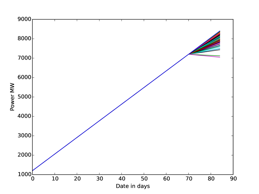
Delta tangent.

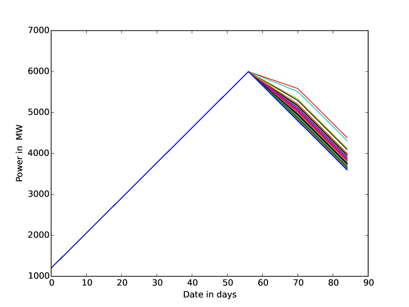
Analytic optimal.

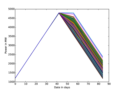
Numerical.

Figure 1: Hedging simulations in MW for finite market depth with $8$ hedging dates and a correlation of -0.4.

5 Numerical convergence of the two algorithms

In this section, we study the influence on the results of the number of mesh and the number of trajectories taken in optimization. To this end, we take the infinite market depth test case with a number of hedging dates equal to $8$. As shown in lemma 4.1, in the continuous case, the conditional variance is quadratic in the future value and is independent of the open position, while the optimal control is only affine with the open position.
As a reference, we take the average of $100$ runs of each algorithm using $12\times 12$ meshes and one million trajectories in optimization. By construction, the local regression algorithm tries to give a partition such that the number of trajectories belonging to a cell is constant. As a rule of the thumb, the number of trajectories on each mesh is kept roughly constant (so here equal to $7000$) while changing the number of mesh used. First, we take a number of mesh as $n\times n$ which is clearly not optimal: the number of mesh in the $F$ and the $D$ direction should be taken different and dependent on the volatilities and mean reverting coefficients. On the table 10, we give the average of $100$ runs obtained with algorithm 1 and 2 for different numbers of meshes. We also plot the standard deviation of the calculation $\hat{\sigma}$ divided by $\sqrt{100}$ as an indicator of the error. The bias due to a small number of mesh is rather small for both algorithms. Off course using a small number of mesh leads to a rather high variance of the result obtained.

Number of meshes	$1\times 1$	$2\times 2$	$4\times 4$	$6\times 6$
Average algo. 1	7.894e+14	7.865e+14	7.876e+14	7.877e+14
$\frac{\hat{\sigma}}{\sqrt{100}}$ algo. 1	1.525e+12	6.812e+11	3.602e+11	2.436e+11
Average algo. 2	7.869e+14	7.847e+14	7.861e+14	7.862e+14
$\frac{\hat{\sigma}}{\sqrt{100}}$ algo. 2	1.524e+12	6.791e+11	3.577e+11	2.445e+11

Number of meshes	$8\times 8$	$10\times 10$	$12\times 12$
Average algo. 1	7.876e+14	7.875e+14	7.875e+14
$\frac{\hat{\sigma}}{\sqrt{100}}$ algo. 1	1.888e+11	1.21038e+11	1.227e+11
Average algo. 2	7.860e+14	7.860e+14	7.860e+14
$\frac{\hat{\sigma}}{\sqrt{100}}$ algo. 2	1.906e+11	1.221e+11	1.242e+11

Table 10: Convergence study of the two algorithms with the number of mesh keeping the same number of trajectories (roughly 7000) on each mesh.

In table 11, we choose to keep a number $8\times 8$ mesh and increase the number of trajectories per mesh.

Number of trajectories	50000	100000	200000	440000	1000000
Average algo. 1	7.8399e+14	7.8643e+14	7.8700e+14	7.8759e+14	7.87729e+14
$\frac{\hat{\sigma}}{\sqrt{100}}$ algo. 1	4.624e+11	3.121e+11	2.621e+11	1.888e+11	1.23053e+11
Average algo. 2	7.7126e+14	7.8007e+14	7.8378e+14	7.86048e+14	7.87052e+14
$\frac{\hat{\sigma}}{\sqrt{100}}$ algo. 2	4.686e+11	3.141e+11	2.664e+11	1.906e+11	1.23911e+11

Table 11: Using $8\times 8$ meshes, convergence study of the two algorithms increasing the number of particles.

Indeed, both algorithm give similar results for a high number of particles per mesh. However, for a low number of particles per mesh, algorithm 1 presents a lower bias than algorithm 2.
At last we want to check that the control is well calculated. In the general case the optimal controls is in dimension three but in the continuous case the formula of lemma 4.1 gives a mono-dimensional representation of the optimal control.
The optimal control has been calculated with algorithm 2 and projected on the local function basis. Then we can reconstruct the optimal position calculated by the algorithm and compare the solution with the formula in lemma 4.1. The figure 2 shows that the numerical optimal control is affine and that even if the variance obtained with 8 hedging dates is very close to the continuous one, the optimal control is still far away from the continuous one. Increasing the number of hedging dates permits to be closer to the continuous optimal control.

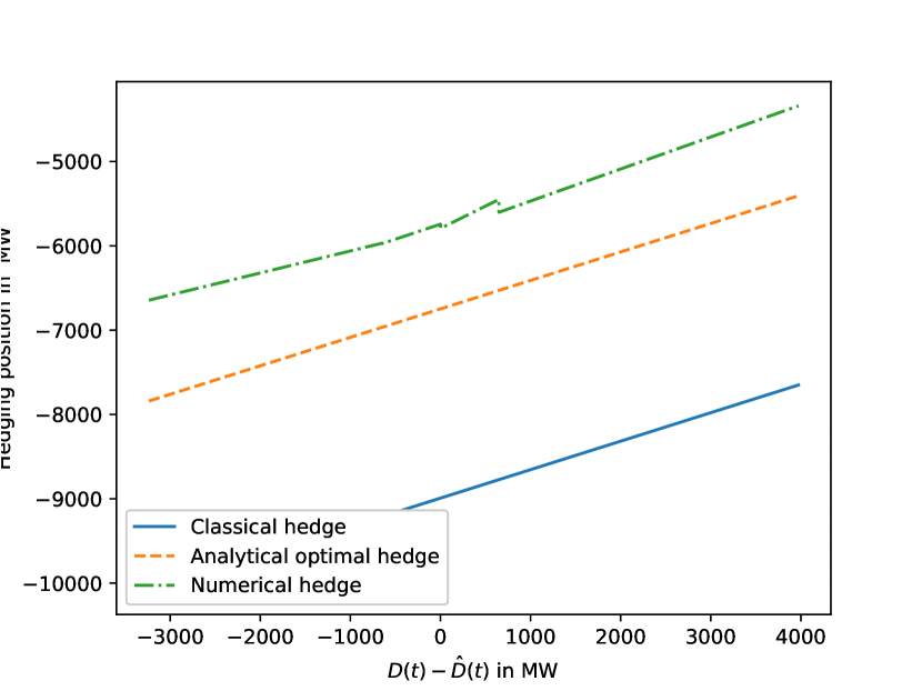
8 hedging dates.

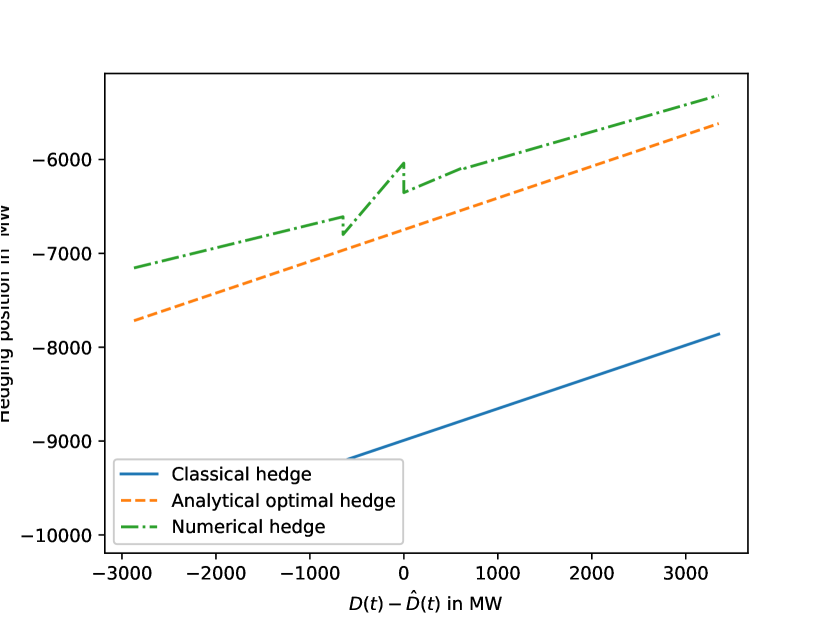
14 hedging dates.

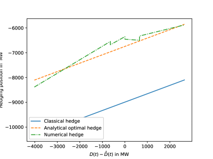
26 hedging dates.

Figure 2: Comparison of numerical optimal position, optimal analytic position, and classical hedge obtained 20 days before delivery for different number of hedging dates using $4$ basis functions for the open position.

6 Conclusion

In the case of mean variance hedging of the wealth portfolio some effective algorithms has been developed to find the optimal strategy taking into account the transaction costs, the limited availability of the hedging products, the fact that hedging is only achieved at discrete dates.
We have shown on a realistic case in energy market that taking in account the reality of the market depth has an important impact on the efficiency of the hedging strategy.
This algorithm could be extended to non symmetric risk measure to take into account the fact that managers wants to favor gains as in gobet2018option.

7 Appendix

We give the proof of lemma 4.1:

The solution of the problem (4.4) is known to be given in the case of martingale assets by the Galtchouk-Kunita-Wananabe decomposition and

$$V(t,D(t),F(t,T))=\mathbb{E}\left[D(T)F(T,T)|{\cal F}_{t}\right],$$

which can be calculated as follows:

$$V(t,D(t),F(t,T))= F(t,T)\left[\hat{D}(T)+(D(t)-\hat{D}(t))e^{-a_{D}(T-t)}+\right.$$

$$\left.\quad\quad\rho\sigma_{E}\sigma_{D}\frac{1-e^{-(a_{E}+a_{D})(T-t)}}{a_{E}+a_{D}}\right].$$

The value function $V$ being a martingale, using Ito lemma we get:

$$D(T)F(T,T)= V(0,D(0),F(0,T))+\int_{0}^{T}\frac{\partial V}{\partial D}(s,D(s),F(s,T))\sigma_{D}dW^{D}_{s}+$$

$$\int_{0}^{T}\frac{\partial V}{\partial F}(s,D(s),F(s,T))\sigma_{E}F(s,T)e^{-a_{E}(T-s)}dW^{E}_{s},$$

so using $W^{D}_{t}=\rho W^{E}_{t}+\sqrt{1-\rho^{2}}\hat{W}^{D}_{t}$ with $\hat{W}^{D}_{t}$ orthogonal to $W^{E}_{t}$ in ${\cal L}^{2}$:

$$D(T)F(t,T)= V(0,D(0),F(0,T))+\int_{0}^{T}\left[\frac{\partial V}{\partial F}(s,D(s),F(s,T))+\right.$$

$$\left.\quad\quad\rho\frac{\sigma_{D}e^{a_{E}(T-s)}}{\sigma_{E}F(s,T)}\frac{\partial V}{\partial D}(s,D(s),F(s,T))\right]dF(s,T)$$

$$+\sqrt{1-\rho^{2}}\frac{\partial V}{\partial D}(s,D(s),F(s,T))\sigma_{D}d\hat{W}^{D}_{s}.$$ (7.1)

The second part in the previous integral represents the non hedgable part of the asset and the optimal hedge is given by:

$$\nu(t,D(t),F(T,T))= \frac{\partial V}{\partial F}(t,D(t),F(t,T))+\rho\frac{\sigma_{D}e^{a_{E}(T-s)}}{\sigma_{E}F(t,T)}\frac{\partial V}{\partial D}(t,D(t),F(t,T)).$$ (7.2)

Introducing the forward tangent process

$$Y_{t}^{T}=e^{-\frac{V(t,T)}{2}+e^{-a_{E}(T-t)}\hat{W}^{E}_{t}},$$

we get

$$\frac{\partial V}{\partial F}(t,D(t),F(t,T))= \mathbb{E}(D(T)Y^{T}_{T}|{\cal F}_{t})/Y_{t}^{T},$$

$$\frac{\partial V}{\partial D}(t,D(t),F(t,T))= e^{-a_{D}(T-t)}F(t,T),$$ (7.3)

so that

$$\frac{\partial V}{\partial F}(t,D(t),F(t,T)) =\hat{D}(T)+(D(t)-\hat{D}(t))e^{-a_{D}(T-t)}+$$

$$\rho\sigma_{E}\sigma_{D}\frac{1-e^{-(a_{E}+a_{D})(T-t)}}{a_{E}+a_{D}}.$$ (7.4)

Plugging equation (7) in equation (7) and equation (7) in equation (7.2) gives the optimal hedging strategy. The residual risk is straightforward.

8 Acknowledgements and Declarations of Interest

Acknowledgements: This work has benefited from the financial support of the ANR Caesars.
Declarations of Interest: The author reports no conflicts of interest. The author alone is responsible for the content and writing of the paper.

References

• Aïd (\APACyear2015) \APACinsertmetastaraid2015electricity{APACrefauthors}Aïd, R.  \APACrefYear2015. \APACrefbtitleElectricity derivatives Electricity derivatives. \APACaddressPublisherSpringer. {APACrefDOI} \doi10.1007/978-3-319-08395-7_2 \PrintBackRefs\CurrentBib
• Bender \BBA Denk (\APACyear2007) \APACinsertmetastarbender2007forward{APACrefauthors}Bender, C.\BCBT \BBA Denk, R.  \APACrefYearMonthDay2007. \BBOQ\APACrefatitleA forward scheme for backward SDEs A forward scheme for backward sdes.\BBCQ \APACjournalVolNumPagesStochastic processes and their applications117121793–1812. {APACrefDOI} \doi10.1016/j.spa.2007.03.005 \PrintBackRefs\CurrentBib
• Bertsimas \BOthers. (\APACyear2000) \APACinsertmetastarbertsimas2000time{APACrefauthors}Bertsimas, D., Kogan, L.\BCBL \BBA Lo, A\BPBIW.  \APACrefYearMonthDay2000. \BBOQ\APACrefatitleWhen is time continuous? When is time continuous?\BBCQ \APACjournalVolNumPagesJournal of Financial Economics552173–204. {APACrefDOI} \doi10.2139/ssrn.116688 \PrintBackRefs\CurrentBib
• Beutner (\APACyear2007) \APACinsertmetastarbeutner2007mean{APACrefauthors}Beutner, E.  \APACrefYearMonthDay2007. \BBOQ\APACrefatitleMean–variance hedging under transaction costs Mean–variance hedging under transaction costs.\BBCQ \APACjournalVolNumPagesMathematical Methods of Operations Research653539–557. {APACrefDOI} \doi10.1007/s00186-006-0134-9 \PrintBackRefs\CurrentBib
• Bouchard \BBA Warin (\APACyear2012) \APACinsertmetastarbouchard2012monte{APACrefauthors}Bouchard, B.\BCBT \BBA Warin, X.  \APACrefYearMonthDay2012. \BBOQ\APACrefatitleMonte-Carlo valuation of American options: facts and new algorithms to improve existing methods Monte-carlo valuation of american options: facts and new algorithms to improve existing methods.\BBCQ \BIn \APACrefbtitleNumerical methods in finance Numerical methods in finance (\BPGS 215–255). \APACaddressPublisherSpringer. {APACrefDOI} \doi10.1007/978-3-642-25746-9_7 \PrintBackRefs\CurrentBib
• Černy (\APACyear2004) \APACinsertmetastarvcerny2004dynamic{APACrefauthors}Černy, A.  \APACrefYearMonthDay2004. \BBOQ\APACrefatitleDynamic programming and mean-variance hedging in discrete time Dynamic programming and mean-variance hedging in discrete time.\BBCQ \APACjournalVolNumPagesApplied Mathematical Finance1111–25. {APACrefDOI} \doi10.1080/1350486042000196164 \PrintBackRefs\CurrentBib
• Denis \BBA Kabanov (\APACyear2010) \APACinsertmetastardenis2010mean{APACrefauthors}Denis, E.\BCBT \BBA Kabanov, Y.  \APACrefYearMonthDay2010. \BBOQ\APACrefatitleMean square error for the Leland–Lott hedging strategy: convex pay-offs Mean square error for the leland–lott hedging strategy: convex pay-offs.\BBCQ \APACjournalVolNumPagesFinance and Stochastics144625–667. {APACrefDOI} \doi10.1007/s00780-010-0130-z \PrintBackRefs\CurrentBib
• Duffie \BBA Richardson (\APACyear1991) \APACinsertmetastarduffie1991mean{APACrefauthors}Duffie, D.\BCBT \BBA Richardson, H\BPBIR.  \APACrefYearMonthDay1991. \BBOQ\APACrefatitleMean-variance hedging in continuous time Mean-variance hedging in continuous time.\BBCQ \APACjournalVolNumPagesThe Annals of Applied Probability1–15. {APACrefDOI} \doi10.1214/aoap/1177005978 \PrintBackRefs\CurrentBib
• Föllmer \BBA Schweizer (\APACyear1988) \APACinsertmetastarfollmer1988hedging{APACrefauthors}Föllmer, H.\BCBT \BBA Schweizer, M.  \APACrefYearMonthDay1988. \BBOQ\APACrefatitleHedging by sequential regression: An introduction to the mathematics of option trading Hedging by sequential regression: An introduction to the mathematics of option trading.\BBCQ \APACjournalVolNumPagesASTIN Bulletin: The Journal of the IAA182147–160. {APACrefDOI} \doi10.2143/ast.18.2.2014948 \PrintBackRefs\CurrentBib
• Gatheral (\APACyear2010) \APACinsertmetastargatheral2010no{APACrefauthors}Gatheral, J.  \APACrefYearMonthDay2010. \BBOQ\APACrefatitleNo-dynamic-arbitrage and market impact No-dynamic-arbitrage and market impact.\BBCQ \APACjournalVolNumPagesQuantitative finance107749–759. {APACrefDOI} \doi10.1080/14697680903373692 \PrintBackRefs\CurrentBib
• Gevret \BOthers. (\APACyear2016) \APACinsertmetastargevret2016stochastic{APACrefauthors}Gevret, H., Lelong, J.\BCBL \BBA Warin, X.  \APACrefYear2016.   \APACrefbtitleSTochastic OPTimization library in C++ Stochastic optimization library in c++ \APACtypeAddressSchool\BUPhD.   \APACaddressSchoolEDF Lab. \PrintBackRefs\CurrentBib
• Gobet \BOthers. (\APACyear2005) \APACinsertmetastargobet2005regression{APACrefauthors}Gobet, E., Lemor, J\BHBIP.\BCBL \BBA Warin, X.  \APACrefYearMonthDay2005. \BBOQ\APACrefatitleA regression-based Monte Carlo method to solve backward stochastic differential equations A regression-based monte carlo method to solve backward stochastic differential equations.\BBCQ \APACjournalVolNumPagesThe Annals of Applied Probability1532172–2202. {APACrefDOI} \doi10.1214/105051605000000412 \PrintBackRefs\CurrentBib
• Gobet \BOthers. (\APACyear2018) \APACinsertmetastargobet2018option{APACrefauthors}Gobet, E., Pimentel, I.\BCBL \BBA Warin, X.  \APACrefYearMonthDay2018. \BBOQ\APACrefatitleOption valuation and hedging using asymmetric risk function: asymptotic optimality through fully nonlinear Partial Differential Equations Option valuation and hedging using asymmetric risk function: asymptotic optimality through fully nonlinear partial differential equations.\BBCQ \APACjournalVolNumPagesHal preprint hal-01761234. \PrintBackRefs\CurrentBib
• Goutte \BOthers. (\APACyear2014) \APACinsertmetastargoutte2014variance{APACrefauthors}Goutte, S., Oudjane, N.\BCBL \BBA Russo, F.  \APACrefYearMonthDay2014. \BBOQ\APACrefatitleVariance optimal hedging for continuous time additive processes and applications Variance optimal hedging for continuous time additive processes and applications.\BBCQ \APACjournalVolNumPagesStochastics An International Journal of Probability and Stochastic Processes861147–185. {APACrefDOI} \doi10.1080/17442508.2013.774402 \PrintBackRefs\CurrentBib
• Hayashi \BBA Mykland (\APACyear2005) \APACinsertmetastarhayashi2005evaluating{APACrefauthors}Hayashi, T.\BCBT \BBA Mykland, P\BPBIA.  \APACrefYearMonthDay2005. \BBOQ\APACrefatitleEvaluating hedging errors: an asymptotic approach Evaluating hedging errors: an asymptotic approach.\BBCQ \APACjournalVolNumPagesMathematical finance152309–343. {APACrefDOI} \doi10.1111/j.0960-1627.2005.00221.x \PrintBackRefs\CurrentBib
• Kabanov \BBA Safarian (\APACyear1997) \APACinsertmetastarkabanov1997leland{APACrefauthors}Kabanov, Y\BPBIM.\BCBT \BBA Safarian, M\BPBIM.  \APACrefYearMonthDay1997. \BBOQ\APACrefatitleOn Leland’s strategy of option pricing with transactions costs On leland’s strategy of option pricing with transactions costs.\BBCQ \APACjournalVolNumPagesFinance and Stochastics13239–250. {APACrefDOI} \doi10.1007/s007800050023 \PrintBackRefs\CurrentBib
• Langrené \BBA Warin (\APACyear2017) \APACinsertmetastarlangrene2017fast{APACrefauthors}Langrené, N.\BCBT \BBA Warin, X.  \APACrefYearMonthDay2017. \BBOQ\APACrefatitleFast and stable multivariate kernel density estimation by fast sum updating Fast and stable multivariate kernel density estimation by fast sum updating.\BBCQ \APACjournalVolNumPagesarXiv preprint arXiv:1712.00993. \PrintBackRefs\CurrentBib
• Leland (\APACyear1985) \APACinsertmetastarleland1985option{APACrefauthors}Leland, H\BPBIE.  \APACrefYearMonthDay1985. \BBOQ\APACrefatitleOption pricing and replication with transactions costs Option pricing and replication with transactions costs.\BBCQ \APACjournalVolNumPagesThe journal of finance4051283–1301. {APACrefDOI} \doi10.1111/j.1540-6261.1985.tb02383.x \PrintBackRefs\CurrentBib
• Longstaff \BBA Schwartz (\APACyear2001) \APACinsertmetastarlongstaff2001valuing{APACrefauthors}Longstaff, F\BPBIA.\BCBT \BBA Schwartz, E\BPBIS.  \APACrefYearMonthDay2001. \BBOQ\APACrefatitleValuing American options by simulation: a simple least-squares approach Valuing american options by simulation: a simple least-squares approach.\BBCQ \APACjournalVolNumPagesThe review of financial studies141113–147. {APACrefDOI} \doi10.1093/rfs/14.1.113 \PrintBackRefs\CurrentBib
• Ludkovski \BBA Maheshwari (\APACyear2018) \APACinsertmetastarludkovski2018simulation{APACrefauthors}Ludkovski, M.\BCBT \BBA Maheshwari, A.  \APACrefYearMonthDay2018. \BBOQ\APACrefatitleSimulation Methods for Stochastic Storage Problems: A Statistical Learning Perspective Simulation methods for stochastic storage problems: A statistical learning perspective.\BBCQ \APACjournalVolNumPagesarXiv preprint arXiv:1803.11309. \PrintBackRefs\CurrentBib
• Motoczyński (\APACyear2000) \APACinsertmetastarmotoczynski2000multidimensional{APACrefauthors}Motoczyński, M.  \APACrefYearMonthDay2000. \BBOQ\APACrefatitleMultidimensional Variance-Optimal Hedging in Discrete-Time Model - A General Approach Multidimensional variance-optimal hedging in discrete-time model - a general approach.\BBCQ \APACjournalVolNumPagesMathematical Finance102243–257. {APACrefDOI} \doi10.1111/1467-9965.00092 \PrintBackRefs\CurrentBib
• Pergamenshchikov (\APACyear2003) \APACinsertmetastarpergamenshchikov2003limit{APACrefauthors}Pergamenshchikov, S.  \APACrefYearMonthDay2003. \BBOQ\APACrefatitleLimit theorem for Leland’s strategy Limit theorem for leland’s strategy.\BBCQ \APACjournalVolNumPagesThe Annals of Applied Probability1331099–1118. {APACrefDOI} \doi10.1214/aoap/106020283 \PrintBackRefs\CurrentBib
• Schweizer (\APACyear1995) \APACinsertmetastarschweizer1995variance{APACrefauthors}Schweizer, M.  \APACrefYearMonthDay1995. \BBOQ\APACrefatitleVariance-optimal hedging in discrete time Variance-optimal hedging in discrete time.\BBCQ \APACjournalVolNumPagesMathematics of Operations Research2011–32. {APACrefDOI} \doi10.1287/moor.20.1.1 \PrintBackRefs\CurrentBib
• Schweizer (\APACyear1999) \APACinsertmetastarschweizer1999guided{APACrefauthors}Schweizer, M.  \APACrefYearMonthDay1999. \APACrefbtitleA guided tour through quadratic hedging approaches A guided tour through quadratic hedging approaches \APACbVolEdTR\BTR. \APACaddressInstitutionDiscussion Papers, Interdisciplinary Research Project 373: Quantification and Simulation of Economic Processes. {APACrefDOI} \doi10.1017/cbo9780511569708.016 \PrintBackRefs\CurrentBib
• Soner \BOthers. (\APACyear1995) \APACinsertmetastarsoner1995there{APACrefauthors}Soner, H\BPBIM., Shreve, S\BPBIE.\BCBL \BBA Cvitanić, J.  \APACrefYearMonthDay1995. \BBOQ\APACrefatitleThere is no nontrivial hedging portfolio for option pricing with transaction costs There is no nontrivial hedging portfolio for option pricing with transaction costs.\BBCQ \APACjournalVolNumPagesThe Annals of Applied Probability327–355. {APACrefDOI} \doi10.1214/aoap/1177004767 \PrintBackRefs\CurrentBib
• Tankov \BBA Voltchkova (\APACyear2009) \APACinsertmetastartankov2009asymptotic{APACrefauthors}Tankov, P.\BCBT \BBA Voltchkova, E.  \APACrefYearMonthDay2009. \BBOQ\APACrefatitleAsymptotic analysis of hedging errors in models with jumps Asymptotic analysis of hedging errors in models with jumps.\BBCQ \APACjournalVolNumPagesStochastic processes and their applications11962004–2027. {APACrefDOI} \doi10.1016/j.spa.2008.10.002 \PrintBackRefs\CurrentBib
• Warin (\APACyear2012) \APACinsertmetastarwarin2012gas{APACrefauthors}Warin, X.  \APACrefYearMonthDay2012. \BBOQ\APACrefatitleGas storage hedging Gas storage hedging.\BBCQ \BIn \APACrefbtitleNumerical Methods in Finance Numerical methods in finance (\BPGS 421–445). \APACaddressPublisherSpringer. {APACrefDOI} \doi10.1007/978-3-642-25746-9_14 \PrintBackRefs\CurrentBib
• Zhang (\APACyear1999) \APACinsertmetastarzhang1999couverture{APACrefauthors}Zhang, R.  \APACrefYear1999.   \APACrefbtitleCouverture approchée des options Européennes Couverture approchée des options européennes \APACtypeAddressSchool\BUPhD.   \APACaddressSchoolEcole des Ponts ParisTech. \PrintBackRefs\CurrentBib