A multiple scales approach to maximal superintegrability

Abstract

In this paper we present a simple, algorithmic test to establish if a Hamiltonian system is maximally superintegrable or not. This test is based on a very simple corollary of a theorem due to Nekhoroshev and on a perturbative technique called multiple scales method. If the outcome is positive, this test can be used to suggest maximal superintegrability, whereas when the outcome is negative it can be used to disprove it. This method can be regarded as a finite dimensional analog of the multiple scales method as a way to produce soliton equations. We use this technique to show that the real counterpart of a mechanical system found by Jules Drach in 1935 is, in general, not maximally superintegrable. We give some hints on how this approach could be applied to classify maximally superintegrable systems by presenting a direct proof of the well-known Bertrand’s theorem.

1 Introduction

The notion of integrability in Classical Mechanics is well established since the times of Liouville [49] and, roughly speaking, means the existence of a “sufficiently” high number of integrals of motion. To be more precise assume we are given a Hamiltonian system with Hamiltonian $H=H\left(\mathbf{p},\mathbf{q}\right)$ with $n$ degrees of freedom, i.e. $\mathbf{q}=\left(q_{1},\dots,q_{n}\right)$ and $\mathbf{p}=\left(p_{1},\dots,p_{n}\right)$. We say that the mechanical system defined by the Hamiltonian $H$ is integrable if there exist $n$ integrals of motion, i.e. $n$ functions $H_{i}$ $i=1,\dots,n$ which Poisson-commute with the Hamiltonian:

$$\left\{H_{i},H\right\}=0.$$ (1)

If an integral of motion is polynomial in $\mathbf{p}$, then its total degree as polynomial in $\mathbf{p}$ is called the order of the integral of motion. The Hamiltonian, which trivially commutes with itself, is included in the list as $H_{1}=H$. These integrals of motion must be well defined functions on the phase space, i.e. analytic and single-valued. Moreover, they have to be in involution:

$$\left\{H_{i},H_{j}\right\}=0,\quad i,j\in\{1,\dots,n\}.$$ (2)

Finally, they must be functionally independent:

$$\rank\frac{\partial(H_{1},\dots,H_{n})}{\partial(\mathbf{p},\mathbf{q})}=n.$$ (3)

Indeed, the knowledge of these kinds of integrals permits the integration of the equations of motion associated to $H$. This is the content of the famous Liouville theorem [49, 82]. We remark that the application of Liouville’s theorem yields other $n-1$ quantities that are Poisson-commuting with the Hamiltonian. Usually, these quantities are not integrals of motion in the sense of our definition since they are not well defined functions on the phase space. Integrability in Classical Mechanics implies that the motion is constrained on a subspace of the full phase space. With some additional assumptions on the geometric structure of the integrals of motion, it is possible to prove that the motion is quasi-periodic on some tori in the phase space [4, 5].

When there exist more than $n$, say $n+k$ with $1\leq k\leq n-1$, independent integrals of motion, we say that the system is superintegrable. When $k=1$ the system is minimally superintegrable, whereas when $k=n-1$ it is maximally superintegrable. In the case $n=2$ the two notions coincide. The search for superintegrable systems started more than a half century ago with the seminal paper [27], but the name “superintegrability” has been introduced only in [72] about the Calogero-Moser system [11, 13, 52]. However, we remark that the definition of superintegrability introduced in [72] is in fact the definition of maximal superintegrability given above. For a full historical and a state-of-art perspective on superintegrability we refer to the review [51] and references therein.

From the algebraic point of view the structure of superintegrable systems is richer than that of integrable systems because the additional integrals will not be in involution with the previous ones. This gives rise to many interesting non-abelian algebraic structures. Usually, they are finitely generated polynomial algebras, only exceptionally finite dimensional Lie algebras or Kac-Moody algebras [20]. For this reason superintegrability is also often called non-abelian integrability. From the geometrical point of view superintegrability restricts trajectories to an $n-k$ dimensional subspace of the phase space. This implies that the following Theorem holds true:

Theorem 1 (Nekhoroshev [55]).

Let us consider an Hamiltonian system with Hamiltonian $H=H\left(\mathbf{p},\mathbf{q}\right)$. If such system is maximally superintegrable then every bounded orbit is closed and periodic.

Intuitively this happens because in the maximally superintegrable case the trajectories are restricted to one-dimensional subspace of the phase space. Therefore, any bounded orbit is just diffeomorphic to a circle. Of course Theorem 1 has an immediate corollary given by:

Corollary 2.

If a Hamiltonian system with Hamiltonian $H=H\left(\mathbf{p},\mathbf{q}\right)$ possesses at least one bounded orbit which is neither closed nor periodic, then it is not maximally superintegrable.

In this paper we suggest a simple, algorithmic, perturbative test based on Corollary 2 which allows to prove if a system is maximally superintegrable or not. This test can be particularly useful when $n=2$ since, as noted above, in this case the notion of superintegrability and maximal superintegrability coincide.

The paper is structured as follows. In Section 2 we describe our method for disproving or suggesting maximal superintegrability. We give a concise introduction to the multiple scales method [45, 18]: a perturbative technique aimed to avoid resonant, i.e. diverging, terms in the asymptotic expansion and to describe physical phenomena happening on different time scales. In Section 3 we present some relevant examples of application of the method. In particular we discuss the field of applicability of the method and we confront it with other techniques. We present the known example of the Tremblay-Turbiner-Winternitz (TTW) system [78], where the method of Section 2 suggests (maximal) superintegrability. We also present a new result about the Drach system [22]. Using the method presented in Section 2 we show that the Drach system is, in general, not superintegrable. Finally, we show how it is possible to use such a method to classify maximally superintegrable systems giving an alternative proof of the famous Bertrand’s Theorem [7]. In Section 4 we give some conclusions and perspectives for further developments. We comment on the analogy between our method, which has been applied to finite dimensional systems, and the ones used in the infinite dimensional framework as a way to produce soliton equations [84, 15, 16, 12].

2 The method

Our approach in disproving or suggesting maximal superintegrability is based on Corollary 2 and on the so-called multiple scales method. The multiple scales analysis is a perturbation technique whose history dates back to the 18th century. The bases for the multiple scales method were laid in the works by Lindstedt [48] and Poincaré [66], it was developed in its modern form in [45, 18]. The core of this approach is to find asymptotic approximated solutions of a system of differential equations when the standard perturbation theory produces secular terms. During the years, the multiple scales analysis has proved to be very useful in the construction of approximate solutions of differential equations, and is now included in every textbook on perturbation theory [54, 6, 44, 39]. Such a powerful method has also found applications in fields which do not seem to be correlated with such problems, for example in the theory of integrable systems in infinite dimensions [84, 15, 16, 12].

The key feature that allows the elimination of the secular terms is the introduction of fast-scale variables and slow-scales variables in a way that the dependence on the slow-scale variables will prevent the secularities. To be more precise, suppose that we are given a system of second-order ordinary differential equations with independent variable $t$ and dependent variables $\mathbf{x}\left(t\right)=\left(x_{1}\left(t\right),\dots,x_{n}\left(t\right)\right)$:

$$\mathbf{\ddot{x}}=\mathbf{F}_{\varepsilon}\left(\mathbf{x},\mathbf{\dot{x}}\right),$$ (4)

where the $\varepsilon$ subscript means that we have dependence on a “small” parameter $\varepsilon$, i.e. $\varepsilon\to 0^{+}$. From now on this condition on the parameter $\varepsilon$ will be always assumed. We suppose that $\mathbf{x}$ has an asymptotic expansion of the form:

$$\mathbf{x}\left(t\right)=\sum_{i=0}^{N+M}\varepsilon^{i}\mathbf{x}^{(i)}\left(t_{0},t_{1},t_{2},\dots,t_{N}\right)+\mathcal{O}\left(\varepsilon^{N+M+1}\right),$$ (5)

truncated at some positive integer $N+M$, with $M\geq 0$. In the right hand side of (5) the dependence on the time variable $t$ appears through the so-called scales ${t_{i}=t_{i}(t,\varepsilon)}$. Intuitively, the scales isolate different behaviors inside equation (4). E.g. in the damped harmonic oscillator the oscillations and the amplitude suppression are phenomena happening on different time scales. The number of scales to be introduced depends on the desired asymptotic approximation order: the expansion is guaranteed to be asymptotic until

$$t_{N}\left(t,\varepsilon\right)=\mathcal{O}\left(1\right)$$ (6)

is satisfied. The number of scales also sets the approximation error, in the sense that the maximum discrepancy from the complete solution

$$\max_{t\in\left[0,t_{max}\right]}\absolutevalue{\mathbf{x}(t)-\sum_{i=0}^{N+M-1}\varepsilon^{i}\mathbf{x}^{(i)}\left(t_{0},t_{1},t_{2},\dots,t_{N}\right)}$$ (7)

is $\mathcal{O}\left(\varepsilon^{N+M}\right)$, where $t_{max}$ is the time such that the condition (6) holds.

The mathematical structure of the scales is the most delicate point in the whole expansion method: it involves the knowledge of the structure of the system (4), and the constraint that they must be non-decreasing functions of $t$ satisfying the condition:

$$\lim_{\varepsilon\to 0^{+}}\dfrac{t_{i+1}(t,\varepsilon)}{t_{i}(t,\varepsilon)}=0,\quad\forall\,i=0,1,\dots,N-1.$$ (8)

Condition (8) just states that the scales are well-ordered, i.e. phenomena happening at the scale $t_{i+1}$ are slower than those happening on scale $t_{i}$. In many cases, and in our paper we will do so, one can just consider the so-called trivial time scales:

$$t_{i}=\varepsilon^{i}t,$$ (9)

which are non-decreasing linear functions of $t$ and satisfy the condition (8). We note that in general $N$ has to be sufficiently high not just to give a longer asymptotic range of validity of the expansion, but also to capture the behavior of the system.

The substitution (5) can be extended to all the derivatives of $\mathbf{x}$ by differentiation or, more operatively, by substituting

$$\frac{\mathrm{d}}{\mathrm{d}t}=\sum_{i=0}^{N}\frac{\partial t_{i}}{\partial t}\frac{\partial}{\partial t_{i}},$$ (10)

which in the case of the trivial time scales is particularly simple:

$$\frac{\mathrm{d}}{\mathrm{d}t}=\sum_{i=0}^{N}\varepsilon^{i}\frac{\partial}{\partial t_{i}}.$$ (11)

Substituting the series (5) and all its derivatives in equation (4) using (10), and eventually expanding in Taylor series with respect to $\varepsilon$, we obtain a polynomial in $\varepsilon$ which must be identically equal to zero. We can then separately set to zero all the coefficients of $\varepsilon$-powers and obtain a system of $N+M+1$ partial differential equations. If the scales are correctly chosen, the $\varepsilon^{0}$-equation will contain $\mathbf{x}^{(0)}$ only and will depend just on $t_{0}$. This will give rise to a solution depending on arbitrary functions of the remaining scales $t_{1},\dots,t_{N}$. Substituting $\mathbf{x}^{(0)}$ into the $\varepsilon^{1}$-equation we use these arbitrary functions to prevent the birth of the secular terms in $\mathbf{x}^{(1)}$. Solving iteratively for the remaining $\mathbf{x}^{(i)}$ one finally writes down the $N+M$ terms of the desired expansion (5). In the case of high order expansions ($N>1$) sometimes the previous iterative method is not sufficient to completely specify the terms of the asymptotic series. In these cases the strategy of the suppression of the order mixing is adopted: it consists in eliminating from the $\varepsilon^{i+1}$-equation all the contributions coming from the arbitrary functions arising from lower orders solutions $\mathbf{x}^{(i)}$, $\mathbf{x}^{(i-1)}$, etc. This increases the accuracy of the first $i$ terms by reducing the amount of corrective terms in $\mathbf{x}^{(i+1)}$ [39].

Remark 1.

Unlike the usual pertubation theory where the object seeked is of increasing precision in $\varepsilon$, the aim of the multiple scales method is to derive an object of “minimal” precision, but valid for a longer time scale, i.e. a true asymptotic expansion. If one sets in (5) $M=0$, as it is usually done, then the output of the method is an $\varepsilon$-precision approximate solution of the form:

$$\mathbf{x}=\mathbf{x}^{(0)}\left(t_{0},t_{1},\dots,t_{N}\right)+\mathcal{O}\left(\varepsilon\right),$$ (12)

valid until $t_{N}=\mathcal{O}\left(1\right)$.

In order to disprove or suggest the maximal superintegrability of a Hamiltonian system we will need several steps. Indeed, if we want to apply the multiple scales method, we will need to introduce into our Hamilton’s equations a small parameter $\varepsilon$ which is not, in general, naturally present. To this end we will use a perturbative approach to equilibrium. Moreover, we will need the following technical result:

Lemma 3.

Let us suppose that we are given a system of second-order differential equations in the form (4), such that the dependence on the parameter $\varepsilon$ is analytic in a neighbourhood of $\varepsilon=0$. Assume that every bounded solution of (4) is periodic. Then every bounded perturbative series, analytic in a neighbourhood of $\varepsilon=0$, is periodic at any order.

Proof.

Let us assume we have a bounded analytic perturbative series

$$\mathbf{x}_{P}(t)=\sum_{k=0}^{\infty}\varepsilon^{k}\mathbf{x}^{(k)}(t).$$ (13)

Since $\mathbf{x}_{P}$ is bounded, then it is periodic by assumption. This means that there exists a $T$ such that $\mathbf{x}\left(t+T\right)=\mathbf{x}\left(t\right)$ for every $t\in\mathbb{R}$. Substituting this condition in (13), since the series is analytic in $\varepsilon$, we obtain:

$$\mathbf{x}^{(k)}\left(t+T\right)=\mathbf{x}^{(k)}\left(t\right),\quad\forall k\in\mathbb{N},$$ (14)

which implies that every order of the perturbative series is periodic. Moreover, since we assumed that the system (4) is analytic in a neighbourhood of $\varepsilon=0$ we have that, at every order, the coefficients $\mathbf{x}^{(k)}$ will be approximate solutions of the differential system for $\varepsilon\to 0^{+}$. ∎

Remark 2.

An asymptotic series which is bounded at every power of $\varepsilon$ by a constant $B_{k}$, independent of $\varepsilon$, will satisfy the hypothesis of Lemma 3 provided that the sequence $B_{k}$ is well behaved. Indeed, if for every $k\in\mathbb{N}$ the estimate $\absolutevalue{\mathbf{x}^{\left(k\right)}}\leq B_{k}$, we have from (13):

$$\absolutevalue{\mathbf{x}_{P}}\leq\sum_{k=0}^{\infty}\varepsilon^{k}B_{k}.$$ (15)

The latter series is convergent, by the Cauchy-Hadamard theorem [83], if

$$R^{-1}=\limsup_{k\to\infty}|B_{k}|^{1/k}<\infty.$$ (16)

We remark that in a general multiple-scales expansion the condition of boundness is satisfied at every power of $\varepsilon$. In general, proving explicitly the condition (16) can be quite complicated. However, if the original equation is analytic in a neighbourhood of $\varepsilon=0$, we can assume that (except for some pathological case) such condition is satisfied.

Then, the method we propose can be summarized in the following steps:

1. We put the mechanical system under consideration in Lagrangian form, $L=L\left(\mathbf{q},\mathbf{\dot{q}}\right)$ with $\mathbf{q}=\left(q_{1},\dots,q_{n}\right)\in\mathcal{U}\subset\mathbb{R}^{n}$ and $\dot{\mathbf{q}}=\left(\dot{q}_{1},\dots,\dot{q}_{n}\right)\in T_{\mathbf{q}}\mathcal{U}$, where $\mathcal{U}$ is an open subset of $\mathbb{R}^{n}$. We remark that in general, the generalized coodinates $\mathbf{q}$ may belong to a Riemannian manifold $\mathcal{M}$ of dimension $n$. However, our analysis is local therefore we can always think to be in the appropriate chart. In the cases we will treat in this paper we will deal with natural Lagrangians, i.e. Lagrangians of the form:

   $$L=\frac{1}{2}\left(\mathbf{\dot{q}},A\left(\mathbf{q}\right)\mathbf{\dot{q}}\right)-V\left(\mathbf{q}\right)$$ (17)

   where $A\left(\mathbf{q}\right)=[A_{ij}(\mathbf{q})]$ is a symmetric, positive definite $n\times n$ matrix, with $(\,,\,)$ we denoted the standard scalar product and $V\left(\mathbf{q}\right)$ is the potential. We prefer the Lagragian form over the Hamitonian one of the equations of motion because identifying and isolating resonances for second-order differential equations is easier. The coordinates $\mathbf{q}$ are preferably unbounded. The use of unbounded coordinates, e.g. Cartesian, elliptical and parabolic, is preferred since it is easier to keep track of the secular terms. However, the method can be applied with the required care even when some bounded coordinates are present, see Subsection 3.5.

2. Search for equilibrium positions as stationary points of the potential $V$ i.e. as the points such that $\nabla_{\mathbf{q}}V={\mathbf{0}}$, where $\nabla_{\mathbf{q}}$ denotes the gradient with respect to the $\mathbf{q}$ coordinates. This will give a collection of points to test, say:

   $$\Set{\mathbf{q}_{1},\mathbf{q}_{2}\dots,\mathbf{q}_{m}},\quad m\in\mathbb{N}^{*}.$$ (18)

   In principle the method cannot be applied if no stationary point exists. However, in some cases, it is still possible to apply it. For a discussion of this extension see Subsection 3.5.

3. Determine the linearized equations perturbatively using the expansion:

   $$\mathbf{q}=\mathbf{q}_{l}+\varepsilon\mathbf{Q},\quad l=1,\dots,m.$$ (19)

   In this way we introduce the needed small parameter $\varepsilon$. This analysis is equivalent to the classical one [10, 5], simply the condition $\varepsilon\to 0^{+}$ replaces the “small-norm” requirement usually adopted. The small parameter is used to linearize the equation. In the case of natural Lagrangians (17) the Euler-Lagrange equations are given by [46]:

   $$\sum_{j=1}^{n}A_{kj}\left(\mathbf{q}\right)\ddot{q}_{j}+\sum_{i,j=1}^{n}\Gamma_{ijk}\left(\mathbf{q}\right)\dot{q}_{i}\dot{q}_{j}+\frac{\partial V\left(\mathbf{q}\right)}{\partial q_{k}}=0,\quad k=1,\dots,n,$$ (20)

   where

   $$\Gamma_{ijk}\left(\mathbf{q}\right)\doteq\frac{1}{2}\left(\frac{\partial A_{ik}(\mathbf{q})}{\partial q_{j}}+\frac{\partial A_{jk}(\mathbf{q})}{\partial q_{i}}-\frac{\partial A_{ij}(\mathbf{q})}{\partial q_{k}}\right)$$ (21)

   are the contracted Christoffel symbols [23]. Inserting (19) in the Euler-Lagrange equations (20) we obtain:

   $$\varepsilon\sum_{j=1}^{n}A_{kj}\left(\mathbf{q}_{l}+\varepsilon\mathbf{Q}\right)\ddot{Q}_{j}+\varepsilon^{2}\sum_{i,j=1}^{n}\Gamma_{ijk}\left(\mathbf{q}_{l}+\varepsilon\mathbf{Q}\right)\dot{Q}_{i}\dot{Q}_{j}+\frac{\partial V\left(\mathbf{q}_{l}+\varepsilon\mathbf{Q}\right)}{\partial q_{k}}=0,\quad k=1,\dots,n.$$ (22)

   Expanding the system (22) in Taylor series with respect to $\varepsilon$, since $\mathbf{q}_{l}$ is a stationary point, we get:

   $$\varepsilon\sum_{j=1}^{n}\left[A_{kj}\left(\mathbf{q}_{l}\right)\ddot{Q}_{j}+\frac{\partial^{2}V}{\partial q_{k}\,\partial q_{j}}\left(\mathbf{q}_{l}\right)Q_{j}\right]+\mathcal{O}\left(\varepsilon^{2}\right)=0,\quad k=1,\dots,n.$$ (23)

   Equation (23) can be easily written in vector form as

   $$\varepsilon\left[A\left(\mathbf{q}_{l}\right)\mathbf{\ddot{Q}}+\mathrm{H}\left(V\right)\left(\mathbf{q}_{l}\right)\mathbf{Q}\right]+\mathcal{O}\left(\varepsilon^{2}\right)=\mathbf{0},$$ (24)

   denoting with $\mathrm{H}\left(V\right)\left(\mathbf{q}_{l}\right)$ the Hessian matrix of $V$ evaluated in $\mathbf{q}_{l}$. We just obtained through this perturbative approach the usual linearized Euler-Lagrange equations [5].

4. Given the linearized equations (24), it is well known that their integration can be reduced to a problem in linear algebra which consists in finding the eigenvalues of the symmetric matrix $\mathrm{H}\left(V\right)\left(\mathbf{q}_{l}\right)$ with respect to the scalar product induced by the symmetric and positive definite matrix $A\left(\mathbf{q}_{l}\right)$. Practically, this can be done solving the characteristic equation:

   $$\det\left[\mathrm{H}\left(V\right)\left(\mathbf{q}_{l}\right)-\omega^{2}A\left(\mathbf{q}_{l}\right)\right]=0,$$ (25)

   with respect to $\omega$. The solution of equation (25) yields $n$ solutions for $\omega^{2}$. If every possible value of $\omega^{2}$ is positive, then we say that the equilibrium point is stable. If all the possible values of $\omega^{2}$ are non-negative, then we say that the equilibrium point is neutral. If at least one of the possible values of $\omega^{2}$ is negative, we say that the equilibrium is unstable. As we will discuss, stable equilibrium points give rise to bounded orbits, and this is the reason why we will be interested in this kind of stationary points. We will assume that in the set of points (18) there exists at least one stable point, otherwise the algorithm is not applicable. Therefore, we will continue our discussion assuming that all the possible values of $\omega^{2}$ are positive. Then, we can define the vector $\boldsymbol{\omega}=\left(\omega_{1},\dots,\omega_{n}\right)$ of the $n$ positive, possibly equal, solutions of (25). We call the constants $\omega_{i}$ the fundamental frequencies. Physically, this procedure amounts to make the ansatz:

   $$\mathbf{Q}=\mathbf{S}\cos\left(\omega t+\varphi\right),$$ (26)

   which inserted in (24) is solution if and only if (25) is satisfied. Since the matrices $\mathrm{H}\left(V\right)\left(\mathbf{q}_{l}\right)$ and $A\left(\mathbf{q}_{l}\right)$ are symmetric, to the $n$ fundamental frequencies correspond $n$ independent orthogonal eigenvectors $\mathbf{S}^{(1)},\dots,\mathbf{S}^{(n)}$, i.e. the solutions of:

   $$\left[\mathrm{H}\left(V\right)\left(\mathbf{q}_{l}\right)-\omega^{2}_{i}A\left(\mathbf{q}_{l}\right)\right]\mathbf{S}^{(i)}=\mathbf{0}.$$ (27)

   The general solution of the linearized Euler-Lagrange equation is then given by:

   $$\mathbf{Q}=\sum_{i=1}^{n}\mathbf{S}^{(i)}N_{i}\left(t\right),$$ (28)

   where:

   $$N_{i}(t)=R_{i}\cos\left(\omega_{i}t+\varphi_{i}\right)\,,\quad i=1,\dots,n,$$ (29)

   with $R_{i}$ and $\varphi_{i}$ constants. Then, performing the linear transformation $\mathbf{Q}=S\mathbf{N}$ with $S$ given by:

   $$S=\left[\mathbf{S}^{(1)},\dots,\mathbf{S}^{(n)}\right],$$ (30)

   we have that the system (24) reduces to

   $$\mathbf{\ddot{N}}+\Lambda_{S}\mathbf{N}=\mathbf{0},\quad\Lambda_{S}=S^{T}A\left(\mathbf{q}_{l}\right)^{-1}\mathrm{H}\left(V\right)\left(\mathbf{q}_{l}\right)S=\operatorname{diag}\left(\omega_{1}^{2},\dots,\omega_{n}^{2}\right).$$ (31)

   Thus, in the coordinates $\mathbf{N}$, the system acts as $n$ one-dimensional systems whose solution is given by (29). The coordinates $\mathbf{N}$ are called the normal coordinates. This means that the solution of the system at order $\varepsilon$ is bounded. We introduce the frequencies ratio matrix:

   $$\Delta^{(0)}\left(\mathbf{q}_{l}\right)\doteq\left[\frac{\omega_{i}^{(0)}}{\omega_{j}^{(0)}}\right]_{i,j=1,\dots,n}.$$ (32)

   If the entries of the matrix $\Delta^{(0)}\left(\mathbf{q}_{l}\right)$ (32) are rational then we have found an approximate bounded periodic closed orbit. This implies that the system under scrutiny can be maximally superintegrable. If there exists at least a stable equilibrium point $\mathbf{q}_{l^{*}}$, such that the matrix $\Delta^{(0)}\left(\mathbf{q}_{l^{*}}\right)$ (32) possesses at least an irrational entry then, as a consequence of Corollary 2 and Lemma 3, the system cannot be maximally superintegrable. In the latter case the algorithm terminates here with a negative answer.

5. If all the stable equilibrium points in (18) give rise to closed periodic orbits, we have to check if this conditions is preserved on longer time scales. To this end we return to the Euler-Lagrange equations, say of the form of (20), but we now assume that $\mathbf{Q}=S\mathbf{N}$ where $\mathbf{N}$ is given by a multiple-scale expansion:

   $$\mathbf{N}=\sum_{i=0}^{N+M}\varepsilon^{i}\mathbf{N}^{(i)}\left(t_{0},t_{1},t_{2},\dots,t_{N}\right)+\mathcal{O}\left(\varepsilon^{N+M+1}\right),$$ (33)

   where as time scales we use the trivial ones (9). This asymptotic expansion will give rise to higher order corrections to the fundamental frequencies $\boldsymbol{\omega}$:

   $$\Omega_{j}^{(N)}=\sum_{i=0}^{N}\varepsilon^{i}\omega_{j}^{(i)},\quad j=1,\dots,n.$$ (34)

   We introduce the higher order frequencies ratio matrix:

   $$\Delta^{(N)}\left(\mathbf{q}_{l}\right)\doteq\left[\frac{\Omega_{i}^{(N)}}{\Omega_{j}^{(N)}}\right]_{i,j=1,\dots,n}.$$ (35)

   Again, if the entries of the matrix $\Delta^{(N)}\left(\mathbf{q}_{l}\right)$ are rational, we have found an approximate bounded periodic closed orbit of order $N$. This can suggest maximal superintegrability. If on the contrary we are able to prove that there exists at least a point $\mathbf{q}_{l^{*}}$ and an integer $N^{*}>1$, such that one of the entries of the matrix $\Delta^{(N^{*})}\left(\mathbf{q}_{l^{*}}\right)$ (35) is not rational then, from Corollary 2 and Lemma 3, we can conclude that the system is not maximally superintegrable.

Remark 3.

We observe that in the plane case, i.e. when $n=2$, it is not necessary to consider the “full” matrices (32) and (35), but only the ratios

$$\Delta^{(0)}\left(\mathbf{q}_{l}\right)=\frac{\omega_{1}^{(0)}}{\omega_{2}^{(0)}}\quad\text{and}\quad\Delta^{(N)}\left(\mathbf{q}_{l}\right)=\frac{\Omega_{1}^{(N)}}{\Omega_{2}^{(N)}}$$ (36)

will be relevant.

Remark 4.

At the present stage, in order to show that a system is not maximally superintegrable, it was sufficient to take an expansion (33) such that $N=2$ and $M=0$. It is not known if there exist non-maximally superintegrable systems requiring higher order expansions.

In the next Section we present some examples of the application of the method we just outlined.

3 Examples of application of the method

In this Section we present the practical application of the method we explained in Section 2. In particular we provide five examples which are aimed to underline the importance and the possibilities of the presented procedure.

In Subsections 3.1 and 3.2 we present two simple examples, namely the generalized Hénon-Heiles system [32, 26] and the anisotropic caged oscillator [25]. We use these two examples to discuss the range of the results which can be obtained in the framework of our method, and to confront them with other algorithmic procedures aimed to find integrable systems. In Subsection 3.3 we show that the superintegrability of the Tremblay-Turbiner-Winternitz (TTW) system [78], can be inferred using the algorithm of Section 2. In Subsection 3.4 we present a new result about the so-called Drach system [22]. Applying the method presented in Section 2 we show that the Drach system is not, for general values of the parameters, superintegrable. This result answers a comment made by the authors of [67] where a particular case of this model, which we will call the Drach-Post-Winternitz (DPW) system, was considered and it was shown to be superintegrable. Finally, in Subsection 3.5, we show that the method of Section 2 can be applied as a sieve test for (maximally) superintegrable systems. Indeed, we prove in this framework Bertrand’s theorem [7], which characterizes all the possible central potentials in the plane with bounded and closed orbits.

3.1 The generalized Hénon-Heiles system

As a first application of the method we discuss the so-called generalized Hénon-Heiles Hamiltonian:

$$H_{\text{HH}}=\frac{1}{2}\left(p_{1}^{2}+p_{2}^{2}\right)+\frac{\omega_{1}^{2}}{2}q_{1}^{2}+\frac{\omega_{2}^{2}}{2}q_{2}^{2}+\alpha\left(q_{1}^{2}q_{2}+\beta q_{2}^{3}\right),$$ (37)

where $\omega_{1}$, $\omega_{2}\in\mathbb{R}^{+}$ and $\alpha$, $\beta$ are real parameters. This system is called generalized Hénon-Heiles since it is a generalization of the Hénon-Heiles system which arises for $\omega_{1}=\omega_{2}=1$ and $\beta=-1/3$. The Hénon-Heiles system was introduced in [32] to model the dynamics of a Newtonian axially-symmetric galactic system and it is usually regarded as a prototype of Hamiltonian system which exhibits chaotic behavior [76, 31, 8]. Despite these facts several integrable subcases of (37) are known [17, 9, 30]:

1. The Sawada-Kotera case: $\beta=1/3$ and $\omega_{1}=\omega_{2}$.

2. The KdV case: $\beta=2$ and $\omega_{1}$, $\omega_{2}$ arbitrary.

3. The Kaup-Kupershmidt case: $\beta=16/3$ and $\omega_{2}=4\omega_{1}$.

We used the terminology of [26], since these three integrable cases correspond to the stationary flows of three integrable fifth-order polynomial nonlinear evolution equations. The Lagrangian corresponding to the Hamiltonian (37) is:

$$L_{\text{HH}}=\frac{1}{2}\left(\dot{q}_{1}^{2}+\dot{q}_{2}^{2}\right)-\frac{\omega_{1}^{2}}{2}q_{1}^{2}-\frac{\omega_{2}^{2}}{2}q_{2}^{2}-\alpha\left(q_{1}^{2}q_{2}+\beta q_{2}^{3}\right)$$ (38)

and its Euler-Lagrange equations are given by:

$$\ddot{q}_{1}+\omega_{1}^{2}{q_{1}}+2\alpha{q_{1}}{q_{2}}=0,$$ (39a)

$$\ddot{q}_{2}+\omega_{2}^{2}{q_{2}}+\alpha\left(q_{1}^{2}+3\beta q_{2}^{2}\right)=0.$$ (39b)

It is easy to verify that $\left(q_{1},q_{2}\right)=\left(0,0\right)$ is a stable equilibrium position for the system (39). From equation (19) we introduce:

$$q_{1}=\varepsilon Q_{1},\quad q_{2}=\varepsilon Q_{2}.$$ (40)

The linearized system is given by:

$$\ddot{Q}_{1}+\omega_{1}^{2}{Q_{1}}=0,$$ (41a)

$$\ddot{Q}_{2}+\omega_{2}^{2}{Q_{2}}=0,$$ (41b)

and it is already in normal form. The fundamental frequencies are $\boldsymbol{\omega}=\left(\omega_{1},\omega_{2}\right)$. Therefore, it seems at this stage that every $\omega_{1},\omega_{2}\in\mathbb{R}^{+}$ with rational ratio can give rise to a maximally superintegrable system. To check what happens at higher order we perform the multiple-scale expansion of $Q_{1}$ and $Q_{2}$, with the three trivial time scales $t_{i}$ (9) with $i=0,1,2$:

$$Q_{k}=Q_{k}^{(0)}\left(t_{0},t_{1},t_{2}\right)+\varepsilon Q_{k}^{(1)}\left(t_{0},t_{1},t_{2}\right)+\varepsilon^{2}Q_{k}^{(2)}\left(t_{0},t_{1},t_{2}\right)+\mathcal{O}\left(\varepsilon^{3}\right),\quad k=1,2.$$ (42)

We substitute (42) into (40) and then into (39). Solving the obtained equations we get the following solution:

$$Q_{1} =R_{1}\cos\left[\left(\omega_{1}+\omega_{1}^{(2)}\varepsilon^{2}\right)t+\varphi_{1}\right]+\mathcal{O}\left(\varepsilon\right),$$ (43a)

$$Q_{2} =R_{2}\cos\left[\left(\omega_{2}+\omega_{2}^{(2)}\varepsilon^{2}\right)t+\varphi_{2}\right]+\mathcal{O}\left(\varepsilon\right),$$ (43b)

where $R_{1}$, $R_{2}$, $\varphi_{1}$, $\varphi_{2}$ are integration constants and (provided $\omega_{2}\neq 2\omega_{1}$):

$$\omega_{1}^{(2)} =-\frac{1}{4}{\frac{{\alpha}^{2}\left(8R_{1}^{2}\omega_{1}^{2}-3R_{1}^{2}\omega_{2}^{2}+4R_{2}^{2}\omega_{2}^{2}+24\beta R_{2}^{2}\omega_{1}^{2}-6\beta R_{2}^{2}\omega_{2}^{2}\right)}{{\omega_{1}}\omega_{2}^{2}\left(4\omega_{1}^{2}-\omega_{2}^{2}\right)}},$$ (44a)

$$\omega_{2}^{(2)} =-\frac{1}{4}{\frac{{\alpha}^{2}\left(4R_{1}^{2}\omega_{2}^{2}+60{\beta}^{2}R_{2}^{2}\omega_{1}^{2}-15{\beta}^{2}R_{2}^{2}\omega_{2}^{2}+24\beta R_{1}^{2}\omega_{1}^{2}-6\beta\omega_{2}^{2}R_{1}^{2}\right)}{\omega_{2}^{3}\left(4\omega_{1}^{2}-\omega_{2}^{2}\right)}}.$$ (44b)

Clearly, the ratio:

$$\Delta^{(2)}\doteq\frac{\omega_{1}+\omega_{1}^{(2)}\varepsilon^{2}}{\omega_{2}+\omega_{2}^{(2)}\varepsilon^{2}},$$ (45)

is no longer a rational number independently from the values of the initial conditions. This means that, for arbitrary values of the parameters, the generalized Hénon-Heiles system (37) cannot be (maximally) superintegrable. We can ask ourselves if there are some superintegrable subcases of the generalized Hénon-Heiles system (37) trying to annihilate the terms depending on the initial conditions in (45). The procedure is the following: we expand (45) in Taylor series with respect to $\varepsilon$ and then try to annihilate the terms depending on the initial conditions. To this end, as a first step, it is sufficient to look for an expansion up to $\varepsilon^{2}$:

$$\Delta^{(2)}=\frac{\omega_{1}}{\omega_{2}}+\frac{1}{4}\frac{\alpha^{2}}{\omega_{1}\omega_{2}^{5}\left(4\omega_{1}^{2}-\omega_{2}^{2}\right)}\left[\begin{aligned} &\phantom{+}\left(24\beta\omega_{1}^{4}-4\omega_{2}^{2}\omega_{1}^{2}+3\omega_{2}^{4}-6\beta\omega_{1}^{2}\omega_{2}^{2}\right)R_{1}^{2}\\ &+\left(60\beta^{2}\omega_{1}^{4}-24\beta\omega_{1}^{2}\omega_{2}^{2}+6\beta\omega_{2}^{4}-4\omega_{2}^{4}-15\beta^{2}\omega_{1}^{2}\omega_{2}^{2}\right)R_{2}^{2}\end{aligned}\right]\varepsilon^{2}+\mathcal{O}\left(\varepsilon^{3}\right).$$ (46)

In (46) the initial conditions are represented by $R_{1}$ and $R_{2}$. Therefore, since (46) is a polynomial in $R_{1}$ and $R_{2}$, to make it independent of the initial conditions we can take just coefficients with respect to $R_{1}$ and $R_{2}$ and annihilate them separately. Doing so we find that the parameter of a possible maximally superintegrable Hénon-Heiles system should satisfy the following equations:

$$\alpha^{2}\left(24\beta\omega_{1}^{4}-4\omega_{2}^{2}\omega_{1}^{2}+3\omega_{2}^{4}-6\beta\omega_{1}^{2}\omega_{2}^{2}\right) =0,$$ (47a)

$$\alpha^{2}\left(60\beta^{2}\omega_{1}^{4}-24\beta\omega_{1}^{2}\omega_{2}^{2}+6\beta\omega_{2}^{4}-4\omega_{2}^{4}-15\beta^{2}\omega_{1}^{2}\omega_{2}^{2}\right) =0.$$ (47b)

Discarding the trivial solution $\alpha=0$, which would imply that the system is linear, we obtain the following values for the parameters:

$$\omega_{2}=\pm\frac{2}{3}\omega_{1}\sqrt{6\sqrt{11}-15}\,,\quad\beta=\frac{2}{15}(7\sqrt{11}-27).$$ (48)

Unfortunately, this result is incompatible with the zero-th order condition on $\omega_{1}$ and $\omega_{2}$, since the ratio $\omega_{1}/\omega_{2}$ is not a rational number. We can therefore conclude that the generalized Hénon-Heiles system is not (maximally) superintegrable and no (maximally) superintegrable subcases exist. This result is consistent with the literature. On the other hand, we see that from this approach we obtained no information about the various integrable cases discussed above. The integrable subcases are indistinguishable from the chaotic ones.

To give the feeling of the form of the trajectories of the generalized Hénon-Heiles system (37) we show some examples in Figure 1, where it is possible to appreciate the fact that the trajectories are not closed.

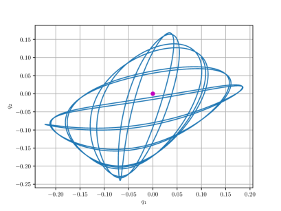
(a)

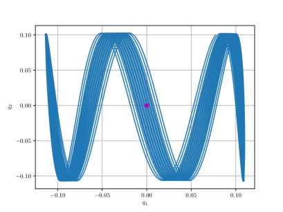
(b)

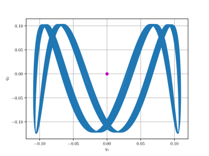
(c)

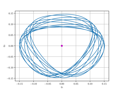
(d)

Figure 1: Trajectories of the generalized Hénon-Heiles Hamiltonian (37) in the various integrable cases and in the chaotic case. We used the odeint integrator from scipy [41] with a regular mesh of $N=2^{25}$ points in the interval $[0,10\times 2\pi/\omega_{1}]$ and $\alpha=2.1$. The magenta dot is the stable equilibrium point $(0,0)$.

Remark 5.

We underline the fact that our method, as a consequence of Corollary 2, is not able to distinguish between integrable and non-integrable cases. The integrable cases of the generalized Hénon-Heiles system (37) were found in [17, 9, 30] by means of the so-called Painlevé test, i.e requiring that the solutions of the equations of motion possess the Painlevé property [63, 64, 65, 29, 28]. It is said that a differential equation possesses the Painlevé property when the only movable singularities are poles (for a modern exposition see [19, 40]). Therefore, one may think that our method is stronger than the Painlevé test which instead can also yield integrability and not maximal superintegrability. However, it is easy to see that statements made using the Painlevé test and our approach are usually not comparable, i.e. when one method fails, the other can succeed and viceversa. To make clear this point, let us discuss the example of the anisotropic caged oscillator.

3.2 The anisotropic caged oscillator

Let us consider the Hamiltonian:

$$H_{\text{c.o.}}=\frac{1}{2}\left(p_{1}^{2}+p_{2}^{2}+p_{3}^{2}\right)+\frac{\omega^{2}}{2}\left(l_{1}^{2}q_{1}^{2}+l_{2}^{2}q_{2}^{2}+l_{3}^{2}q_{3}^{2}\right)+\frac{\alpha_{1}}{2q_{1}^{2}}+\frac{\alpha_{2}}{2q_{2}^{2}}+\frac{\alpha_{3}}{2q_{3}^{2}},$$ (49)

where $l_{k}$ are integers, $\omega$ a positive real number and $\alpha_{k}$ real constants. This system, which was proved to be maximally superintegrable in [25], represents a generalization of the so-called Smorodinski-Winternitz oscillator [27, 24], corresponding to the case $l_{1}=l_{2}=l_{3}=1$. The Lagrangian associated to (49) is given by:

$$L_{\text{c.o.}}=\frac{1}{2}\left(\dot{q}_{1}^{2}+\dot{q}_{2}^{2}+\dot{q}_{3}^{2}\right)-\frac{\omega^{2}}{2}\left(l_{1}^{2}q_{1}^{2}+l_{2}^{2}q_{2}^{2}+l_{3}^{2}q_{3}^{2}\right)-\frac{\alpha_{1}}{2q_{1}^{2}}-\frac{\alpha_{2}}{2q_{2}^{2}}-\frac{\alpha_{3}}{2q_{3}^{2}},$$ (50)

and the Euler-Lagrange equations corresponding to (50) are:

$$\ddot{q}_{k}+l_{k}^{2}\omega^{2}q_{k}=\frac{\alpha_{k}}{q_{k}^{3}},\quad k=1,2,3.$$ (51)

If $\alpha_{k}$ is positive for $k=1,2,3$ we have the following equilibrium positions:

$$q_{k}^{(\pm)}=\pm\left(\frac{\alpha_{k}}{l_{k}^{2}\omega^{2}}\right)^{1/4},\quad k=1,2,3.$$ (52)

From equation (19) we introduce:

$$q_{k}=q_{k}^{(\pm)}+\varepsilon Q_{k},\quad k=1,2,3.$$ (53)

Then, the linearized system is given by:

$$\ddot{Q}_{k}+4l_{k}^{2}\omega^{2}{Q_{k}}=0,\quad k=1,2,3.$$ (54)

The system is already in normal form and the fundamental frequencies are $\boldsymbol{\omega}=\left(2l_{1}\omega,2l_{2}\omega,2l_{3}\omega\right)$. The ratios of the fundamental frequencies are rational as long as $l_{k}$ are integers. To check if this property is preserved at higher order we perform the multiple-scale expansion of the $Q_{k}$, where $k=1,2,3\,$, using three trivial time scales $t_{i}$ (9) with $i=0,1,2$:

$$Q_{k}=Q_{k}^{(0)}\left(t_{0},t_{1},t_{2}\right)+\varepsilon Q_{k}^{(1)}\left(t_{0},t_{1},t_{2}\right)+\varepsilon^{2}Q_{k}^{(2)}\left(t_{0},t_{1},t_{2}\right)+\mathcal{O}\left(\varepsilon^{3}\right),\quad k=1,2,3.$$ (55)

We substitute (55) into (53) and then into (51). Solving the obtained equations we get the following solution:

$$Q_{k}=R_{k}\cos\left(2l_{k}\omega+\varphi_{k}\right),\quad k=1,2,3,$$ (56)

where $R_{k}$ and $\varphi_{k}$ are integration constants. We have then that the first order condition is unaltered, and our approach gives affirmative output, suggesting maximal superintegrability. On the other hand the system (51) does not pass the Painlevé test. In fact, let us assume to have a movable singular point $t_{0}$ with the following behavior in a neighborhood of $t_{0}$:

$$q_{k}=c^{(k)}_{0}(t-t_{0})^{\mu_{k}}+\mathcal{O}\left(\left|t-t_{0}\right|^{\mu_{k}+1}\right),\quad k=1,2,3.$$ (57)

Inserting this ansatz into the equations of motion (51), the possible balances which yields the value of the $\mu_{k}$, are $\mu_{k}=0,1/2$ for $k=1,2,3$. This means that the solutions of (51) is either expressible in Taylor series, then no singularities occur, or it possesses a branch cut, i.e. the behavior is algebraic. In both cases it does not possess movable poles. Moreover, it is easy to show that the series expansion of the solutions of (51) when $\mu_{k}=1/2$ is of the form:

$$q_{k}=\sum_{n=0}^{\infty}c_{n}^{(k)}\left(t-t_{0}\right)^{n+1/2},$$ (58)

i.e. is a Puiseux series [68, 69, 75]. Therefore, using the Painlevé analysis it is not possible to infer the maximal superintegrability of the caged anisotropic oscillator (49), whereas with our method it is. We underline that it is known that there exists many integrable systems which do not possess the Painlevé property, but only the so-called weak Painlevé property, which allows the appearance of branch cuts as in (58). Examples of this kind of systems can be found in [71, 21, 1, 2].

A complete discussion and some graphs of the trajectories of the anisotropic caged oscillator (49) can be found in [25].

Moreover, we observe that the generalization of this example to the $n$ dimensional case, i.e. to:

$$H_{\text{c.o.}}^{(n)}=\sum_{k=1}^{n}\left(\frac{p_{k}^{2}}{2}+\frac{\omega^{2}}{2}l_{k}^{2}q_{k}^{2}+\frac{\alpha_{k}}{2q_{k}^{2}}\right),$$ (59)

where $l_{k}$ are integers and $\alpha_{k}$ and $\omega$ real numbers, is trivial. Using our method we obtain that this system can be superintegrable whereas using the Painlevé analysis we obtain that the behavior near a movable starting point $t_{0}$ is algebraic. In both cases the required expansion is in the form (56) and (58) respectively, with $k$ varying in $\Set{1,2,\dots,n}$. Indeed, in [74] it was showed that the $n$-dimensional caged anisotropic oscillator (59) is maximally superintegrable.

In the next Subsection we will discuss another known example where our method suggest maximal superintegrability.

3.3 The TTW system

In this Subsection we apply the method outlined above to the Tremblay-Turbiner-Winternitz (TTW) system [78], namely:

$$H_{\text{TTW}}=\frac{1}{2}\biggl{(}p_{r}^{2}+\frac{p_{\varphi}^{2}}{r^{2}}\biggl{)}+\frac{1}{2}\omega^{2}r^{2}+\frac{k^{2}}{2r^{2}}\left(\frac{\alpha}{\cos^{2}(k\varphi)}+\frac{\beta}{\sin^{2}(k\varphi)}\right),$$ (60)

where $r$ and $\varphi$ are polar coordinates and $p_{r}$ and $p_{\varphi}$ the associated generalized momenta. The TTW system (60) was introduced in [78] where it was shown to be integrable. Moreover the authors analyzing the structure of the solutions suggested that the system should have been superintegrable (and hence maximally superintegrable since we are in the plane) for every rational $k$.

The proof of superintegrability was accomplished successively, first for odd $k$ [70] and then in the general case for rational $k$ [42, 43]. In this paper we will not use the original formulation of the TTW system. Instead, we will use the following one presented in [73]:

$$\mathcal{H}_{\text{TTW}}=k^{2}(q_{1}^{2}+q_{2}^{2})^{\frac{k-1}{k}}\left[\frac{1}{2}\left(p_{1}^{2}+p_{2}^{2}\right)+\frac{\omega^{2}}{2k^{2}}\left(q_{1}^{2}+q_{2}^{2}\right)^{\frac{2}{k}-1}+\frac{\alpha}{2q_{1}^{2}}+\frac{\beta}{2q_{2}^{2}}\right].$$ (61)

The Hamiltonian (61) is obtained from the Hamiltonian (60) from two successive canonical transformations. The first one is the following:

$$r\cos\varphi=\frac{z+\bar{z}}{2}, \quad\cos\varphi\,p_{r}-\frac{\sin\varphi}{r}\,p_{\varphi}=p_{z}+p_{\bar{z}},$$ (62a)

$$r\sin\varphi=\frac{z-\bar{z}}{2\mathrm{i}}, \quad\sin\varphi\,p_{r}+\frac{\cos\varphi}{r}\,p_{\varphi}=\text{i}(p_{z}-p_{\bar{z}}),$$ (62b)

where $z$ and $\bar{z}$ are complex conjugate variables. The application of the transformation (62) to the Hamiltonian (60) yields the new Hamiltonian:

$$H_{\text{TTW}}^{\mathbb{C}}=2p_{z}p_{\bar{z}}+\frac{\omega^{2}}{2}z\bar{z}+\frac{2\alpha k^{2}z^{k-1}\bar{z}^{k-1}}{\left(z^{k}+\bar{z}^{k}\right)^{2}}-\frac{2\beta k^{2}z^{k-1}\bar{z}^{k-1}}{\left(z^{k}-\bar{z}^{k}\right)^{2}}.$$ (63)

At this point, using the canonical transformation:

$$q_{1}=\frac{1}{2}\left(z^{k}+\bar{z}^{k}\right), \quad p_{1}=\frac{1}{k}\left(z^{1-k}p_{z}+\bar{z}^{1-k}p_{\bar{z}}\right),$$ (64a)

$$q_{2}=\frac{1}{2\mathrm{i}}\left(z^{k}-\bar{z}^{k}\right), \quad p_{2}=\frac{\mathrm{i}}{k}\left(z^{1-k}p_{z}-\bar{z}^{1-k}p_{\bar{z}}\right),$$ (64b)

in the Hamiltonian (63) we obtain the Hamiltonian (61). The form (61) is preferable for our analysis, since the coordinates $\left(q_{1},q_{2}\right)$ are unbounded and take values in $\mathbb{R}^{2}$.

As noted in [73] the form (61), apart from the “conformal” factor $\left(q_{1}^{2}+q_{2}^{2}\right)^{\frac{k-1}{k}}$, is a caged isotropic nonlinear oscillator [24, 25]. Now, we will show an argument which can suggest the superintegrability for rational $k$ of the TTW system in the form (61). The Lagrangian corresponding to (61) is given by:

$$\mathcal{L}_{\text{TTW}}=\frac{1}{2k^{2}}\left(q_{1}^{2}+q_{2}^{2}\right)^{-{\frac{k-1}{k}}}\left(\dot{q}_{1}^{2}+\dot{q}_{2}^{2}\right)-\frac{\omega^{2}}{2}\left(q_{1}^{2}+q_{2}^{2}\right)^{\frac{1}{k}}-\frac{{k}^{2}}{2}\left(q_{1}^{2}+q_{2}^{2}\right)^{{\frac{k-1}{k}}}\left(\frac{\alpha}{q_{1}^{2}}+\frac{\beta}{q_{2}^{2}}\right).$$ (65)

Its Euler-Lagrange equations are:

$$\begin{aligned} \phantom{+k}\left(q_{1}^{2}+q_{2}^{2}\right)^{{\frac{1}{k}}-1}\left(\frac{1}{k^{2}}\ddot{q}_{1}+\frac{{\omega}^{2}}{k}q_{1}\right)&-\frac{1}{k^{3}}\left(k-1\right)\left(q_{1}^{2}+q_{2}^{2}\right)^{-{\frac{2k-1}{k}}}\left[q_{1}\left(\dot{q}_{1}^{2}-\dot{q}_{2}^{2}\right)+2q_{2}\dot{q}_{1}\dot{q}_{2}\right]\\ &-k\left(q_{1}^{2}+q_{2}^{2}\right)^{-{\frac{1}{k}}}\left[\frac{\alpha}{q_{1}^{3}}\left(q_{1}^{2}+kq_{2}^{2}\right)-\frac{\beta}{q_{2}^{2}}\left(k-1\right)q_{1}\right]=0,\end{aligned}$$ (66a)

$$\begin{aligned} \phantom{+k}\left(q_{1}^{2}+q_{2}^{2}\right)^{{\frac{1}{k}-1}}\left(\frac{1}{k^{2}}\ddot{q}_{2}+\frac{{\omega}^{2}}{k}q_{2}\right)&-\frac{1}{k^{3}}\left(k-1\right)\left(q_{1}^{2}+q_{2}^{2}\right)^{-{\frac{2k-1}{k}}}\left[q_{2}\left(\dot{q}_{2}^{2}-\dot{q}_{1}^{2}\right)+2q_{1}\dot{q}_{1}\dot{q}_{2}\right]\\ &+k\left(q_{1}^{2}+q_{2}^{2}\right)^{-{\frac{1}{k}}}\left[\frac{\alpha}{q_{1}^{2}}\left(k-1\right)q_{2}-\frac{\beta}{q_{2}^{3}}\left(kq_{1}^{2}+q_{2}^{2}\right)\right]=0.\end{aligned}$$ (66b)

Restricting to the case $\alpha,\beta>0$ we can define $\alpha\doteq A^{4}$ and $\beta\doteq B^{4}$ with $A,B>0$. In this case the real equilibrium positions of the TTW system (65) are given by:

$$q_{1}^{(\pm)}=\pm A\left(\frac{k}{\omega}\right)^{\frac{k}{2}}\left(A^{2}+B^{2}\right)^{\frac{k-1}{2}},\quad q_{2}^{(\pm)}=\pm B\left(\frac{k}{\omega}\right)^{\frac{k}{2}}\left(A^{2}+B^{2}\right)^{\frac{k-1}{2}}.$$ (67)

Due to the fact that the system (65) is symmetric under the discrete transformations $q_{1}\to-q_{1}$ and $q_{2}\to-q_{2}$ we can consider only the equilibrium positions labeled by $(+,+)$ in (67). From equation (19) we introduce:

$$q_{1}=q_{1}^{(+)}+\varepsilon Q_{1},\quad q_{2}=q_{2}^{(+)}+\varepsilon Q_{2}.$$ (68)

Inserting equation (68) into the Euler-Lagrange equations (66) and expanding in Taylor series with respect to $\varepsilon$, we obtain as coefficients of $\varepsilon$ the following linearized equations:

$$\ddot{Q}_{1}+{\frac{4{\omega}^{2}\left({A}^{2}+{k}^{2}{B}^{2}\right)}{{A}^{2}+{B}^{2}}}Q_{1}+{\frac{4{\omega}^{2}AB\left(1-{k}^{2}\right)}{{A}^{2}+{B}^{2}}}Q_{2}=0\,,$$ (69a)

$$\ddot{Q}_{2}+{\frac{4{\omega}^{2}AB\left(1-{k}^{2}\right)}{{A}^{2}+{B}^{2}}}Q_{1}+{\frac{4{\omega}^{2}\left({k}^{2}{A}^{2}+{B}^{2}\right)}{{A}^{2}+{B}^{2}}}Q_{2}=0\,.$$ (69b)

We introduce the normal coordinates $N_{1}$ and $N_{2}$ through the linear transformation:

$$\begin{bmatrix}Q_{1}\\ Q_{2}\end{bmatrix}=\begin{bmatrix}A&B\\ B&-A\\ \end{bmatrix}\begin{bmatrix}N_{1}\\ N_{2}\end{bmatrix}$$ (70)

obtaining from (69) the following linearized system:

$$\ddot{N}_{1}+4\omega^{2}N_{1}=0,\quad\ddot{N}_{2}+4k^{2}\omega^{2}N_{2}=0.$$ (71)

In this case the fundamental frequencies are $\boldsymbol{\omega}=\left(2\omega,2k\omega\right)$, which means that we can expect (maximal) superintegrability only if $k$ is rational, just as suggested in [78]. Now, we use a multiple-scale expansion to show that at higher orders the periodicity is preserved. Thus, this time we perform a multiple-scale expansion in terms of the normal coordinates $N_{1}$ and $N_{2}$, with the three trivial time scales $t_{i}$ (9) with $i=0,1,2$:

$$N_{k}=N_{k}^{(0)}\left(t_{0},t_{1},t_{2}\right)+\varepsilon N_{k}^{(1)}\left(t_{0},t_{1},t_{2}\right)+\varepsilon^{2}N_{k}^{(2)}\left(t_{0},t_{1},t_{2}\right)+O\left(\varepsilon^{3}\right),\quad k=1,2.$$ (72)

Then, we can insert this expansion in (68-70) and into (66). Expanding in Taylor series with respect to $\varepsilon$ and taking coefficients up to the second order yields a sequence of systems which can readily be solved. Surprisingly enough, if we do not know the properties of the TTW system (61), we find that there are no corrective terms to the fundamental frequencies and the asymptotic solution, valid up to $\varepsilon^{2}t=\mathcal{O}\left(1\right)$, is just given by:

$$N_{1} =R_{1}\cos\left(2\omega t+\varphi_{1}\right)+\mathcal{O}\left(\varepsilon\right),$$ (73a)

$$N_{2} =R_{2}\cos\left(2k\omega t+\varphi_{2}\right)+\mathcal{O}\left(\varepsilon\right),$$ (73b)

where $R_{k}$ and $\varphi_{k}$ with $k=1,2$ are integration constants. This just shows that the ratio is preserved and that the TTW system (61) can be superintegrable. Moreover, this also shows that the multiple-scale expansion collapses into a standard perturbative expansion of the form:

$$N_{k}(t)=\sum_{i=0}^{\infty}\varepsilon^{i}N_{k}^{(i)}(t),\quad k=1,2.$$ (74)

The fact that there are no corrections to the fundamental frequencies reflects the property of isochronicity of the TTW system, since the frequency of oscillation of the system is independent from the initial values [79, 14]. Without giving a complete account of the form of the orbits of the TTW system [79, 73], we show some numerical examples in Figure 2.

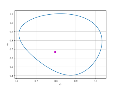
(a)

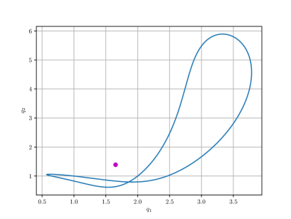
(b)

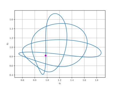
(c)

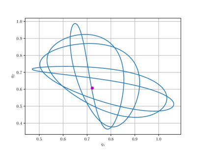
(d)

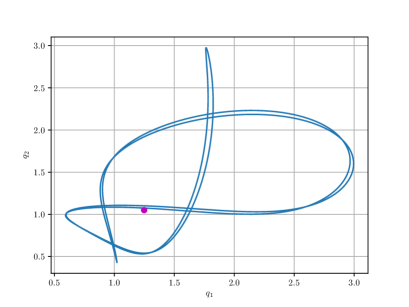
(e)

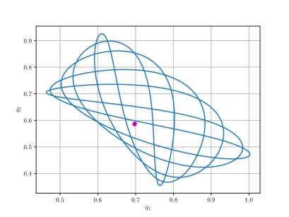
(f)

Figure 2: Trajectories of the TTW Hamiltonian (61) for different values of $k=k_{\text{n}}/k_{\text{d}}$ with integer $k_{\text{n}}$ and $k_{\text{d}}$ with fixed parameters $\omega=1/2$, $\alpha=1/10$ and $\beta=1/20$. We used the odeint integrator from scipy [41] with a regular mesh of $N=2^{25}$ points in the interval $[0,2\pi k_{\text{n}}k_{\text{d}}/\omega]$. The magenta dots are the stable equilibrium points labeled by $\left(+,+\right)$ in (67).

3.4 The Drach system

In this Subsection we present a new result about what we are going to call the Drach system. In 1935 Drach [22] carried out the first systematic search for integrable systems with a third-order integral of motion in two dimensions. He conducted his search in a two-dimensional complex space $\mathbb{E}_{2}\left(\mathbb{C}\right)$ and found ten potentials. These potentials have been subject of further investigations in more recent times [80, 81, 77]. In particular one of these potentials can be rewritten in real form as:

$$H_{\text{Drach}}=\frac{1}{2}\left(p_{1}^{2}+p_{2}^{2}\right)+\frac{aq_{2}+b+c(4q_{1}^{2}+3q_{2}^{2})}{q_{1}^{2/3}},$$ (75)

where a priori $a$, $b$ and $c$ are real parameters. In [67] a particular case of (75) with $c=0$ was considered and showed to be (maximally) superintegrable with a third-order and a fourth-order additional integral of motion.

We will refer to this particular case as the Drach-Post-Winternitz (DPW) system. The DPW system is important since its quantum version was the first nonseparable (maximally) superintegrable system ever found. In [59], using the so-called reduction method [56, 57, 58], it was shown to be reducible to the third-order trivial equation $X^{\prime\prime\prime}=0$.

At the end of their paper the authors in [67] state that:

“For $c\neq 0$ (31) [here (75)] does not allow a fourth-order integral, though it still might be superintegrable.”

leaving open the question whether or not the “full” Drach system (75) is (maximally) superintegrable. Now, we show using the argument proposed in Section 2 that the Drach system is in general not (maximally) superintegrable. Indeed, the Lagrangian corresponding to (75) is:

$$L_{\text{Drach}}=\frac{1}{2}\left(\dot{q}_{1}^{2}+\dot{q}_{2}^{2}\right)-\frac{aq_{2}+b+c(4q_{1}^{2}+3q_{2}^{2})}{q_{1}^{2/3}}.$$ (76)

The corresponding Euler-Lagrange equations are:

$$\ddot{q}_{1}+8cq_{1}^{1/3}-\frac{2}{3}\frac{aq_{2}+b+c(4q_{1}^{2}+3q_{2}^{2})}{q_{1}^{5/3}} =0,$$ (77a)

$$\ddot{q}_{2}+\frac{a+6cq_{2}}{q_{1}^{2/3}} =0.$$ (77b)

We have two equilibrium positions:

$$q_{1}^{(\pm)}=\pm\frac{\eta}{24c},\quad q_{2}^{(0)}=-\frac{a}{6c},$$ (78)

where we have introduced the shorthand notation:

$$72bc-6a^{2}=\eta^{2}.$$ (79)

The presence of $b$ here is necessary in order to have real solutions to the equations of the equilibrium conditions. Therefore, from now on we will assume $b>a^{2}/(12c)$ and $c\neq 0$, otherwise (78) loses its meaning. We observe that the $c=0$ is just the DPW case [67], which has no equilibrium solutions. From equation (19) we obtain:

$$q_{1}=q_{1}^{(\pm)}+\varepsilon Q_{1},\quad q_{2}=q_{2}^{(0)}+\varepsilon Q_{2}$$ (80)

with $q_{1}^{(\pm)}$ and $q_{2}^{(0)}$ given by (78). The equilibrium position with $q_{1}^{(-)}$ is not stable for every value of the parameters, whereas the one with $q^{(+)}$, for $c>0$, yields to the following linearized equations:

$$\ddot{Q}_{1}+\frac{128}{3}\left(\frac{3}{\eta}\right)^{2/3}c^{5/3}Q_{1} =0,$$ (81a)

$$\ddot{Q}_{2}+24\left(\frac{3}{\eta}\right)^{2/3}c^{5/3}Q_{2} =0.$$ (81b)

The system is already in normal form and the fundamental frequencies are given by:

$$\omega_{1}^{(0)}=\frac{8\sqrt{6}c^{5/6}3^{1/3}}{3\eta^{1/3}},\quad\omega_{2}^{(0)}=\frac{2\sqrt{6}c^{5/6}3^{1/3}}{\eta^{1/3}}.$$ (82)

The ratio of the two fundamental frequencies is rational:

$$\Delta^{(0)}=\frac{\omega_{1}^{(0)}}{\omega_{2}^{(0)}}=\frac{4}{3}.$$ (83)

At this stage we have that the Drach system (75) might be (maximally) superintegrable. To check what happens at higher order we use a multiple-scale expansion with three trivial time scales (9) of the form (42). We substitute (42) into (80) and then into the Euler-Lagrange equations (77). Expanding in Taylor series with respect to $\varepsilon$, and then carrying out the computations, we get the following solution:

$$Q_{1}=R_{1}\cos\left[\left(\omega_{1}^{(0)}+\omega_{1}^{(2)}\varepsilon^{2}\right)t+\varphi_{1}\right]+\mathcal{O}\left(\varepsilon\right),$$ (84a)

$$Q_{2}=R_{2}\cos\left[\left(\omega_{2}^{(0)}+\omega_{2}^{(2)}\varepsilon^{2}\right)t+\varphi_{2}\right]+\mathcal{O}\left(\varepsilon\right).$$ (84b)

Here $R_{i}$ and $\varphi_{i}$ are constants of integration, $\omega_{i}^{(0)}$ are given by (82) and the corrections to the frequencies are given by:

$$\omega_{1}^{(2)} =-\frac{8}{45}\frac{\sqrt{6}c^{17/6}3^{1/3}\left(400R_{1}^{2}+513R_{2}^{2}\right)}{\eta^{7/3}},$$ (85a)

$$\omega_{2}^{(2)} =-\frac{2}{5}\frac{\sqrt{6}c^{17/6}3^{1/3}\left(304R_{1}^{2}+54R_{2}^{2}\right)}{\eta^{7/3}}.$$ (85b)

The ratio of these additional frequencies is no longer given by (83) and in fact we can see that:

$$\Delta^{(2)}=\frac{\omega_{1}^{(0)}+\omega_{1}^{(2)}\varepsilon^{2}}{\omega_{2}^{(0)}+\omega_{2}^{(2)}\varepsilon^{2}}=\frac{4}{3}+\frac{4}{45}\frac{c^{2}}{\eta^{2}}\left(512R_{1}^{2}-351R_{2}^{2}\right)\varepsilon^{2}+\mathcal{O}\left(\varepsilon^{4}\right).$$ (86)

As discussed in Section 2 this behavior is not consistent with a (maximally) superintegrable system. Therefore, we are led to conclude that in general the Drach system is an integrable, but not a superintegrable system. This does not exclude the possibility of the existence of other (maximally) superintegrable subcases, especially in the range of parameters which cannot be covered with our technique. For example, it is worth mentioning that the DPW system, which arises as singular limit as $c\to 0$, does not possess closed orbits. This leaves open the question whether or not there exists other superintegrable subcases without closed orbits. To give the feeling of the form of the trajectories of the Drach system, and of the fact that they are non-periodic we show some numerical examples in Figure 3.

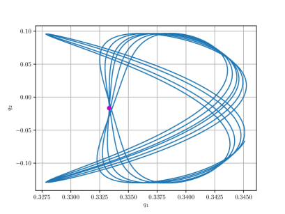
(a)

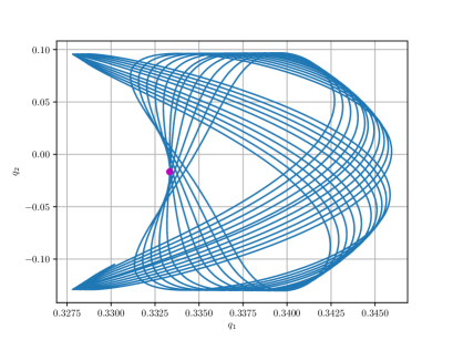
(b)

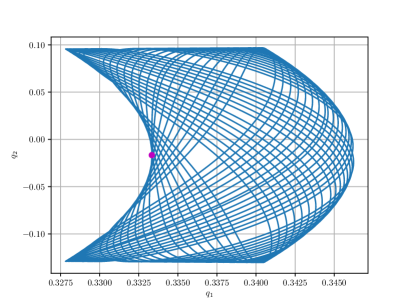
(c)

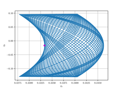
(d)

Figure 3: Trajectories for the maps (77) with parameters $a=0.1$, $\eta=8$, $c=1$. We used the odeint integrator from scipy [41] with a regular mesh of $N=2^{25}$ points. The magenta dot is the stable equilibrium point labeled by $(+)$ in (78).

To conclude this paper we wish to show with an explicit example how this approach can be used to suggest maximal superintegrability of a class of Hamiltonian systems. We will give a proof of Bertrand’s theorem [7] using our method. This will also point out the main differences between our approach and the one followed in [86].

3.5 Central force potentials: Bertrand’s theorem

In this Subsection we give an alternative proof of the following:

Theorem 4 (Bertrand [7]).

Assume we are given the Hamiltonian in the Euclidean plane:

$$H_{k,\alpha}=\frac{1}{2}\left(p_{r}^{2}+\frac{p_{\varphi}^{2}}{r^{2}}\right)+kr^{\alpha}$$ (87)

where $r\in\mathbb{R}^{+}$ and $\varphi\in[0,2\pi)$ are polar coordinates, $p_{r}$ and $p_{\varphi}$ the respective momenta, and $k$ and $\alpha$ are real constants. Then, the only two cases for which all bounded orbits are closed are those corresponding to $\alpha=2$, $k>0$ and $\alpha=-1$, $k<0$, i.e. the isotropic harmonic oscillator and the Kepler system.

Proof.

We will give a direct proof of this theorem, i.e. without resorting to the equation of the orbits [82, 47, 3], by using the multiple scales approach. The Lagrangian associated with (87) is:

$$L_{k,\alpha}=\frac{1}{2}\left(\dot{r}^{2}+r^{2}\dot{\varphi}^{2}\right)-kr^{\alpha}.$$ (88)

The Euler-Lagrange equations corresponding to (88) are given by:

$$r^{2}\ddot{\varphi}+2r\dot{\varphi}\dot{r} =0,$$ (89a)

$$\ddot{r}-r\dot{\varphi}^{2}+k\alpha r^{\alpha-1} =0.$$ (89b)

It is easy to check that in this case there are no equilibrium positions, so the method does not seem applicable. We recall that, in order to apply the procedure of Section 2, we need a stable equilibrium solution to check whether the perturbative expansion around the stable point gives rise to closed orbits or not. Due to the radial symmetry of the Hamiltonian (87) it is natural to make a different ansatz: we search for the existence of circular orbits, i.e. a two-parameter family of solutions of the form:

$$r=r_{0},\quad\varphi=\omega_{0}t+\varphi_{0},$$ (90)

where $\omega_{0}=\omega_{0}\left(r_{0}\right)$. The motion defined by (90) is called circular since it represents the equation of a circle in polar coordinates [47]. Inserting the ansatz into the equations of motion (89) we obtain:

$$\omega_{0}=\sqrt{k\alpha}r_{0}^{\alpha/2-1},$$ (91)

which implies that there exist circular orbits for the system (89) if $k\alpha>0$, i.e. $k>0$ and $\alpha>0$ or $k<0$ and $\alpha<0$. We underline that circular orbits are exact solutions and their property is to maximize the angular momentum:

$$\ell=r^{2}\dot{\varphi},$$ (92)

being both $r$ and $\dot{\varphi}$ constants. Since every other kind of orbit will have smaller angular momentum, when circular orbits do not exist, i.e. when $k\alpha<0$, there are no bounded trajectories. We note that due to the radial symmetry we can always suppose $\varphi_{0}\equiv 0$ in (90).

Therefore, we can restrict the analysis to the range of parameters $k\alpha>0$. We turn to investigate the stability of circular orbits in this range. We introduce the expansion of nearly-circular orbits:

$$r=r_{0}+\varepsilon\rho,\quad\varphi=\omega_{0}\left(t+\varepsilon\theta\right),$$ (93)

where $\rho=\rho\left(t\right)$, $\theta=\theta\left(t\right)$ and $\varepsilon\to 0^{+}$. Inserting the expansion (93) into (89), at the first order in $\varepsilon$ we obtain:

$$r_{0}\ddot{\theta}+2\dot{\rho} =0,$$ (94a)

$$\ddot{\rho}-2r_{0}^{\alpha-1}k\alpha\dot{\theta}+\alpha k\left(\alpha-2\right)r_{0}^{\alpha-2}\rho =0.$$ (94b)

The system (94) has the following solution:

$$\rho =\rho_{0}\cos(r_{0}^{\alpha/2-1}\sqrt{k\alpha\left(\alpha+2\right)}t+\beta_{0})+\frac{2r_{0}\Omega_{0}}{\alpha+2},$$ (95a)

$$\theta =\frac{\alpha-2}{\alpha+2}\Omega_{0}t-\frac{2\rho_{0}}{r_{0}^{\alpha/2}\sqrt{k\alpha\left(\alpha+2\right)}}\sin(r_{0}^{\alpha/2-1}\sqrt{k\alpha\left(\alpha+2\right)}t+\beta_{0})+\theta_{0},$$ (95b)

where $\rho_{0}$, $\beta_{0}$, $\Omega_{0}$ and $\theta_{0}$ are constants of integration. The solution (95) implies that the circular orbits are stable if $k\alpha\left(\alpha+2\right)>0$ hence, being $k\alpha>0$, when $\alpha>-2$. When $\alpha<-2$ circular orbits are unstable and we have unbounded motion. Moreover, recalling formula (93), we obtain that at the zero-th order the frequencies are given by $\omega_{0}$ from (91) and by:

$$\bar{\omega}_{0}=r_{0}^{\alpha/2-1}\sqrt{k\alpha\left(\alpha+2\right)}.$$ (96)

Now, due to the fact that $\varphi$ is an angle variable, we have that at the zero-th order the condition for the orbit to be closed is given by $\omega_{0}/\bar{\omega}_{0}\in\mathbb{Q}$. This implies:

$$\Delta^{(0)}=\frac{1}{\sqrt{\alpha+2}}=\frac{n}{m},$$ (97)

where $n$, $m$ are co-prime integers.

To check if this condition is preserved at higher order we perform a multiple-scale expansion with three trivial time scales given by equation (9):

$$\rho =\rho_{0}\left(t_{0},t_{1},t_{2}\right)+\varepsilon\rho_{1}\left(t_{0},t_{1},t_{2}\right)+\varepsilon^{2}\rho_{2}\left(t_{0},t_{1},t_{2}\right)+\mathcal{O}\left(\varepsilon^{3}\right),$$ (98a)

$$\theta =\theta_{0}\left(t_{0},t_{1},t_{2}\right)+\varepsilon\theta_{1}\left(t_{0},t_{1},t_{2}\right)+\varepsilon^{2}\theta_{2}\left(t_{0},t_{1},t_{2}\right)+\mathcal{O}\left(\varepsilon^{3}\right).$$ (98b)

Inserting the expansion (98) into the form of the nearly-circular orbits (93), and then into (89), we obtain the following nearly-circular orbit:

$$r =r_{0}+\varepsilon\frac{2r_{0}\Omega_{0}}{\alpha+2}+\varepsilon\rho_{0}\cos\left[\bar{\omega}_{0}\left(1+\varepsilon\frac{\alpha-2}{\alpha+2}\Omega_{0}+\varepsilon^{2}\bar{\mu}^{(2)}\right)t+\beta_{0}\right]+\mathcal{O}\left(\varepsilon^{2}\right),$$ (99a)

$$\varphi \begin{aligned} &=\omega_{0}\left\{1+\varepsilon\frac{\alpha-2}{\alpha+2}\Omega_{0}+\frac{\varepsilon^{2}}{2}\left(\alpha-2\right)\left[\frac{1}{4}\left(\frac{\rho_{0}}{r_{0}}\right)^{2}(\alpha-1)+\frac{\alpha-4}{\left(\alpha+2\right)^{2}}\Omega_{0}^{2}\right]\right\}t\\ &-\frac{2\varepsilon\omega_{0}\rho_{0}}{r_{0}^{\alpha/2}\sqrt{k\alpha\left(2+\alpha\right)}}\sin\left[\bar{\omega}_{0}\left(1+\varepsilon\frac{\alpha-2}{\alpha+2}\Omega_{0}+\varepsilon^{2}\bar{\mu}^{(2)}\right)t+\beta_{0}\right]+\varepsilon\omega_{0}\theta_{0}+\mathcal{O}\left(\varepsilon^{2}\right),\end{aligned}$$ (99b)

where $\rho_{0}$, $\beta_{0}$, $\Omega_{0}$ and $\theta_{0}$ are constants of integration, $\omega_{0}$ is given by (91), $\bar{\omega}_{0}$ is given by (96) and:

$$\bar{\mu}^{(2)}=\frac{1}{2}(\alpha-2)\left[\frac{1}{6}\left(\frac{\rho_{0}}{r_{0}}\right)^{2}(\alpha-2)+\frac{\alpha-4}{(\alpha+2)^{2}}\Omega_{0}^{2}\right].$$ (100)

Defining:

$$\mu^{(2)}\doteq\frac{1}{2}\left(\alpha-2\right)\left[\frac{1}{4}\left(\frac{\rho_{0}}{r_{0}}\right)^{2}(\alpha-1)+\frac{\alpha-4}{\left(\alpha+2\right)^{2}}\Omega_{0}^{2}\right],$$ (101)

we obtain from (99b) that, at the second order, the frequencies are given by

$$\omega_{2} =\omega_{0}\left(1+\varepsilon\frac{\alpha-2}{\alpha+2}\Omega_{0}+\varepsilon^{2}\mu^{(2)}\right),$$ (102a)

$$\bar{\omega}_{2} =\bar{\omega}_{0}\left(1+\varepsilon\frac{\alpha-2}{\alpha+2}\Omega_{0}+\varepsilon^{2}\bar{\mu}^{(2)}\right).$$ (102b)

We observe that the precision of $\varphi$ in (99b) is of order $\varepsilon^{2}$, but $\omega_{2}$ (102a) is allowed to contain terms of higher order. This is possible since these higher order terms arise when fixing terms of order $\varepsilon$ in the multiple-scale expansion, according to the prescriptions in Section 2. In this sense these are not bona fide higher order terms, but just higher order corrections to the $\mathcal{O}\left(1\right)$ term $\omega_{0}$. Now, due to the fact that $\varphi$ is an angle variable, we have that at the second order the condition for the orbit to be closed is that $\omega_{2}/\bar{\omega}_{2}$ must stay rational. Expanding in Taylor series we can write:

$$\Delta^{(2)}=\frac{\omega_{2}}{\bar{\omega}_{2}}=\frac{1}{\sqrt{\alpha+2}}+\frac{\varepsilon^{2}}{24}\left(\frac{\rho_{0}}{r_{0}}\right)^{2}\frac{(\alpha+1)(\alpha-2)}{\sqrt{\alpha+2}}+\mathcal{O}\left(\varepsilon^{3}\right).$$ (103)

This implies that in addition to the condition (97) we must have either $\alpha=-1$ or $\alpha=2$. Otherwise in the ratio $\omega_{2}/\bar{\omega}_{2}$ there will be terms depending on the initial conditions, which can clearly be purely irrational. We note that if $\alpha=2$, then $k=\kappa^{2}$ and we have $\omega_{2}/\bar{\omega}_{2}=1/2$ whereas if $\alpha=-1$, then $k=-\kappa^{2}$ and we have $\omega_{2}/\bar{\omega}_{2}=1$. This means that in these two cases the proportionality is exact up to the second order. This concludes the proof of the Theorem, since it is known [47, 82, 53] that in the two mentioned cases the bounded orbits are closed. For instance if $\alpha=2$ and $k=\kappa^{2}$ the orbits are given by the following expression:

$$r^{2}(\varphi)=\dfrac{\ell^{2}/E}{1+\sqrt{1-2(\kappa\ell/E)^{2}}\cos\left[2(\varphi-\varphi_{0})\right]},$$ (104)

where $E$ is the total mechanical energy of the system. Equation (104) means that the radius vector describes ellipses centered at the origin. On the other hand, if $\alpha=-1$ and $k=-\kappa^{2}$, the orbits are given by the following expression:

$$r(\varphi)=\dfrac{\ell^{2}/\kappa^{2}}{1+\sqrt{1+2E\ell^{2}/\kappa^{4}}\cos(\varphi-\varphi_{0})}\,.$$ (105)

Equation (105) means that, for bounded motion, the radius vector describes ellipses where the origin is one of the foci. In both cases, the time dependence is recovered by integrating the angular momentum first integral (92):

$$t-t_{0}=\frac{1}{\ell}\int_{\varphi_{0}}^{\varphi}r^{2}\left(\tilde{\varphi}\right)\mathrm{d}\tilde{\varphi}.$$ (106)

This concludes the proof of the Theorem. ∎

In Figure 4 we show some examples of circular orbits and their deformations in the cases highlighted during the proof of Bertrand’s Theorem 4.

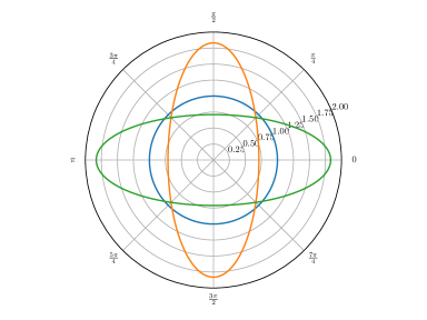
(a) $\alpha=2$: the circular orbit (blue) is stable, and the perturbations are periodic ellipses (orange and green). Exact plot using formula (104).

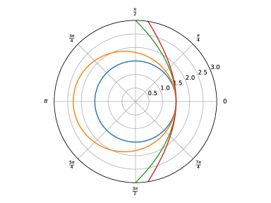
(b)

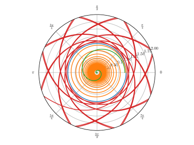
(c)

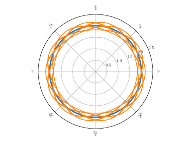
(d)

Figure 4: Circular orbits and their deformations for various values of $\alpha$.

Remark 6.

We remark that the proof of Bertrand’s Theorem 4 can be accomplished using the Poincaré-Lindstedt method [86], which is a particular case of the multiple scales method. We remark, however, that our procedure is more general than the one applied in [86]. In fact, we do not need to resort to the orbit equation and we do not need to use periodicity as a hypothesis, but periodicity arises as a consequence.

Remark 7.

We underline that the proof of Bertrand’s Theorem 4 could have been accomplished in another way using non-inertial reference frames [47, 82, 3]. In fact, let us assume that our motion in the plane is a restriction of a three dimensional motion in $\left(q_{1},q_{2},q_{3}\right)\in\mathbb{R}^{3}$ where along the $q_{3}$-axis there is no dynamics. Then, we can switch to a non-inertial reference frame moving around the $q_{3}$-axis with angular velocity $\boldsymbol{\Theta}=\left(0,0,\Theta\right)$. This corresponds to the following coordinate transformation [47, 82, 3]:

$$r=R,\quad\varphi=\Phi+\Theta t,$$ (107)

where we denoted with capital letters the coordinates in the non-inertial reference system. The transformation (107) brings the Lagrangian (88) into the following form:

$$L_{k,\alpha,\Theta}=\frac{1}{2}\left(\dot{R}^{2}+R^{2}\dot{\Phi}^{2}\right)+\Theta R^{2}\dot{\Phi}+\Theta^{2}R^{2}-kR^{\alpha}.$$ (108)

It is easy to prove that the Euler-Lagrange equations corresponding to (108), differently from those of (88), possess the following equilibrium solutions:

$$R_{0}=\left(\frac{\Theta^{2}}{k\alpha}\right)^{1/\left(\alpha-2\right)},$$ (109)

and $\Phi_{0}$ can be arbitrary in $[0,2\pi)$. Changing the value of $\Theta$ we can change the equilibrium point in the variables $\left(R,\Phi\right)$. E.g. choosing $\Theta=\sqrt{k\alpha}r_{0}^{\alpha/2-1}$, with $r_{0}\in\mathbb{R}^{+}$ every positive real number can be chosen to be the equilibrium point. Therefore, we obtain that the equilibrium positions of the Euler-Lagrange equations corresponding to (108) are given by $\left(r_{0},\Phi_{0}\right)$ with fixed $r_{0}\in\mathbb{R}^{+}$ and for all $\Phi_{0}\in[0,2\pi)$. These equilibrium points then lie on circles centered at $R=0$ of radius $r_{0}$. Adjusting the angular velocity $\Theta$ of the non-inertial reference frame we can change the radius of the circle. This means that these equilibrium points form a two-parameter family of solutions. That is, we have a one-to-one correspondence between the equilibrium positions of the Euler-Lagrange equations corresponding to (108) and the circular orbits (90). At this point one just needs to perform the usual analysis with the derived equilibrium positions and with the Euler-Lagrange equations corresponding to (108). Inverting the point transformation (107) we then obtain the result in the original inertial reference frame. These reasoning underlines what is well-known in Celestial Mechanics [53], i.e. that using conveniently non-inertial reference frames, in some cases it is possible to map particular solutions to equilibrium points. This fact can be also used, in principle, in other cases where no equilibrium solutions exist, but it is possible to find simple classes of solutions.

4 Conclusions and outlook

In this paper we presented a simple method which allows to establish if a Hamiltonian system may be or not maximally superintegrable. The main benefit of this approach is the fact that it is algorithmic and relies on the well-established method of the multiple scales expansion. As stated in Section 2 the multiple scales analysis proved to be very useful in the theory of integrable systems in infinite dimensions. We believe that the procedure presented in this paper can be thought as its finite dimensional analog. Indeed, it has been observed that integrable systems in infinite dimensions are, as a matter of fact, maximally superintegrable. The generalized symmetries of these equations form infinite dimensional non-Abelian algebras (the Orlov-Shulman symmetries) with infinite dimensional Abelian subalgebras of commuting flows [60, 61, 62]. Most notably, the multiple scales method has never been systematically applied to finite dimensional systems.

We applied this method to five relevant examples in order to understand its features and its limits:

1. The generalized Hénon-Heiles system (37).

2. The anisotropic caged oscillator (49).

3. The TTW system (61).

4. The Drach system (75).

5. The central force Hamiltonian (87).

From the example of the generalized Hénon-Heiles system (37) we explicitly showed that our approach, based only on equilibrium positions and perturbative expansions, cannot distinguish between chaoticity and integrability, but only between non maximal superintegrability and maximal superintegrability. From the example of the anisotropic caged oscillator (49) we showed that our test can detect maximal superintegrability where the Painlevé test fails. This shows that our maximal superintegrability test is not necessarily stronger than the Painlevé property as the example of the generalized Hénon-Heiles system could have suggested. This implies that the application of these two different tests, both based on the analysis of the property of the solution of a mechanical system, can be thought as complementary. From the example of the TTW system (61) we showed how the results of our technique are able to suggest the superintegrability of this well-known model. Furthermore, with the Drach system (75) we gave a practical example of the method by showing that this system is, in general, not (maximally) superintegrable. Finally, with the last example we gave some hints on how this approach could be applied to classify maximally superintegrable systems by presenting a direct proof of Bertrand’s Theorem 4 . During the proof we gave a slight generalization of the algorithm presented in Section 2. We remark that this generalization can be applied every time a parametric family of bounded and closed solutions is known. Moreover, we observe that during the proof we have recovered the following Lemma which is interesting on its own:

Lemma 5.

Assume we are given the Hamiltonian in the Euclidean plane $H_{k,\alpha}$ of equation (87). Then, if $k\alpha>0$ and $\alpha>-2$ circular orbits (90) exist and are stable.

Amongst the systems admitting stable circular orbits the isotropic harmonic oscillator and the Kepler system occupy a special place, having their finite orbits closed and periodic. This emphasizes how in the classification problem a perturbative approach like ours phase out the generic cases, leaving only those with interesting properties. The remaining cases can then be treated directly, and their properties are usually manifest. Moreover, we could interpret the fact that the isotropic harmonic oscillator and the Kepler system possess special properties, beneath a huge amount of similar systems, as a finite dimensional analog of the fact that almost every evolution equation possesses a $1$-soliton solution, whereas $N$-soliton solutions are a unique feature of integrable equations. Furthermore, the many non-integrable equations possessing also a $2$-soliton solution can be seen as the analog of the potentials satisfying the hypothesis of Lemma 5. Indeed, the true distinction between the integrable and the non-integrable cases arises when the existence of a $3$-soliton solution is required. This is because the interaction of three solitons of a non-integrable evolution equations becomes destructive. In the same way in our finite dimensional case the closeness of circular orbits is not preserved when we arrive at the third time scale. We mention that the existence of $3$-soliton solutions have been used to classify soliton equations in [33, 34, 35, 36, 37] using the so-called Hirota bilinear method [38]. We also note that soliton solutions of integrable equations are usually stable with respect to some norm in an appropriate function space [85, 50]. Intuitively the stability of the $N$-soliton solution for an integrable equation can be described as follows: given “sufficiently regular” and rapidly decreasing initial data it is possible to construct the inverse scattering. The evolution of the spectral data then implies that the given initial data will evolve producing a certain number of solitons and a radiative background. The area of the radiative background is “small” compared to that of the solitions. Then, as time grows, the radiative background decays whereas the solitons will keep their form unaltered, since in the collisions only the relative shifts will change. This comment underlines another possible analogy between the finite and the infinite dimensional case.

To conclude we have that, in general, maximal superintegrability can be proved with the usual approaches, see [51] and references therein, but the procedure we presented can be used as a sieve test for maximally superintegrable systems. Based on this evidence we think that the application of this approach in a more general setting, where instead of arbitrary constants, namely $\alpha$ and $k$ in Bertrand’s Theorem 4, we have arbitrary functions may be a new way to classify families of maximally superintegrable systems. We reserve the application of this method in this more general setting to future works.

Appendix A Orbits of (87) if $\boldsymbol{\alpha=-2}$ or $\boldsymbol{\alpha=6}$

For a system with radial symmetry the orbits can be computed in general using the so-called orbit equation [82, 47, 3, 53]:

$$\derivative[2]{u}{\varphi}+u=\frac{k\alpha}{\ell^{2}}u^{-\alpha-1},$$ (110)

where $u=1/r$ and $\varphi$ is the new dependent variable defined through the differential substitution obtained from (92):

$$\mathrm{d}t=\frac{r^{2}}{\ell}\mathrm{d}\varphi.$$ (111)

The differential substitution (111) is possible since $\ell$ is constant along the solutions of (89). Performing the differential substitution (111) we have that (89a) is satisfied identically and (89b) is transformed into:

$$\frac{\ell}{r^{2}}\derivative{\varphi}\left(\frac{\ell}{r^{2}}\derivative{r}{\varphi}\right)-\frac{\ell^{2}}{r^{3}}=-k\alpha r^{\alpha-1}.$$ (112)

Applying the transformation $r=1/u$ equation (110) follows. Here, we will concentrate on the two cases $\alpha=-2$ and $\alpha=6$.

Case $\boldsymbol{\alpha=-2}$.

If $\alpha=-2$ then the orbit equation (110) is linear. Due to the Remark made during the proof of Bertrand’s Theorem we impose $k=-\kappa^{2}/2$. Defining:

$$\lambda\doteq 1-\frac{\kappa^{2}}{\ell^{2}}\,,$$ (113)

the solutions in terms of $r$ are [82, 47, 3, 53]:

$$r=\begin{cases}\displaystyle\frac{r_{0}\ell}{\ell\cos\left[\sqrt{\lambda}\left(\varphi-\varphi_{0}\right)\right]-r_{0}\dot{r}_{0}\sin\left[\sqrt{\lambda}\left(\varphi-\varphi_{0}\right)\right]},&\text{if $\lambda>0$},\\ \displaystyle\frac{r_{0}\ell}{\ell\cosh\left[\sqrt{-\lambda}\left(\varphi-\varphi_{0}\right)\right]-r_{0}\dot{r}_{0}\sinh\left[\sqrt{-\lambda}\left(\varphi-\varphi_{0}\right)\right]},&\text{if $\lambda<0$},\\ \displaystyle\frac{r_{0}\ell}{\ell-r_{0}\dot{r}_{0}\left(\varphi-\varphi_{0}\right)}.&\text{if $\lambda=0$}.\end{cases}$$ (114)

We denoted $r(t=0)=r_{0}$ and $\dot{r}(t=0)=\dot{r}_{0}$.

The curves described by the radius vector in (114) if $\lambda>0$ and $\lambda<0$ are called Cotes’ spirals whereas the last one, i.e. $\lambda=0$, is called reciprocal spiral [82]. Circular orbits arise in the latter case when $\dot{r}_{0}=0$. A circular orbit when perturbed with a slight radial velocity becomes a reciprocal spiral. On the contrary when perturbed with a slight positive angular velocity it becomes a trigonometric Cotes’ spiral. Finally when perturbed with a slight negative angular velocity it becomes an hyperbolic Cotes’ spiral.

In Figure 4 these cases are illustrated explicitly using the appropriate exact values of $r$ from (114), with $\kappa=1$.

Case $\boldsymbol{\alpha=6}$.

When $\alpha=6$ the orbit equation (110) becomes:

$$\derivative[2]{u}{\varphi}+u=\frac{\kappa^{2}}{\ell^{2}}u^{-7}.$$ (115)

Due to the remark made during the proof of Bertrand’s Theorem we imposed $k=\kappa^{2}/6$. Multiplying by $\derivative*{u}{\varphi}$ and integrating we transform (115) into the following first order equation:

$$\frac{1}{2}\left(\derivative{u}{\varphi}\right)^{2}+\frac{1}{2}u^{2}+\frac{\kappa^{2}}{6\ell^{2}u^{6}}=C,$$ (116)

where $C$ is a constant of integration. Performing the transformation $u=\sqrt{v}$ we obtain:

$$\frac{1}{8}\left(\derivative{v}{\varphi}\right)^{2}+\frac{1}{2}v^{2}+\frac{\kappa^{2}}{6\ell^{2}v^{2}}=Cv.$$ (117)

Equation (117) means that $v$ is defined by an elliptic function obtained through the inversion of the elliptic integral [83]:

$$\varphi-\varphi_{0}=\pm\frac{1}{2\sqrt{2}}\int^{v}\left(Cv-\frac{1}{2}v^{2}-\frac{\kappa^{2}}{6\ell^{2}v^{2}}\right)^{-1/2}\mathrm{d}v.$$ (118)

This describes completely the orbits in the case $\alpha=6$.

The numerical evaluation of the integral (118) is particularly stiff. In addition, since we are interested in circular orbits it is even more difficult, being circular orbits degenerate solutions where the dependence on $\varphi$ is suppressed. For this reason to produce the orbit in Figure 4 we resorted to the numerical integration of the following second-order initial value problem for $v$:

$$\left\{\begin{aligned} &\frac{1}{2}\derivative[2]{v}{\varphi}-\frac{1}{4v}\left(\derivative{v}{\varphi}\right)^{2}+v=\frac{\kappa^{2}}{\ell^{2}v^{3}},\\ &v|_{\varphi=\varphi_{0}}=\frac{1}{r_{0}^{2}},\quad\left.\derivative{v}{\varphi}\right|_{\varphi=\varphi_{0}}=-\frac{2\dot{r}_{0}}{r_{0}\ell}.\end{aligned}\right.$$ (119)

Equation (119) is obtained from (115) by performing the transformation $u=\sqrt{v}$. We then used the odeint integrator from scipy [41] with a regular mesh of $N=2^{25}$ points in the interval $[0,20\pi]$ with $\kappa=1$.

References

- [1] S. Abenda and Yu. Fedorov. On the weak Kowalevski–Painlevé property for hyperelliptically separable systems. Acta Appl. Math., 60:137–178, 2000.
- [2] S. Abenda and Yu. Fedorov. Complex angle variables for constrained integrable hamiltonian systems. J. Nonlinear Math. Phys., 8, Supplement 1:1–4, 2001.
- [3] P. Appel. Traité de Mécanique Rationelle, volume 1. Gauthier-Villars et fils, Paris, 1893.
- [4] V. I. Arnol’d. On a theorem of Liouville concerning integrable problems in dynamics. Amer. Math. Soc. Trasl., 61:292–296, 1967.
- [5] V. I. Arnol’d. Mathematical Methods of Classical Mechanics, volume 60 of Graduate Texts in Mathematics. Springer-Verlag, Berlin, 2nd edition, 1997.
- [6] C. M. Bender and S. A. Orszag. Advanced mathematical methods for scientists and engineers. McGraw-Hill, 1978.
- [7] J. Bertrand. Théorème relatif au mouvement d’un point attiré vers un centre fixe. C. R. Acad. Sci., 77:849–853, 1873.
- [8] D. Boccaletti and G. Pucacco. Theory of Orbits. Springer-Verlag, Berlin, 2004.
- [9] T. Bountis, H. Segur, and F. Vivaldi. Integrable Hamiltonian systems and the Painlevé property. Phys. Rev. A, 25:1257–1264, 1982.
- [10] M. Braun. Differential Equations and Their Applications: An Introduction to Applied Mathematics. Applied mathematical sciences. Springer, 1993.
- [11] F. Calogero. Solution of the one-dimensional N-body problem with quadratic and/or inversely quadratic pair potentials. J. Math. Phys., 12:419–436, 1971.
- [12] F. Calogero. Why are certain nonlinear PDEs both widely applicable and integrable? In V. E. Zakharov, editor, What is integrability? Springer, Berlin-Heidelberg, 1991.
- [13] F. Calogero. Erratum on “solution of the one-dimensional N-body problem with quadratic and/or inversely quadratic pair potentials”. J. Math. Phys., 37:3646, 1996.
- [14] F. Calogero. Isochronous Systems. OUP Oxford, Oxford, 2008.
- [15] F. Calogero and W. Echkhaus. Nonlinear evolution equations, rescalings, model PDEs and their integrability, I. Inv. Probl., 3:229–262, 1987.
- [16] F. Calogero and W. Echkhaus. Nonlinear evolution equations, rescalings, model PDEs and their integrability, II. Inv. Probl., 4:11–13, 1988.
- [17] Y. F. Chang, M. Tabor, and J. Weiss. Analytic structure of the Hénon-Heiles Hamiltonian in integrable and nonintegrable regimes. J. Math. Phys., 23:531–538, 1982.
- [18] J. D. Cole and J. Kevorkian. Uniformly valid asymptotic approximations for certain differential equations. In J. P. LaSalle and S. Lefschetz, editors, Nonlinear differential equations and Nonlinear Mechanics. Academic Press, New York, 1963.
- [19] R. Conte, editor. The Painlevé property, CRM Series in Mathematical Physics, Berlin, 1999. Springer-Verlag.
- [20] J. Daboul, P. Slodowy, and C. Daboul. The hydrogen algebra as centerless twisted Kac-Moody algebra. Phys. Lett. B, 317:321–328, 1993.
- [21] B. Dorizzi, B. Grammaticos, and A. Ramani. A new class of integrable systems. J. Math. Phys., 24:2282–2288, 1983.
- [22] J. Drach. Sur l’intégration logique des équations de la dynamique à deux variables: forces conservatives. Intégrales cubiques. Mouvements dans le plan. C. R. Acad. Sci., 200:22–26, 1935.
- [23] B. A. Dubrovin, A. T. Fomenko, and F. T. Novikov. Modern Geometry - Methods and Applications: Part I. The Geometry of Surfaces, Trasformations Groups and Fields. Springer-Verlag, New York, II edition, 1992.
- [24] N. W. Evans. Super-integrability of the Winternitz system. Phys. Lett. A, 147(8):483 – 486, 1990.
- [25] N. W. Evans and P. E. Verrier. Superintegrability of the caged anisotropic oscillator. J. Math. Phys., 49(9):092902, 2008.
- [26] A. Fordy. The Hénon-Heiles system revisited. Physica D, 52:204–210, 1991.
- [27] J. Friš, V. Mandrosov, Ya. A. Smorodinski, M. Uhlíř, and P. Winternitz. On higher symmetries in Quantum Mechanics. Phys. Lett., 13(3), 1965.
- [28] R. Fuchs. Sur quelques équations différentielles linéaires du second ordre. Comptes Rendus, 141:555–558, 1906.
- [29] B. Gambier. Sur les équations différentielles du second ordre et du premier degré dont l’intégrale générale est à points critiques fixes. Acta Math., 33:1–55, 1910.
- [30] B. Grammaticos, B. Dorizzi, and R. Padjen. Painlevé property and integrals of motion for the Hénon-Heiles system. Phys. Lett. A, 89:111–113, 1982.
- [31] M. C. Gutzwiller. Chaos in Classical and Quantum Mechanics, volume 1 of Interdisciplinary Applied Mathematics. Springer-Verlag, New York, 1990.
- [32] M. Hénon and C. Heiles. The applicability of the third integral of motion: some numerical experiments. Astron. J., 69:73–79, 1964.
- [33] J. Hietarinta. A search of bilinear equations passing Hirota’s three-soliton condition. I. KdV‐type bilinear equations. J. Math. Phys., 28:1732–1742, 1987.
- [34] J. Hietarinta. A search of bilinear equations passing Hirota’s three-soliton condition. II. mKdV-type bilinear equations. J. Math. Phys., 28:2094–2101, 1987.
- [35] J. Hietarinta. A search of bilinear equations passing Hirota’s three-soliton condition. III. Sine-Gordon‐type bilinear equations. J. Math. Phys., 28:2586–2592, 1987.
- [36] J. Hietarinta. A search of bilinear equations passing Hirota’s three-soliton condition. IV. Complex bilinear equations. J. Math. Phys., 29:628–635, 1988.
- [37] J. Hietarinta. Recent results from the search for bilinear equations having three-soliton solutions. In Nonlinear Evolution Equations: Integrability and Spectral Methods, pages 307–317. Manchester University Press, Manchester, 1989.
- [38] R. Hirota. Exact solution of the Korteweg-de Vries equation for multiple collisions of solitons. Phys. Rev. Lett., 27:1192–1194, 1971.
- [39] M. H. Holmes. Introduction to Perturbation Methods. Springer, 2013.
- [40] A. N. W. Hone. Painlevé tests, singularity structure and integrability. In A. V. Mikhailov, editor, Integrability, Lecture Notes in Physics, chapter 7, pages 245–277. Springer-Verlag, Berlin, 2009.
- [41] E. Jones, T. Oliphant, P. Peterson, et al. SciPy: Open source scientific tools for Python, 2001–2024. [Online; accessed ].
- [42] E. G. Kalnins, J. M. Kress, and W. Jr. Miller. Families of classical superintegrable systems. J. Phys. A: Math. Theor., 43:092001, 2010.
- [43] E. G. Kalnins, W. Jr. Miller, and G. S. Pogosyan. Superintegrability and higher order constants for classical and quantum systems. Phys. At. Nucl., 74:914–918, 2011.
- [44] J. Kevorkian and J. D. Cole. Multiple scale and singular perturbation methods. Springer-Verlag, 1996.
- [45] G. E. Kuzmak. Asymptotic solutions of nonlinear second order differential equations with variable coefficients. J. Appl. Math. Mech. (PMM), 23:730–744, 1959.
- [46] T. Lee, L. Leok, and N. H. McClamroch. Global Formulations of Lagrangian and Hamiltonian Dynamics on Manifolds. Interaction of Mechanics and Mathematics. Springer International Publishing, Cham, 2017.
- [47] T. Levi-Civita and U. Amaldi. Lezioni di Meccanica Razionale, volume 1. Zanichelli Editore, Bologna, 1922.
- [48] A. Lindstedt. Über die integration einer für die störungstheorie wichtigen differentialgleichung. Astron. Nachr., 103:211–220, 1882.
- [49] J. Liouville. Note sur l’intégration des équations différentielles de la Dynamique, présentée au Bureau des Longitudes le 29 juin 1853. J. Math. Pures Appl., 20:137–138, 1853.
- [50] J. H. Maddocks and R. L. Sachs. On the stability of KdV multi-solitons. Comm. Pure Appl. Math., 46:867–901, 1993.
- [51] W. Jr. Miller, S. Post, and P. Winternitz. Classical and quantum superintegrability with applications. J. Phys. A: Math. Theor., 46(42):423001, 2013.
- [52] J. Moser. Three integrable hamiltonian systems connected with isospectral deformations. Adv. Math., 16:197–220, 1975.
- [53] F. R. Moulton. An Introduction to Celestial Mechanics. Dover Books on Astronomy. Dover Publications, New York, 2nd edition, 2012. Originally published by The Macmillan Company in 1902.
- [54] A. H. Nayfeh. Perturbation Methods. John Wiley and Sons, 1973.
- [55] N. N. Nekhoroshev. Action-angle variables and their generalizations. Trans. Moscow Math. Soc., 26:180–198, 1972. In Russian.
- [56] M. C. Nucci. The complete Kepler group can be derived by Lie group analysis. Journal of Mathematical Physics, 37(4):1772–1775, 1996.
- [57] M. C. Nucci and P. G. L. Leach. The determination of nonlocal symmetries by the technique of reduction of order. Journal of Mathematical Analysis and Applications, 251(2):871 – 884, 2000.
- [58] M. C. Nucci and P. G. L. Leach. The harmony in the Kepler and related problems. J. Math. Phys., 42(2):746–764, 2001.
- [59] M. C. Nucci and S. Post. Lie symmetries and superintegrability. J. Phys. A: Math. Theor., 45(48):482001, 2012.
- [60] Yu. A. Orlov and E. I. Shulman. Additional symmetries of the nonlinear Schrödinger equation. Theor. Math. Phys., 64:862–866, 1985.
- [61] Yu. A. Orlov and E. I. Shulman. Additional symmetries for integrable equations and conformal algebra representation. Lett. Math. Phys., 12:171–179, 1986.
- [62] Yu. A. Orlov and P. Winternitz. Algebra of pseudodifferential operators and symmetries of equations in the Kadomtsev-Petviashvili hierarchy. J. Math. Phys., 38:4644–4674, 1997.
- [63] P. Painlevé. Mémoire sur les équations différentielles dont l’intégrale générale est uniforme. Bull. Soc. Math. Phys. France, 28:201–261, 1900.
- [64] P. Painlevé. Sur les équations différentielles du second ordre et d’ordre supérieur dont l’intégrale générale est uniforme. Acta Math., 25:1–85, 1902.
- [65] E. Picard. Mémoire sur la théorie des fonctions algébriques de deux variables. J. de Math. pures appl., 5:135–319, 1889.
- [66] H. Poincaré. Sur les intégrales irrégulières des équations linéaires. Acta Math., 8:295–344, 1886.
- [67] S. Post and P. Winternitz. A nonseparable quantum superintegrable system in 2D real Euclidean space. J. Phys. A: Math. Theor., 44:162001, 2011.
- [68] V. A. Puiseux. Recherches sur les fonctions algébriques. J. Math. Pures Appl., 15:365–480, 1850.
- [69] V. A. Puiseux. Nouvelle recherches sur les fonctions algébriques. J. Math. Pures Appl., 16:228–240, 1851.
- [70] C. Quesne. Superintegrability of the Tremblay–Turbiner–Winternitz quantum Hamiltonian on a plane for odd . J. Phys. A: Math. Theor., 43:082001, 2010.
- [71] A. Ramani, B. Dorizzi, and B. Grammaticos. Painlevé conjecture revisited. Phys. Rev. Lett., 49:1539–1541, 1982.
- [72] S. Rauch-Wojciechovski. Superintegrability of the Calogero-Moser system. Phys. Lett. A, 95:279–281, 1983.
- [73] M. A. Rodríguez and P. Tempesta. On the Tremblay-Turbiner-Winternitz Hamiltonian. In preparation.
- [74] M. A. Rodríguez, P. Tempesta, and P. Winternitz. Reduction of superintegrable systems: The anisotropic harmonic oscillator. Phys. Rev. E, 78:046608, 2008.
- [75] I. R. Shafarevich. Basic Algebraic Geometry 1, volume 213 of Grundlehren der mathematischen Wissenschaften. Springer-Verlag, Berlin, Heidelberg, New York, 2 edition, 1994.
- [76] M. Tabor. Chaos and Integrability in Nonlinear Dynamics. Wiley, New York, 1989.
- [77] G. Tondo and P. Tempesta. Haantjes manifolds of classical integrable systems. Preprint on arXiv:1405.5118v3.
- [78] F. Tremblay, A. V. Turbiner, and P. Winternitz. An infinite family of solvable and integrable quantum systems on a plane. J. Phys. A: Math. Theor., 42:242001, 2009.
- [79] F. Tremblay, A. V. Turbiner, and P. Winternitz. Periodic orbits for an infinite family of classical superintegrable systems. J. Phys. A: Math. Theor., 43:015202, 2010.
- [80] A. V. Tsiganov. The Drach superintegrable systems. J. Phys. A: Math. Theor., 33:7407–7422, 2000.
- [81] A. V. Tsiganov. Addition theorems and the Drach superintegrable systems. J. Phys. A: Math. Theor., 41:335204, 2008.
- [82] E. T. Whittaker. A Treatise on the Analytical Dynamics of Particles and Rigid Bodies. Cambridge University Press, Cambridge, 1999.
- [83] E. T. Whittaker and G. N. Watson. A Course of Modern Analysis. Cambridge University Press, 4th edition, 1927.
- [84] V. E. Zakharov and E. A. Kuznetsov. Multi-scale expansions in the theory of systems integrable by the inverse scattering transform. Phys. D:, 18:455–463, 1986.
- [85] V. E. Zakharov and A. B. Shabat. Interaction between solitons in a stable medium. Sov. Phys. JETP, 37:823–828, 1973.
- [86] Y. Zarmi. The Bertrand theorem revised. Am. J. Phys., 70:446–449, 2002.