Double balanced homodyne detection

Abstract

In the context of the readout scheme for gravitational-wave detectors, the “double balanced homodyne detection” proposed in [K. Nakamura and M.-K. Fujimoto, arXiv:1709.01697.] is discussed in detail. This double balanced homodyne detection enables us to measure the expectation values of the photon creation and annihilation operators. Although it has been said that the operator $\hat{b}_{\theta}:=\cos\theta\hat{b}_{1}+\sin\theta\hat{b}_{2}$ can be measured through the homodyne detection in literature, we first show that the expectation value of the operator $\hat{b}_{\theta}$ cannot be measured as the linear combination of the upper- and lower-sidebands from the output of the balanced homodyne detection. Here, the operators $\hat{b}_{1}$ and $\hat{b}_{2}$ are the amplitude and phase quadrature in the two-photon formulation, respectively. On the other hand, it is shown that the above double balanced homodyne detection enables us to measure the expectation value of the operator $\hat{b}_{\theta}$ if we can appropriately prepare the complex amplitude of the coherent state from the local oscillator. It is also shown that the interferometer set up of the eight-port homodyne detection realizes our idea of the double balanced homodyne detection. We also evaluate the noise-spectral density of the gravitational-wave detectors when our double balanced homodyne detection is applied as their readout scheme. Some requirements for the coherent state from the local oscillator to realize the double balanced homodyne detection are also discussed.

I Introduction

In 2015, gravitational waves were directly observed by the Laser Interferometer Gravitational-wave Observatory (LIGO) J.Aasi-et-al-2015 . The first and second observing runs of the Advanced LIGO identified binary black hole coalescence signals LIGO-GW150914-2016-GW151226-2016-GW170104-2017 , as well as a less significant candidate LIGO-PRD93-122003-2016-PRX6-041015-2016 . During the second observing run of Advanced LIGO, European gravitational-wave telescope Advanced Virgo Advanced-Virgo-2015 joined and reported a black hole coalescence signal LIGO-GW170814-2017 with more precise source location. Furthermore, the first observation of gravitational wave from a neutron-star binary coalescence was identified LIGO-GW170817-2017 and the electromagnetic counter parts are observed LIGO-GW170817-Multi-messenger-2017 . Thus, the gravitational-wave astronomy and the multi-messenger astronomy including gravitational-wave observation have finally begun. In addition, Japanese gravitational-wave telescope KAGRA KAGRA-2015 is also now constructing to create the global network of the gravitational-wave detectors. To develop this gravitational-wave astronomy as a more precise science, it is important to continue the research and development of the detector science together with source sciences.

The most difficult challenge in building a laser interferometric gravitational-wave detector is isolating the test masses from the rest of the world and keeping the device locked around the correct point of the operation. After these issues have been solved, we reach to the fundamental noise that arises from quantum fluctuations in the system. Actually, in Advanced LIGO, the sensitivity of detectors is limited by the photon counting noise due to the quantum fluctuations of the laser J.Aasi-et-al-2015 and future gravitational-wave detectors are also expected to be operated in a regime where the quantum physics of both light and mirror motion couple to each other. To achieve sensitivity improvements beyond the gravitational-wave detectors of the next generation, a rigorous quantum-mechanical description is required S.L.Danilishin-F.Y.Khalili-2012 .

In 2001, Kimble et al. H.J.Kimble-Y.Levin-A.B.Matsko-K.S.Thorne-S.P.Vyatchanin-2001 discussed quantum mechanical description of gravitational-wave detectors in detail and their paper has been regarded as a milestone paper of this topic. In their paper, the idea of the frequency dependent homodyne detection is proposed as one of techniques to reduce quantum noise and they claimed that “we can measure the output quadrature $\hat{b}_{\theta}$ defined by

$$\hat{b}_{\theta}:=\cos\theta\hat{b}_{1}+\sin\theta\hat{b}_{2}$$ (1)

by the homodyne detection” through the citation of the works by Vyatchanin, Matsko and Zubova S.P.Vyatchanin-A.B.Matsko-1993 . Here, $\hat{b}_{1}$ and $\hat{b}_{2}$ are the amplitude and phase quadrature in the two-photon formulation C.M.Caves-B.L.Schumaker-1985 and $\theta$ is called the homodyne angle. Furthermore, as a result of their analysis of the interferometric gravitational-wave detectors, the output quadrature $\hat{b}_{\theta}$ includes gravitational-wave signal. Apart from the leakage of the classical carrier field, we can formally write their output quadrature as

$$\hat{b}_{\theta}(\Omega)=R(\Omega,\theta)\left(\hat{h}_{n}(\Omega,\theta)+h(\Omega)\right),$$ (2)

where $h(\Omega)$ is a gravitational-wave signal in frequency domain, $\hat{h}_{n}(\Omega)$ is the noise operator which is given by the linear combination of the annihilation and creation operators of photons which are injected to the main interferometer. The idea of the frequency dependent homodyne detection H.J.Kimble-Y.Levin-A.B.Matsko-K.S.Thorne-S.P.Vyatchanin-2001 is to choose the frequency dependent homodyne angle $\theta=\theta(\Omega)$ so that the output noise is minimized at the broad signal frequency range and their technique enables us to beat the sensitivity limit called “standard quantum limit” of gravitational-wave detectors which is also derived from Heisenberg’s uncertainty principle in quantum mechanics V.B.Braginsky-1968-1992 .

In gravitational-wave detectors, a homodyne detection is one of the “readout schemes” which enable us to measure the photon field which includes gravitational-wave signals. There are three typical readout schemes in gravitational-wave detectors, which are called the heterodyne detection K.Somiya-and-A.Buonanno-Y.Chen-N.Mavalvala-2003 , the DC readout scheme LIGO-DC-readout-2006-2009 , and the homodyne detection. Current generation of detectors uses a DC readout scheme which directly measures the power of the output field. On the other hand, homodyne detections are not used in current gravitational-wave detectors, yet, but are regarded as one of candidates of readout schemes for future gravitational-wave detectors, because these are expected to offers potential benefits over DC readout C.Bond-D.Brown-A.Freise-K.A.Strain-2016 as mentioned above. Thus, homodyne detections are one of targets of the research and development activities for future gravitational-wave detectors. Actually, there are some experimental papers on homodyne detections K.McKenzie-et-al-2007-M.S.Stefszky-et-al.-2012 , in spite that the measurement process of the operator $\hat{b}_{\theta}$ is still unclear.

In quantum measurement theory, a homodyne detection is known as the measurement scheme of a linear combination of photon annihilation and creation operators H.M.Wiseman-G.J.Milburn-book-2009 . In 1993, Wiseman and Milburn examined this homodyne detection in detail H.M.Wiseman-G.J.Milburn-1993 motivated by the clarification of the property of the homodyne detection as a non-projection measurement in quantum theory. Based on the understanding of the homodyne detection in Refs. H.M.Wiseman-G.J.Milburn-book-2009 ; H.M.Wiseman-G.J.Milburn-1993 , we examine whether or not “the expectation value of the operator $\hat{b}_{\theta}$ can be measured through the balanced homodyne detection,” in this paper. As will be reviewed in Sec. II, there are typically two types of the homodyne detections, which are called the “simple homodyne detection” and the “balanced homodyne detection,” respectively. Since the balanced homodyne detection gives us more precise results than the simple homodyne detection, we regard that the homodyne detection in Ref. H.J.Kimble-Y.Levin-A.B.Matsko-K.S.Thorne-S.P.Vyatchanin-2001 is the balanced homodyne detection. Furthermore, the operator $\hat{b}_{\theta}$ in the above statement is not a self-adjoint operator, while “observables” are described by self-adjoint operators in quantum theory. The measurement of the expectation value of the non-self-adjoint operator $\hat{b}_{\theta}$ is accomplished through the calculation of a linear combination the expectation values of the self-adjoint operators with complex coefficients. This calculation corresponds to the simultaneous measurement of the real- and imaginary-parts of the operator $\hat{b}_{\theta}$. However, these real- and imaginary-parts do not commute with each other and are regarded as “non-simultaneously measureable observables” in quantum theory. This non-commutable properties appear as the noise in the measurement, in general, and this noise crucially depends on the measurement process. Therefore, the evaluation of the noise-spectral density is also important to the measurements of the expectation values of non-self-adjoint operators.

In the current quantum theoretical description of gravitational-wave detectors, the two-photon formulation C.M.Caves-B.L.Schumaker-1985 is always used. In this formulation, we consider the quantum fluctuations at the frequency of the upper-sidebands $\omega_{0}+\Omega$ and the lower-sidebands $\omega_{0}-\Omega$ around the classical carrier field with the frequency $\omega_{0}$ at linear level. The amplitude- and phase-quadratures in the two-photon formulation are given by the linear combination of these sideband-quadratures. When we consider the homodyne detection in two-photon formulation, we have the information of the results of the balanced homodyne detection with the upper- and lower-sidebands. For these reasons, we regard that the general results from the balanced homodyne detection is given by a linear combination of these upper- and lower-sidebands. Then, we examine the statement whether “ the expectation value of the operator $\hat{b}_{\theta}$ can be measured as the linear combination of the upper- and lower-sidebands from the output of the balanced homodyne detection.” However, we reach to the negative conclusion against this statement, which is our first assertion in this paper.

Based on the above examination, we also consider the problem, “How to realize the measurement of the expectation value of the operator $\hat{b}_{\theta}$ in some way?” As the result, we reach to the concept of the “double balanced homodyne detection”. As a realization of the “double balanced homodyne detection”, we rediscovered the eight-port homodyne detection in literature N.G.Walker-etal-1986-J.W.Noh-etal-1991-1993-M.G.Raymer-etal-1993 . The eight-port homodyne detection was originally proposed as a device to measure quasiprobability functions in quantum theory, and was used in the discussion on problem what is the self-adjoint operator which corresponds to the phase difference in the optical field. Our double balanced homodyne detection was proposed in Ref. K.Nakamura-M.-K.Fujimoto-2017b as a measurement scheme to measure the expectation values of the photon annihilation and creation operators and we show that “the expectation value of the operator $\hat{b}_{\theta}$ can be measured by the double balanced homodyne detection.” This is our second assertion in this paper. We also evaluate the noise-spectral density of this measurement, which is an important issue as mentioned above.

To realize the measurement through homodyne detections, we have to prepare the optical field from the “local oscillator”, appropriately. In homodyne detections, an additional photon coherent state is mixed to the output electric field from the main interferometer. This additional light source is the “local oscillator”. In this paper, we assume that this additional field is in the coherent state with an appropriate complex amplitude $\gamma(\omega)$. In the above our examination, we also assume that we already knew the complex amplitude $\gamma(\omega)$ and can control it. Due to this assumption, we can look for the requirements for the complex amplitude $\gamma(\omega)$ from the local oscillator to realize the measurement of the expectation value of the operator $\hat{b}_{\theta}$.

As an instructive example, we also consider the application of our double balanced homodyne detection to the Fabry-Pérot interferometer as the main interferometer of the gravitational-wave detectors. This example does show that the optimization of the signal-to-noise ratio of gravitational-wave detectors must includes its readout scheme. This is due to the fact that the total quantum measurement process even for classical gravitational waves is completed through the inclusion of its readout scheme.

The organization of this paper is as follows. To avoid unnecessary confusion, in Sec. II, we first review the conventional homodyne detections from the view point of the Heisenberg picture, while the arguments in Refs. H.M.Wiseman-G.J.Milburn-book-2009 ; H.M.Wiseman-G.J.Milburn-1993 were based on the Schrödinger picture. The descriptions in the Heisenberg picture is useful for the arguments in this paper. In Sec. III, we consider the balanced homodyne detection in the two-photon formulation. We show the statement, “the expectation value of the operator $\hat{b}_{\theta}$ cannot be measured as the linear combination of the upper- and lower-sidebands from the output of the balanced homodyne detection,” in detail. In Sec. IV, we give the detail explanation of the “double balanced homodyne detection” proposed K.Nakamura-M.-K.Fujimoto-2017b and show that the statement, “the expectation value of the operator $\hat{b}_{\theta}$ can be measured by the double balanced homodyne detection.” In Sec. V, we show an example of an application of our “double balanced homodyne detection” to gravitational-wave detectors as their readout scheme. The final section (Sec. VI) is devoted to summary which includes the requirements for the coherent state from the local oscillator to realize our double balanced homodyne detection and the insight from the example of an application in Sec. V.

Throughout this paper, we assume that the observed variable of optical fields by the photodetector is “photon number” in the frequency domain, though there is a long history of the controversy which variable is the directly detected variable by the photodetectors in the case of the detection of multi-frequency optical fields multi-frequency-filed-detection . In addition, we also assume that the optical field form the local oscillator is the coherent state in which the each frequency modes do not have any correlation. Within this paper, we do not discuss about the experimental generation of such states of the optical field, which is beyond current scope of this paper.

This paper is also regarded as the full paper version of Ref. K.Nakamura-M.-K.Fujimoto-2017b .

II Conventional homodyne detections in the Heisenberg picture

In this section, we review quantum theoretical descriptions of the simple homodyne detection and the balanced homodyne detection H.M.Wiseman-G.J.Milburn-1993 ; H.M.Wiseman-G.J.Milburn-book-2009 in the Heisenberg picture. In Sec. II.1, we describe the notation of the electric field in this paper. In Sec. II.2, we describe the explanation of the simple homodyne detector. Then, in Sec. II.3, we explain the balanced homodyne detection.

II.1 Electric field notation

As well known, the electric field operator at time $t$ and the length of the propagation direction $z$ in interferometers is described by

$$\hat{E}_{a}(t-z) = \hat{E}^{(+)}_{a}(t-z)+\hat{E}^{(-)}_{a}(t-z),$$ (3)

$$\hat{E}_{a}^{(-)}(t-z) = \left[\hat{E}_{a}^{(+)}(t-z)\right]^{\dagger},$$ (4)

$$\hat{E}^{(+)}_{a}(t-z) = \int_{0}^{\infty}\sqrt{\frac{2\pi\hbar\omega}{{\cal A}c}}\hat{a}(\omega)e^{-i\omega(t-z)}\frac{d\omega}{2\pi},$$ (5)

where $\hat{a}(\omega)$ is the photon annihilation operator associated with the electric field $\hat{E}_{a}(t-z)$ and ${\cal A}$ is the cross-sectional area of the optical beam. The annihilation operator $\hat{a}(\omega)$ satisfies the usual commutation relation

$$\left[\hat{a}(\omega),\hat{a}^{\dagger}(\omega^{\prime})\right]=2\pi\delta(\omega-\omega^{\prime}),\quad\left[\hat{a}(\omega),\hat{a}(\omega^{\prime})\right]=0.$$ (6)

Throughout this paper, we denote the quadrature $\hat{a}$ as that for the input field to the main interferometer. The state associated with this quadrature $\hat{a}$ is usually the vacuum state. On the other hand, the output quadrature from the main interferometer is denoted by $\hat{b}$. Furthermore, in the homodyne detections, we inject the electric field whose state is a coherent state as a reference field from the local oscillator. The quadrature associated with the electric field from the local oscillator is denoted by $\hat{l}_{i}$. As noted above, the state associated with the quadrature $\hat{l}_{i}$ is the coherent state $|\gamma\rangle_{l_{i}}$ which satisfies

$$\hat{l}_{i}(\omega)|\gamma\rangle_{l_{i}}=\gamma(\omega)|\gamma\rangle_{l_{i}}.$$ (7)

Here, $\gamma(\omega)$ is the complex eigenvalue for the coherent state. As well-known, the coherent state $|\gamma\rangle_{l_{i}}$ is given by the operation of the operator $D[\gamma]$ to the vacuum state $|0\rangle_{l_{i}}$ as

$$|\gamma\rangle_{l_{i}}=D[\gamma]|0\rangle_{l_{i}}:=\exp\left[\int\frac{d\omega}{2\pi}\left(\gamma(\omega)\hat{l}_{i}^{\dagger}(\omega)-\gamma(\omega)^{*}\hat{l}_{i}(\omega)\right)\right]|0\rangle_{l_{i}}.$$ (8)

II.2 Simple homodyne detection

Here, we review the simple homodyne detection depicted in Fig. 1. In this paper, we want to evaluate the signal in the electric field associated with the annihilation operator $\hat{b}(\omega)$. The electric field from the local oscillator is the coherent state (8) with the complex amplitude $\gamma(\omega)$. The output signal field associated with the quadrature $\hat{b}$ and the additional optical field from the local oscillator is mixed through the beam splitter with the transmissivity $\eta$. In the ideal case, this transmissivity is $\eta=1/2$. However, in this paper, we dare to denote this transmissivity of the beam splitter for the homodyne detection by $\eta$ as a simple model of the imperfection of the interferometer. In the simple homodyne detection, the photon number is detected by the photodetector (PD in Fig. 1) at one of the port from the beam splitter as in Fig. 1.

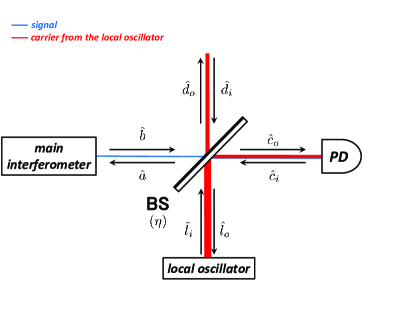
Figure 1: Configuration of the interferometer for the simple homodyne detection. The notations of the quadratures $\hat{a}$, $\hat{b}$, $\hat{c}_{o}$, $\hat{c}_{i}$, $\hat{d}_{o}$, $\hat{d}_{i}$, $\hat{l}_{o}$, and $\hat{l}_{i}$ are also given in this figure.

The output electric field $\hat{E}_{b}$ from the main interferometer is given by

$$\hat{E}_{b}(t)=\int_{0}^{+\infty}\sqrt{\frac{2\pi\hbar|\omega|}{{\cal A}c}}\left(\hat{b}(\omega)e^{-i\omega t}+\hat{b}^{\dagger}(\omega)e^{+i\omega t}\right)\frac{d\omega}{2\pi}$$ (9)

and the electric field from the local oscillator is given by

$$\hat{E}_{l_{i}}(t)=\int_{0}^{+\infty}\sqrt{\frac{2\pi\hbar|\omega|}{{\cal A}c}}\left(\hat{l}_{i}(\omega)e^{-i\omega t}+\hat{l}_{i}^{\dagger}(\omega)e^{+i\omega t}\right)\frac{d\omega}{2\pi}.$$ (10)

Furthermore, the electric field to be detected through the photodetector is given by

$$\hat{E}_{c_{o}}(t)=\int_{0}^{+\infty}\sqrt{\frac{2\pi\hbar|\omega|}{{\cal A}c}}\left(\hat{c}_{o}(\omega)e^{-i\omega t}+\hat{c}_{o}^{\dagger}(\omega)e^{+i\omega t}\right)\frac{d\omega}{2\pi}.$$ (11)

At the beam splitter, the signal electric field $\hat{E}_{b}(t)$ and the electric field $\hat{E}_{l_{i}}(t)$ are mixed and the beam splitter output the electric field $\hat{E}_{c_{o}}(t)$ to the one of the ports. These fields are related by the relation

$$\hat{E}_{c_{o}}(t)=\sqrt{\eta}\hat{E}_{b}(t)+\sqrt{1-\eta}\hat{E}_{l_{i}}(t).$$ (12)

This relation is given in terms of the quadrature relation as

$$\hat{c}_{o}(\omega)=\sqrt{\eta}\hat{b}(\omega)+\sqrt{1-\eta}\hat{l}_{i}(\omega).$$ (13)

Here, we assign the states for the independent electric field described in Fig. 1. As mentioned above, the electric field from the local oscillator is in the coherent state (8). In addition to this state, the electric fields associated with the quadratures $\hat{d}_{i}$ and $\hat{c}_{i}$ are injected into the beam splitter. In this paper, we regard that the electric fields associated with the quadratures $\hat{d}_{i}$ and $\hat{c}_{i}$ are in their vacua, respectively. The junction condition for the electric fields at the beam splitter is given by

$$\hat{E}_{a}(t)=\sqrt{\eta}\hat{E}_{c_{i}}(t)-\sqrt{1-\eta}\hat{E}_{d_{i}}(t).$$ (14)

In terms of quadratures, this relation is given by

$$\hat{a}(\omega)=\sqrt{\eta}\hat{c}_{i}(\omega)-\sqrt{1-\eta}\hat{d}_{i}(\omega).$$ (15)

Due to this relation (15), the state associated with the quadrature $\hat{a}$ is described by the vacuum states for the quadratures $\hat{d}_{i}$ and $\hat{c}_{i}$.

Usually, the state associated with the quadrature $\hat{b}$ depends on the state of the input field $\hat{E}_{a}$ into the main interferometer and the other optical fields which inject to the main interferometer H.J.Kimble-Y.Levin-A.B.Matsko-K.S.Thorne-S.P.Vyatchanin-2001 ; H.Miao-PhDthesis-2010 . Furthermore, in this paper, we consider the situation where the output electric field $\hat{E}_{b}$ includes the information of classical forces as in Eq. (2) and this information are measured through the expectation value of the operator $\hat{b}$.

To evaluate the expectation value of the quadrature $\hat{b}$, we have to specify the state of the total system. Here, we assume that this state of the total system is given by

$$|\Psi\rangle=|\gamma\rangle_{l_{i}}\otimes|0\rangle_{c_{i}}\otimes|0\rangle_{d_{i}}\otimes|\psi\rangle_{\text{main}},$$ (16)

where the state $|\psi\rangle_{\text{main}}$ is the state for the electric fields associated with the main interferometer, which is independent of the states $|\gamma\rangle_{l_{i}}$, $|0\rangle_{c_{i}}$, and $|0\rangle_{d_{i}}$. As noted above, the output quadrature $\hat{b}$ may depends on the input quadrature $\hat{a}$ and this input quadrature $\hat{a}$ is related to the quadratures $\hat{c}_{i}$ and $\hat{d}_{i}$ through Eq. (15). Therefore, strictly speaking, the expectation value of the quadrature $\hat{b}$ means that

$$\langle\hat{b}\rangle=\langle\psi|_{\text{main}}\otimes\langle 0|_{d_{i}}\otimes\langle 0|_{c_{i}}\hat{b}|0\rangle_{c_{i}}\otimes|0\rangle_{d_{i}}\otimes|\psi\rangle_{\text{main}},$$ (17)

but we denote simply

$$\langle\hat{b}\rangle:=\langle\Psi|\hat{b}|\Psi\rangle.$$ (18)

PD in Fig. 1 detects the photon number of the electric field associated with the annihilation operator $\hat{c}_{o}$. So, we evaluate the expectation value of the photon number operator $\hat{n}_{c_{o}}(\omega):=\hat{c}_{o}^{\dagger}(\omega)\hat{c}_{o}(\omega)$. From the condition at the beam splitter, we obtain

$$\hat{n}_{c_{o}}(\omega)=\left(\sqrt{\eta}\hat{b}^{\dagger}(\omega)+\sqrt{1-\eta}\hat{l}_{i}^{\dagger}(\omega)\right)\left(\sqrt{\eta}\hat{b}(\omega)+\sqrt{1-\eta}\hat{l}_{i}(\omega)\right).$$ (19)

Through the definition of the coherent state (7), the expectation value for this number operator (19) under the state (16) for the total system is given by

$$\langle\hat{n}_{c_{o}}(\omega)\rangle := \langle\Psi|\hat{n}_{c_{o}}(\omega)|\Psi\rangle$$ (20)

$$= \eta\left\langle\hat{n}_{b}(\omega)\right\rangle+(1-\eta)\left|\gamma(\omega)\right|^{2}+\sqrt{\eta(1-\eta)}\left\langle\gamma^{*}(\omega)\hat{b}(\omega)+\gamma(\omega)\hat{b}^{\dagger}(\omega)\right\rangle,$$ (21)

where we defined

$$\left\langle\hat{n}_{b}(\omega)\right\rangle=\left\langle\hat{b}^{\dagger}(\omega)\hat{b}(\omega)\right\rangle:=\langle\Psi|\hat{b}^{\dagger}(\omega)\hat{b}(\omega)|\Psi\rangle,$$ (22)

$$\left\langle\gamma^{*}(\omega)\hat{b}(\omega)+\gamma(\omega)\hat{b}^{\dagger}(\omega)\right\rangle:=\langle\Psi|\left(\gamma^{*}(\omega)\hat{b}(\omega)+\gamma(\omega)\hat{b}^{\dagger}(\omega)\right)|\Psi\rangle.$$ (23)

As we assumed above, $\gamma(\omega)$ is a known complex function of $\omega$. Therefore, we can eliminate the term $(1-\eta)|\gamma(\omega)|^{2}$ from the expectation value $\langle\hat{n}_{c_{o}}(\omega)\rangle$, which is the dominant term in Eq. (21) in the situation where the absolute value of $\gamma(\omega)$ is very large. In the same situation, we can neglect the first term $\eta\left\langle\hat{n}_{b}(\omega)\right\rangle$ from the expectation value (21). Then, we can measure the expectation value of the linear combination $\gamma^{*}(\omega)\hat{b}(\omega)$ $+$ $\gamma(\omega)\hat{b}^{\dagger}(\omega)$ of the annihilation- and creation operators for the output field as the subdominant contribution. This is the simple homodyne detection in Fig. 1. We note that the large $\gamma(\omega)$ is essential in this simple homodyne detection.

II.3 Balanced homodyne detection

The optical configuration of the balanced homodyne detection is almost similar to the simple homodyne detection depicted in Fig. 1, but the difference is in the additional photon detection through the photodetector D2 in Fig. 2 at another port of the beam splitter.

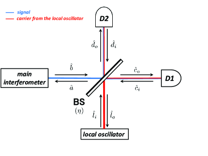
Figure 2: Configuration of the interferometer for the balanced homodyne detection. This notation of the quadratures are same as those in Fig. 1.

To discuss the output of the balanced homodyne detection, we consider the photon number operators detected by the photodetectors D1 and D2 in Fig. 2, respectively. At the photodetector D1, we count the photon number which expressed the operator (19) in Sec. II.2. Since the total state of the system is same as the state (16) in the case of the simple homodyne detector, the expectation value of the operator (19) is also given by Eq. (21) in Sec. II.2. On the other hand, we also detect the photon number through the photodetector D2 in the balanced homodyne detection.

Following the notation of quadratures depicted in Fig. 2, the photon number operator which is detected at the photodetector D2 is given by $\hat{n}_{d_{o}}(\omega):=\hat{d}_{o}^{\dagger}(\omega)\hat{d}_{o}(\omega)$. The output electric field $\hat{E}_{d_{o}}(t)$ is produced through the mixing of the signal electric field $\hat{E}_{b}(t)$ and the electric field $\hat{E}_{l_{i}}(t)$ from the local oscillator at the beam splitter as

$$\hat{E}_{d_{o}}(t)=\sqrt{\eta}\hat{E}_{b}(t)-\sqrt{1-\eta}\hat{E}_{l_{i}}(t).$$ (24)

This relation gives the quadrature relation as

$$\hat{d}_{o}(\omega)=\sqrt{\eta}\hat{b}(\omega)-\sqrt{1-\eta}\hat{l}_{i}(\omega).$$ (25)

Then, the photon number operator $\hat{n}_{d_{o}}(\omega)$ is given by

$$\hat{n}_{d_{o}}(\omega)=\left(\sqrt{\eta}\hat{l}_{i}(\omega)-\sqrt{1-\eta}\hat{b}(\omega)\right)^{\dagger}\left(\sqrt{\eta}\hat{l}_{i}(\omega)-\sqrt{1-\eta}\hat{b}(\omega)\right).$$ (26)

The expectation value of the operator $\hat{n}_{d_{o}}(\omega)$ in the state (16) is given by

$$\langle\hat{n}_{d_{o}}(\omega)\rangle := \langle\Psi|\hat{n}_{d_{o}}(\omega)|\Psi\rangle$$ (27)

$$= (1-\eta)\langle\hat{n}_{b}(\omega)\rangle+\eta|\gamma(\omega)|^{2}-\sqrt{\eta(1-\eta)}\left\langle\gamma^{*}(\omega)\hat{b}(\omega)+\gamma(\omega)\hat{b}^{\dagger}(\omega)\right\rangle,$$

where we used Eqs. (22) and (23).

Taking the linear combination of Eqs. (21) and (27), we obtain

$$(1-\eta)\langle\hat{n}_{c_{o}}(\omega)\rangle-\eta\langle\hat{n}_{d_{o}}(\omega)\rangle$$ (28)

$$= \left(1-2\eta\right)\left|\gamma(\omega)\right|^{2}+\sqrt{\eta(1-\eta)}\left\langle\gamma^{*}(\omega)\hat{b}(\omega)+\gamma(\omega)\hat{b}^{\dagger}(\omega)\right\rangle.$$

Since $\gamma(\omega)$ is a known complex function, we can always subtract the first term in Eq. (28) from the output signal. Then, we can unambiguously measure the linear combination of the quadrature $\hat{b}(\omega)$ and $\hat{b}^{\dagger}(\omega)$ as

$$\left\langle\gamma^{*}(\omega)\hat{b}(\omega)+\gamma(\omega)\hat{b}^{\dagger}(\omega)\right\rangle = \frac{(1-\eta)\langle\hat{n}_{c_{o}}(\omega)\rangle-\eta\langle\hat{n}_{d_{o}}(\omega)\rangle-\left(1-2\eta\right)\left|\gamma(\omega)\right|^{2}}{\sqrt{\eta(1-\eta)}}.$$ (29)

This is the balanced homodyne detection.

The right-hand side of Eq. (29) is also regarded as the expectation value of the operator $\hat{s}(\omega)$ defined by

$$\hat{s}(\omega) := \frac{1}{(\eta(1-\eta))^{1/2}}\left\{(1-\eta)\hat{n}_{c_{o}}(\omega)-\eta\hat{n}_{d_{o}}(\omega)-\left(1-2\eta\right)\left|\gamma(\omega)\right|^{2}\right\},$$ (30)

$$= \hat{l}_{i}^{\dagger}(\omega)\hat{b}(\omega)+\hat{b}^{\dagger}(\omega)\hat{l}_{i}(\omega)+\frac{1-2\eta}{\sqrt{\eta(1-\eta)}}\left(\hat{l}_{i}^{\dagger}(\omega)\hat{l}_{i}(\omega)-\left|\gamma(\omega)\right|^{2}\right),$$ (31)

where we used Eqs. (19) and (26). Actually, the expectation value of the operator (31) under the state (16) yields the left-hand side of Eq. (29). Here, we note that the operator $\hat{s}(\omega)$ is a self-adjoint operator due to the fact that the photon number operators are self-adjoint and $\hat{s}(\omega)$ is given by the linear combination of these number operators with real coefficients. Therefore, the expectation value $\langle\hat{s}(\omega)\rangle$ of the operator $\hat{s}(\omega)$ must be real as seen in the right-hand side Eq. (29).

III Balanced homodyne detection in the two-photon formulation

In the community of gravitational-wave detections, the two-photon formulation C.M.Caves-B.L.Schumaker-1985 is used under the condition $\omega_{0}\gg\Omega$, where $\omega_{0}$ is the frequency of the classical carrier field and $\Omega$ is its sideband frequency. In Sec. III.1, we introduce the amplitude quadrature $\hat{b}_{1}$ and phase-quadratures $\hat{b}_{2}$ in Eq. (1). In Sec. III.2, we examine whether or not we can measure the combination (1) through the simple application of the balanced homodyne detection reviewed in Sec. II.3 and show that we cannot measure the expectation value of the combination $\hat{b}_{\theta}$ in Eq. (1) by the simple application of the balanced homodyne detection in Sec. II.3. In Sec. III.3, we describe some remarks of the examination in Sec. III.2.

III.1 Amplitude quadrature and phase quadrature

Keeping in our mind the above situation $\omega_{0}\gg\Omega$ of the two-photon formulation, we introduce variables $\hat{b}_{\pm}$, $\hat{l}_{\pm}$, and $\gamma_{\pm}$ as

$$\hat{b}_{\pm}(\Omega):=\hat{b}(\omega_{0}\pm\Omega),\quad\hat{l}_{i\pm}(\Omega):=\hat{l}_{i}(\omega_{0}\pm\Omega),\quad\gamma_{\pm}(\Omega):=\gamma(\omega_{0}\pm\Omega).$$ (32)

In this situation, the operator (31) of the homodyne detection is given by

$$\hat{s}_{\pm} = \hat{l}_{i\pm}^{\dagger}\hat{b}_{\pm}+\hat{b}_{\pm}^{\dagger}\hat{l}_{i\pm}+\frac{1-2\eta}{\sqrt{\eta(1-\eta)}}\left(\hat{l}_{i\pm}^{\dagger}\hat{l}_{i\pm}-\left|\gamma_{\pm}\right|^{2}\right).$$ (33)

Furthermore, we introduce the amplitude and phase quadratures as

$$\hat{b}_{1}:=\frac{1}{\sqrt{2}}\left(\hat{b}_{+}+\hat{b}_{-}^{\dagger}\right),\quad\hat{b}_{2}:=\frac{1}{\sqrt{2}i}\left(\hat{b}_{+}-\hat{b}_{-}^{\dagger}\right).$$ (34)

Under the existence of the classical carrier field which proportional to $\cos\omega_{0}t$, $\bar{b}_{1}$ and $\hat{b}_{2}$ are regarded as the quadratures for the amplitude fluctuations and the phase fluctuations, respectively. The definitions (34) are equivalent to

$$\hat{b}_{+}:=\frac{1}{\sqrt{2}}\left(\hat{b}_{1}+i\hat{b}_{2}\right),\quad\hat{b}_{-}:=\frac{1}{\sqrt{2}}\left(\hat{b}_{1}^{\dagger}+i\hat{b}_{2}^{\dagger}\right).$$ (35)

As mentioned above, the aim of this section is to examine whether or not the expectation-value measurement of the quadrature (1) with the homodyne angle $\theta$ is possible through the simple application of the balanced homodyne detection described in Sec. II.3. To carry out this examination, we have to consider the expectation values of the operator $\hat{s}_{\pm}$ defined by Eq. (33) as

$$\left\langle\hat{s}_{+}\right\rangle=\left\langle\gamma_{+}^{*}\hat{b}_{+}+\hat{b}_{+}^{\dagger}\gamma_{+}\right\rangle,\quad\left\langle\hat{s}_{-}\right\rangle=\left\langle\gamma_{-}^{*}\hat{b}_{-}+\hat{b}_{-}^{\dagger}\gamma_{-}\right\rangle.$$ (36)

Substituting Eqs. (35) into Eqs. (36) and taking linear combination of $\langle\hat{s}_{+}\rangle$ and $\langle\hat{s}_{-}\rangle$, we obtain

$$\alpha\left\langle\hat{s}_{+}\right\rangle+\beta\left\langle\hat{s}_{-}\right\rangle = \frac{1}{\sqrt{2}}\left\langle\left(\alpha\gamma_{+}^{*}+\beta\gamma_{-}\right)\hat{b}_{1}+i\left(\alpha\gamma_{+}^{*}-\beta\gamma_{-}\right)\hat{b}_{2}\right.$$ (37)

$$\quad\quad\quad\quad\left.+\left(\alpha\gamma_{+}+\beta\gamma_{-}^{*}\right)\hat{b}_{1}^{\dagger}+i\left(-\alpha\gamma_{+}+\beta\gamma_{-}^{*}\right)\hat{b}_{2}^{\dagger}\right\rangle.$$

The linear combination (37) yields the possible output signal by choosing the complex parameter $\alpha$, $\beta$, and $\gamma_{\pm}$ which are completely controllable.

III.2 Can we measure the expectation value of $\hat{b}_{\theta}$ by the simple application of the balanced homodyne detection?

To examine the problem whether or not we can measure the expectation value of the linear combination defined by Eq. (1) through an appropriate choice of $\alpha$, $\beta$, and $\gamma_{\pm}$, in this subsection, we consider the cases where the output signal (37) yields the linear combination of the two quadratures among $\hat{b}_{1}$, $\hat{b}_{1}^{\dagger}$, $\hat{b}_{2}$, and $\hat{b}_{2}^{\dagger}$. To do this, we treat following six cases.

III.2.1 Linear combination of $\hat{b}_{1}$ and $\hat{b}_{2}$

Here, we check whether or not the linear combination (37) is expressed by a linear combination of $\hat{b}_{1}$ and $\hat{b}_{2}$, which is already given in Ref. K.Nakamura-M.-K.Fujimoto-2017b . This should be accomplished by the equation of the matrix form:

$$\left(\begin{array}[]{cc}\gamma_{+}&\gamma_{-}^{*}\\ -\gamma_{+}&\gamma_{-}^{*}\end{array}\right)\left(\begin{array}[]{c}\alpha\\ \beta\end{array}\right)=\left(\begin{array}[]{c}0\\ 0\end{array}\right).$$ (44)

If a nontrivial solution $(\alpha,\beta)\neq(0,0)$ to Eq. (44) exists, the determinant of the matrix in Eq. (44) should vanish, i.e., $2\gamma_{+}\gamma_{-}^{*}=0$. This implies that $\gamma_{+}=0$ or $\gamma_{-}=0$. These cases are meaningless as balanced homodyne detections. This fact implies that the linear combination of $\langle\hat{s}_{\pm}\rangle$ does not give expectation values of the linear combination of $\hat{b}_{1}$ and $\hat{b}_{2}$, by itself. This result directly means that the output signal (37) never yields the expectation value of the operator (1).

III.2.2 Linear combination of $\hat{b}_{1}$ and $\hat{b}_{1}^{\dagger}$

Here, we check whether or not Eq. (37) yields a linear combination of $\hat{b}_{1}$ and $\hat{b}_{1}^{\dagger}$. This situation should be accomplished by the equations of the matrix form:

$$\left(\begin{array}[]{cc}\gamma_{+}^{*}&-\gamma_{-}\\ -\gamma_{+}&\gamma_{-}^{*}\end{array}\right)\left(\begin{array}[]{c}\alpha\\ \beta\end{array}\right)=\left(\begin{array}[]{c}0\\ 0\end{array}\right).$$ (51)

If a nontrivial solution $(\alpha,\beta)\neq(0,0)$ to Eq. (51) exists, the determinant of the matrix in Eq. (51) should vanish : $(\gamma_{+}\gamma_{-})^{*}=\gamma_{+}\gamma_{-}$, i.e., $\gamma_{+}\gamma_{-}$ is real and we may choose so that

$$\gamma_{+}=|\gamma_{+}|e^{i\theta},\quad\gamma_{-}=|\gamma_{-}|e^{-i\theta}.$$ (52)

Substituting these expressions into Eqs. (51), we obtain

$$\beta=\frac{|\gamma_{+}|}{|\gamma_{-}|}\alpha.$$ (53)

Furthermore, substituting Eqs. (52) and (53) into Eq. (37) , we obtain

$$\frac{\left\langle\hat{s}_{+}\right\rangle}{|\gamma_{+}|}+\frac{\left\langle\hat{s}_{-}\right\rangle}{|\gamma_{-}|}=\sqrt{2}\left\langle\hat{b}_{1}e^{-i\theta}+\hat{b}_{1}^{\dagger}e^{+i\theta}\right\rangle.$$ (54)

III.2.3 Linear combination of $\hat{b}_{1}$ and $\hat{b}_{2}^{\dagger}$

Here, we check whether or not Eq. (37) is expressed the linear combination of $\hat{b}_{1}$ and $\hat{b}_{2}^{\dagger}$. In this case, the following conditions should be satisfied:

$$\left(\begin{array}[]{cc}\gamma_{+}^{*}&-\gamma_{-}\\ \gamma_{+}&\gamma_{-}^{*}\end{array}\right)\left(\begin{array}[]{c}\alpha\\ \beta\end{array}\right)=\left(\begin{array}[]{c}0\\ 0\end{array}\right).$$ (61)

The condition for the existence of the nontrivial solution $(\alpha,\beta)\neq(0,0)$ to Eq. (61) is $(\gamma_{+}\gamma_{-})^{*}=-\gamma_{+}\gamma_{-}$, i.e., $\gamma_{+}\gamma_{-}$ is purely imaginary. Therefore, we may choose $\gamma_{\pm}$ as

$$\gamma_{+}=|\gamma_{+}|e^{+i\theta},\quad\gamma_{-}=i|\gamma_{-}|e^{-i\theta}.$$ (62)

Substituting Eq. (62) into Eq. (61), we obtain the relation

$$\beta=-i\frac{|\gamma_{+}|}{|\gamma_{-}|}\alpha$$ (63)

Furthermore, substituting Eqs. (62) and (63) into Eq. (37), we obtain

$$\frac{\left\langle\hat{s}_{+}\right\rangle}{|\gamma_{+}|}-i\frac{\left\langle\hat{s}_{-}\right\rangle}{|\gamma_{-}|}=\sqrt{2}\left\langle e^{-i\theta}\hat{b}_{1}-ie^{+i\theta}\hat{b}_{2}^{\dagger}\right\rangle.$$ (64)

III.2.4 Linear combination of $\hat{b}_{1}^{\dagger}$ and $\hat{b}_{2}$

Here, we check whether or not Eq. (37) yields the linear combination of $\hat{b}_{1}^{\dagger}$ and $\hat{b}_{2}$. This should be accomplished by the equation of the matrix form:

$$\left(\begin{array}[]{cc}\gamma_{+}^{*}&\gamma_{-}\\ -\gamma_{+}&\gamma_{-}^{*}\end{array}\right)\left(\begin{array}[]{c}\alpha\\ \beta\end{array}\right)=\left(\begin{array}[]{c}0\\ 0\end{array}\right).$$ (71)

The existence of the nontrivial solution $(\alpha,\beta)\neq(0,0)$ to Eq. (71) is guaranteed by the vanishing condition of the determinant of the matrix in Eq. (71). This condition is given by $(\gamma_{+}\gamma_{-})^{*}=-\gamma_{+}\gamma_{-}$, i.e., $\gamma_{+}\gamma_{-}$ is purely imaginary and we may choose $\gamma_{\pm}$ as

$$\gamma_{+}=|\gamma_{+}|e^{+i\theta},\quad\gamma_{-}=i|\gamma_{-}|e^{-i\theta}.$$ (72)

Substituting Eq. (72) into Eq. (71), we obtain

$$\beta=i\frac{|\gamma_{+}|}{|\gamma_{-}|}\alpha.$$ (73)

Further, through Eqs. (72) and (73), the linear combination (37) is given by

$$\frac{\left\langle\hat{s}_{+}\right\rangle}{|\gamma_{+}|}+i\frac{\left\langle\hat{s}_{-}\right\rangle}{|\gamma_{-}|}=\sqrt{2}\left\langle ie^{-i\theta}\hat{b}_{2}+e^{+i\theta}\hat{b}_{1}^{\dagger}\right\rangle.$$ (74)

III.2.5 Linear combination of $\hat{b}_{1}^{\dagger}$ and $\hat{b}_{2}^{\dagger}$

Here, we examine whether or not the linear combination (37) is given by a linear combination of $\hat{b}_{1}^{\dagger}$ and $\hat{b}_{2}^{\dagger}$. This case is accomplished by the equation of the matrix form

$$\left(\begin{array}[]{cc}\gamma_{+}^{*}&\gamma_{-}\\ \gamma_{+}^{*}&-\gamma_{-}\end{array}\right)\left(\begin{array}[]{c}\alpha\\ \beta\end{array}\right)=\left(\begin{array}[]{c}0\\ 0\end{array}\right).$$ (81)

The existence of the nontrivial solution $(\alpha,\beta)\neq(0,0)$ to Eq. (81) is given by $\gamma_{+}^{*}\gamma_{-}$, which implies that $\gamma_{+}=0$ or $\gamma_{-}=0$. These are meaningless as balanced homodyne detections as in the case in Sec. III.2.1. This fact implies that the linear combination (37) does not give expectation values of the linear combination of $\hat{b}_{1}^{\dagger}$ and $\hat{b}_{2}^{\dagger}$. This is consistent with the result in Sec. III.2.1.

III.2.6 Linear combination of $\hat{b}_{2}$ and $\hat{b}_{2}^{\dagger}$

Finally, we check whether the linear combination (37) is expressed by a linear combination of $\hat{b}_{2}$ and $\hat{b}_{2}^{\dagger}$, or not. This case is accomplished by the equation of the matrix form

$$\left(\begin{array}[]{cc}\gamma_{+}^{*}&\gamma_{-}\\ \gamma_{+}&\gamma_{-}^{*}\end{array}\right)\left(\begin{array}[]{c}\alpha\\ \beta\end{array}\right)=\left(\begin{array}[]{c}0\\ 0\end{array}\right).$$ (88)

The existence of nontrivial solutions $(\alpha,\beta)\neq(0,0)$ to Eq. (88) is guaranteed by the vanishing determinant of the matrix in Eq. (88). This condition is given by $(\gamma_{+}\gamma_{-})^{*}=\gamma_{-}\gamma_{+}$, which means that $\gamma_{+}\gamma_{-}$ is real. Therefore, we may choose $\gamma_{\pm}$ so that

$$\gamma_{+}=|\gamma_{+}|e^{+i\theta},\quad\gamma_{-}=|\gamma_{-}|e^{-i\theta}.$$ (89)

Through Eqs. (89) and (88), we obtain

$$\beta=-\alpha\frac{|\gamma_{+}|}{|\gamma_{-}|}.$$ (90)

Substituting Eqs. (89) and (90) into Eq. (37), we obtain

$$\frac{\left\langle\hat{s}_{+}\right\rangle}{|\gamma_{+}|}-\frac{\left\langle\hat{s}_{-}\right\rangle}{|\gamma_{-}|}=\sqrt{2}i\left\langle e^{-i\theta}\hat{b}_{2}-e^{+i\theta}\hat{b}_{2}^{\dagger}\right\rangle.$$ (91)

III.3 Remarks

Combination	Possible?		$\gamma_{+}$		$\gamma_{-}$		$\alpha$-$\beta$ relation
$\displaystyle\hat{b}_{1}$ and $\displaystyle\hat{b}_{2}$	$\displaystyle\times$		—		—		—
$\displaystyle\hat{b}_{1}$ and $\displaystyle\hat{b}_{1}^{\dagger}$	$\displaystyle\bigcirc$		$\displaystyle|\gamma_{+}|e^{+i\theta}$		$\displaystyle|\gamma_{-}|e^{-i\theta}$		$\displaystyle\beta=\frac{|\gamma_{+}|}{|\gamma_{-}|}\alpha$
$\displaystyle\hat{b}_{1}$ and $\displaystyle\hat{b}_{2}^{\dagger}$	$\displaystyle\bigcirc$		$\displaystyle|\gamma_{+}|e^{+i\theta}$		$\displaystyle i|\gamma_{-}|e^{-i\theta}$		$\displaystyle\beta=-i\frac{|\gamma_{+}|}{|\gamma_{-}|}\alpha$
$\displaystyle\hat{b}_{1}^{\dagger}$ and $\displaystyle\hat{b}_{2}$	$\displaystyle\bigcirc$		$\displaystyle|\gamma_{+}|e^{+i\theta}$		$\displaystyle i|\gamma_{-}|e^{-i\theta}$		$\displaystyle\beta=+i\frac{|\gamma_{+}|}{|\gamma_{-}|}\alpha$
$\displaystyle\hat{b}_{1}^{\dagger}$ and $\displaystyle\hat{b}_{2}^{\dagger}$	$\displaystyle\times$		—		—		—
$\displaystyle\hat{b}_{2}$ and $\displaystyle\hat{b}_{2}^{\dagger}$	$\displaystyle\bigcirc$		$\displaystyle|\gamma_{+}|e^{+i\theta}$		$\displaystyle|\gamma_{-}|e^{-i\theta}$		$\displaystyle\beta=-\frac{|\gamma_{+}|}{|\gamma_{-}|}\alpha$

Table 1: Summary of the problem whether or not the linear combination (37) can be reduced to the linear combination of two quadratures. In this table, the value of $\gamma_{+}$ is always arbitrary expect for the non-vanishing condition $\gamma_{+}\neq 0$ but the corresponding choice of $\gamma_{-}$ is nontrivial. This table indicates that the relative phase of $\gamma_{\pm}$ is important for the reduction of Eq. (37) to the linear combination of two quadratures.

We have shown that we cannot measure the expectation value of any linear combination of $\hat{b}_{1}$ and $\hat{b}_{2}$ in Sec. III.2.1 through the simple application of the balanced homodyne detection. Similarly, we cannot directly measure the linear combination of $\hat{b}_{1}^{\dagger}$ and $\hat{b}_{2}^{\dagger}$ as we have seen in Sec. III.2.5. These two cases are consistent with each other. These also indicates that we cannot measure the expectation value of the operator $\hat{b}_{\theta}$ through the simple application of the balanced homodyne detection reviewed in Sec. II.3.

On the other hand, as seen in Sec. III.2.2, we can measure the expectation value of the linear combination of $\hat{b}_{1}$ and $\hat{b}_{1}^{\dagger}$ through the linear combination of the expectation values $\langle\hat{s}_{\pm}\rangle$ with real coefficients $\alpha$ and $\beta$ as seen in Eqs. (53) and (54). To accomplish this, the phase of the complex amplitude $\gamma_{\pm}$ for the coherent state from the local oscillator should be opposite as seen in Eq. (52). This is an important requirement for the coherent state from the local oscillator.

Similarly, as seen in Sec. III.2.6, we can also measure the expectation value of the linear combination of $\hat{b}_{2}$ and $\hat{b}_{2}^{\dagger}$ through the linear combination of the expectation values $\langle\hat{s}_{\pm}\rangle$ with real coefficients $\alpha$ and $\beta$ as seen in Eqs. (90) and (54). To accomplish this, the phase of the complex amplitude $\gamma_{\pm}$ for the coherent state from the local oscillator should be opposite as seen in Eq. (89). As in the case of Sec. III.2.2, the phase condition for the local oscillator also is crucial.

The results of the above arguments in Sec. III.2 is summarized in Table 1. In addition to the choice of the relation of the coefficients $\alpha$ and $\beta$, Table 1 indicates that the relative phase of $\gamma_{\pm}$ of the local oscillator is important for the reduction of Eq. (37) to the linear combination of two quadratures from $\hat{b}_{1}$, $\hat{b}_{2}$, $\hat{b}_{1}^{\dagger}$, and $\hat{b}_{2}^{\dagger}$.

Two cases in Sec. III.2.2 and Sec. III.2.6 are the cases of the real coefficients $\alpha$ and $\beta$. Since the operators $\hat{s}_{\pm}$ are self-adjoint operators, the resulting operators are also self-adjoint. Interestingly, the complex coefficients $\alpha$ and $\beta$ of the linear combination of $\langle\hat{s}_{\pm}\rangle$ is also possible as seen in Sec. III.2.3 and in Sec. III.2.4. In these cases, the results are no longer self-adjoint operators in spite that the operators $\hat{s}_{\pm}$ are self-adjoint. Therefore, we can calculate an expectation value of non-self-adjoint operators from the expectation values of the self-adjoint operators which can be directly calculable from the expectation values of photon number operators in the balanced homodyne detection reviewed in Sec. II.3.

Finally, we also note that in any possible cases in Sec. III.2, the phase control of the upper- and lower-sidebands is necessary. Namely, from the local oscillator, we have to introduce the coherent state with the complex amplitudes $\gamma_{\pm}=\gamma(\omega_{0}\pm\Omega)$ for upper- and lower-sideband have the opposite phase as in Eqs. (52), (62), (72), and (89). Before these important requirements for the phase of $\gamma_{\pm}$, $\gamma_{\pm}$ must have their non-vanishing support at the frequency $\omega_{0}\pm\Omega$. These requirements for the coherent state from the local oscillator are also important results from our examination in this section.

IV Double balanced homodyne detection

Through the understanding of the balanced homodyne detections based on the examinations in Sec. III, we propose the “double balanced homodyne detection” which enable us to measure the expectation values for the photon annihilation and creation operators themselves. In Sec. IV.1, we describe our theoretical proposal of a double balanced homodyne detection. In Sec. IV.2, we propose a realization of our double balanced homodyne detection through the interferometer setup. In Sec. IV.3, we discuss the commutation relations between each electric field in the interferometer with the input field to the main interferometer. In Sec. IV.4, we show the double balanced homodyne detection through our interferometer setup enable us to measure the expectation values of the annihilation and creation operators for the output quadrature from the main interferometer. Finally, in Sec. IV.5, we show that the expectation value of the operator (1) of the output quadrature from the main interferometer can be measured through our interferometer setup. In this section, we assume $|\gamma_{\pm}|=:|\gamma|$, for simplicity. The generalization to the case where $|\gamma_{+}|\neq|\gamma_{-}|$ is always possible and straightforward as seen in Appendix A.

IV.1 Theoretical proposal

In this subsection, we describe our theoretical proposal of the double balanced homodyne detection. In Sec. IV.1.1, we describe how to realize the expectation values of $\hat{b}_{1}$, $\hat{b}_{1}^{\dagger}$, $\hat{b}_{2}$, or $\hat{b}_{2}^{\dagger}$ in the calculations on papers. The idea in Sec. IV.1.1 is extended in Sec. IV.1.2 to the measurement of the linear combination (1).

IV.1.1 Expectation values of $\hat{b}_{1}$, $\hat{b}_{1}^{\dagger}$, $\hat{b}_{2}$, and $\hat{b}_{2}^{\dagger}$

Here again, we consider the case in Sec. III.2.2. In this case, the linear combination (37) is given by

$$\frac{1}{\sqrt{2}|\gamma|}\left(\left\langle\hat{s}_{+}\right\rangle+\left\langle\hat{s}_{-}\right\rangle\right)=\langle\hat{b}_{1}\rangle e^{-i\theta}+\langle\hat{b}_{1}^{\dagger}\rangle e^{+i\theta}.$$ (92)

Since the complex amplitude $\gamma$ including its phase is completely controllable, we may choose $\theta=0$ or $\theta=\pi/2$, for example. In the cases where $\theta=0$ and $\theta=\pi/2$, Eq. (92) are given by

$$\left.\frac{1}{\sqrt{2}|\gamma|}\left(\left\langle\hat{s}_{+}\right\rangle+\left\langle\hat{s}_{-}\right\rangle\right)\right|_{\theta=0}=\langle\hat{b}_{1}\rangle+\langle\hat{b}_{1}^{\dagger}\rangle,$$ (93)

$$\left.\frac{1}{\sqrt{2}|\gamma|}\left(\left\langle\hat{s}_{+}\right\rangle+\left\langle\hat{s}_{-}\right\rangle\right)\right|_{\theta=\pi/2}=-i\langle\hat{b}_{1}\rangle+i\langle\hat{b}_{1}^{\dagger}\rangle.$$ (94)

If we can produce the results Eqs. (93) and (94) as the measurement results at the same time, we can calculate

$$\frac{1}{2\sqrt{2}|\gamma|}\left\{\left.\left(\left\langle\hat{s}_{+}\right\rangle+\left\langle\hat{s}_{-}\right\rangle\right)\right|_{\theta=0}+\left.i\left(\left\langle\hat{s}_{+}\right\rangle+\left\langle\hat{s}_{-}\right\rangle\right)\right|_{\theta=\pi/2}\right\} = \langle\hat{b}_{1}\rangle,$$ (95)

$$\frac{1}{2\sqrt{2}|\gamma|}\left\{\left.\left(\left\langle\hat{s}_{+}\right\rangle+\left\langle\hat{s}_{-}\right\rangle\right)\right|_{\theta=0}-\left.i\left(\left\langle\hat{s}_{+}\right\rangle+\left\langle\hat{s}_{-}\right\rangle\right)\right|_{\theta=\pi/2}\right\} = \langle\hat{b}_{1}^{\dagger}\rangle.$$ (96)

Note that $\langle\hat{s}_{\pm}\rangle$ are measured from the photon-number expectation values through the balanced homodyne detection. Since $\gamma$ is controllable, Eq. (95) and (96) imply that the expectation values $\langle\hat{b}_{1}\rangle$ and $\langle\hat{b}_{1}^{\dagger}\rangle$ of the quadrature is indirectly calculable from these measurement, respectively, though the operators $\hat{b}_{1}$ is not self-adjoint operator. This situation is similar to the cases in Sec. III.2.3 and Sec. III.2.4.

Similar analysis is possible even in the case in Sec. III.2.6. The results yield that we can calculate the expectation values of the quadrature $\langle\hat{b}_{2}\rangle$ and $\langle\hat{b}_{2}^{\dagger}\rangle$ from the expectation values $\langle\hat{s}_{\pm}\rangle$ which can be calculated from the expectation values of photon number operators in the balanced homodyne detection. Actually, the result (91) in Sec. III.2.6 is given by

$$\frac{1}{\sqrt{2}i|\gamma|}\left(\langle\hat{s}_{+}\rangle-\langle\hat{s}_{-}\rangle\right)=e^{-i\theta}\langle\hat{b}_{2}\rangle-e^{+i\theta}\langle\hat{b}_{2}^{\dagger}\rangle.$$ (97)

As in the case of Eq. (92), we obtain the expectation values $\langle\hat{b}_{2}\rangle$ and $\langle\hat{b}_{2}^{\dagger}\rangle$ as follows:

$$\frac{1}{2\sqrt{2}|\gamma|}\left\{\left.-i\left(\langle\hat{s}_{+}\rangle-\langle\hat{s}_{-}\rangle\right)\right|_{\theta=0}+\left.\left(\langle\hat{s}_{+}\rangle-\langle\hat{s}_{-}\rangle\right)\right|_{\theta=\pi/2}\right\} = \langle\hat{b}_{2}\rangle,$$ (98)

$$\frac{1}{2\sqrt{2}|\gamma|}\left\{i\left.\left(\langle\hat{s}_{+}\rangle-\langle\hat{s}_{-}\rangle\right)\right|_{\theta=0}+\left.\left(\langle\hat{s}_{+}\rangle-\langle\hat{s}_{-}\rangle\right)\right|_{\theta=\pi/2}\right\} = \langle\hat{b}_{2}^{\dagger}\rangle.$$ (99)

We note that Eq. (99) is important in the gravitational-wave detection, because the phase quadrature $\hat{b}_{2}$ includes gravitational wave signal in many conventional interferometers.

IV.1.2 Expectation value of $\hat{b}_{\theta}=\cos\theta\hat{b}_{1}+\sin\theta\hat{b}_{2}$

Inspecting analyses in the previous section and Appendix A, we introduce the operators $\hat{t}_{\pm}$ which are defined by

$$\hat{t}_{+}:=\frac{1}{\sqrt{2}|\gamma|}\left(\hat{s}_{+}+\hat{s}_{-}\right),\quad\hat{t}_{-}:=\frac{1}{\sqrt{2}i|\gamma|}\left(\hat{s}_{+}-\hat{s}_{-}\right)$$ (100)

to consider the expectation value of the operator $\hat{b}_{\theta}$. We require $\theta_{\pm}=\theta$ as the requirement for the phase of the complex amplitudes $\gamma_{\pm}$ as discussed in Appendix A. In addition, we assumed $|\gamma_{\pm}|=|\gamma|$ for simplicity. We note the operator $\hat{t}_{+}$ is self-adjoint and the operator $\hat{t}_{-}$ is anti-self-adjoint.

From the expressions (33) of the operators $\hat{s}_{\pm}$, we obtain

$$\frac{\hat{s}_{\pm}}{|\gamma|} = \frac{\hat{l}_{i\pm}^{\dagger}}{|\gamma|}\hat{b}_{\pm}+\frac{\hat{l}_{i\pm}}{|\gamma|}\hat{b}_{\pm}^{\dagger}+\frac{1-2\eta}{\eta^{1/2}(1-\eta)^{1/2}}|\gamma|\left(\frac{\hat{l}_{i\pm}^{\dagger}}{|\gamma|}\frac{\hat{l}_{i\pm}}{|\gamma|}-1\right)$$ (101)

and the above operators $\hat{t}_{\pm}$ are given by

$$\hat{t}_{+} = \frac{1}{\sqrt{2}}\left\{\frac{\hat{l}_{i+}^{\dagger}}{|\gamma|}\hat{b}_{+}+\frac{\hat{l}_{i+}}{|\gamma|}\hat{b}_{+}^{\dagger}+\frac{1-2\eta}{\eta^{1/2}(1-\eta)^{1/2}}|\gamma|\left(\frac{\hat{l}_{i+}^{\dagger}}{|\gamma|}\frac{\hat{l}_{i+}}{|\gamma|}-1\right)\right.$$ (102)

$$\quad\quad\quad\left.+\frac{\hat{l}_{i-}^{\dagger}}{|\gamma|}\hat{b}_{-}+\frac{\hat{l}_{i-}}{|\gamma|}\hat{b}_{-}^{\dagger}+\frac{1-2\eta}{\eta^{1/2}(1-\eta)^{1/2}}|\gamma|\left(\frac{\hat{l}_{i-}^{\dagger}}{|\gamma|}\frac{\hat{l}_{i-}}{|\gamma|}-1\right)\right\},$$

and

$$\hat{t}_{-} = \frac{1}{\sqrt{2}i}\left\{\frac{\hat{l}_{i+}^{\dagger}}{|\gamma|}\hat{b}_{+}+\frac{\hat{l}_{i+}}{|\gamma|}\hat{b}_{+}^{\dagger}+\frac{1-2\eta}{\eta^{1/2}(1-\eta)^{1/2}}|\gamma|\left(\frac{\hat{l}_{i+}^{\dagger}}{|\gamma|}\frac{\hat{l}_{i+}}{|\gamma|}-1\right)\right.$$ (103)

$$\quad\quad\quad\left.-\frac{\hat{l}_{i-}^{\dagger}}{|\gamma|}\hat{b}_{-}-\frac{\hat{l}_{i-}}{|\gamma|}\hat{b}_{-}^{\dagger}-\frac{1-2\eta}{\eta^{1/2}(1-\eta)^{1/2}}|\gamma|\left(\frac{\hat{l}_{i-}^{\dagger}}{|\gamma|}\frac{\hat{l}_{i-}}{|\gamma|}-1\right)\right\}.$$

The expectation value of the operators (102) and (103) with the requirement $\theta_{\pm}=\theta$ are given by

$$\left.\left\langle\hat{t}_{+}\right\rangle\right|_{\theta_{\pm}=\theta} = \frac{1}{\sqrt{2}}\left\langle e^{-i\theta}\hat{b}_{+}+e^{+i\theta}\hat{b}_{+}^{\dagger}+e^{-i\theta}\hat{b}_{-}+e^{+i\theta}\hat{b}_{-}^{\dagger}\right\rangle$$ (104)

$$= \left\langle\left(\cos\theta\hat{b}_{1}+\sin\theta\hat{b}_{2}\right)+\left(\cos\theta\hat{b}_{1}+\sin\theta\hat{b}_{2}\right)^{\dagger}\right\rangle,$$ (105)

and

$$\left.\left\langle\hat{t}_{-}\right\rangle\right|_{\theta_{\pm}=\theta} = \frac{1}{\sqrt{2}i}\left\langle e^{-i\theta}\hat{b}_{+}+e^{+i\theta}\hat{b}_{+}^{\dagger}-e^{-i\theta}\hat{b}_{-}-e^{+i\theta}\hat{b}_{-}^{\dagger}\right\rangle$$ (106)

$$= \left\langle\left(-\sin\theta\hat{b}_{1}+\cos\theta\hat{b}_{2}\right)-\left(-\sin\theta\hat{b}_{1}+\cos\theta\hat{b}_{2}\right)^{\dagger}\right\rangle.$$ (107)

Here, we used the fact that the states for the quadratures $\hat{l}_{\pm}$ are in the coherent state $|\gamma\rangle_{l_{\pm}}$, i.e., $\hat{l}_{\pm}|\gamma\rangle_{l_{i}}$ $=$ $\gamma_{\pm}|\gamma\rangle_{l_{\pm}}$ $=$ $|\gamma|e^{+i\theta}|\gamma\rangle_{l_{\pm}}$ and Eqs. (35). We note that Eq. (107) indicates that

$$\left.\left\langle\hat{t}_{-}\right\rangle\right|_{\theta_{\pm}=\theta+\pi/2}=\left\langle\left(\cos\theta\hat{b}_{1}+\sin\theta\hat{b}_{2}\right)-\left(\cos\theta\hat{b}_{1}+\sin\theta\hat{b}_{2}\right)^{\dagger}\right\rangle.$$ (108)

From (105) and (108), we obtain

$$\frac{1}{2}\left\{\left.\left\langle\hat{t}_{+}\right\rangle\right|_{\theta_{\pm}=\theta}+\left.\left\langle\hat{t}_{-}\right\rangle\right|_{\theta_{\pm}=\theta+\pi/2}\right\}=\left\langle\cos\theta\hat{b}_{1}+\sin\theta\hat{b}_{2}\right\rangle.$$ (109)

The expectation values of the operator $\hat{s}_{\pm}$ are calculated from the expectation values of photon-number operators through balanced homodyne detections. The complex amplitudes $\gamma_{\pm}$ are completely controllable including their phases. Therefore, the expectation value in the left hand side of Eq. (109) is also calculable if we can measure the first- and the second terms at the same time. This implies that the expectation value $\langle\hat{b}_{\theta}\rangle$ is also calculable from measurable quantities under the same situation.

IV.2 A realization of our double balanced homodyne detection

In this subsection, we consider the realization of the measurement of the expectation value $\langle\hat{b}_{\theta}\rangle$ of the operator defined by Eq. (1) through an interferometer setup. Our proposal of the interferometer configuration is depicted in Fig. 3. This interferometer setup is so called the “eight-port homodyne detection” N.G.Walker-etal-1986-J.W.Noh-etal-1991-1993-M.G.Raymer-etal-1993 . We call our use of the eight-port homodyne detection in this paper as “double balanced homodyne detection.” In Sec. IV.2.1, we describe the outline of the interferometer setup for our double balanced homodyne detection in Fig. 3. In Sec. IV.2.2, we explain about the separation of the signal field from the main interferometer through the beam splitter BS1. In Sec. IV.2.3, we explain about the separation of the coherent state from the local oscillator through the beam splitter BS3. In Sec. IV.2.4, we explain about the balanced homodyne detection through the beam splitter BS2. Finally, in Sec. IV.2.5, we explain about the balanced homodyne detection through the beam splitter BS4. The results derived in this subsection lead to our main results in this paper.

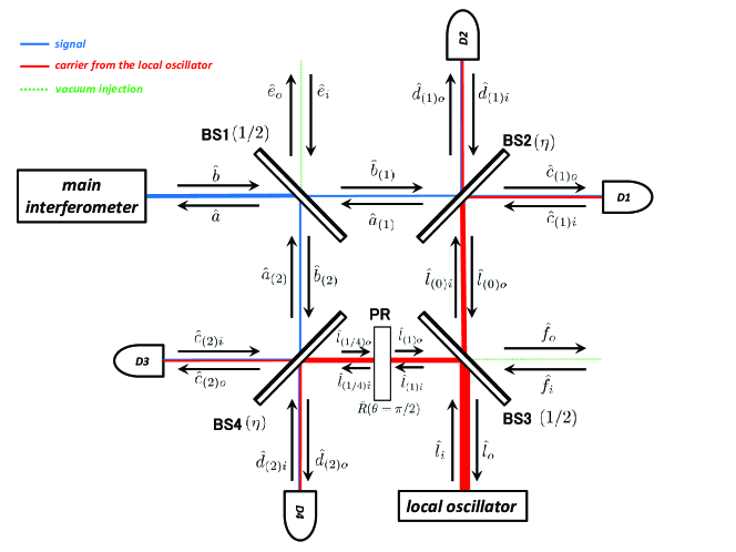
Figure 3: A relaization of the meaurement process of the quadrature $\langle\hat{b}_{\theta}\rangle$. “BS” is the beam splitter and “PR” is the phase rotator. To measure the expectation values (105) and (108) at the same time, we introduce two balanced homodyne detection. To carry out these two balanced homodyne detections, we separate the signal photon field associated with the quadrature $\hat{b}$ from the main interferometer and the photon field associated with the quadrature $\hat{l}_{i}$ from the local oscillator through the beam splitters BS1 and BS3, respectively. One of these two paths is used for the usual balanced homodyne detection through the beam splitter BS2 and the photodetectors D1 and D2. Along the other path, we introduce the phase rotator PR to introduce $\pi/2$-phase difference in the photon field from the local oscillator and detect by the usual balanced homodyne detection through the beam splitter B4 and the photodetector D3 and D2 after this phase addition. We describe the paths of the signal photon field and the field from the local oscillator. The notation of the quadratures for the photon fields are also described in this figure. We consider the case where the transmittance $\eta$ for BS2 and BS4 is not $1/2$ as a simple model of imperfection of the interferometer setup.

IV.2.1 Outline of double balanced homodyne detection

To measure the expectation values (105) and (108) at the same time, we introduce two balanced homodyne detections. To carry out these two balanced homodyne detection, through the beam splitter BS1, we separate the signal photon field associated with the quadrature $\hat{b}$ from the main interferometer. Furthermore, through the beam splitter BS3, we also separate the photon field associated with the quadrature $\hat{l}_{i}$ from the local oscillator. One of the these separated set of the signal field associated with the quadrature $\hat{b}_{(1)}$ and the field associated with the quadrature $\hat{l}_{(0)}$ from the local oscillator are mixed at the beam splitter BS2 and this mixed fields are detected by photodetectors D1 and D2 to carry out the usual balanced homodyne detection. In another set of these separated operator, the field from the local oscillator associated with the quadrature $\hat{l}_{(1)i}$ goes through the phase rotator PR and gain the additional $\pi/2$-phase. We denote the quadrature for this phase-added field by $\hat{l}_{(1/4)i}$. This field and the separated signal field associated with the quadrature $\hat{b}_{(2)}$ are mixed the beam splitter BS4 and then detected by the photodetectors D3 and D4 to carry out the usual balanced homodyne detection.

IV.2.2 Separation of the signal field

From here, we analyze the photon fields according to the interferometer setup depicted in Fig. 3, in detail.

First, at the 50:50 beam splitter 1 (BS1), the output signal $\hat{b}$ from the main interferometer is separated into two parts, which we denote $\hat{b}_{(1)}$ and $\hat{b}_{(2)}$, respectively. In addition to the output quadrature $\hat{b}$, the additional noise source is inserted, which is denoted $\hat{e}_{i}$ in Fig. 3. Then, at BS1, the quadratures $\hat{b}$, $\hat{b}_{(1)}$, $\hat{b}_{(2)}$, and $\hat{e}_{i}$ are related as

$$\hat{b}_{(1)}=\frac{1}{\sqrt{2}}\left(\hat{b}-\hat{e}_{i}\right),\quad\hat{b}_{(2)}=\frac{1}{\sqrt{2}}\left(\hat{b}+\hat{e}_{i}\right)$$ (110)

through the field junction conditions at the BS1. We assume the state associated with the quadrature $\hat{e}_{i}$ is vacuum.

IV.2.3 Separation of the field from the local oscillator

At the 50:50 beam splitter 3 (BS3), the incident electric field from the local oscillator is in the coherent state and its quadrature is denoted by $\hat{l}_{i}$. Furthermore, from the configuration depicted in Fig. 3, another incident field to BS3, which we denote its quadrature by $\hat{f}_{i}$, should be taken into account. On the other hand, the beam splitter BS3 separate the electric field into two paths. The electric field along one of these two paths goes from BS3 to BS2. We denote the quadrature associated with this electric field by $\hat{l}_{(0)i}$. On the other hand, the electric field along another path from BS3 is towards to the beam splitter 4 (BS4). We denote the quadrature associated with this electric field by $\hat{l}_{(1)i}$. By the beam splitter condition, quadratures $\hat{l}_{(0)i}$ and $\hat{l}_{(1)i}$ are determined by the equation

$$\hat{l}_{(0)i}=\frac{1}{\sqrt{2}}\left(\hat{l}_{i}-\hat{f}_{i}\right),\quad\hat{l}_{(1)i}=\frac{1}{\sqrt{2}}\left(\hat{l}_{i}+\hat{f}_{i}\right).$$ (111)

We also assume that the state associated with the quadrature $\hat{f}_{i}$ is also vacuum. The field associated with the quadrature $\hat{l}_{(0)i}$ is used in the balanced homodyne detection through the beam splitter 2 (BS2).

To make $\pi/2$-phase difference in the electric field from the local oscillator as discussed in Sec. IV.1, we introduce the phase rotator (PR) between BS3 and BS4. As shown in Appendix A in Ref. H.J.Kimble-Y.Levin-A.B.Matsko-K.S.Thorne-S.P.Vyatchanin-2001 , the phase rotator operates the rotation operator $\hat{R}(\theta)$ defined by

$$\hat{R}(\theta)=\exp\left\{-i\theta\int_{0}^{+\infty}\frac{d\Omega}{2\pi}\left(\hat{l}_{(1)i+}^{\dagger}\hat{l}_{(1)i+}+\hat{l}_{(1)i-}^{\dagger}\hat{l}_{(1)i-}\right)\right\}.$$ (112)

The phase rotator (PR) in Fig. 3 is defined as a device which operates to the quadrature $\hat{l}_{(1)i}$ and produce the quantum field associated with the quadrature $\hat{l}_{(1/4)i}$ as the output field as

$$\hat{l}_{(1/4)i}=i\hat{l}_{(1)i}.$$ (113)

This quadrature $\hat{l}_{(1/4)i}$ is used the balanced homodyne detection through BS4.

IV.2.4 Balanced homodyne detection through BS2

Now, we consider the balanced homodyne detection through the beam splitter BS2. Here, we assume that the transmittance of the beamsplitter BS2 is $\eta$ as a simple model of the imperfections of the interferometer configurations. The important incident fields to the beam splitter BS2 are $\hat{b}_{(1)}$ and $\hat{l}_{(0)i}$ and the important outgoing fields from BS2 are $\hat{c}_{(1)o}$ and $\hat{d}_{(1)o}$. At the BS2, these fields are related as

$$\hat{c}_{(1)o}=\sqrt{\eta}\hat{b}_{(1)}+\sqrt{1-\eta}\hat{l}_{(0)i},\quad\hat{d}_{(1)o}=\sqrt{\eta}\hat{l}_{(0)i}-\sqrt{1-\eta}\hat{b}_{(1)}.$$ (114)

The quadrature $\hat{b}_{(1)}$ is related to the direct output quadrature $\hat{b}$ through the first equation in Eqs. (110) and the quadrature $\hat{l}_{(0)i}$ is related to the quadrature $\hat{l}_{i}$ of the incident field from the local oscillator through the first equation in Eqs. (111). Then, Eqs. (114) are given by

$$\hat{c}_{(1)o} = \frac{1}{\sqrt{2}}\left(\sqrt{\eta}\hat{b}+\sqrt{1-\eta}\hat{l}_{i}\right)-\frac{1}{\sqrt{2}}\left(\sqrt{\eta}\hat{e}_{i}+\sqrt{1-\eta}\hat{f}_{i}\right),$$ (115)

$$\hat{d}_{(1)o} = \frac{1}{\sqrt{2}}\left(\sqrt{\eta}\hat{l}_{i}-\sqrt{1-\eta}\hat{b}\right)+\frac{1}{\sqrt{2}}\left(\sqrt{1-\eta}\hat{e}_{i}-\sqrt{\eta}\hat{f}_{i}\right).$$ (116)

Here, we note that the second terms in Eqs. (115) and (116) are the contribution of the incident vacuum field due to the interferometer configuration depicted in Fig. 3, respectively.

The photon numbers of the output fields associated with the quadratures $\hat{c}_{(1)o}$ and $\hat{d}_{(1)o}$ are detected through the photodetector D1 and D2 in Fig. 3, respectively. These photon-number operators are defined by

$$\hat{n}_{c_{(1)o}}:=\hat{c}_{(1)o}^{\dagger}\hat{c}_{(1)o},\quad\hat{n}_{d_{(1)o}}:=\hat{d}_{(1)o}^{\dagger}\hat{d}_{(1)o}.$$ (117)

Through Eqs. (115) and (116), these operators are given in terms of the quadratures $\hat{b}$, $\hat{l}_{i}$, $\hat{e}_{i}$ and $\hat{f}_{i}$. The expectation values of the photon-number operators $\hat{n}_{c_{(1)o}}$ and $\hat{n}_{d_{(1)o}}$, which is detected by the photodetector D1 and D2, respectively, are given by

$$\langle\hat{n}_{c_{(1)o}}\rangle = \frac{\eta}{2}\left\langle\hat{n}_{b}\right\rangle+\frac{\sqrt{\eta(1-\eta)}}{2}\left\langle\gamma^{*}\hat{b}+\gamma\hat{b}^{\dagger}\right\rangle+\frac{(1-\eta)}{2}|\gamma|^{2},$$ (118)

$$\langle\hat{n}_{d_{(1)o}}\rangle = \frac{\eta}{2}|\gamma|^{2}-\frac{\sqrt{\eta(1-\eta)}}{2}\left\langle\gamma^{*}\hat{b}+\gamma\hat{b}^{\dagger}\right\rangle+\frac{1-\eta}{2}\langle\hat{n}_{b}\rangle.$$ (119)

In the derivation of Eqs. (119) and (119), we used the field associated with the quadrature $\hat{l}_{i}$ is in the coherent state with the complex amplitude $\gamma$ and the fields associated with the quadratures $\hat{e}_{i}$ and $\hat{f}_{i}$ are in vacua, respectively. As in the case of the conventional balanced homodyne detection in Sec. II.3, we obtain

$$\frac{2}{\sqrt{\eta(1-\eta)}}\left((1-\eta)\langle\hat{n}_{c_{(1)o}}\rangle-\eta\langle\hat{n}_{d_{(1)o}}\rangle-\frac{1-2\eta}{2}|\gamma|^{2}\right)=\left\langle\gamma^{*}\hat{b}+\gamma\hat{b}^{\dagger}\right\rangle$$ (120)

from Eqs. (119) and (119). Thus, the expectation value of the self-adjoint operator $\gamma^{*}\hat{b}+\gamma\hat{b}^{\dagger}$ can be calculated through the photon-number expectation value $\langle\hat{n}_{c_{(1)o}}\rangle$ and $\langle\hat{n}_{d_{(1)o}}\rangle$, if the non-vanishing complex amplitude $\gamma$ of the coherent state from the local oscillator and the transmittance $\eta$ of the beam splitter are given.

The left-hand side of Eq. (120) is regarded as the expectation value of the operator $\hat{s}_{D1D2}$ defined by

$$\hat{s}_{D1D2}:=\frac{2}{\sqrt{\eta(1-\eta)}}\left((1-\eta)\hat{n}_{c_{(1)o}}-\eta\hat{n}_{d_{(1)o}}-\frac{1-2\eta}{2}|\gamma|^{2}\right).$$ (121)

Through Eqs. (115), (116) and (117), in terms of the quadrature $\hat{b}$, $\hat{l}_{i}$, $\hat{e}_{i}$, and $\hat{f}_{i}$, the operator $\hat{s}_{D1D2}$ defined by Eq. (121) is also expressed as

$$\hat{s}_{D1D2} = \hat{b}\hat{l}_{i}^{\dagger}+\hat{b}^{\dagger}\hat{l}_{i}+\frac{1-2\eta}{\sqrt{\eta(1-\eta)}}\left(\hat{l}_{i}^{\dagger}\hat{l}_{i}-|\gamma|^{2}\right)$$ (122)

$$-\hat{b}\hat{f}_{i}^{\dagger}-\hat{b}^{\dagger}\hat{f}_{i}+\hat{e}_{i}\hat{f}_{i}^{\dagger}+\hat{e}_{i}^{\dagger}\hat{f}_{i}-\hat{e}_{i}\hat{l}_{i}^{\dagger}-\hat{e}_{i}^{\dagger}\hat{l}_{i}$$

$$+\frac{1-2\eta}{\sqrt{\eta(1-\eta)}}\left(\hat{f}_{i}^{\dagger}\hat{f}_{i}-\hat{f}_{i}^{\dagger}\hat{l}_{i}-\hat{l}_{i}^{\dagger}\hat{f}_{i}\right).$$

In the right-hand side of Eq. (122), the first line gives the expectation value (120), the second-line is the contributions from the vacuum inputs, and the final line is the vacuum contribution due to the imperfection of the beam splitter BS2.

IV.2.5 Balanced homodyne detection through BS4

Next, we consider the balanced homodyne detection through the beam splitter BS4. Here, we again assume that the transmittance of the beamsplitter BS4 is $\eta$, as a simple model of the imperfections of the interferometer configurations. The important incident fields to the beam splitter BS4 is $\hat{b}_{(2)}$ and $\hat{l}_{(1/4)i}$ and the important outgoing fields from BS4 is $\hat{c}_{(2)o}$ and $\hat{d}_{(2)o}$. At the BS4, these fields are related as

$$\hat{c}_{(2)o}=\sqrt{\eta}\hat{l}_{(1/4)i}-\sqrt{1-\eta}\hat{b}_{(2)},\quad\hat{d}_{(2)o}=\sqrt{\eta}\hat{b}_{(2)}+\sqrt{1-\eta}\hat{l}_{(1/4)i}.$$ (123)

Here, we consider the case where the transmittance of the beam splitter BS4 is also $\eta$, which equal to the transmittance of the beam splitter BS2, as a simple model of imperfections of the interferometer setup.

The quadrature $\hat{b}_{(2)}$ is related to the direct output quadrature $\hat{b}$ through the second equation in Eqs. (110). On the other hand, the quadrature $\hat{l}_{(1/4)i}$ is related to the quadrature $\hat{l}_{i}$ of the incident field from the local oscillator through the second equation of Eqs. (111) and the effect of the phase rotator (113). Then, Eqs. (123) are given by

$$\hat{c}_{(2)o} = \frac{1}{\sqrt{2}}\left(i\sqrt{\eta}\hat{l}_{i}-\sqrt{1-\eta}\hat{b}\right)+\frac{1}{\sqrt{2}}\left(i\sqrt{\eta}\hat{f}_{i}-\sqrt{1-\eta}\hat{e}_{i}\right),$$ (124)

$$\hat{d}_{(2)o} = \frac{1}{\sqrt{2}}\left(\sqrt{\eta}\hat{b}+i\sqrt{1-\eta}\hat{l}_{i}\right)+\frac{1}{\sqrt{2}}\left(\sqrt{\eta}\hat{e}_{i}+i\sqrt{1-\eta}\hat{f}_{i}\right).$$ (125)

Here, we note that the second terms in Eqs. (124) and (125) are the contribution of the incident vacuum field due to the interferometer configuration depicted in Fig. 3, respectively.

The photon numbers of the output fields associated with the quadratures $\hat{c}_{(2)o}$ and $\hat{d}_{(2)o}$ are detected through the photodetector D3 and D4 in Fig. 3, respectively. These photon-number operators are defined by

$$\hat{n}_{c_{(2)o}}:=\hat{c}_{(2)o}^{\dagger}\hat{c}_{(2)o},\quad\hat{n}_{d_{(2)o}}:=\hat{d}_{(2)o}^{\dagger}\hat{d}_{(2)o}.$$ (126)

Through Eqs. (124) and (125), these operators are given in terms of the quadratures $\hat{b}$, $\hat{l}_{i}$, $\hat{e}_{i}$ and $\hat{f}_{i}$. The expectation values of the photon number operators $\hat{n}_{c_{(2)}o}$ and $\hat{n}_{d_{(2)o}}$, which are detected by the photodetector D3 and D4, respectively, are given by

$$\langle\hat{n}_{c_{(2)o}}\rangle = \frac{\eta}{2}|\gamma|^{2}+\frac{i\sqrt{\eta(1-\eta)}}{2}\left\langle\gamma^{*}\hat{b}-\gamma\hat{b}^{\dagger}\right\rangle+\frac{1-\eta}{2}\left\langle\hat{n}_{b}\right\rangle,$$ (127)

$$\langle\hat{n}_{d_{(2)o}}\rangle = \frac{\eta}{2}\left\langle\hat{n}_{b}\right\rangle-\frac{i\sqrt{\eta(1-\eta)}}{2}\left\langle\gamma^{*}\hat{b}-\gamma\hat{b}^{\dagger}\right\rangle+\frac{1-\eta}{2}|\gamma|^{2}.$$ (128)

In the derivation of Eqs. (127) and (128), we used the field associated with the quadrature $\hat{l}_{i}$ is in the coherent state with the complex amplitude $\gamma$ and the fields associated with the quadratures $\hat{e}_{i}$ and $\hat{f}_{i}$ are in vacua. As in the case of the conventional balanced homodyne detection in Sec. II.3, we obtain

$$-\frac{2i}{\sqrt{\eta(1-\eta)}}\left(\eta\langle\hat{n}_{c_{(2)o}}\rangle-(1-\eta)\langle\hat{n}_{d_{(2)o}}\rangle+\frac{1-2\eta}{2}|\gamma|^{2}\right)=\left\langle\gamma^{*}\hat{b}-\gamma\hat{b}^{\dagger}\right\rangle.$$ (129)

from Eqs. (127) and (128). Thus, the expectation value of the anti-self-adjoint operator $\gamma^{*}\hat{b}-\gamma\hat{b}^{\dagger}$ can be calculated through the photon number expectation value $\langle\hat{n}_{c_{(2)o}}\rangle$ and $\langle\hat{n}_{d_{(2)o}}\rangle$, if the complex amplitude $\gamma$ of the coherent state from the local oscillator and the transmittance $\eta$ of the beam splitters B2 and B4 are given.

The left-hand side of Eq. (129) is regarded as the expectation value of the operator $\hat{s}_{D3D4}(\omega)$ defined by

$$\hat{s}_{D3D4}:=\frac{2i}{\sqrt{\eta(1-\eta)}}\left((1-\eta)\hat{n}_{d_{(2)o}}-\eta\hat{n}_{c_{(2)o}}-\frac{1-2\eta}{2}|\gamma|^{2}\right).$$ (130)

Through Eqs. (124), (125), and (126), in terms of the quadrature $\hat{b}$, $\hat{l}_{i}$, $\hat{e}_{i}$, and $\hat{f}_{i}$, the operator $\hat{s}_{D3D4}$ defined by Eq. (130) is also expressed as

$$\hat{s}_{D3D4} = \hat{l}_{i}^{\dagger}\hat{b}-\hat{b}^{\dagger}\hat{l}_{i}+\frac{i(1-2\eta)}{\sqrt{\eta(1-\eta)}}\left(\hat{l}_{i}^{\dagger}\hat{l}_{i}-|\gamma|^{2}\right)$$ (131)

$$-\hat{b}^{\dagger}\hat{f}_{i}+\hat{b}\hat{f}_{i}^{\dagger}+\hat{l}_{i}^{\dagger}\hat{e}_{i}+\hat{f}_{i}^{\dagger}\hat{e}_{i}-\hat{e}_{i}^{\dagger}\hat{l}_{i}-\hat{e}_{i}^{\dagger}\hat{f}_{i}$$

$$+\frac{i(1-2\eta)}{\sqrt{\eta(1-\eta)}}\left(\hat{f}_{i}^{\dagger}\hat{l}_{i}+\hat{l}_{i}^{\dagger}\hat{f}_{i}+\hat{f}_{i}^{\dagger}\hat{f}_{i}\right).$$

In the right-hand side of Eq. (131), the first line gives the expectation value (129), the second-line is the contributions from the vacuum inputs, and the final line is the vacuum contribution due to the unbalance of the beam splitter BS4.

We note that the overall factor in the left-hand side of Eq. (129) and the right-hand side of the definition (130) are purely imaginary. These factors breaks the self-adjointness of our results.

IV.3 Input vacuum to the main interferometer

The output operators (122) and (131) to measure the operator $\hat{b}$ or $\hat{b}^{\dagger}$ are described by the quadratures $\hat{b}$, $\hat{l}_{i}$, $\hat{e}_{i}$, and $\hat{f}_{i}$. As depicted in Fig. 3, $\hat{e}_{i}$, $\hat{f}_{i}$, and $\hat{l}_{i}$ are quadratures of the independent fields. Then, we should regard that these operators commute with each other:

$$\left[\hat{e}_{i},\hat{f}_{i}\right]=\left[\hat{e}_{i},\hat{f}_{i}^{\dagger}\right]=\left[\hat{f}_{i},\hat{l}_{i}\right]=\left[\hat{f}_{i},\hat{l}_{i}^{\dagger}\right]=\left[\hat{l}_{i},\hat{e}_{i}\right]=\left[\hat{l}_{i},\hat{e}_{i}^{\dagger}\right]=0.$$ (132)

The main purpose of this subsection is to check whether or not we may regard the output quadrature $\hat{b}$ is also independent of $\hat{e}_{i}$, $\hat{f}_{i}$, and $\hat{l}_{i}$.

To check this independence, we have to remind that the operator $\hat{b}$ is the output quadrature from the main interferometer and we have the input quadrature $\hat{a}$ to the main interferometer. In general, the output quadrature $\hat{b}$ may depend on this input quadrature $\hat{a}$. In many situation, we regard that the field associated with the quadrature $\hat{a}$ is in vacuum. Here, we check this vacuum state for the quadrature $\hat{a}$ is an independent vacuum from the states of the photon fields associated with the quadratures $\hat{e}_{i}$, $\hat{f}_{i}$, and $\hat{l}_{i}$ through the interferometer configuration depicted in Fig. 3.

At the BS1, the quadrature $\hat{a}$ is given by

$$\hat{a}=\frac{1}{\sqrt{2}}\left(\hat{a}_{(1)}+\hat{a}_{(2)}\right),$$ (133)

and, at the BS2, the quadrature $\hat{a}_{(1)}$ is given by

$$\hat{a}_{(1)}=\sqrt{\eta}\hat{c}_{(1)i}-\sqrt{1-\eta}\hat{d}_{(1)i}.$$ (134)

The quadratures $\hat{c}_{(1)i}$ and $\hat{d}_{(1)i}$ are the quadratures of the incident fields from detectors D1 and D2 to the BS2, respectively. On the other hand, through the junction at the BS4, the quadrature $\hat{a}_{(2)}$ is given by

$$\hat{a}_{(2)}=\sqrt{\eta}\hat{d}_{(2)i}-\sqrt{1-\eta}\hat{c}_{(2)i}.$$ (135)

The quadratures $\hat{c}_{(2)i}$ and $\hat{d}_{(2)i}$ are the quadratures of the incident fields from detectors D3 and D4 to the BS4, respectively.

Substituting Eqs. (134) and (135) into Eq. (133), we obtain

$$\hat{a}=\sqrt{\frac{\eta}{2}}\left(\hat{c}_{(1)i}+\hat{d}_{(2)i}\right)-\sqrt{\frac{1-\eta}{2}}\left(\hat{d}_{(1)i}+\hat{c}_{(2)i}\right).$$ (136)

We assume that the states associated with the quadratures $\hat{c}_{(1)i}$, $\hat{c}_{(2)i}$, $\hat{d}_{(1)i}$, and $\hat{d}_{(2)i}$ from the detectors D1, D3, D2, and D4 are vacua. Due to this situation, the state associated with the input quadrature $\hat{a}$ is also regarded as a vacuum. Furthermore, Eq. (136) indicates that the quadrature $\hat{a}$ is independent of the quadratures $\hat{e}_{i}$, $\hat{f}_{i}$, and $\hat{l}_{i}$. Therefore, we may regard that

$$\left[\hat{a},\hat{e}_{i}\right]=\left[\hat{a},\hat{e}_{i}^{\dagger}\right]=\left[\hat{a},\hat{f}_{i}\right]=\left[\hat{a},\hat{f}_{i}^{\dagger}\right]=\left[\hat{a},\hat{l}_{i}\right]=\left[\hat{a},\hat{l}_{i}^{\dagger}\right]=0,$$ (137)

and then, we may regard that

$$\left[\hat{b},\hat{e}_{i}\right]=\left[\hat{b},\hat{e}_{i}^{\dagger}\right]=\left[\hat{b},\hat{f}_{i}\right]=\left[\hat{b},\hat{f}_{i}^{\dagger}\right]=\left[\hat{b},\hat{l}_{i}\right]=\left[\hat{b},\hat{l}_{i}^{\dagger}\right]=0,$$ (138)

even if the output quadrature $\hat{b}$ depends on the input quadrature $\hat{a}$.

We use the commutation relations (132) and (138) when we evaluate the fluctuations in the measurements discussed in Sec. IV.4 and Sec. IV.5.

IV.4 Measurements of an annihilation operator $\hat{b}$ and a creation operator $\hat{b}^{\dagger}$

In Sec. IV.2, the expectation value of the operators $\hat{s}_{D1D2}$ and $\hat{s}_{D3D4}$ can be calculated through the photon-number expectation values at the photodetectors D1, D2, D3, and D4. In this subsection, we note that we can calculate the expectation values of the annihilation and creation operators of photon field from the expectation values of these operators. The simplified version of the ingredients of this subsection is already explained in Ref. K.Nakamura-M.-K.Fujimoto-2017b .

Note that the field associated with the quadrature $\hat{l}_{i}$ is in the coherent state with the complex amplitude $\gamma$ and the fields associated with the quadratures $\hat{f}_{i}$ and $\hat{e}_{i}$ are in their vacuum states in the derivation of the form of the operators $\hat{s}_{D1D2}$ and $\hat{s}_{D3D4}$. The guiding principle of the construction of the operators $\hat{s}_{D1D2}$ and $\hat{s}_{D3D4}$ are just their expectation values which are given by (120) and (129). From these expectation values, the expectation values of $\langle\hat{b}\rangle$ and $\langle\hat{b}^{\dagger}\rangle$ are given by

$$\frac{1}{2\gamma^{*}}\left(\left\langle\hat{s}_{D1D2}\right\rangle+\left\langle\hat{s}_{D3D4}\right\rangle\right)=\left\langle\hat{b}\right\rangle,$$ (139)

$$\frac{1}{2\gamma}\left(\left\langle\hat{s}_{D1D2}\right\rangle-\left\langle\hat{s}_{D3D4}\right\rangle\right)=\left\langle\hat{b}^{\dagger}\right\rangle.$$ (140)

These are assertions which is pointed out in Ref. K.Nakamura-M.-K.Fujimoto-2017b and are trivial result from the construction of the operators $\hat{s}_{D1D2}$ and $\hat{s}_{D3D4}$. We have to emphasize that the expectation values of the operators $\hat{s}_{D1D2}$ and $\hat{s}_{D3D4}$ are calculable through the expectation values of photon number operators which are measured at the photodetector D1, D2, D3, and D4, the complex amplitude $\gamma$ for the coherent state from the local oscillator, and the transmittance $\eta$ of the beam splitters B2 and B4. A similar assertion was also reported in Ref. E.Shchukin-Th.Richter-W.Vogel-2005 in the context of the nonclassicality criteria of quantum system.

Here, we also note that the direct calculation from Eqs. (122) and (131) yields

$$\hat{t}_{b+} := \frac{1}{2\gamma^{*}}\left(\hat{s}_{D1D2}+\hat{s}_{D3D4}\right)$$ (141)

$$= \hat{b}\frac{\hat{l}_{i}^{\dagger}}{\gamma^{*}}+\frac{(1+i)(1-2\eta)}{2\sqrt{\eta(1-\eta)}}\gamma\left(\frac{\hat{l}_{i}^{\dagger}\hat{l}_{i}}{|\gamma|^{2}}-1\right)$$

$$+\frac{1}{\gamma^{*}}\left(-\hat{b}^{\dagger}\hat{f}_{i}+\hat{e}_{i}\hat{f}_{i}^{\dagger}-\hat{e}_{i}^{\dagger}\hat{l}_{i}\right)$$

$$+\frac{(1+i)(1-2\eta)}{2\sqrt{\eta(1-\eta)}\gamma^{*}}\left(+i\hat{f}_{i}^{\dagger}\hat{f}_{i}-\hat{f}_{i}^{\dagger}\hat{l}_{i}-\hat{l}_{i}^{\dagger}\hat{f}_{i}\right).$$

and

$$\hat{t}_{b-} := \frac{1}{2\gamma}\left(\hat{s}_{D1D2}-\hat{s}_{D3D4}\right)$$ (142)

$$= \hat{b}^{\dagger}\frac{\hat{l}_{i}}{\gamma}+\frac{(1-i)(1-2\eta)}{2\sqrt{\eta(1-\eta)}}\gamma^{*}\left(\frac{\hat{l}_{i}^{\dagger}\hat{l}_{i}}{|\gamma|^{2}}-1\right)$$

$$+\frac{1}{\gamma}\left(-\hat{b}\hat{f}_{i}^{\dagger}+\hat{e}_{i}^{\dagger}\hat{f}_{i}-\hat{e}_{i}\hat{l}_{i}^{\dagger}\right)$$

$$+\frac{(1-i)(1-2\eta)}{2\sqrt{\eta(1-\eta)}\gamma}\left(-i\hat{f}_{i}^{\dagger}\hat{f}_{i}-\hat{l}_{i}^{\dagger}\hat{f}_{i}-\hat{f}_{i}^{\dagger}\hat{l}_{i}\right).$$

We also note that

$$\hat{t}_{b+}^{\dagger}=\hat{t}_{b-}$$ (143)

from the explicit expression (141) and (142).

Through the explicit expression of the operators (141) and (142), we evaluate the fluctuations in the measurement of the expectation values (139) and (140). Since the operators $\hat{t}_{b\pm}$ are not self-adjoint as in Eq. (143), there is no guiding principle to evaluate their fluctuations, in general. In this paper, we evaluate the fluctuations through the expectation value

$$\left\langle\frac{1}{2}\left(\hat{t}_{b\pm}(\omega)\hat{t}_{b\pm}^{\dagger}(\omega^{\prime})+\hat{t}_{b\pm}^{\dagger}(\omega^{\prime})\hat{t}_{b\pm}(\omega)\right)\right\rangle.$$ (144)

The evaluation through Eq. (144) is commonly used to evaluate spectral densities of gravitational-wave detectors H.J.Kimble-Y.Levin-A.B.Matsko-K.S.Thorne-S.P.Vyatchanin-2001 ; H.Miao-PhDthesis-2010 . Furthermore, the operator $\hat{t}_{b\pm}$ has the property (143), the expectation value Eq. (144) is evaluated as

$$\left\langle\frac{1}{2}\left(\hat{t}_{b\pm}(\omega)\hat{t}_{b\pm}^{\dagger}(\omega^{\prime})+\hat{t}_{b\pm}^{\dagger}(\omega^{\prime})\hat{t}_{b\pm}(\omega)\right)\right\rangle=\frac{1}{2}\left(\langle\hat{t}_{b\pm}(\omega)|\hat{t}_{b\mp}(\omega^{\prime})\rangle+\langle\hat{t}_{b\mp}(\omega^{\prime})|\hat{t}_{b\pm}(\omega)\rangle\right),$$ (145)

where we defined

$$|\hat{t}_{b\pm}(\omega)\rangle:=\hat{t}_{b\pm}(\omega)|\Psi\rangle.$$ (146)

Furthermore, we note that

$$\hat{t}_{b+}(\omega^{\prime})\hat{t}_{b+}^{\dagger}(\omega)+\hat{t}_{b+}^{\dagger}(\omega)\hat{t}_{b+}(\omega^{\prime}) = \hat{t}_{b+}(\omega^{\prime})\hat{t}_{b-}(\omega)+\hat{t}_{b-}(\omega)\hat{t}_{b+}(\omega^{\prime})$$ (147)

$$= \hat{t}_{b-}^{\dagger}(\omega^{\prime})\hat{t}_{b-}(\omega)+\hat{t}_{b-}(\omega)\hat{t}_{b-}^{\dagger}(\omega^{\prime}).$$

This implies that the fluctuations in the measurement of the operator $\hat{t}_{b-}$ through Eq. (144) is given by the fluctuations in the measurement of the operator $\hat{t}_{b-}$ through Eq. (144) and the replacement $\omega\leftrightarrow\omega^{\prime}$. For this reason, we only show the results of the fluctuations in the measurement of the expectation value of the operator $\hat{t}_{b+}$:

$$\frac{1}{2}\left\langle\hat{t}_{b+}\hat{t}_{b+}^{{}^{\prime}\dagger}+\hat{t}_{b+}^{{}^{\prime}\dagger}\hat{t}_{b+}\right\rangle = \left\langle\frac{1}{2}\left(\hat{b}^{{}^{\prime}\dagger}\hat{b}+\hat{b}\hat{b}^{{}^{\prime}\dagger}\right)\right\rangle$$ (148)

$$+\left(\frac{\langle\hat{n}_{b}\rangle}{|\gamma|^{2}}+\frac{1}{2}\right)2\pi\delta(\omega-\omega^{\prime})$$

$$+\frac{1-2\eta}{4\sqrt{\eta(1-\eta)}|\gamma|^{2}}\left\langle\gamma^{*}(\gamma^{*}+1)\hat{b}+\gamma(\gamma+1)\hat{b}^{\dagger}\right\rangle 2\pi\delta(\omega-\omega^{\prime})$$

$$+i\frac{1-2\eta}{4\sqrt{\eta(1-\eta)}|\gamma|^{2}}\left\langle\gamma^{*}(\gamma^{*}-1)\hat{b}-\gamma(\gamma-1)\hat{b}^{\dagger}\right\rangle 2\pi\delta(\omega-\omega^{\prime})$$

$$+\frac{(1-2\eta)^{2}}{2\eta(1-\eta)}\left(1+|\gamma|^{2}\right)2\pi\delta(\omega-\omega^{\prime}).$$

Here, we note that the second line of the light-hand side of Eq. (148) comes from the shot noise contribution of the additional input vacua in the interferometer and the remaining lines of the right-hand side is due to the imperfection of the beam splitters BS2 and BS4 from 50:50.

Since we are concentrating on the case where the operators $\hat{t}_{b\pm}$, $\hat{b}$, and $\hat{b}^{\dagger}$ have the nontrivial expectation values $\langle\hat{t}_{b+}\rangle=\langle\hat{b}\rangle$ and $\langle\hat{t}_{b-}\rangle=\langle\hat{b}^{\dagger}\rangle$, Eq. (148) includes not only the information of the fluctuations but also the information of the correlation of these expectation values. Therefore, to consider the fluctuations in the measurements of $\hat{t}_{b\pm}$, we have to eliminate the information of the correlation of the expectation values $\langle\hat{t}_{b+}\rangle=\langle\hat{b}\rangle$ and $\langle\hat{t}_{b-}\rangle=\langle\hat{b}^{\dagger}\rangle$ from Eq. (148). Actually, if we define the noise operator $\hat{t}_{b\pm}^{(n)}$ and $\hat{b}^{(n)}$ so that

$$\hat{t}_{b+} =: \langle\hat{b}\rangle+\hat{t}_{b+}^{(n)},\quad\langle\hat{t}_{b+}^{(n)}\rangle=0,$$ (149)

$$\hat{t}_{b-} =: \langle\hat{b}^{\dagger}\rangle+\hat{t}_{b-}^{(n)},\quad\langle\hat{t}_{b-}^{(n)}\rangle=0,$$ (150)

$$\hat{b} =: \langle\hat{b}\rangle+\hat{b}^{(n)},\quad\langle\hat{b}^{(n)}\rangle=0,$$ (151)

the left-hand side of Eq. (148) and the first term in the right-hand side of Eq. (148) yield

$$\frac{1}{2}\left\langle\hat{t}_{b+}\hat{t}_{b+}^{{}^{\prime}\dagger}+\hat{t}_{b+}^{{}^{\prime}\dagger}\hat{t}_{b+}\right\rangle = \frac{1}{2}\left\langle\hat{t}_{b+}^{(n)}\hat{t}_{b+}^{(n)^{\prime}\dagger}+\hat{t}_{b+}^{(n)^{\prime}\dagger}\hat{t}_{b+}^{(n)}\right\rangle+\langle\hat{b}^{\prime}\rangle^{*}\langle\hat{b}\rangle,$$ (152)

$$\frac{1}{2}\left\langle\hat{b}\hat{b}^{{}^{\prime}\dagger}+\hat{b}^{{}^{\prime}\dagger}\hat{b}\right\rangle = \frac{1}{2}\left\langle\hat{b}^{(n)}\hat{b}^{(n)^{\prime}\dagger}+\hat{b}^{(n)^{\prime}\dagger}\hat{b}^{(n)}\right\rangle+\langle\hat{b}^{\prime}\rangle^{*}\langle\hat{b}\rangle.$$ (153)

In the right-hand side of Eqs. (152) and (153), the first terms corresponds to the noise correlation in the measurements of operators $\hat{b}$ and $\hat{b}^{\dagger}$.

For the quantum operator $\hat{Q}$ with its expectation value $\langle\hat{Q}\rangle=0$, we introduce the noise spectral density as in Refs. H.J.Kimble-Y.Levin-A.B.Matsko-K.S.Thorne-S.P.Vyatchanin-2001 ; H.Miao-PhDthesis-2010 by

$$\frac{1}{2}S_{\hat{Q}}(\omega)2\pi\delta(\omega-\omega^{\prime}):=\frac{1}{2}\left(\hat{Q}(\omega)\hat{Q}^{\dagger}(\omega^{\prime})+\hat{Q}^{\dagger}(\omega^{\prime})\hat{Q}(\omega)\right).$$ (154)

Then, Eq. (148) yields the relation between the noise spectral densities as

$$S_{\hat{t}_{b+}^{(n)}}(\omega) = S_{\hat{b}^{(n)}}(\omega)+\frac{2\langle\hat{n}_{b}\rangle}{|\gamma|^{2}}+1$$ (155)

$$+\frac{1-2\eta}{2\sqrt{\eta(1-\eta)}|\gamma|^{2}}\left\langle\gamma^{*}(\gamma^{*}+1)\hat{b}+\gamma(\gamma+1)\hat{b}^{\dagger}\right\rangle$$

$$+i\frac{1-2\eta}{2\sqrt{\eta(1-\eta)}|\gamma|^{2}}\left\langle\gamma^{*}(\gamma^{*}-1)\hat{b}-\gamma(\gamma-1)\hat{b}^{\dagger}\right\rangle$$

$$+\frac{(1-2\eta)^{2}}{\eta(1-\eta)}\left(1+|\gamma|^{2}\right).$$

Equation (155) indicates that the imperfection $\eta$ of the beam splitter gives additional noise. On the other hand, in the case where the beam splitters BS2 and BS4 is 50:50, i.e., $\eta=1/2$, equation (155) gives

$$S_{\hat{t}_{b+}^{(n)}}(\omega) = S_{\hat{b}^{(n)}}(\omega)+\frac{2}{|\gamma|^{2}}\langle\hat{n}_{b}\rangle+1.$$ (156)

This is the result which was shown in Ref. K.Nakamura-M.-K.Fujimoto-2017b and the similar result is previously reported E.Shchukin-Th.Richter-W.Vogel-2005 in the context of the characterization of the non-classicality for a quantum system. Equation (156) indicates that in addition to the noise spectral density $S_{\hat{b}^{(n)}}(\omega)$, we have the additional fluctuations which described by $2\langle\hat{n}_{b}\rangle/|\gamma^{2}|+1$ in the double balanced homodyne detection to measure $\hat{b}$ through the measurement of $\hat{t}_{b+}$. We note that the term $2\langle\hat{n}_{b}\rangle/|\gamma^{2}|$ will be negligible if the absolute value of the complex amplitude $\gamma$ is much larger than the expectation value of the output photon number $\langle\hat{n}_{b}\rangle$, i.e., $\langle\hat{n}_{b}\rangle\ll|\gamma^{2}|$. On the other hand, the term $1$ in $2\langle\hat{n}_{b}\rangle/|\gamma^{2}|+1$, which comes from the shot noise from the additional input vacuum fields in the interferometer for the double balanced homodyne detection, is not controllable. Furthermore, the comparison of Eqs. (155) and (156) indicates that the the behavior of the noise spectrum density $S_{\hat{t}_{b+}^{(n)}}(\omega)$ is sensitive to the transmittance $\eta$. In particular, the last term in Eq. (155) may become dominant when $|\gamma|\gg 1$.

IV.5 Double balanced homodyne detection in two-photon description

Here, we consider the two-photon description and show that we can calculate the expectation value of the operator $\hat{b}_{\theta}$ through the interferometer setup depicted in Fig. 3.

As discussed in Sec. III, we consider the sideband with the frequencies $\omega_{0}\pm\Omega$. The output through the balanced homodyne detection using D1 and D2 has the information of the operators $\hat{s}_{D1D2}(\omega_{0}\pm\Omega)=\hat{s}_{D1D2\pm}$ defined by

$$\hat{s}_{D1D2\pm} = \hat{b}_{\pm}\hat{l}_{i\pm}^{\dagger}+\hat{b}_{\pm}^{\dagger}\hat{l}_{i\pm}+\frac{1-2\eta}{\sqrt{\eta(1-\eta)}}\left(\hat{l}_{i\pm}^{\dagger}\hat{l}_{i\pm}-|\gamma_{\pm}|^{2}\right)$$ (157)

$$-\hat{b}_{\pm}\hat{f}_{i\pm}^{\dagger}-\hat{b}_{\pm}^{\dagger}\hat{f}_{i\pm}+\hat{e}_{i\pm}\hat{f}_{i\pm}^{\dagger}+\hat{e}_{i\pm}^{\dagger}\hat{f}_{i\pm}-\hat{e}_{i\pm}\hat{l}_{i\pm}^{\dagger}-\hat{e}_{i\pm}^{\dagger}\hat{l}_{i\pm}$$

$$+\frac{1-2\eta}{\sqrt{\eta(1-\eta)}}\left(\hat{f}_{i\pm}^{\dagger}\hat{f}_{i\pm}-\hat{f}_{i\pm}^{\dagger}\hat{l}_{i\pm}-\hat{l}_{i\pm}^{\dagger}\hat{f}_{i\pm}\right)$$

from Eq. (122). Following the discussion in Sec. IV.1.2, we introduce the operators $\hat{t}_{D1D2+}$ defined by

$$\hat{t}_{D1D2+}:=\frac{1}{\sqrt{2}}\left(\frac{\hat{s}_{D1D2+}}{|\gamma_{+}|}+\frac{\hat{s}_{D1D2-}}{|\gamma_{-}|}\right),$$ (158)

where the electric field assoicated with the quadratures $\hat{l}_{i\pm}$ are in the coherent state with the complex amplitude $\gamma_{\pm}$ and the phase $\theta_{\pm}$ of $\gamma_{\pm}$ is chosen so that $\theta_{\pm}$ $=$ $\theta$ and $|\gamma_{+}|$ $=$ $|\gamma_{-}|$ $=:$ $|\gamma|$. This choice of the phase is essential for the measurement of the expectation value $\langle\hat{b}_{\theta}\rangle$. Under this situation, we evaluate the operator $\hat{t}_{D1D2+}$ defined by Eqs. (158). Substituting Eqs. (157) into Eq. (158) and using the definitions (34) of the operators $\hat{b}_{1}$ and $\hat{b}_{2}$, we obtain

$$\hat{t}_{D1D2+} = \frac{1}{2|\gamma|}\left(\hat{l}_{i-}+\hat{l}_{i+}^{\dagger}\right)\hat{b}_{1}+\frac{1}{2i|\gamma|}\left(\hat{l}_{i-}-\hat{l}_{i+}^{\dagger}\right)\hat{b}_{2}$$ (159)

$$+\frac{1}{2|\gamma|}\left(\hat{l}_{i+}+\hat{l}_{i-}^{\dagger}\right)\hat{b}_{1}^{\dagger}+\frac{1}{2i|\gamma|}\left(\hat{l}_{i+}-\hat{l}_{i-}^{\dagger}\right)\hat{b}_{2}^{\dagger}$$

$$+\frac{1-2\eta}{\sqrt{2\eta(1-\eta)}|\gamma|}\left(\hat{l}_{i+}^{\dagger}\hat{l}_{i+}+\hat{l}_{i-}^{\dagger}\hat{l}_{i-}-2|\gamma|^{2}\right)$$

$$+\frac{1}{\sqrt{2}|\gamma|}\left(-\hat{b}_{+}\hat{f}_{i+}^{\dagger}-\hat{b}_{+}^{\dagger}\hat{f}_{i+}+\hat{e}_{i+}\hat{f}_{i+}^{\dagger}+\hat{e}_{i+}^{\dagger}\hat{f}_{i+}-\hat{e}_{i+}\hat{l}_{i+}^{\dagger}-\hat{e}_{i+}^{\dagger}\hat{l}_{i+}\right)$$

$$+\frac{1}{\sqrt{2}|\gamma|}\left(-\hat{b}_{-}\hat{f}_{i-}^{\dagger}-\hat{b}_{-}^{\dagger}\hat{f}_{i-}+\hat{e}_{i-}\hat{f}_{i-}^{\dagger}+\hat{e}_{i-}^{\dagger}\hat{f}_{i-}-\hat{e}_{i-}\hat{l}_{i-}^{\dagger}-\hat{e}_{i-}^{\dagger}\hat{l}_{i-}\right)$$

$$+\frac{1-2\eta}{\sqrt{2\eta(1-\eta)}}\frac{1}{|\gamma|}\left(\hat{f}_{i+}^{\dagger}\hat{f}_{i+}-\hat{f}_{i+}^{\dagger}\hat{l}_{i+}-\hat{l}_{i+}^{\dagger}\hat{f}_{i+}\right.$$

$$\quad\quad\quad\quad\quad\quad\quad\quad\quad\left.+\hat{f}_{i-}^{\dagger}\hat{f}_{i-}-\hat{f}_{i-}^{\dagger}\hat{l}_{i-}-\hat{l}_{i-}^{\dagger}\hat{f}_{i-}\right).$$

The expectation values of the operator $\hat{t}_{D1D2+}$ is derived from the expectation values of the operator $\hat{s}_{D1D2\pm}$, which are given by the definition (121) and Eq. (120). From these expectation values, we can check that the expectation value of the operator (159) is given by

$$\left\langle\hat{t}_{D1D2+}\right\rangle=\left\langle\cos\theta\hat{b}_{1}+\sin\theta\hat{b}_{2}+\cos\theta\hat{b}_{1}^{\dagger}+\sin\theta\hat{b}_{2}^{\dagger}\right\rangle$$ (160)

On the other hand, the output through the balanced homodyne detection using D3 and D4 has the information of the operators $\hat{s}_{D3D4}(\omega_{0}\pm\Omega)=\hat{s}_{D3D4\pm}$ as

$$\hat{s}_{D3D4\pm} = \hat{l}_{i\pm}^{\dagger}\hat{b}_{\pm}-\hat{b}_{\pm}^{\dagger}\hat{l}_{i\pm}+\frac{i(1-2\eta)}{\sqrt{\eta(1-\eta)}}\left(\hat{l}_{i\pm}^{\dagger}\hat{l}_{i\pm}-|\gamma_{\pm}|^{2}\right)$$ (161)

$$-\hat{b}_{\pm}^{\dagger}\hat{f}_{i\pm}+\hat{b}_{\pm}\hat{f}_{i\pm}^{\dagger}+\hat{l}_{i\pm}^{\dagger}\hat{e}_{i\pm}+\hat{f}_{i\pm}^{\dagger}\hat{e}_{i\pm}-\hat{e}_{i\pm}^{\dagger}\hat{l}_{i\pm}-\hat{e}_{i\pm}^{\dagger}\hat{f}_{i\pm}$$

$$+\frac{i(1-2\eta)}{\sqrt{\eta(1-\eta)}}\left(\hat{f}_{i\pm}^{\dagger}\hat{l}_{i\pm}+\hat{l}_{i\pm}^{\dagger}\hat{f}_{i\pm}+\hat{f}_{i\pm}^{\dagger}\hat{f}_{i\pm}\right).$$

from Eq. (131). Following the discussion in Sec. IV.1.2, we introduce the operator $\hat{t}_{D3D4-}$ defined by

$$\hat{t}_{D3D4-}:=\frac{1}{\sqrt{2}}\left(\frac{\hat{s}_{D3D4+}}{|\gamma_{+}|}-\frac{\hat{s}_{D3D4-}}{|\gamma_{-}|}\right)=\frac{1}{\sqrt{2}|\gamma|}\left(\hat{s}_{D3D4+}-\hat{s}_{D3D4-}\right).$$ (162)

Here, we used our situation where $\theta_{\pm}=\theta$ and $|\gamma_{\pm}|=|\gamma|$. Substituting Eqs. (161) into Eq. (162) and using the definitions (34) of the operators $\hat{b}_{1}$ and $\hat{b}_{2}$, we obtain

$$\hat{t}_{D3D4-} = \frac{1}{2|\gamma|}\left(\hat{l}_{i-}+\hat{l}_{i+}^{\dagger}\right)\hat{b}_{1}+\frac{1}{2i|\gamma|}\left(\hat{l}_{i-}-\hat{l}_{i+}^{\dagger}\right)\hat{b}_{2}$$ (163)

$$-\frac{1}{2|\gamma|}\left(\hat{l}_{i+}+\hat{l}_{i-}^{\dagger}\right)\hat{b}_{1}^{\dagger}-\frac{1}{2i|\gamma|}\left(\hat{l}_{i+}-\hat{l}_{i-}^{\dagger}\right)\hat{b}_{2}^{\dagger}$$

$$+\frac{i(1-2\eta)}{|\gamma|\sqrt{2\eta(1-\eta)}}\left(+\hat{l}_{i+}^{\dagger}\hat{l}_{i+}-\hat{l}_{i-}^{\dagger}\hat{l}_{i-}\right)$$

$$+\frac{1}{\sqrt{2}|\gamma|}\left(-\hat{b}_{+}^{\dagger}\hat{f}_{i+}+\hat{b}_{+}\hat{f}_{i+}^{\dagger}+\hat{l}_{i+}^{\dagger}\hat{e}_{i+}+\hat{f}_{i+}^{\dagger}\hat{e}_{i+}-\hat{e}_{i+}^{\dagger}\hat{l}_{i+}-\hat{e}_{i+}^{\dagger}\hat{f}_{i+}\right)$$

$$+\frac{1}{\sqrt{2}|\gamma|}\left(+\hat{b}_{-}^{\dagger}\hat{f}_{i-}-\hat{b}_{-}\hat{f}_{i-}^{\dagger}-\hat{l}_{i-}^{\dagger}\hat{e}_{i-}-\hat{f}_{i-}^{\dagger}\hat{e}_{i-}+\hat{e}_{i-}^{\dagger}\hat{l}_{i-}+\hat{e}_{i-}^{\dagger}\hat{f}_{i-}\right)$$

$$+\frac{i(1-2\eta)}{|\gamma|\sqrt{2\eta(1-\eta)}}\left(+\hat{f}_{i+}^{\dagger}\hat{l}_{i+}+\hat{l}_{i+}^{\dagger}\hat{f}_{i+}+\hat{f}_{i+}^{\dagger}\hat{f}_{i+}\right.$$

$$\quad\quad\quad\quad\quad\quad\quad\quad\quad\left.-\hat{f}_{i-}^{\dagger}\hat{l}_{i-}-\hat{l}_{i-}^{\dagger}\hat{f}_{i-}-\hat{f}_{i-}^{\dagger}\hat{f}_{i-}\right).$$

As in the case of the operator $\hat{t}_{D1D2+}$, the expectation values of the operators $\hat{s}_{D3D4\pm}$ are given by the definition (130) and Eq. (129). From these expectation values, the expectation values of the operator $\hat{t}_{D3D4-}$ defined by (163) is given by

$$\left\langle\hat{t}_{D3D4-}\right\rangle=\left\langle\cos\theta\hat{b}_{1}+\sin\theta\hat{b}_{2}-\cos\theta\hat{b}_{1}^{\dagger}-\sin\theta\hat{b}_{2}^{\dagger}\right\rangle.$$ (164)

From the expectation values (160) and (164), we obtain the expected result

$$\left\langle\frac{1}{2}\left(\hat{t}_{D1D2+}+\hat{t}_{D3D4-}\right)\right\rangle=\left\langle\cos\theta\hat{b}_{1}+\sin\theta\hat{b}_{2}\right\rangle$$ (165)

Thus, we have derived that the operator whose expectation value yields $\langle\cos\theta\hat{b}_{1}+\sin\theta\hat{b}_{2}\rangle$ is given by

$$\hat{t}_{\theta} := \frac{1}{2}\left(\hat{t}_{D1D2+}+\hat{t}_{D3D4-}\right)$$ (166)

$$= \frac{1}{2\sqrt{2}|\gamma|}\left(\hat{s}_{D1D2+}+\hat{s}_{D1D2-}+\hat{s}_{D3D4+}-\hat{s}_{D3D4-}\right)$$

$$= \frac{1}{2|\gamma|}\left(\hat{l}_{i-}+\hat{l}_{i+}^{\dagger}\right)\hat{b}_{1}+\frac{1}{2i|\gamma|}\left(\hat{l}_{i-}-\hat{l}_{i+}^{\dagger}\right)\hat{b}_{2}$$

$$+\frac{1-2\eta}{2\sqrt{2\eta(1-\eta)}|\gamma|}\left\{(1+i)\hat{l}_{i+}^{\dagger}\hat{l}_{i+}+(1-i)\hat{l}_{i-}^{\dagger}\hat{l}_{i-}-2|\gamma|^{2}\right\}$$

$$+\frac{1}{\sqrt{2}|\gamma|}\left\{-\hat{b}_{+}^{\dagger}\hat{f}_{i+}+\hat{e}_{i+}\hat{f}_{i+}^{\dagger}-\hat{e}_{i+}^{\dagger}\hat{l}_{i+}-\hat{b}_{-}\hat{f}_{i-}^{\dagger}-\hat{e}_{i-}\hat{l}_{i-}^{\dagger}+\hat{e}_{i-}^{\dagger}\hat{f}_{i-}\right\}$$

$$+\frac{(1+i)(1-2\eta)}{2\sqrt{2\eta(1-\eta)}|\gamma|}\left\{\hat{f}_{i+}^{\dagger}\hat{f}_{i+}+i\hat{f}_{i+}^{\dagger}\hat{l}_{i+}+i\hat{l}_{i+}^{\dagger}\hat{f}_{i+}-i\hat{f}_{i-}^{\dagger}\hat{f}_{i-}\right.$$

$$\quad\quad\quad\quad\quad\quad\quad\quad\quad\left.-\hat{f}_{i-}^{\dagger}\hat{l}_{i-}-\hat{l}_{i-}^{\dagger}\hat{f}_{i-}\right\}.$$

As in the case of the measurement of $\langle\hat{b}\rangle$ or $\langle\hat{b}^{\dagger}\rangle$ in Sec. IV.4, we evaluate the fluctuations in the measurement of the expectation value (165) through the explicit expression of the operators (166). We evaluate of the fluctuations of the measurement of the operator $\hat{t}_{\theta}$ through the expectation value $\left\langle\left(\hat{t}_{\theta}\hat{t}_{\theta}^{{}^{\prime}\dagger}+\hat{t}_{\theta}^{{}^{\prime}\dagger}\hat{t}_{\theta}\right)/2\right\rangle$ as in the case of Sec. IV.4, where we introduced the notation $\hat{Q}^{\prime}:=\hat{Q}(\Omega^{\prime})$ for the frequency-dependent operator $\hat{Q}=\hat{Q}(\Omega)$. Tedious but straightforward calculations leads to the result

$$\left\langle\frac{1}{2}\left(\hat{t}_{\theta}\hat{t}_{\theta}^{{}^{\prime}\dagger}+\hat{t}_{\theta}^{{}^{\prime}\dagger}\hat{t}_{\theta}\right)\right\rangle = \left\langle\frac{1}{2}\left(\hat{b}_{\theta}\hat{b}_{\theta}^{{}^{\prime}\dagger}+\hat{b}_{\theta}^{{}^{\prime}\dagger}\hat{b}_{\theta}\right)\right\rangle+\frac{1}{2}\left(1+\frac{\langle\hat{n}_{b-}+\hat{n}_{b+}\rangle}{|\gamma|^{2}}\right)2\pi\delta(\Omega-\Omega^{\prime})$$ (167)

$$+\frac{1-2\eta}{2\sqrt{2\eta(1-\eta)}|\gamma|}\left\{\left(\cos\theta-\sin\theta\right)\langle\hat{b}_{1}+\hat{b}_{1}^{\dagger}\rangle\right.$$

$$\quad\quad\quad\quad\quad\quad\quad\quad\quad\left.+\left(\cos\theta+\sin\theta\right)\langle\hat{b}_{2}+\hat{b}_{2}^{\dagger}\rangle\right\}2\pi\delta(\Omega-\Omega^{\prime})$$

$$+\frac{(1-2\eta)^{2}}{\eta(1-\eta)}2\pi\delta(\Omega-\Omega^{\prime}).$$

The second term in the first line of the right-hand side of Eq. (167) comes from the shot noise contribution of the additional input vacua in the interferometer of the double balanced homodyne detection and the second-, third-, and fourth-lines of Eq. (167) is due to the imperfection of the beam splitters BS2 and BS4 from 50:50 as in the case of Sec. IV.4.

The left-hand side and the first term in the right-hand side of Eq. (167) includes not only the information of the fluctuations in the measurement of the operator $\hat{t}_{\theta}$ but also the information of the expectation value $\langle\hat{t}_{\theta}\rangle=\langle\hat{b}_{\theta}\rangle$. Therefore, we have to eliminate the information of the expectation value of the operator $\hat{t}_{\theta}$ from Eq. (167). To carry out this elimination, as in the case in Sec. IV.4, we introduce the noise operators $\hat{t}_{\theta}^{(n)}$ and $\hat{b}_{\theta}^{(n)}$ by

$$\hat{t}_{\theta} =: \langle\hat{b}_{\theta}\rangle+\hat{t}_{\theta}^{(n)},\quad\langle\hat{t}_{\theta}^{(n)}\rangle=0,$$ (168)

$$\hat{b}_{\theta} =: \langle\hat{b}_{\theta}\rangle+\hat{b}_{\theta}^{(n)},\quad\langle\hat{b}_{\theta}^{(n)}\rangle=0.$$ (169)

In terms of these noise operators $\hat{t}_{\theta}^{(n)}$ and $\hat{b}_{\theta}^{(n)}$, the left-hand side of Eq. (167) is given by

$$\left\langle\frac{1}{2}\left(\hat{t}_{\theta}\hat{t}_{\theta}^{{}^{\prime}\dagger}+\hat{t}_{\theta}^{{}^{\prime}\dagger}\hat{t}_{\theta}\right)\right\rangle=\frac{1}{2}\left\langle\hat{t}_{\theta}^{(n)}\hat{t}_{\theta}^{(n)^{\prime}\dagger}+\hat{t}_{\theta}^{(n)^{\prime}\dagger}\hat{t}_{\theta}^{(n)}\right\rangle+\langle\hat{b}_{\theta}\rangle\langle\hat{b}_{\theta}^{\prime}\rangle^{*}.$$ (170)

Similarly, the first term in the right-hand side of Eq. (167) is also given by

$$\frac{1}{2}\left\langle\hat{b}_{\theta}\hat{b}_{\theta}^{{}^{\prime}\dagger}+\hat{b}_{\theta}^{{}^{\prime}\dagger}\hat{b}_{\theta}\right\rangle = \frac{1}{2}\left\langle\hat{b}_{\theta}^{(n)}\hat{b}_{\theta}^{(n)^{\prime}\dagger}+\hat{b}_{\theta}^{(n)}\hat{b}_{\theta}^{(n)^{\prime}\dagger}\right\rangle+\langle\hat{b}_{\theta}\rangle\langle\hat{b}_{\theta}^{\prime}\rangle^{*}.$$ (171)

In Eqs. (170) and (171), the first terms are corresponds to the noise correlation and the second term is the correlation of the expectation values.

Here, following Eq. (154), we introduce the noise spectral densities for the noise operators $\hat{t}_{\theta}^{(n)}$ and $\hat{b}_{\theta}^{(n)}$. Then, in terms of the noise spectral densities, Eq. (167) is given by

$$S_{\hat{t}_{\theta}^{(n)}}(\Omega) = S_{\hat{b}_{\theta}^{(n)}}(\Omega)+\frac{\langle\hat{n}_{b-}+\hat{n}_{b+}\rangle}{|\gamma|^{2}}+1$$ (172)

$$+\frac{1-2\eta}{\sqrt{2\eta(1-\eta)}|\gamma|}\left\{\left(\cos\theta-\sin\theta\right)\langle\hat{b}_{1}+\hat{b}_{1}^{\dagger}\rangle+\left(\cos\theta+\sin\theta\right)\langle\hat{b}_{2}+\hat{b}_{2}^{\dagger}\rangle\right\}$$

$$+\frac{(1-2\eta)^{2}}{2\eta(1-\eta)}.$$

In the case where the beam splitters BS2 and BS4 is 50:50, i.e., $\eta=1/2$, equation (155) gives

$$S_{\hat{t}_{\theta}^{(n)}}(\Omega)=S_{\hat{b}_{\theta}^{(n)}}(\Omega)+\frac{\langle\hat{n}_{b-}+\hat{n}_{b+}\rangle}{|\gamma|^{2}}+1.$$ (173)

As Eq. (156), equation (173) indicates that in addition to the spectral density $S_{\hat{b}_{\theta}}(\omega)$, we have the additional fluctuations which described by $\langle\hat{n}_{b+}+\hat{n}_{b-}\rangle/|\gamma^{2}|+1$ in the double balanced homodyne detection to measure the expectation value of the operator $\hat{b}_{\theta}$ through the measurement of $\hat{t}_{\theta}$. We note that the term $\langle\hat{n}_{b+}+\hat{n}_{b-}\rangle/|\gamma^{2}|$ will be negligible if the absolute value of the complex amplitude $\gamma$ is much larger than the expectation value of the total output photon number $\langle\hat{n}_{b+}+\hat{n}_{b-}\rangle$ from the main interferometer as in the case of Sec. IV.4. On the other hand, the term $1$ in $2\langle\hat{n}_{b+}+\hat{n}_{b-}\rangle/|\gamma^{2}|+1$, which is comes from the shot noise from the additional input vacuum fields in the interferometer for the double balanced homodyne detection, is not controllable. This situation is same as that in Sec. IV.4.

V Noise spectrum of the gravitational-wave detector using the double balanced homodyne detection

Here, we comment on the homodyne detection in gravitational-wave detectors. In this section, we concentrate only on the case $\eta=1/2$.

The input-output relation for the main interferometer to detect gravitational waves is formally given by Eq. (2). The gravitational-wave signal $h(\Omega)$ is a classical signal which proportional to the identity operator in the sense of quantum theory. On the other hand, the noise operator $\hat{h}_{n}(\Omega)$ satisfies the property

$$\langle\hat{h}_{n}(\Omega)\rangle=0.$$ (174)

Furthermore, the response function $R(\Omega)$ is a complex function.

Substituting Eq. (2) into the expression (165) of the expectation value $\langle\hat{t}_{\theta}\rangle$, we obtain

$$\langle\hat{t}_{\theta}(\Omega)\rangle=R(\Omega)h(\Omega).$$ (175)

where we used the definition (166) of the operator $\hat{t}_{\theta}$ and the property of the noise operator $\hat{h}_{n}$. Therefore, the expectation value of the operator $\langle\hat{t}_{\theta}(\Omega)\rangle/R(\Omega)$ yields the gravitational-wave signal $h(\Omega)$ in the frequency domain.

In the case of $h(\Omega)\neq 0$, the fluctuation directly evaluated through $\left\langle\left(\hat{t}_{\theta}\hat{t}_{\theta}^{{}^{\prime}\dagger}+\hat{t}_{\theta}^{{}^{\prime}\dagger}\hat{t}_{\theta}\right)/2\right\rangle$ also includes the information of the signal $h(\Omega)$ as in the case of Secs. IV.4 and IV.5. This can be easily seen through Eq. (167) as

$$\left\langle\frac{1}{2}\left(\hat{t}_{\theta}\hat{t}_{\theta}^{{}^{\prime}\dagger}+\hat{t}_{\theta}^{{}^{\prime}\dagger}\hat{t}_{\theta}\right)\right\rangle = R(\Omega)R^{*}(\Omega^{\prime})\left\langle\frac{1}{2}\left(\hat{h}_{n}(\Omega)\hat{h}_{n}^{\dagger}(\Omega^{\prime})+\hat{h}_{n}^{\dagger}(\Omega^{\prime})\hat{h}_{n}(\Omega)\right)\right\rangle$$ (176)

$$+R(\Omega)R^{*}(\Omega^{\prime})h^{*}(\Omega^{\prime})h(\Omega)$$

$$+\frac{1}{2}\left(1+\frac{\langle\hat{n}_{b-}+\hat{n}_{b+}\rangle}{|\gamma|^{2}}\right)2\pi\delta(\Omega-\Omega^{\prime}).$$

The second-line of the right-hand side in Eq. (176) corresponds to the signal correlation. Since $\langle\hat{h}_{n}\rangle=0$, we may apply the definition (154) of the noise spectral density. Then, we can easily obtain the definition of the signal referred noise spectral density in the measurement of the operator $\hat{t}_{\theta}$ as

$$\frac{1}{2R(\Omega)R^{*}(\Omega^{\prime})}S_{\hat{t}_{\theta}^{(n)}}(\Omega)2\pi\delta(\Omega-\Omega^{\prime}):=\left\langle\frac{1}{R(\Omega)R^{*}(\Omega^{\prime})}\frac{1}{2}\left(\hat{t}_{\theta}\hat{t}_{\theta}^{{}^{\prime}\dagger}+\hat{t}_{\theta}^{{}^{\prime}\dagger}\hat{t}_{\theta}\right)\right\rangle-h^{*}(\Omega^{\prime})h(\Omega).$$ (177)

We can also define the signal referred noise spectral density for the main interferometer as the noise spectral density for the operator $\hat{h}_{n}$ through Eq. (154) :

$$\frac{1}{2}S_{\hat{h}_{n}}(\Omega)2\pi\delta(\Omega-\Omega^{\prime}):=\left\langle\frac{1}{2}\left(\hat{h}_{n}(\Omega)\hat{h}_{n}^{\dagger}(\Omega^{\prime})+\hat{h}_{n}^{\dagger}(\Omega^{\prime})\hat{h}_{n}(\Omega)\right)\right\rangle.$$ (178)

Then, we obtain the relation of the noise spectral densities by

$$\frac{1}{|R(\Omega)|^{2}}S_{\hat{t}_{\theta}^{(n)}}(\Omega)=S_{\hat{h}_{n}}(\Omega)+\frac{1}{|R(\Omega)|^{2}}\left(1+\frac{\langle\hat{n}_{b-}(\Omega)+\hat{n}_{b+}(\Omega)\rangle}{|\gamma(\Omega)|^{2}}\right).$$ (179)

It is reasonable to regard the noise spectral density (179) as the total signal referred noise spectral density through our double balanced homodyne detection in the situation where gravitational-wave signal exist.

From Eq. (179), we may say that in the situation $\langle\hat{n}_{b-}(\Omega)+\hat{n}_{b+}(\Omega)\rangle\ll|\gamma(\Omega)|^{2}$, the last term in the bracket of the second term of the right-hand side of Eq. (179) becomes harmless but the “1” of the first term in the same bracket cannot be controllable as in the cases of Secs. IV.4 and IV.5. However, the situation of Eq. (179) is different from those in Secs. IV.4 and IV.5. In Eq. (179), we have the response function in the front of the additional noise due to our double balanced homodyne detection.

Finally, it is instructive to show an example of the conventional gravitational-wave detectors. We consider the input-output relation for a Fabry-Pérot gravitational-wave detector discussed in Ref. H.J.Kimble-Y.Levin-A.B.Matsko-K.S.Thorne-S.P.Vyatchanin-2001

$$\hat{b}_{1}=\hat{a}_{1}e^{2i\beta},\quad\hat{b}_{2}=(\hat{a}_{2}-{\cal K}\hat{a}_{1})e^{2i\beta}+\sqrt{2{\cal K}}\frac{h}{h_{SQL}}e^{i\beta}.$$ (180)

In this case, the operator $\hat{b}_{\theta}$ defined by Eq. (1) is given by

$$\hat{b}_{\theta}=\frac{e^{i\beta}\sin\theta\sqrt{2{\cal K}}}{h_{SQL}}\left(\frac{e^{i\beta}h_{SQL}}{\sqrt{2{\cal K}}}\left((\cot\theta-{\cal K})\hat{a}_{1}+\hat{a}_{2}\right)+h\right).$$ (181)

Identifying this input-output relation (181) with Eq. (2), we obtain

$$\hat{h}_{n}=\frac{e^{i\beta}h_{SQL}}{\sqrt{2{\cal K}}}\left((\cot\theta-{\cal K})\hat{a}_{1}+\hat{a}_{2}\right),\quad R(\Omega)=\frac{e^{i\beta}\sin\theta\sqrt{2{\cal K}}}{h_{SQL}}.$$ (182)

Although we did not discuss the generation of the frequency-dependent homodyne angle within this paper, we assume that we can generate the homodyne angle $\theta$ with the dependence on the sideband frequency $\Omega$ appropriately. Under this assumption, we consider the case where $|\gamma|^{2}\gg\langle\hat{n}_{b-}+\hat{n}_{b+}\rangle$. In this case, the signal referred noise spectral density (179) for our double balanced homodyne detection

$$\frac{1}{|R(\Omega)|^{2}}S_{\hat{t}_{\theta}^{(n)}}(\Omega) \gtrsim \frac{h_{SQL}^{2}}{2{\cal K}}\left[2\left(\cot\theta-\frac{{\cal K}}{2}\right)^{2}+\frac{{\cal K}^{2}}{2}+2\right]$$ (183)

$$\geq \frac{h_{SQL}^{2}}{2{\cal K}}\left(\frac{{\cal K}^{2}}{2}+2\right)\geq h_{SQL}^{2}.$$

Here, we chose the frequency-dependent homodyne angle $\cot\theta={\cal K}/2$ in Eq. (183), where ${\cal K}$ depends on the frequency $\Omega$ H.J.Kimble-Y.Levin-A.B.Matsko-K.S.Thorne-S.P.Vyatchanin-2001 .

The noise spectral density (183) indicates that the additional noise from the vacuum fluctuation in our realization of the double homodyne detection breaks the advantage of the frequency-dependent homodyne detection discussed in Ref. H.J.Kimble-Y.Levin-A.B.Matsko-K.S.Thorne-S.P.Vyatchanin-2001 . One of conclusions in Ref. H.J.Kimble-Y.Levin-A.B.Matsko-K.S.Thorne-S.P.Vyatchanin-2001 is that we can completely eliminate the radiation-pressure noise through the frequency-dependent homodyne detection. We have to emphasize that we should not parallelly compare the noise spectral density (183) with those in Ref. H.J.Kimble-Y.Levin-A.B.Matsko-K.S.Thorne-S.P.Vyatchanin-2001 , because Eq. (183) is already taking into account of the readout scheme, while this effect is not taken into account in Ref. H.J.Kimble-Y.Levin-A.B.Matsko-K.S.Thorne-S.P.Vyatchanin-2001 . Since the total quantum measurement process even for classical gravitational waves is completed through the inclusion of its readout scheme, we have to discuss the signal-noise trade off relation through this total quantum measurement process including its readout scheme.

VI Summary

In summary, in Sec. II, we first reviewed the simple and the balanced homodyne detection through the understanding in the references H.M.Wiseman-G.J.Milburn-1993 ; H.M.Wiseman-G.J.Milburn-book-2009 to exclude ambiguities of the understanding of “homodyne detections”. In this review, we use the Heisenberg picture in quantum theories and this picture enable us to make the explanations of the homodyne detections as compact as possible. Based on this understanding of the homodyne detection, in Sec. III, we examine the balanced homodyne detection in the two-photon formulation C.M.Caves-B.L.Schumaker-1985 . Our target is the statement, which states “the measurement of the quadrature $\hat{b}_{\theta}:=\cos\theta\hat{b}_{1}+\sin\theta\hat{b}_{2}$ is carried out by the balanced homodyne detection S.P.Vyatchanin-A.B.Matsko-1993 .” To examine whether this statement is correct, or not, we consider the unambiguous statement, “the expectation value of the operator $\hat{b}_{\theta}$ can be measured as the linear combination of the upper- and lower-sidebands from the output of the balanced homodyne detection.” Then, we have reached to the conclusion that any linear combination of upper- and lower-sideband signal output of the balanced homodyne detection never yields the expectation value $\langle\hat{b}_{\theta}\rangle$.

In these examinations, we discuss more wider class of linear combinations of two quadratures, which are summarized in Table 1. As seen in Table 1, we found that many types of linear combinations of two quadratures. However, only two cases which include the situations of the measurement $\hat{b}_{\theta}$ is not possible. On the other hand, in these examinations, we dare to assume that the complex amplitude of the coherent state from the local oscillator is completely controllable. One of the aim of this assumption was to find the requirements to the coherent state from the local oscillator. In possible cases of Table 1, we have been able to obtain these requirements as expected. First, the complex amplitude of the coherent state from the local oscillator must have its support at the frequencies $\omega_{0}\pm\Omega$. Second, the phase of the complex amplitude at the lower- and upper-sideband frequency must be chosen according to the possible cases as shown in Table 1. The first requirement means that the complex amplitude of the coherent state from the local oscillator have its broad-band support. This will not be satisfied by the monochromatic laser sources. The second requirement for the phase of the complex amplitude is essential to obtain the desired output signals.

Throughout this paper, we assumed the detected observable by photodetectors is photon number, though there is a long history of the controversy which is the detected variable by the photodetectors in the case of the detection of multi-frequency optical fields multi-frequency-filed-detection . If this assumption is incorrect, the different arguments will be necessary. However, even in this case, we expect that our conclusion will be correct. In this paper, we just discussed the calculation procedures of the expectation values of non-self-adjoint operators from the expectation values of the self-adjoint operator based on the basic issues of linear algebra. Therefore, we expect that our conclusion will not change as far as the direct observable by photodetectors is self-adjoint.

Based on the results in Sec. III, we reached to the proposal of the “double balanced homodyne detection” in Sec. IV. This double balanced homodyne detection is the combination of two balanced homodyne detection whose phases of the complex amplitude of the coherent state from the local oscillator are different with $\pi/2$ from each other, and its application to the readout scheme enables us to measure the expectation values $\langle\hat{b}_{\theta}\rangle$. Thus, we reached to the correct statement: “the expectation value $\langle\hat{b}_{\theta}\rangle$ an be measured as the linear combination of the upper- and lower-sidebands from the output of the double balanced homodyne detection.” We also rediscovered that the same interferometer setup as the eight-port homodyne detection in the literature N.G.Walker-etal-1986-J.W.Noh-etal-1991-1993-M.G.Raymer-etal-1993 realizes the double balanced homodyne detection. We also clarified the requirements for the complex amplitude of the coherent state from the local oscillator to realize the double balanced homodyne detection, which are similar to the requirements in Table 1.

Even if we do not apply our double balanced homodyne detection, we can carry out the usual balanced homodyne detection. In this case, we cannot measure the expectation value $\langle\hat{b}_{\theta}\rangle$. Instead, we can measure the expectation value of a linear combination of $\hat{b}_{1}$ and $\hat{b}_{1}^{\dagger}$, or a linear combination of $\hat{b}_{2}$ and $\hat{b}_{2}^{\dagger}$, as shown in Table 1. Even in these cases, the above requirements to the complex amplitude from the local oscillator are also crucial. Therefore, the requirements clarified in this paper are very important not only for our double balanced homodyne detection but also for the conventional balanced homodyne detection. The broad-band support of the complex amplitude will be realized not by the injection of the monochromatic laser but by the injection of the optical pulses. Even if we can fortunately create this broad-band support of the complex amplitude from the local oscillator, we have to tune the phase of the upper- and lower-sidebands. Although the problem of the realization of the optical source from the local oscillator is beyond the current scope of this paper, the double balanced homodyne detection will be realized if these requirements are satisfied.

Here, we note that the generation of the homodyne angle in this paper is different from the that in Ref. H.J.Kimble-Y.Levin-A.B.Matsko-K.S.Thorne-S.P.Vyatchanin-2001 . In Ref. H.J.Kimble-Y.Levin-A.B.Matsko-K.S.Thorne-S.P.Vyatchanin-2001 , a filter cavity to produce the frequency-dependent homodyne angle is also discussed. In their arguments, the signal field associated with the quadrature $\hat{b}$ is injected to the filter cavity. However, in this paper, the homodyne angle is generated by the phase of the complex amplitude of the coherent state from the local oscillator. If we want to generate the frequency-dependent homodyne angle along our double balanced homodyne detection in this paper, we will have to inject the optical field from the local oscillator to a filter cavity before the interferometer setup of our double balanced homodyne detection.

As emphasized in Sec. I, our double balanced homodyne detection is not the direct measurement of the non-self-adjoint operator $\hat{b}_{\theta}$ but just the calculation procedure which yields the expectation value $\langle\hat{b}_{\theta}\rangle$ from the four photon number measurements. The difference from the direct measurement of the operator $\hat{b}_{\theta}$ leads the additional fluctuations in the measurement, which is also evaluated in Sec. IV.5. Trivially, the imperfection of the interferometer, which is modeled by the parameter $\eta\neq 1/2$ in this paper, gives additional noise. Even in the ideal case $\eta=1/2$, the additional noise arise in our measurement. Furthermore, in Sec. V, we also evaluate of the noise spectral density in the case where the main interferometer is the Fabry-Pérot gravitational-wave detector in Ref. H.J.Kimble-Y.Levin-A.B.Matsko-K.S.Thorne-S.P.Vyatchanin-2001 as an example. This example explicitly shows that the additional noise due to the readout scheme may break the advantage of the main interferometer. The total quantum measurement process even for classical gravitational waves is completed through the inclusion of its readout scheme. If we want to discuss the signal-noise trade off relation, we have to discuss the total quantum measurement process including its readout scheme. In this sense, researches on the readout scheme is crucial in gravitational-wave detectors.

To develop the discussion on the signal-noise trade off relation in gravitational-wave detectors through the total quantum measurement process, we have to discuss the advantages or disadvantages of our double homodyne detection comparing with other readout scheme, i.e., DC readout scheme, and heterodyne detection, and other homodyne detection. Furthermore, one of possibilities to improve the signal-noise trade off relation for our double balanced homodyne detection will be the injection of the squeezed state from the vacuum ports, from which the fields associated with the quadratures $\hat{e}_{i}$ and $\hat{f}_{i}$ are injected. More importantly, we have to examine the other possibilities of the direct observable in photodetectors than the “photon number” in the frequency domain, since the logic in this paper is entirely based on the assumption that the observed variable of optical fields by the photodetector is “photon number” in the frequency domain. As noted in the introduction, there is a long history of the controversy which variable is the directly detected variable by the photodetectors in the case of the detection of multi-frequency optical fields multi-frequency-filed-detection . This issue will depend on the physical process in photodetectors. Thus, there are many important issues to be clarified as future work, though these issues are beyond current scope of this paper. We hope the ingredients of this paper are useful for the investigation of these future works.

Appendix A Derivations of Eqs. (100)

If we may use a similar way to those in Sec. IV.1.1, we can show that the expectation value of the operator $\cos\theta\hat{b}_{1}+\sin\theta\hat{b}_{2}$ is also possible as discussed in Sec. IV.1.2. Here, we show the explicit derivation of the definitions (100) of the operators $\hat{t}_{+}$ and $\hat{t}_{-}$, respectively. This is the aim of this Appendix.

To reach to this aim, we return to Eq. (37) and we concentrate only on the case where the coefficients $\alpha$ and $\beta$ are real. In this case, the linear combination (37) is written in the form

$$\alpha\left\langle\hat{s}_{+}\right\rangle+\beta\left\langle\hat{s}_{-}\right\rangle=\frac{1}{\sqrt{2}}\left\langle\kappa\hat{b}_{1}+\lambda\hat{b}_{2}+\kappa^{*}\hat{b}_{1}^{\dagger}+\lambda^{*}\hat{b}_{2}^{\dagger}\right\rangle.$$ (184)

Here, we defined

$$\kappa:=\alpha\gamma_{+}^{*}+\beta\gamma_{-},\quad\lambda:=i\left(\alpha\gamma_{+}^{*}-\beta\gamma_{-}\right).$$ (185)

Here, we denote $\gamma_{\pm}$ as

$$\gamma_{\pm}=:|\gamma_{\pm}|e^{i\theta_{\pm}}.$$ (186)

In terms of $|\gamma_{\pm}|$, $\theta_{\pm}$, $\alpha$, and $\beta$, from Eqs. (185), we obtain the expression of $\kappa$ and $\lambda$ as

$$\kappa=:|\kappa|e^{i\varphi_{\kappa}},\quad\lambda=:|\lambda|e^{i\varphi_{\lambda}},$$ (187)

where $|\kappa|$, $\varphi_{\kappa}$, $|\lambda|$, and $\varphi_{\lambda}$ are given by

$$|\kappa| = \left[\alpha^{2}|\gamma_{+}|^{2}+\beta^{2}|\gamma_{-}|^{2}+2\alpha\beta|\gamma_{+}||\gamma_{-}|\cos(\theta_{+}+\theta_{-})\right]^{1/2},$$ (188)

$$\tan\varphi_{\kappa} = \frac{-\alpha|\gamma_{+}|\sin\theta_{+}+\beta|\gamma_{-}|\sin\theta_{-}}{\alpha|\gamma_{+}|\cos\theta_{+}+\beta|\gamma_{-}|\cos\theta_{-}},$$ (189)

$$|\lambda| = \left[\alpha^{2}|\gamma_{+}|^{2}+\beta^{2}|\gamma_{-}|^{2}-2\alpha\beta|\gamma_{+}||\gamma_{-}|\cos(\theta_{+}+\theta_{-})\right]^{1/2},$$ (190)

$$\tan\varphi_{\lambda} = \frac{\alpha|\gamma_{+}|\cos\theta_{+}-\beta|\gamma_{-}|\cos\theta_{-}}{\alpha|\gamma_{+}|\sin\theta_{+}+\beta|\gamma_{-}|\sin\theta_{-}}.$$ (191)

As seen in Sec. IV.1.1, we can expect that the information of Eq. (184) with vanishing phase in some sense and the information of Eq. (184) with $\pi/2$-phase in some sense are necessary. Further we will be able to derive the expectation value $\langle\cos\theta\hat{b}_{1}+\sin\theta{b}_{2}\rangle$ from these information. As our speculation, we consider the cases $\varphi_{\kappa}=\varphi_{\lambda}=0$ and $\varphi_{\kappa}=\varphi_{\lambda}=\pi/2$, respectively. As the result, we will see that our speculation is justified.

A.1 $\varphi_{\kappa}=\varphi_{\lambda}=0$ case

First, we consider the case where $\varphi_{\kappa}=\varphi_{\lambda}=0$. From Eqs. (189) and (191), this case is characterized by the equations

$$-\alpha|\gamma_{+}|\sin\theta_{+}+\beta|\gamma_{-}|\sin\theta_{-} = 0,$$ (192)

$$\alpha|\gamma_{+}|\cos\theta_{+}-\beta|\gamma_{-}|\cos\theta_{-} = 0.$$ (193)

Here, we note that $\alpha|\gamma_{+}|\neq 0$ and $\beta|\gamma_{-}|\neq 0$. From Eqs. (192) and (193), we obtain

$$\beta=\alpha\frac{|\gamma_{+}|\sin\theta_{+}}{|\gamma_{-}|\sin\theta_{-}}=\alpha\frac{|\gamma_{+}|\cos\theta_{+}}{|\gamma_{-}|\cos\theta_{-}}.$$ (194)

The second equality in Eq. (194) gives

$$\tan\theta_{+}=\tan\theta_{-}.$$ (195)

As a solution to Eq. (195), we may choose

$$\theta_{+}=\theta_{-}.$$ (196)

In this choice, the first equality in Eq. (194) yields

$$\beta=\alpha\frac{|\gamma_{+}|}{|\gamma_{-}|}.$$ (197)

Substituting and Eqs. (196) and (197) into Eqs. (188) and (190), we obtain

$$\kappa=2\alpha|\gamma_{+}||\cos\theta_{+}|,\quad\lambda=2\alpha|\gamma_{+}||\sin\theta_{+}|.$$ (198)

Furthermore, through Eqs. (196), (197), and (198), the linear combination (184) is given by

$$\frac{1}{\sqrt{2}}\left(\frac{\left\langle\hat{s}_{+}\right\rangle}{|\gamma_{+}|}+\frac{\left\langle\hat{s}_{-}\right\rangle}{|\gamma_{-}|}\right)=\left\langle|\cos\theta_{+}|\left(\hat{b}_{1}+\hat{b}_{1}^{\dagger}\right)+|\sin\theta_{+}|\left(\hat{b}_{2}+\hat{b}_{2}^{\dagger}\right)\right\rangle.$$ (199)

This is the expected result and corresponds to Eq. (93) in Sec. IV.1.1. Therefore, the half of our speculation was correct.

A.2 $\varphi_{\kappa}=\varphi_{\lambda}=\pi/2$ case

Next, we consider the case where $\varphi_{\kappa}=\varphi_{\lambda}=\pi/2$. From Eq. (189) and (191), this case is characterized by the equations as

$$\alpha|\gamma_{+}|\cos\theta_{+}+\beta|\gamma_{-}|\cos\theta_{-}=0,$$ (200)

$$\alpha|\gamma_{+}|\sin\theta_{+}+\beta|\gamma_{-}|\sin\theta_{-}=0.$$ (201)

Here, we also note that $\alpha|\gamma_{+}|\neq 0$ and $\beta|\gamma_{-}|\neq 0$. From Eqs. (200) and (201), we obtain

$$\beta=-\alpha\frac{|\gamma_{+}|\cos\theta_{+}}{|\gamma_{-}|\cos\theta_{-}}=-\alpha\frac{|\gamma_{+}|\sin\theta_{+}}{|\gamma_{-}|\sin\theta_{-}}.$$ (202)

The second equality in Eq. (202) gives

$$\tan\theta_{+}=\tan\theta_{-}.$$ (203)

As a solution to Eq. (203), we may choose

$$\theta_{-}=\theta_{+},$$ (204)

as in the case of $\varphi_{\kappa}=\varphi_{\lambda}=0$ in Sec. A.1. In this choice, the first equality in Eq. (202) yields

$$\beta=-\alpha\frac{|\gamma_{+}|}{|\gamma_{-}|}.$$ (205)

Substituting Eqs. (204) and (205) into Eqs. (188) and (190), we obtain

$$\kappa=2i\alpha|\gamma_{+}||\sin\theta_{+}|,\quad\lambda=2i\alpha|\gamma_{+}||\cos\theta_{+}|.$$ (206)

Furthermore, through Eqs. (204), (205), and (206), the linear combination (184) is given by

$$\frac{1}{\sqrt{2}i}\left(\frac{\left\langle\hat{s}_{+}\right\rangle}{|\gamma_{+}|}-\frac{\left\langle\hat{s}_{-}\right\rangle}{|\gamma_{-}|}\right)=\left\langle|\sin\theta_{+}|\left(\hat{b}_{1}-\hat{b}_{1}^{\dagger}\right)+|\cos\theta_{+}|\left(\hat{b}_{2}-\hat{b}_{2}^{\dagger}\right)\right\rangle.$$ (207)

This is also the expected result and corresponds to Eq. (94) in Sec. IV.1.1. Therefore, the remaining part of our speculation was correct.

A.3 To calcluate $\cos\theta\hat{b}_{1}+\sin\theta\hat{b}_{2}$

As derived in the previous subsections, we have seen that we can obtain Eq. (199) or (207) through the appropriate choice of the complex amplitude $\gamma_{\pm}$ for the coherent state from the local oscillator. To obtain Eq. (199) as a signal output, we have to choose the phase of $\gamma_{\pm}$ as Eq. (196) and have to take the linear combination with the coefficients $(\alpha,\beta)$ as Eq. (197). On the other hand, to obtain Eq. (207) as a signal output, we have to choose the phase of $\gamma_{\pm}$ as Eq. (204) and have to take the linear combination with the coefficients $(\alpha,\beta)$ as Eq. (205). The conditions (196) and (204) are same. Although the choice of the coefficients $(\alpha,\beta)$ are easy in practice, it is necessary to satisfy $|\gamma_{\pm}|\neq 0$. Therefore, to accomplish Eq. (199) or (207) as a signal output, $|\gamma_{\pm}|\neq 0$ and $\theta_{+}=\theta_{-}$ are regarded as the requirement for the complex amplitude $\gamma_{\pm}$ for the coherent state from the local oscillator.

As in the cases in Sec. IV.1.1, we assume that the expectation values (199) and (207) can be independently obtained as the signal output at the same time. This assumption can be realized through the interferometer configuration depicted in Fig. 3.

If we choose the phase of the complex amplitude $\gamma_{\pm}$ so that $\theta_{\pm}=\theta$ for the signal output (199) and choose $\theta_{\pm}=\theta+\pi/2$ for the signal output (207), these signal outputs are given by

$$\left.\frac{1}{\sqrt{2}}\left(\frac{\left\langle\hat{s}_{+}\right\rangle}{|\gamma_{+}|}+\frac{\left\langle\hat{s}_{-}\right\rangle}{|\gamma_{-}|}\right)\right|_{\theta_{\pm}=\theta} = \left\langle|\cos\theta|\left(\hat{b}_{1}+\hat{b}_{1}^{\dagger}\right)+|\sin\theta|\left(\hat{b}_{2}+\hat{b}_{2}^{\dagger}\right)\right\rangle,$$ (208)

$$\left.\frac{1}{\sqrt{2}i}\left(\frac{\left\langle\hat{s}_{+}\right\rangle}{|\gamma_{+}|}-\frac{\left\langle\hat{s}_{-}\right\rangle}{|\gamma_{-}|}\right)\right|_{\theta_{\pm}=\pi/2+\theta} = \left\langle|\cos\theta|\left(\hat{b}_{1}-\hat{b}_{1}^{\dagger}\right)+|\sin\theta|\left(\hat{b}_{2}-\hat{b}_{2}^{\dagger}\right)\right\rangle.$$ (209)

From Eqs. (208) and (209), we obtain

$$\!\!\!\!\!\!\!\!\!\!\!\frac{1}{2}\left\{\left.\frac{1}{\sqrt{2}}\left(\frac{\left\langle\hat{s}_{+}\right\rangle}{|\gamma_{+}|}+\frac{\left\langle\hat{s}_{-}\right\rangle}{|\gamma_{-}|}\right)\right|_{\theta_{\pm}=\theta}+\left.\frac{1}{\sqrt{2}i}\left(\frac{\left\langle\hat{s}_{+}\right\rangle}{|\gamma_{+}|}-\frac{\left\langle\hat{s}_{-}\right\rangle}{|\gamma_{-}|}\right)\right|_{\theta_{\pm}=\pi/2+\theta}\right\}$$ (210)

$$= \left\langle|\cos\theta|\hat{b}_{1}+|\sin\theta|\hat{b}_{2}\right\rangle.$$

The factors $|\cos\theta|$ and $|\sin\theta|$ in Eq. (210) is naturally replaced by $\cos\theta$ and $\sin\theta$, respectively, in Sec. IV.1.2. Thus, we can see that if the expectation values (199) and (207) can be independently obtained as the signal output at the same time. We can measure the expectation value $\langle\cos\theta\hat{b}_{1}+\sin\theta\hat{b}_{2}\rangle$.

Before closing this appendix, we emphasize that the operators

$$\frac{1}{\sqrt{2}}\left(\frac{\hat{s}_{+}}{|\gamma_{+}|}+\frac{\hat{s}_{-}}{|\gamma_{-}|}\right),\quad\frac{1}{\sqrt{2}i}\left(\frac{\hat{s}_{+}}{|\gamma_{+}|}-\frac{\hat{s}_{-}}{|\gamma_{-}|}\right)$$ (211)

play the most important role for the measurement of $\langle\cos\theta\hat{b}_{1}+\sin\theta\hat{b}_{2}\rangle$. Therefore, in the main text, we begin our discussion from the explicit form of these operators.

References

- (1) J. Aasi et al., Class. Quantum Grav. 32 (2015), 074001.
- (2) B. P. Abbot et al. (LIGO Scientific Collaboration and Virgo Collaboration), Phys. Rev. Lett. 116 (2016), 061102; ibid., 116 (2016), 241103; ibid., Phys. Rev. Lett. 118 (2017), 221101.
- (3) B. P. Abbot et al. (LIGO Scientific Collaboration and Virgo Collaboration), Phys. Rev. D 93 (2016), 122003; Phys. Rev. X 6 (2016), 041015.
- (4) B. P. Abbot et al. (LIGO Scientific Collaboration and Virgo Collaboration), Phys. Rev. Lett. 119 (2017), 141101.
- (5) B. P. Abbot et al. (LIGO Scientific Collaboration and Virgo Collaboration), Phys. Rev. Lett. 119 (2017), 161101.
- (6) B. P. Abbot et al. (LIGO Scientific Collaboration and Virgo Collaboration), Astrophys. J. Lett. 848 (2017), L12.
- (7) F. Acernese et al., Class. Quantum Grav. 32 (2015), 024001.
- (8) Y. Aso, Y. Michimura, K. Somiya, M. Ando, O. Miyakawa, T. Sekiguchi, D. Tatsumi, H. Yamamoto, Phys. Rev. D 88 (2013), 043007.
- (9) See as a recent review of this topic: S. L. Danilishin and F. Y. Khalili, Living Rev. of Relativ. 15 (2012), 5.
- (10) H. J. Kimble, Y. Levin, A. B. Matsko, K. S. Thorne, and S. P. Vyatchanin, Phys. Rev. D 65 (2001), 022002.
- (11) S. P. Vyatchanin and A. B. Matsko, JETP 77 (1993), 218; S. P. Vyatchanin and E. A. Zubova, Phys. Lett. A 203 (1995), 269; S. P. Vyatchanin, ibid. 239 (1998), 201; S. P. Vyatchanin and A. B. Matsko, JETP 82 (1996), 1007; S. P. Vyatchanin and A. B. Matsko, ibid., 83 (1996), 690.
- (12) C. M. Caves, and B. L. Schumaker, Phys. Rev. A 31 (1985), 3068; ibid. 31 (1985), 3093.
- (13) V. B. Braginsky, JETP 26 (1968), 831; V. B. Braginsky and F. Y. Khalili, Quantum Measurement (Cambridge University Press, 1992).
- (14) K. Somiya, Phys. Rev. D 67 (2003), 122001 ; A. Buonanno, Y. Chen, and N. Mavalvala, Phys. Rev. D 67 (2003), 122005 .
- (15) S. Hild, H. Grote, J. Degallaix, S. Chelkowski, K. Danzmann, A. Freise, M. Hewitson, J. Hough, H. Lück, M. Prijatelj, K. A. Strain, J. R. Smith, and B. Willke, Class. Quantum Grav. 26 (2009), 055012; T. T. Fricke, N. D. Smith-Lefebvre, R. Abbott, R. Adhikari, K. L. Dooley, M. Evans, P. Fritschel, V. V. Frolov, K. Kawabe, J. S. Kissel, B. J. J. Slagmolen, and S. J. Waldman, Class. Quantum Grav. 29 (2012), 065005.
- (16) C. Bond, D. Brown, A. Freise, and K. A. Strain, Living Rev. Relativ. 19 (2016), 1.
- (17) K. McKenzie, M. B. Gray, P. K. Lam, and D. E. McClelland, Appl. Opt. 46 (2007), 3389; M. S. Stefszky, C. M. Mow-Lowry, S. S. Y Chua, D. A. Shaddock, B. C. Buchler, H. Vahlbruch, A. Khalaidovski, R. Schnabel, P. K. Lam, and D. E. McClelland, Class. Quantum Grav. 29 (2012), 145015.
- (18) H. M. Wiseman and G. J. Milburn, Quantum Measurement and Control (Cambridge, UK: Cambridge University Press, 2009).
- (19) H. M. Wiseman and G. J. Milburn, Phys. Rev. A 47 (1993), 642.
- (20) N. G. Walker and J. E. Carrol, Opt. Quantum Electron. 18 (1986), 355; N. G. Walker, J. Mod. Opt. 34 (1987), 15; J. W. Noh, A. Fougéres, and L. Mandel, Phys. Rev. Lett. 67 (1991), 1426; Phys. Rev. A 45 (1992), 424; ibid., 46 (1992), 2840; Phys. Rev. Lett. 71 (1993), 2579; M. G. Raymer, J. Cooper, and M. Beck, Phys. Rev. A 48 (1993), 4617.
- (21) K. Nakamura and M.-K. Fujimoto, arXiv:1709.01697 [quant-ph].
- (22) R. J. Glauber, Phys. Rev. 130 (1963), 2529. R. J. Glauber, Phys. Rev. 131 (1963), 2766; B. R. Mollow, Phys. Rev. 168 (1968), 1896; P. L. Kelley and W. H. Kleiner, Phys. Rev. 136 (1964), A316; H. P. Yuen, Phys. Rev. A 13 (1976), 2226; H. P. Yuen and J. H. Shapiro, IEEE Trans. Inf. Theor. IT-24 (1978), 657; J. H. Shapiro, H. P. Yuen, and J. A. Machado Mata, IEEE Trans. Inf. Theor. IT-25 (1979), 179; H. P. Yuen and J. H. Shapiro, IEEE Trans. Inf. Theor. IT-26 (1980), 78; R. J. Cook, Phys. Rev. A 25 (1982), 2164; R. J. Cook, Phys. Rev. A 26 (1982), 2754; H. P. Yuen and V. W. s. Chan, Opt. Lett. 8 (1983), 177; J. H. Shapiro and S. S. Wagner, IEEE J. Quantum Elec. QE-20 (1984), 803; R. S. Bondurant, J. H. Shapiro, Phys. Rev. D 30 (1984), 2548; H. J. Kimble and L. Mandel, Phys. Rev. A 30 (1984), 844; B. Yurke, Phys. Rev. A 32 (1985), 311; R. S. Bondurant, Phys. Rev. A 32 (1985), 2797; J. H. Shapiro, IEEE J. Quantum Elec. QE-21 (1985), 237; C. M. Caves and D. D. Crouch, J. Opt. Soc. Am B 4 (1987), 1535; M. J. Collett, R. Loudon, and W. W. Gardiner, J. Mod. Opt. 34 (1987), 881; P. D. Drummond, Phys. Rev. A 35 (1987), 4253; S. L. Braunstein and D. D. Crouch, Phys. Rev. A 43 (1991), 330; Z. Y. Ou and H. J. Kimble, Phys. Rev. A 52 (1995), 3126;
- (23) H. Miao, “Exploring Macroscopic Quantum Mechanics in Optomechanical Devices”, PhD. thesis, The University of Western Australia, 2010.
- (24) E. Shchukin, Th. Richter, W. Vogel, Phys. Rev. A 71 (2005), 011802(R); E. V. Shchukin, W. Vogel, Phys. Rev. A 72 (2005), 043808.