Synchronization of Kuramoto Oscillators
via Cutset
Projections
Abstract
Synchronization in coupled oscillators networks is a remarkable phenomenon of relevance in numerous fields. For Kuramoto oscillators the loss of synchronization is determined by a trade-off between coupling strength and oscillator heterogeneity. Despite extensive prior work, the existing sufficient conditions for synchronization are either very conservative or heuristic and approximate. Using a novel cutset projection operator, we propose a new family of sufficient synchronization conditions; these conditions rigorously identify the correct functional form of the trade-off between coupling strength and oscillator heterogeneity. To overcome the need to solve a nonconvex optimization problem, we then provide two explicit bounding methods, thereby obtaining (i) the best-known sufficient condition for unweighted graphs based on the 2-norm, and (ii) the first-known generally-applicable sufficient condition based on the -norm. We conclude with a comparative study of our novel -norm condition for specific topologies and IEEE test cases; for most IEEE test cases our new sufficient condition is one to two orders of magnitude more accurate than previous rigorous tests.
Index Terms:
Kuramoto oscillators, frequency synchronization, synchronization manifold, cutset projection.I Introduction
Problem description and literature review
The phenomenon of collective synchronization appears in many different disciplines including biology, physics, chemistry, and engineering. In the last few decades, many fundamental contributions have been made in providing and analyzing suitable mathematical models for synchronizations of coupled oscillators [45, 46]. Much recent interest in studying synchronization has focused on systems with finite number of oscillators coupled through a nontrivial topology with arbitrary weights. Consider a system consists of oscillators, where the th oscillator has a natural rotational frequency and its dynamics is described using the phase angle . When there is no interaction between oscillators, the dynamics of th oscillator is governed by the differential equation . One can model the coupling between oscillators using a weighted undirected graph , where the interaction between oscillators and is proportional to sin of the phase difference between angles and . This model, often referred to as the Kuramoto model, is one of the most widely-used model for studying synchronization of finite population of coupled oscillators. The Kuramoto model and its generalizations appear in various applications including the study of pacemaker cells in heart [31], neural oscillators [8], deep brain simulation [41], spin glass models [25], oscillating neutrinos [36], chemical oscillators [26], multi-vehicle coordination [39], synchronization of smart grids [17], security analysis of power flow equations [4], optimal generation dispatch [28], and droop-controlled inverters in microgrids [10, 40].
Despite its apparent simplicity, the Kuramoto model gives rise to very complex and fascinating behaviors [16]. A fundamental question about the synchronization of coupled-oscillators networks is whether the network achieves synchronization for a given set of natural frequencies, graph topology, and edge weights. While various notions of synchronization in Kuramoto models have been proposed, phase synchronization and frequency synchronization are arguably the most fundamental. A network of coupled oscillators is in phase synchronization if all the oscillators achieve the same phase and it is in frequency synchronization if all the oscillators achieve the same frequency. While phase synchronization is only achievable for uniform frequencies irrespective of the network structure [24, 39, 33], frequency synchronization in Kuramoto oscillators is possible for arbitrary frequencies, but depends heavily on the network topology and weights.
Prior sufficient or necessary conditions for frequency synchronization
Frequency synchronization of Kuramoto oscillators has been studied using various approaches in different scientific communities. In the physics and dynamical systems communities, in the limit as number of oscillators tends to infinity, the Kuramoto model is analyzed as a first-order continuity equation [27, 18]. In the control community, much interest has focused on the finite numbers of oscillators and on connections with graph theory. The first rigorous characterization of frequency synchronization is developed for the complete unweighted graphs [2, 32, 42]. The works [2, 32] present implicit algebraic equations for the threshold of synchronization together with local stability analysis of the synchronization manifolds. The same set of equations has been reported in [42, Theorem 3], where a bisection algorithm is proposed to compute the synchronization threshold. Moreover, [43, Theorem 4.5] presents a synchronization analysis for complete unweighted bipartite graphs. Via nonsmooth Lyapunov function methods, [12, Theorem 4.1] characterizes the case of complete unweighted graphs with arbitrary frequencies in a fixed compact support. For acyclic graphs a necessary and sufficient condition for frequency synchronization is presented in [24, Remark 10] and [17, Theorem 2]. Inspired by this characterization for acyclic graphs and using an auxiliary fixed-point equation, a sufficient condition for synchronization of ring graphs is proved in [17, Theorem 3, Condition 3].
Unfortunately, none of the techniques mentioned above can be extended for characterizing frequency synchronization of Kuramoto model with general topology and arbitrary weights. The early works [24, §VII(A)] [11, Theorem 2.1] present necessary conditions for synchronization. As of today, the sharpest known necessary conditions are given by [3] and are associated to the cutsets of the graph. Beside these necessary conditions, numerous different sufficient conditions have also been derived in the literature. The intuition behind most of these conditions is that the Kuramoto model achieves frequency synchronization when the couplings between the oscillators dominate the dissimilarities in the natural frequencies. An ingenious approach based on graph theoretic ideas is proposed in [24]: if -norm of the natural frequencies of the oscillators is bounded by some connectivity measure of the graph, then the network achieves a locally stable frequency synchronization [24, Theorem 2]. Other -norm conditions have been derived in the literature using quadratic Lyapunov function [11, Theorem 4.2] [14, Theorem 4.4] and sinusoidal Lyapunov function [19, Proposition 1]. To the best of our knowledge, the tightest -norm sufficient condition for existence of stable synchronization manifolds for general topologies is given by [13, Theorem 4.7]. Moreover, using numerical simulation on random graphs and IEEE test cases, it is shown that the necessary and sufficient condition for synchronization of acyclic graph can be considered as a good approximation for frequency synchronization of a large class of graphs [17]. Despite all these deep and fundamental works, up to date, the gap between the necessary and sufficient conditions for frequency synchronization of Kuramoto model is in general huge and the problem of finding accurate and provably correct synchronization conditions is far from resolved. Finally, we mention that, parallel to the above analytical results, a large body of literature in synchronization is devoted to the numerical analysis of synchronization for specific random graphs such as small-world and scale free networks [6, 35, 34]. We refer the interested readers to [1, 16, 5] for survey of available results on frequency synchronization and region of attraction of the synchronized manifold as well as to [38, 44, 30] for examples of recent developments and engineering applications.
Contributions
As preliminary contributions, first, for a given weighted undirected graph , we introduce the cutset projection matrix of , as the oblique projection onto the cutset space of parallel to the weighted cycle space of . We find a compact matrix form for the cutset projection of in terms of incidence matrix and Laplacian matrix of and study its properties, including its -norm for acyclic, unweighted complete graphs and unweighted ring graphs. Secondly, for a given graph and angle , we introduce the embedded cohesive subset on the -torus. This subset is larger than the arc subset, but smaller than the cohesive subset studied in [14, 16]. We present an explicit algorithm for checking whether an element of the -torus is in or not. We show that, for a network of Kuramoto oscillators, achieving locally exponentially stable frequency synchronization and existence of a synchronization manifold are equivalent in the domain , for every .
Our main contribution is a new family of sufficient conditions for the existence of synchronized solutions to a network of Kuramoto oscillators. We start by using the cutset projection operator to rewrite the Kuramoto equilibrium equation in an equivalent edge balance form. Our first and main set of sufficient conditions for synchronization is obtained via a concise proof that exploits this edge balance form and the Brouwer Fixed-Point Theorem. These conditions require the norm of the edge flow quantity to be smaller than a critical threshold; here is the graph Laplacian and is the (oriented) incidence matrix. This first main set of conditions have various advantages and one disadvantage. The first advantage is that the conditions apply to any graph topology, edge weights, and natural frequencies. The second advantage is that the conditions are stated with respect to an arbitrary norm; in other words, one can select or design a preferable norm to express the condition in. Finally, our conditions bring clarity to a conjecture arising in [17]: while focusing on separated connectivity and heterogeneity measures results in overly-conservative estimates of the synchronization threshold, using combined measures leads to tighter estimates. Building on the work in [17], our novel approach establishes the role of the combined connectivity and heterogeneity measure and results in sharper synchronization estimates.
The disadvantage of our first main set of conditions is that the critical threshold is equal to the minimum amplification factor of a scaled projection operator, that is, to the solution of a nonconvex minimization problem. Instead of focusing on this minimization problem, we here contribute two explicit lower bounds on the critical threshold and two corresponding sufficient conditions for synchronization. First, when and the graph is unweightd, we present an explicit lower bound on the critical threshold which leads to a sharper synchronization test than the best previously-known -norm test in the literature. Second, we present a general lower bound on the critical threshold which leads to a family of explicit -norm tests for synchronization. For , these -norm tests are the first rigorous conditions of their kind. In particular, for , the -norm test establishes rigorously a modified version of the approximate test proposed in [17]. Specifically, while the test proposed in [17] was already shown to be inaccurate for certain counterexamples, our -norm test here is a correct, more-conservative, and generically-applicable version of it.
One additional advantage of this work is that our unifying technical approach is based on a single concise proof method, from which various special cases are obtained as corollaries. In particular, we show that our sufficient conditions are: equal to those in the literature for acyclic graphs, sharper than those in the literature for unweighted ring graphs, and slightly more conservative than those in the literature for unweighted complete graphs. Finally, we apply our -norm test to a class of IEEE test cases from the MATPOWER package [47]. We measure a test accuracy as a percentage of the numerically-computed exact threshold. For IEEE test cases with number of nodes in the approximate range —, we show how our test improves the accuracy of the sufficient synchronization condition from to .
Paper organization
In Section II, we review the Kuramoto model. In Section III, we present some preliminary results, including the cutset projection operator. Section IV contains this paper’s main results the new family of -norm synchronization tests. Finally, Section IV-B is devoted to a comparative analysis of the new sufficient conditions.
Notation
For , let (resp. ) denote the vector in n with all entries equal to (resp. 0), and define the vector subspace . For , the -torus and -sphere are denoted by and , respectively. Given two points , the clockwise arc-length between and and the counterclockwise arc-length between and are denoted by and respectively. The geodesic distance between and in is defined by
| (1) |
For , the real and imaginary part of are denoted by and , respectively. For and , the -norm of is and the -norm of is . For , the -norm of is . We let denote the transpose of . The eigenvalues of a symmetric matrix are real and denoted by . For symmetric matrices , we write if is positive semidefinite. The Moore–Penrose pseudoinverse of is the unique satisfying , , , and . Given a set and matrix , we define the set by . Given subspaces and of n, the minimal angle between and is .
If the vector spaces and satisfy , then, for every , there exist unique and such that ; the vector is called the oblique projection of onto parallel to and the map defined by is the oblique projection operator onto parallel to . If , then is the orthogonal projection onto .
An undirected weighted graph is a triple , where is the set of vertices with , is the set of edges with , and is the nonnegative adjacency matrix. The Laplacian of is defined by . A path in is an ordered sequence of vertices such that there is an edge between every two consecutive vertices. A path is simple if no vertex appears more than once in it, except possibly for the case when the initial and final vertices are the same. A cycle is a simple path that starts and ends at the same vertex and has at least three vertices. If the graph is connected, then [21, Lemma 13.1.1]. After choosing an enumeration and orientation for the edges of , we let denote the oriented incidence matrix of . For a connected , we have . It is known that , where is the diagonal weight matrix defined by if both edges and are equal to , and otherwise. For every vector , we define by .
II The Kuramoto model
The Kuramoto model is a system of oscillators, where each oscillator has a natural frequency and is described by a phase angle . The interconnection of the oscillators is described by a weighted undirected connected graph , with nodes , edges , and weights . The dynamics for the Kuramoto model is:
| (2) |
In matrix language, using the incidence matrix associated to an arbitrary orientation of the graph and the weight matrix , one can write the differential equations (2) as:
| (3) |
where is the phase vector and is the natural frequency vector. For every , the clockwise rotation of by the angle is the function defined by
Given , define the equivalence class by
The quotient space of under the above equivalence class is denoted by . If is a solution for the Kuramoto model (3) then, for every , the curve is also a solution of (3). Therefore, for the rest of this paper, we consider the state space of the Kuramoto model (3) to be .
Definition 1 (Frequency synchronization).
-
(i)
A solution of the Kuramoto model (3) achieves frequency synchronization if there exists a synchronous frequency function such that
- (ii)
If a solution of the coupled oscillator (3) achieves frequency synchronization, then by summing all the equations in (3) and taking the limit as , we obtain . Therefore, the synchronous frequency is constant and is equal to the average of the natural frequency of the oscillators. By choosing a rotating frame with the frequency , one can assume that .
Definition 2 (Synchronization manifold).
Let be a solution of the algebraic equation
| (4) |
Then is a synchronization manifold for the Kuramoto model (3).
In other words, the synchronization manifolds of the Kuramoto model (3) are the equilibrium manifolds of the differential equations (3).
Theorem 3 (Characterization of frequency synchronization).
Consider the Kuramoto model (3), with the graph , incidence matrix , weight matrix , and natural frequencies . Then the following statements are equivalent:
III Preliminary results
III-A The cutset projection associated to a weighted digraph
We here introduce and study a useful oblique projection operator; to the best of our knowledge, this operator and its graph theoretic interpretation have not been studied previously. We start with some definitions for a digraph with nodes and edges. For a simple path in , we define the signed weighted path vector of the simple path by
For a partition of the vertices of in two non-empty disjoint sets and , the cutset orientation vector corresponding to the partition is the vector given by
The weighted cycle space of is the subspace of m spanned by the signed weighted path vectors of all simple undirected cycles in . (Note that the notion of cycle space is standard, while that of weighted cycle space is not.) The cutset space of is subspace of m spanned by the cutset orientation vectors of all cuts of the nodes of . It is a variation of a known fact, e.g., see [9, Theorem 8.5], that
| weighted cycle space | ||
| cutset space | ||
Theorem 4 (Decomposition of edge space and the cutset projection).
Let be an undirected weighted connected graph with nodes and edges, incidence matrix , and weight matrix . Recall that the Laplacian of is given by . Then
-
(i)
the edge space m can be decomposed as the direct sum:
-
(ii)
the cutset projection matrix , defined to be the oblique projection onto parallel to , is given by
(5) -
(iii)
the cutset projection matrix is idempotent, and and are eigenvalues with algebraic (and geometric) multiplicity and , respectively.
The proof of this theorem is given in Appendix A. Recall that, given a full rank matrix , the orthogonal projection onto is given by the formula . As we show in Appendix A, the equality (5) is an application of a generalized version of this formula. Next, we establish some properties of the cutset projection matrix, whose proof is again postponed to Appendix A.
Theorem 5 (Properties of the cutset projection).
Consider an undirected weighted connected graph with incidence matrix , weight matrix , and cutset projection matrix . Then the following statements hold:
-
(i)
if is unweighted (that is, ), then is an orthogonal projection matrix and ;
-
(ii)
if is acyclic, then and ;
-
(iii)
if is an unweighted complete graph, then and ; and
-
(iv)
if is an unweighted ring graph, then and .
We conclude with some observations without proof.
Remark 6 (Connection with effective resistances and minimal angle).
With the same notation as in Theorem 5,
-
(i)
the decomposition and the cutset projection matrix depend on the edge orientation chosen on . However, it can be shown that, for every , the induced norm is independent of the specific orientation;
-
(ii)
if is the matrix of effective resistances of the weighted graph , then [20]; and
-
(iii)
if is the minimal angle between the cutset space of and the weighted cycle space of , then [23, Theorem 3.1].
III-B Embedded cohesive subset
In this subsection, we introduce a new subset of the -torus, called the embedded cohesive subset. This subset plays an essential role in our analysis of the Kuramoto model (3). In what follows, recall that is the geodesic distance on between angles and , as defined in equation (1).
Definition 7 (Arc subset, cohesive subset, and embedded cohesive subsets).
Let be an undirected weighted connected graph with edge set and let .
-
(i)
The arc subset is the set of such that there exists an arc of length in containing all angles . The set is the interior of ;
-
(ii)
The cohesive subset is
-
(iii)
The embedded cohesive subset is
where we define .
It is easy to see that the arc subsets, the cohesive subsets, and the embedded cohesive subset are invariant under the rotations , for every . Therefore, in the rest of this paper, without any ambiguity, we use the notations , , and for the set of equivalent classes of the arc subsets, the cohesive subset, and the embedded cohesive subset, respectively.
Note that it is clear how to check whether a point in belongs to the arc subset and/or the cohesive subset. We next present an algorithm, called the Embedding Algorithm, that allows one to easily check whether a point in belongs to the embedded cohesive set or not.
We now characterize the embedded cohesive set; the proof of the following theorem is given in Appendix B.
Theorem 8 (Characterization of the embedded cohesive subset).
Let be an undirected weighted connected graph and . For , let be the corresponding output of the Embedding Algorithm. Then the following statements holds:
-
(i)
;
-
(ii)
;
-
(iii)
if and only if ; and
-
(iv)
the set is diffeomorphic with and the set is compact.
Based on Theorem 8(iv), in the rest of this paper, we identify the embedded cohesive subset by the set . We conclude this subsection with an instructive comparison.
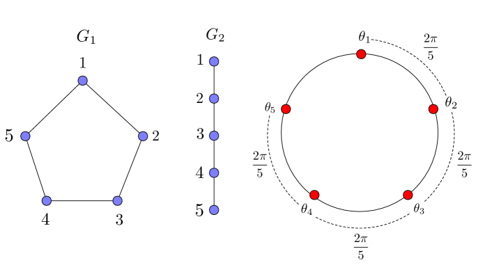
Example 9 (Comparing the three subsets).
Pick . In this example, we show that each of the inclusions in Theorem 8(i) is strict in general.
-
(i)
Consider a -cycle graph with the vector as shown in Figure 1. One can verify that , for every and therefore . However, using the embedding algorithm, it can be shown that .
-
(ii)
Consider an acyclic graph with nodes and the vector as shown in Figure 1. Then it is clear that . However, using the embedding algorithm, it can be shown that .
III-C Kuramoto map and its properties
We now define the Kuramoto map by
| (6) |
This map arises naturally from the Kuramoto model as follows. Recall that, given nodal variables and given the identification in Theorem 8(iv), the equilibrium equation (4) can be rewritten as
| (7) |
and can be interpreted as a nodal balance equation. If one left-multiplies this nodal balance equation by , then one obtains an edge balance equation
| (8) |
where can be interpreted as a collection of flows through each edge.
The following theorem studies the properties of the map and shows the equivalence between the nodal and edge balance equations; see Appendix C for the proof.
Theorem 10 (Basic properties of the Kuramoto map).
Consider the Kuramoto model (3), with the graph , incidence matrix , weight matrix , and natural frequencies . Define the Kuramoto map as in (6) and pick . Then the following statements hold:
- (i)
-
(ii)
the function is real analytic and one-to-one on ;
-
(iii)
if there exists a synchronization manifold , then it is unique and locally exponentially stable.
IV Sufficient conditions for synchronization
In this section, we present novel sufficient conditions for existence and uniqueness of the synchronization manifold for the Kuramoto model in the domain , for . We start with a useful definition.
Definition 11 (Minimum amplification factor for scaled projection).
Consider an undirected weighted connected graph with incidence matrix , weight matrix , and cutset projection matrix . For and , define
-
(i)
the domain ;
-
(ii)
for , the scaled cutset projection operator ; and
-
(iii)
the minimum amplification factor of the scaled cutset projection on by:
Note that is well-defined because is a continuous function over a compact set. The proof of the following lemma is given in Appendix D.
Lemma 12 (The minimum amplification factor is non-zero).
With the same notation and under the same assumptions as Definition 11, the minimum amplification factor of the scaled projection satisfies .
IV-A Main results
Now, we are ready to state the main results of this paper. We start with a family of general conditions for synchronization of Kuramoto model (3).
Theorem 13 (General sufficient conditions for synchronization).
Consider the Kuramoto model (3) with undirected weighted connected graph , the incidence matrix , the weight matrix , the cutset projection , and frequencies . For , if there exists such that
| (T1) |
then there exists a unique locally exponentially stable synchronization manifold for the Kuramoto model (3) in the domain .
Note that one can generalize test (T1) to the setting of arbitrary sub-multiplicative norms, with the caveat that the solution may take value outside .
Proof of Theorem 13.
We first show that, for every , we have . Suppose that . Then, by definition of , there exists such that and . Note that, for any vector , the -norm of is larger than or equal to the -norm of . This implies that . Therefore, by definition of , we obtain and, as a result, we have . Suppose that and . Then is a synchronization manifold for the Kuramoto model (3) if and only if
For every , define the map by
The following lemma, whose proof is given in Appendix E, studies some of the properties of the map .
Lemma 14.
For every , then the map is invertible and, for every ,
| (9) |
Now we get back to the proof of Theorem 13. For every and every define the map by
Note that by Lemma 14, we have
For every , we have . Therefore, by [37, Theorem 4.2], the map is continuous on . We first show that, if the assumption (T1) holds, then . Given , note the following inequality:
| (10) | ||||
Since is invertible, using Lemma 24 in Appendix D,
| (11) |
Combining the inequalities (10), (IV-A), and (T1), we obtain
In summary, is a continuous map from a compact convex set into itself. Therefore, by the Brouwer Fixed-Point Theorem, has a fixed-point in . Since, for every , we have , there exists such that . Therefore, we have
The fact that is the unique synchronization manifold of the Kuramoto model (3) in follows from Theorem 10 parts (i) and (iii). ∎
Theorem 13 presents a novel family of sufficient synchronization conditions for the Kuramoto model (3). However, these tests require the computation of the minimum amplification factor , that is, the solution to an optimization problem (see Definition 11) that is generally nonconvex. At this time we do not know of any reliable numerical method to compute for large dimensional systems. Therefore, in what follows, we focus on finding explicit lower bounds on , thereby obtaining computable synchronization tests.
Theorem 15 (Sufficient conditions for synchronization based on -norm).
Consider the Kuramoto model (3) with undirected unweighted connected graph , the incidence matrix , the cutset projection matrix , and frequencies . Then the following statements hold:
-
(i)
for every ,
-
(ii)
for every , if the following condition holds:
(T2) then there exists a unique locally exponentially stable synchronization manifold for the Kuramoto model (3) in the domain .
Proof.
First note that , for every . This implies that
| (12) |
Multiplying both sides of the inequality (12) by , we get
Note that , for every . Thus, [22, Corollary 7.7.4 (c)] implies
In turn this inequality implies
Now, Weyl’s Theorem [22, Theorem 4.3.1] implies
so that, for every ,
| (13) |
Regarding part (i), note that is an idempotent symmetric matrix. Thus, by setting , we have
Therefore, using (12) and (13), we get
This completes the proof of part (i). Regarding part (ii), if the assumption (T2) holds, then
The result follows by using the test (T1) for . ∎
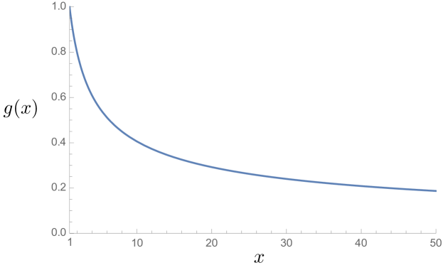
It is now convenient to introduce the smooth function defined by
| (14) |
One can verify that , is monotonically decreasing, and ; the graph of is shown in Figure 2.
Theorem 16 (Sufficient conditions for synchronization based on general lower bound).
Consider the Kuramoto model (3) with undirected weighted connected graph , the incidence matrix , the weight matrix , the cutset projection matrix , and frequencies . For , define the angle
| (15) |
Then the following statements hold:
-
(i)
for every , we have
-
(ii)
if the following condition holds:
(T3) then there exists a unique locally exponentially stable synchronization manifold for the Kuramoto model (3) in the domain .
Proof.
Regarding part (i), let . The triangle inequality implies that, for every and every with ,
| (16) |
Using triangle inequality, the last term in the inequality (16) can be upper bounded as
Moreover, the matrix is diagonal and by [22, Theorem 5.6.36], we have
Therefore, the inequality (16) can be rewritten as
By setting , we have
In turn , and we get
Part (i) of the theorem simply follows by taking the minimum over and such that .
Regarding part (ii), note that, by part (i), we have
Define the function by
Then one can compute:
| (17) | ||||
| (18) |
Using the equation (17), one can check that the unique critical point of in the interval is the solution to
This implies that is given as in equation (15). Moreover, we have
so that is a local maximum for . Now by using test (T1), if the following condition holds:
then there exists a unique locally exponentially stable synchronization manifold for the Kuramoto model (3) in the domain . Using the lower bound for given in part (i), it is easy to see that if the following condition holds:
then there exists a unique locally exponentially stable synchronization manifold for the Kuramoto model (3) in the domain . This completes the proof of the theorem. ∎
IV-B Comparison with previously-known synchronization results
IV-B1 General topology (-norm synchronization conditions)
To the best of our knowledge, sufficient conditions for synchronization of networks of oscillators with general topology was first studied in the paper [24]. Using the analysis methods introduced in [24], the tightest sufficient condition for synchronization of networks of oscillators with general topology [13, Theorem 4.7] can be obtained by the following test:
| (T0) |
where is the Fiedler eigenvalue of the Laplacian (see the survey [16] for more discussion). One can show that, for unweighted graphs test (T2) gives a sharper sufficient condition than test (T0). This fact is a consequence of the following lemma, whose proof is given in Appendix F.
Lemma 18.
Let be a connected, undirected, weighted graph with the incidence matrix and weight matrix . Assume that is the Laplacian of with eigenvalues . Then the following statements hold:
-
(i)
each satisfies the inequality
(19) with the equality sign if and only if belongs to the eigenspace associated to ; and
- (ii)
IV-B2 General topology (-norm synchronization conditions)
The approximate test was proposed in [17] as an approximately-correct sufficient condition for synchronization; statistical evidence on random graphs and IEEE test cases shows that the condition has much predictive power. However, [17] also identifies a family of counterexamples, where the condition is shown to be incorrect. Our test (T3) with is a rigorous, more conservative, and generically-applicable version of that approximately-correct test.
IV-B3 Acyclic topology
Consider the Kuramoto model (3) with acyclic connected graph and . Then the existence and uniqueness of synchronization manifolds of (3) in can be completely characterized by the following test [16, Corollary 7.5]:
| (20) |
We show that this characterization can be obtained from the general test (T1) for .
Corollary 19 (Synchronization for acyclic graphs).
Consider the Kuramoto model (3) with the acyclic undirected weighted connected graph , the incidence matrix , the weight matrix , and . Pick . Then the following conditions are equivalent:
-
(i)
,
-
(ii)
there exists a unique locally exponentially stable synchronization manifold for the Kuramoto model (3) in .
Additionally, if either of the above equivalent conditions holds, then the unique synchronization manifold in is .
Proof.
(i) (ii): Note that, for every and every such that , we have
In turn, this implies that
Therefore, by using the test (T1) for , there exists a unique locally stable synchronization manifold for the Kuramoto model (3).
(ii) (i): If there exists a unique locally stable synchronization manifold for the Kuramoto model (3) in , by Theorem 10(i), we have
Since and , we have and, in turn,
This completes the proof of equivalence of (i) and (ii). If is a synchronization manifold for the Kuramoto model (3) in , then we have . This implies that
Therefore, by pre-multiplying both side of the above equality into , we obtain
Thus, since , we get . This completes the proof of the theorem. ∎
IV-B4 Unweighted ring graphs and unweighted complete graphs
To the best of our knowledge, the sharpest sufficient condition for existence of a synchronization manifold in the domain for the Kuramoto model (3) with unweighted complete graph is given by the following test [16, Theorem 6.6]:
| (21) |
and for the Kuramoto model (3) with unweighted ring graph is given by the following test [17, Theorem 3, Condition 3]:
| (22) |
One can use the lower bound given in Theorem 16(i) to obtain another sufficient conditions for synchronization of unweighted complete and ring graphs.
Corollary 21 (Sufficient synchronization conditions for unweighted complete and ring graphs).
Consider the Kuramoto model (3) with either unweighted complete or unweighted ring graph , the incidence matrix , cutset projection , and . For every , define the scalar function by
| (23) |
If the following condition holds:
then there exists a unique locally stable synchronization manifold for the Kuramoto model (3) in
Proof.
By Theorem 5(iii) and (iv), the -norm of the cutset projection matrix for graph with nodes which is either unweighted complete or unweighted ring, is given by . Therefore, Theorem 16(i) implies the following lower bound:
| (24) |
Combining the bound on with the test (T1) for , we get the following test for the synchronization of unweighted complete graphs:
| (25) |
The proof of the corollary is complete by using Theorem 13. ∎
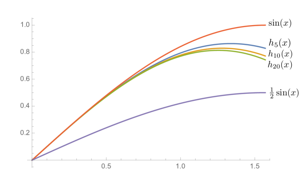
Note that, the function is positive and increasing on the interval . Therefore, for every and every , we have . Thus, for unweighted complete graphs, the test (25) is more conservative than the existing test (21). It is worth mentioning that the gap between the new test (25) and the existing test (21) decreases with the decrease of the angle . For instance, for , the right hand side of the test (25) asymptotically converges to . Therefore, at , the sufficient test (25) is approximately more conservative than the test (21). Instead, for , the right hand side of the test (25) asymptotically converges to . This means that, at , the test (25) is approximately more conservative than the test (21). The comparison between the graph of the functions , , and and over the interval is shown in Figure 3.
For unweighted ring graphs, it is easy to see that the sufficient condition (25) is always sharper than the existing sufficient condition (22). The comparison between the graph of the functions , , and and for is shown in Figure 3.
IV-B5 IEEE test cases
Here we consider various IEEE test cases described by a connected graph and a nodal admittance matrix . The set of nodes of is partitioned into a set of load buses and a set of generator buses . The voltage at the node is denoted by , where and the power demand (resp. power injection) at node (resp. ) is denoted by . By ignoring the resistances in the network, the synchronization manifold of the network satisfies the following Kuramoto model [17]:
| (26) |
where , for connected nodes and . For the nine IEEE test cases given in Table I, we numerically check the existence of a synchronization manifold for the Kuramoto model (26) in the domain . We consider effective power injections to be a scalar multiplication of nominal power injections, i.e., given nominal injections we set , for some and for every . The voltage magnitudes at the generator buses are pre-determined and the voltage magnitudes at load buses are computed by solving the reactive power balance equations using the optimal power flow solver provided by MATPOWER [47]. The critical coupling of the Kuramoto model (26) is denoted by and is computed using MATLAB fsolve. For a given test T, the smallest value of scaling factor for which the test T fails is denoted by . We define the critical ratio of the test T by . Intuitively speaking, the critical ratio shows the accuracy of the test T. Table I contains the following information:
- The first two columns
- The third column
-
gives the critical ratio for the following approximate test proposed in [17]:
(AT0) - The fourth column
-
gives the critical ratio for following approximate version of the test (T1):
(AT1) where is the approximate value for computed using MATLAB fmincon. Test (AT1) is approximate since, in general, fmincon may not converge to a solution and, even when it converges, the solution is only guaranteed to be an upper bound for .
| Test Case | Critical ratio | |||
|---|---|---|---|---|
| test | -norm test | Approx. test | General test | |
| (T0)[13] | (T3) | (AT0) [17] | (AT1) | |
| IEEE 9 | 16.54 | 73.74 | 92.13 | 85.06 † |
| IEEE 14 | 8.33 | 59.42 | 83.09 | 81.32 † |
| IEEE RTS 24 | 3.86 | 53.44 | 89.48 | 89.48 † |
| IEEE 30 | 2.70 | 55.70 | 85.54 | 85.54 † |
| IEEE 39 | 2.97 | 67.57 | 100 | 100 † |
| IEEE 57 | 0.36 | 40.69 | 84.67 | —* |
| IEEE 118 | 0.29 | 43.70 | 85.95 | —* |
| IEEE 300 | 0.20 | 40.33 | 99.80 | —* |
| Polish 2383 | 0.11 | 29.08 | 82.85 | —* |
-
•
† fmincon has been run for randomized initial phase angles.
-
•
* fmincon does not converge.
Note how (i) our ordering (T0) (T3) (AT0) is representative of the tests’ accuracy, (ii) our proposed test (T3) is two order of magnitude more accurate that best-known prior test (T0) in the larger test cases, (iii) the two approximate tests (AT0) and (AT1) are comparable (but our proposed test (AT1) is much more computationally complex).
V Conclusion
In this paper, we introduced and studied the cutset projection, as a geometric operator associated to a weighted undirected graph. This operator naturally appears in the study of networks of Kuramoto oscillators (3); using this operator, we obtained new families of sufficient conditions for network synchronization. For a network of Kuramoto oscillators with incidence matrix , Laplacian and frequencies , these sufficient conditions are in the form of upper bounds on the -norm of the edge flow quantity . In other words, our results highlight the important role of this edge flow quantity in the synchronization of Kuramoto oscillators. We show that our results significantly improve the existing sufficient conditions in the literature in general and, specifically, for a number of IEEE power network test cases.
Our approach and results suggest many future research directions. First, it is important to study the cutset projection in more detail and for more special cases. We envision that the cutset projection and its properties will be a valuable tool in the study of network flow systems, above and beyond the case of Kuramoto oscillators. Secondly, it is of interest to analyze and improve the accuracy of our sufficient conditions. This can be potentially done by designing efficient algorithm for numerical computation (or estimation) of the minimum amplification factor for large graphs. Thirdly, it is interesting to compare our new -norm tests, for different , and potentially extend them using more general norms. Finally, in power network applications, it is potentially of significance to generalize our novel approach to study the coupled power flow equations.
Acknowledgments
The authors thank Elizabeth Huang for her helpful comments, and Brian Johnson and Sairaj Dhople for wide-ranging discussions on power networks. The second author would also like to thank Florian Dörfler for countless conversations on Kuramoto oscillators.
Appendix A Proof of Theorems 4 and 5
We report here a useful well-known lemma, which is a simplified version of [7, Theorem 13].
Lemma 22 (Oblique projections).
For , assume the matrices satisfy . Then the oblique projection matrix onto parallel to is .
Proof of Theorem 4.
Regarding the statement (i), we first show that . Suppose that . Then there exists such that and
Since is connected, is a simple eigenvalue of the Laplacian associated to the eigenvector . This implies that and . Therefore, . Moreover, note that:
Therefore, as in statement (i).
Finally, statement (iii) is a known consequence of statements (ii) and (i). It is instructive, anyway, to provide an independent proof. Note the following equalities:
Using the fact that , we obtain . This implies that
Thus, the cutset projection is an idempotent matrix and its only eigenvalues are and [22, 1.1.P5]. ∎
Proof of Theorem 5.
Regarding part (i), when , we have . Moreover, for every , there exists such that . Therefore, for every ,
Moreover, we have . This implies that . Therefore, the projection is an orthogonal projection.
Regarding part (ii), since is acyclic, we have and . Now consider a vector . Since , there exists a unique such that . Therefore, we have
This implies that .
Appendix B Proof of Theorem 8
We start with a preliminary result.
Lemma 23.
Given , let be the output of the Embedding Algorithm with input . Then, for every two nodes , there exists a simple path in such that , , and
Proof.
It suffices to show that, for every there exists a simple path from the node to node such that, for every , we have
Start with node . Suppose that is being added to in the Embedding algorithm in the th iteration. For every , we denote the set in the th iteration of the Embedding algorithm by . Therefore but . Thus, by the algorithm, there exists such that . Now, we can repeat this procedure for to get such that . We can continue doing this procedure until we get to the node . Thus we get the simple path . ∎
We are now ready to provide the main proof of interest.
Proof of Theorem 8.
Regarding part (i), we first show the inclusion . Let . Then, by definition of , there exists and such that
This means that, for every , we have
Therefore, .
Now consider a point . By definition, there exists an arc of length on which contains . Since , this implies that there exists such that and, for every , we have
We define the vector by . Then it is clear that and . On the other hand, for every , the distance between and is the same as the distance between and . Therefore, we have
This implies that . Therefore, .
Regarding part (ii), using Lemma 23, it is a straightforward exercise to show that if , then we have , for some . This implies that .
Regarding part (iii), suppose that . Then we have . Since , it is clear that .
Now suppose that , we will show that . Assume that . Therefore, there exists such that . However, by the definition of the set , there exists such that and . This implies that . Thus, there exists a vector whose components are integers such that . Since we have and , we cannot have and . Therefore, and we have . However, by Lemma 23, since , there exists a simple path between the nodes and such that, for every , we have . Since and we have . Similarly, one can show that , for every . This implies that . However, this means that , which is a contradiction.
Regarding part (iv), we first show that the set is compact. Since , it suffice to show that it is closed and bounded. We first show that, for every , we have
where is the number of edges. Suppose that and for some we have . Since , we get
On the other hand, and is connected. Therefore, for every , there exists a simple path of length at most such that and . This implies that
Therefore, for every , we have . As a result, we get , which is a contradiction since and we have . Similarly, one can show that, for every , we have , for every . Therefore, is bounded. The closedness of the set is clear from continuity of the -norm. This implies that is compact. Now we define the map by . We show that is a real analytic diffeomorphism. It is easy to check that, for every , is an isomorphism. Therefore is local diffeomorphim for every . Now we show that is one-to-one on the set . Suppose that, for , we have . Therefore, we get , where is a vector whose components are integers. We will show that . Suppose that . Since graph is connected, there exists such that . This implies that
| (27) |
Since we have , we get . However, by equation (27), we have
However, this is a contradiction with the fact that . Therefore, and the map is one-to-one. Note that by part (iii), is also surjective. Therefore, using [29, Corollary 7.10], the map is a diffeomorphism between and . This completes the proof of part (iv). ∎
Appendix C Proof of Theorem 10
Regarding part (i), suppose that is a synchronization manifold for the Kuramoto model (7). Then . By left-multiplying both side of this equation by , we get
On the other hand, suppose that satisfies the edge balance equation (8). Then, if we left-multiply both side of this equation by , we get
Noting that and , we have
Moreover, we have and since , we get . This implies that . This completes the proof of part (i).
Appendix D Proof of Lemma 12 and of a useful equality
Proof of Lemma 12.
By definition of the minimum amplification factor, it is clear that, for every and every , we have . So, to prove the lemma, it suffices to show that, for every and every , we have . Suppose that for some and some , we have . Since and are compact sets, there exist and with the property that such that
By premultipling both side of the above equality by , we get . On the other hand, we know
where the last equality is a direct consequence of . This implies that . Since both and are diagonal positive definite matrices, we have . This is a contradiction with the fact that . ∎
The next result connects the minimum gain of an invertible operator with the norm of .
Lemma 24.
Let be a normed real vector space and be a bijective linear map. Then
Appendix E Proof of Lemma 14
For every , define the linear operator by
Let . Then there exists such that . This implies that
Since , we have . This implies that,
Therefore, we get
Since both and are linear operators on , we deduce that is invertible and, for every :
This completes the proof of the lemma.
Appendix F A useful result and proof of Lemma 18
Regarding part (i), Note that is real and symmetric. Therefore, using singular-value decomposition [22, Corollary 2.6.6], there exists an orthogonal matrix such that:
where are ordered eigenvalues of . Then, using [7, Chapter 6, §2, Corollary 1] the matrix has the following singular-value decomposition:
Since , there exists which satisfies . Therefore, we can write
Since we have
we obtain
Therefore,
| (30) | ||||
This concludes the proof of inequality. Regarding the equality, suppose that is the smallest positive integer such that . Note that, by the above analysis, the equality holds for if and only if
| (31) |
We define the diagonal matrix by
This implies that the equality (31) holds if and only if
| (32) |
Since , the equality (32) holds if and only if . However, we know that
where is the eigenvector associated to the eigenvalue . This completes the proof of part (i). Regrading part (ii), if satisfies test (T0), then we have . Therefore, by part (i), we have
This means that satisfies test (T2).
References
- [1] J. A. Acebrón, L. L. Bonilla, C. J. P. Vicente, F. Ritort, and R. Spigler. The Kuramoto model: A simple paradigm for synchronization phenomena. Reviews of Modern Physics, 77(1):137–185, 2005. doi:10.1103/RevModPhys.77.137.
- [2] D. Aeyels and J. A. Rogge. Existence of partial entrainment and stability of phase locking behavior of coupled oscillators. Progress of Theoretical Physics, 112(6):921–942, 2004. doi:10.1143/PTP.112.921.
- [3] N. Ainsworth and S. Grijalva. A structure-preserving model and sufficient condition for frequency synchronization of lossless droop inverter-based AC networks. IEEE Transactions on Power Systems, 28(4):4310–4319, 2013. doi:10.1109/TPWRS.2013.2257887.
- [4] A. Araposthatis, S. Sastry, and P. Varaiya. Analysis of power-flow equation. International Journal of Electrical Power & Energy Systems, 3(3):115–126, 1981. doi:10.1016/0142-0615(81)90017-X.
- [5] A. Arenas, A. Díaz-Guilera, J. Kurths, Y. Moreno, and C. Zhou. Synchronization in complex networks. Physics Reports, 469(3):93–153, 2008. doi:10.1016/j.physrep.2008.09.002.
- [6] M. Barahona and L. M. Pecora. Synchronization in small-world systems. Physical Review Letters, 89:054101, 2002. doi:10.1103/PhysRevLett.89.054101.
- [7] A. Ben-Israel and T. N. E. Greville. Generalized Inverses: Theory and Applications. Springer, 2 edition, 2003. doi:10.1007/b97366.
- [8] E. Brown, J. Moehlis, and P. Holmes. On the phase reduction and response dynamics of neural oscillator populations. Neural Computation, 16(4):673–715, 2004. doi:10.1162/089976604322860668.
- [9] F. Bullo. Lectures on Network Systems. CreateSpace, 1 edition, 2018. With contributions by J. Cortés, F. Dörfler, and S. Martínez. URL: http://motion.me.ucsb.edu/book-lns.
- [10] M. C. Chandorkar, D. M. Divan, and R. Adapa. Control of parallel connected inverters in standalone AC supply systems. IEEE Transactions on Industry Applications, 29(1):136–143, 1993. doi:10.1109/28.195899.
- [11] N. Chopra and M. W. Spong. On exponential synchronization of Kuramoto oscillators. IEEE Transactions on Automatic Control, 54(2):353–357, 2009. doi:10.1109/TAC.2008.2007884.
- [12] F. Dörfler and F. Bullo. On the critical coupling for Kuramoto oscillators. SIAM Journal on Applied Dynamical Systems, 10(3):1070–1099, 2011. doi:10.1137/10081530X.
- [13] F. Dörfler and F. Bullo. Exploring synchronization in complex oscillator networks. In IEEE Conf. on Decision and Control, pages 7157–7170, Maui, USA, December 2012. doi:10.1109/CDC.2012.6425823.
- [14] F. Dörfler and F. Bullo. Synchronization and transient stability in power networks and non-uniform Kuramoto oscillators. SIAM Journal on Control and Optimization, 50(3):1616–1642, 2012. doi:10.1137/110851584.
- [15] F. Dörfler and F. Bullo. Kron reduction of graphs with applications to electrical networks. IEEE Transactions on Circuits and Systems I: Regular Papers, 60(1):150–163, 2013. doi:10.1109/TCSI.2012.2215780.
- [16] F. Dörfler and F. Bullo. Synchronization in complex networks of phase oscillators: A survey. Automatica, 50(6):1539–1564, 2014. doi:10.1016/j.automatica.2014.04.012.
- [17] F. Dörfler, M. Chertkov, and F. Bullo. Synchronization in complex oscillator networks and smart grids. Proceedings of the National Academy of Sciences, 110(6):2005–2010, 2013. doi:10.1073/pnas.1212134110.
- [18] G. B. Ermentrout. Synchronization in a pool of mutually coupled oscillators with random frequencies. Journal of Mathematical Biology, 22(1):1–9, 1985. doi:10.1007/BF00276542.
- [19] A. Franci, A. Chaillet, and W. Pasillas-Lépine. Phase-locking between Kuramoto oscillators: Robustness to time-varying natural frequencies. In IEEE Conf. on Decision and Control, pages 1587–1592, Atlanta, USA, December 2010. doi:10.1109/CDC.2010.5717876.
- [20] A. Ghosh, S. Boyd, and A. Saberi. Minimizing effective resistance of a graph. SIAM Review, 50(1):37–66, 2008. doi:10.1137/050645452.
- [21] C. D. Godsil and G. F. Royle. Algebraic Graph Theory. Springer, 2001.
- [22] R. A. Horn and C. R. Johnson. Matrix Analysis. Cambridge University Press, 2nd edition, 2012.
- [23] I. C. F. Ipsen and C. D. Meyer. The angle between complementary subspaces. American Mathematical Monthly, 102(10):904–911, 1995. doi:10.2307/2975268.
- [24] A. Jadbabaie, N. Motee, and M. Barahona. On the stability of the Kuramoto model of coupled nonlinear oscillators. In American Control Conference, pages 4296–4301, Boston, USA, June 2004. doi:10.23919/ACC.2004.1383983.
- [25] G. Jongen, J. Anemüller, D. Bollé, A. C. C. Coolen, and C. Perez-Vicente. Coupled dynamics of fast spins and slow exchange interactions in the XY spin glass. Journal of Physics A: Mathematical and General, 34(19):3957–3984, 2001. doi:10.1088/0305-4470/34/19/302.
- [26] I. Z. Kiss, Y. Zhai, and J. L. Hudson. Emerging coherence in a population of chemical oscillators. Science, 296(5573):1676–1678, 2002. doi:10.1126/science.1070757.
- [27] Y. Kuramoto. Chemical Oscillations, Waves, and Turbulence. Springer, 1984.
- [28] J. Lavaei and S. H. Low. Zero duality gap in optimal power flow problem. IEEE Transactions on Power Systems, 27(1):92–107, 2012. doi:10.1109/TPWRS.2011.2160974.
- [29] J. M. Lee. Introduction to Smooth Manifolds. Springer, 2003.
- [30] E. Mallada, R. A. Freeman, and A. K. Tang. Distributed synchronization of heterogeneous oscillators on networks with arbitrary topology. IEEE Transactions on Control of Network Systems, 3(1):1–12, 2016. doi:10.1109/TCNS.2015.2428371.
- [31] D. C. Michaels, E. P. Matyas, and J. Jalife. Mechanisms of sinoatrial pacemaker synchronization: A new hypothesis. Circulation Research, 61(5):704–714, 1987. doi:10.1161/01.RES.61.5.704.
- [32] R. E. Mirollo and S. H. Strogatz. The spectrum of the locked state for the Kuramoto model of coupled oscillators. Physica D: Nonlinear Phenomena, 205(1-4):249–266, 2005. doi:10.1016/j.physd.2005.01.017.
- [33] P. Monzón and F. Paganini. Global considerations on the Kuramoto model of sinusoidally coupled oscillators. In IEEE Conf. on Decision and Control, pages 3923–3928, San Diego, USA, December 2005. doi:10.1109/CDC.2005.1582774.
- [34] Y. Moreno and A. F. Pacheco. Synchronization of Kuramoto oscillators in scale-free networks. Europhysics Letters, 68(4):603, 2004. doi:10.1209/epl/i2004-10238-x.
- [35] T. Nishikawa, A. E. Motter, Y. C. Lai, and F. C. Hoppensteadt. Heterogeneity in oscillator networks: Are smaller worlds easier to synchronize? Physical Review Letters, 91(1):14101, 2003. doi:10.1103/PhysRevLett.91.014101.
- [36] J. Pantaleone. Stability of incoherence in an isotropic gas of oscillating neutrinos. Physical Review D, 58(7):073002, 1998. doi:10.1103/PhysRevD.58.073002.
- [37] V. Rakočević. On continuity of the Moore-Penrose and Drazin inverses. Matematicki Vesnik, 49(3-4):163–172, 1997. URL: http://www.emis.de/journals/MV/9734.
- [38] G. S. Schmidt, A. Papachristodoulou, U. Münz, and F. Allgöwer. Frequency synchronization and phase agreement in Kuramoto oscillator networks with delays. Automatica, 48(12):3008–3017, 2012. doi:10.1016/j.automatica.2012.08.013.
- [39] R. Sepulchre, D. A. Paley, and N. E. Leonard. Stabilization of planar collective motion: All-to-all communication. IEEE Transactions on Automatic Control, 52(5):811–824, 2007. doi:10.1109/TAC.2007.898077.
- [40] J. W. Simpson-Porco, F. Dörfler, and F. Bullo. Synchronization and power sharing for droop-controlled inverters in islanded microgrids. Automatica, 49(9):2603–2611, 2013. doi:10.1016/j.automatica.2013.05.018.
- [41] P. A. Tass. A model of desynchronizing deep brain stimulation with a demand-controlled coordinated reset of neural subpopulations. Biological Cybernetics, 89(2):81–88, 2003. doi:10.1007/s00422-003-0425-7.
- [42] M. Verwoerd and O. Mason. Global phase-locking in finite populations of phase-coupled oscillators. SIAM Journal on Applied Dynamical Systems, 7(1):134–160, 2008. doi:10.1137/070686858.
- [43] M. Verwoerd and O. Mason. On computing the critical coupling coefficient for the Kuramoto model on a complete bipartite graph. SIAM Journal on Applied Dynamical Systems, 8(1):417–453, 2009. doi:10.1137/080725726.
- [44] Y. Wang and F. J. Doyle III. Exponential synchronization rate of Kuramoto oscillators in the presence of a pacemaker. IEEE Transactions on Automatic Control, 58(4):989–994, 2013. doi:10.1109/TAC.2012.2215772.
- [45] N. Wiener. Nonlinear Problems in Random Theory. MIT Press, 1958.
- [46] A. T. Winfree. Biological rhythms and the behavior of populations of coupled oscillators. Journal of Theoretical Biology, 16(1):15–42, 1967. doi:10.1016/0022-5193(67)90051-3.
- [47] R. D. Zimmerman, C. E. Murillo-Sánchez, and R. J. Thomas. MATPOWER: Steady-state operations, planning, and analysis tools for power systems research and education. IEEE Transactions on Power Systems, 26(1):12–19, 2011. doi:10.1109/TPWRS.2010.2051168.
![[Uncaptioned image]](/html/1711.03711/assets/Author_SaberJafarpour2.jpg) |
Saber Jafarpour (M’16) is a Postdoctoral researcher with the Mechanical Engineering Department and the Center for Control, Dynamical Systems and Computation at the University of California, Santa Barbara. He received his Ph.D. in 2016 from the Department of Mathematics and Statistics at Queen’s University. His research interests include analysis of network systems with application to power grids and geometric control theory. |
![[Uncaptioned image]](/html/1711.03711/assets/fb-19sep14.jpg) |
Francesco Bullo (IEEE S’95-M’99-SM’03-F’10) is a Professor with the Mechanical Engineering Department and the Center for Control, Dynamical Systems and Computation at the University of California, Santa Barbara. He was previously associated with the University of Padova, the California Institute of Technology, and the University of Illinois. His research interests focus on network systems and distributed control with application to robotic coordination, power grids and social networks. He is the coauthor of “Geometric Control of Mechanical Systems” (Springer, 2004) and “Distributed Control of Robotic Networks” (Princeton, 2009); his forthcoming ”Lectures on Network Systems” is available on his website. He received best paper awards for his work in IEEE Control Systems, Automatica, SIAM Journal on Control and Optimization, IEEE Transactions on Circuits and Systems, and IEEE Transactions on Control of Network Systems. He is a Fellow of IEEE and IFAC. He has served on the editorial boards of IEEE, SIAM, and ESAIM journals, and serves as 2018 IEEE CSS President. |