Valuing the anticipative information on the stochastic short interest rates

Abstract

Portfolio optimization is an important financial tool in particular to price financial derivatives. However the standard techniques do not apply when it is needed to extend the model by including insight information and one has to recur to more sophisticated tools such as the enlargement of filtrations.

We show how to apply this technique to value the anticipative information about the short interest rate. We model the short rates by an affine diffusion process and compute the optimal portfolio for a large class of insight information and different utility functions. We conclude with a more detailed analysis of the Vasicek model and with some numerical examples.

Keywords— Stochastic programming; Optimal portfolio; Enlargement of filtrations; Vasicek interest rate model; Value of the information.

1 Introduction

We work within the framework of the optimal portfolio problem in an incomplete market in which an investing agent holds some anticipative information. In the literature the additional information commonly refers to the future trend of some trading asset, while in this work the focus is on the special case when the anticipative information refers to the future trend of the short interest rate. This situation creates an asymmetry in the market and we assume that there are two agents, one possessing the additional information and the other with the usual one.

The extension of the optimal portfolio problem to the case of anticipative information is generally dealt with the technique of enlargement of filtrations by which a new filtration containing the anticipative information is created. In order to assure that in the new filtration all the previously martingales are preserved at least as semimartingales, it is assumed that the new information satisfies the so-called Jacod’s hypothesis, see Assumption 2.2 below.

A first type of enlargement of filtration – the one dealt with in this paper – is the so-called initial enlargement, where the additional information is revealed to the informed agent since the beginning. This procedure was originally applied to the optimal portfolio problem in [1]. They assume that the anticipative information is modeled by a random variable satisfying the Jacod’s hypothesis and they explicitly solve for the optimal investment strategy in a variety of examples. In [2] it is shown that the value of the additional information, measured by mean of the expected logarithmic utility, is equal to its entropy when it is represented by an atomic random variable. They also show that whenever this random variable is not purely atomic, the additional gain is always unbounded. In [3], the optimal portfolio problem is solved for utility functions different from the logarithmic (CRRA and exponential). The price of the information is introduced as the fair price that an investor should pay at the beginning to acquire the additional information. In [4], the Jacod’s hypothesis is weakened by solving the optimal portfolio problem via the Malliavin calculus, while in [5], it is discussed the relationship between owning additional information and the financial opportunities of arbitrage. Computing the value of the additional information is an active topic of research as shown by recent results such as [6], where the authors quantify in a general semimartingale context the value of arbitrage opportunities, and [7], where the authors analyze the value of the information related to the jumps of a Poisson process.

Another type of enlargement of filtration, that it is not considered in this work, but that we mention because it has recently attracted a lot of interest in the literature, is the progressive enlargement, where the information is represented by a random time that is made a stopping time in the enlarged filtration. We refer the reader to [8] and the references therein for a recent survey. We also mention [9] that introduces an additional type of enlargement via a stochastic process, and [10] that shows an alternative technique to deal with anticipative information by applying a stochastic maximum principle.

In general, all the above mentioned references assume that the additional information refers directly to some traded assets, while in this work we focus on the case where the information refers to the stochastic interest rate. Incidentally, this problem was stated in [1] as open. Our aim is to compute the expected utility gain that an agent could get in the situation she knows some information about the future value of the interest rate.

We assume as model for the interest rate a general affine diffusion process, as this structure is quite flexible and allows in many cases to get quite explicit expressions. Moreover this class includes, as a special case, the Ornstein-Uhlenbeck process that allows to analyze in very detail the well-known Vasicek model, introduced in [11]. Note that this interest rate process can reach negative values with positive probability. Some authors try to modify this situation in several ways, for example see [12]. However, we employ the usual Vasicek model in order to simplify the computations involving the distribution of the process. The stochastic interest rate creates incompleteness in the market, just as it occurs in [13], although in that reference it is due to sudden jumps in the interest rate and in this paper it is due to its source of randomness.

We compute the optimal utility for the non-discounted wealth in an initial enlargement setting and give an explicit equation for the optimal strategy. We do this for different types of utility functions (logarithmic, CRRA and exponential), and by assuming that the information is of linear type (see Section 4). Except for the logarithmic utility, cfr. Examples 3.12 and 3.13, the optimal strategy is given in implicit form because the classical Merton argument does not work as was already noticed [14]. Incidentally we also explicitly compute the predictable representation property of some special random variables and solve some stochastic integrals that cannot be handled with usual techniques.

The paper is organized as follows. In Section 2 we introduce in more detail the general model with the interest rate process modeled as an affine diffusion and we state the mathematical notation. In Section 3 we solve the utility maximization problem in the incomplete market. In Section 4 we analyze the interest rate process under the enlarged filtration with an integral-type random variable. We compute explicitly the semimartingale decomposition and the optimal utility expectation for non-discounted prices. In Section 5 we introduce a weaker type of information by assuming known at first a lower bound for the final value of the interest rate and then also an upper bound. Finally, we present an example in which the (NFLVR) is preserved within the enlarged filtration satisfying only the Jacod hypothesis of absolutely continuity in $[0,T]$ and the equivalence in $[0,T)$. In Section 6 we present some numerical examples and finally in Section 7 we end with some concluding remarks.

2 Model and Notation

As a general set-up we assume to work in a probability space $(\Omega,\mathcal{F},\mathbb{F},\boldsymbol{P})$ where $\mathcal{F}$ is the event sigma-algebra, and $\mathbb{F}=\{\mathcal{F}_{t},t\geq 0\}$ is an augmented filtration that is generated by the natural filtration of $(B^{R},B^{S})=((B^{R}_{t},B^{S}_{t}),t\geq 0)$, that is a bi-dimensional process whose components have constant correlation $\rho\neq 0$ and each one is an $\mathbb{F}$-Brownian motion. Sometimes we use the notation $\mathbb{F}^{R}$ ($\mathcal{F}_{T}^{R}$) to denote the filtration (sigma-algebra) generated by the process $B^{R}$. We also fix a finite horizon time $T>0$ in which the trader could invest.

To simplify our analysis we consider a simple portfolio made of only two assets, one risky, $S=(S_{t},\,0\leq{t}\leq{T})$, and the other riskless, $D=(D_{t},\,0\leq{t}\leq{T})$, and both processes are adapted semimartingales in the defined probability space. In particular their dynamics are defined by the following SDEs,

$$dD_{t} =D_{t}\,R_{t}\,dt\ ,\quad D_{0}=1$$ (2.1a)

$$dS_{t} =S_{t}\,\left(\eta_{t}dt+\xi_{t}dB^{S}_{t}\right)\ ,\ \,\quad S_{0}=s_{0}>0$$ (2.1b)

where $R=(R_{t},\,0\leq{t}\leq{T})$ is the instantaneous interest rate, sometimes also called the short term rate. The drift and the volatility of the risky asset are given by the processes $\eta=(\eta_{t},\,0\leq{t}\leq{T})$ and $\xi=(\xi_{t},\,0\leq{t}\leq{T})$, which are assumed to be predictable to the natural filtration $\mathbb{F}$ and satisfying the following condition

$$\boldsymbol{E}\left[\int_{0}^{T}\left(\frac{\eta_{t}-R_{t}}{\xi_{t}}\right)^{2}dt\right]<+\infty\ .$$

We assume that the process $1/\xi$ is bounded. The interest rate process $R$ is assumed to be an affine diffusion, satisfying the following SDE,

$$dR_{t}=\left[a_{1}(t)R_{t}+a_{2}(t)\right]dt+b_{2}(t)dB^{R}_{t}\ ,\quad R_{0}=r_{0}>0\ ,$$ (2.2)

where the deterministic functions $a_{1},a_{2},b_{2}$ are sufficiently smooth. Note that the market is incomplete because there is only one tradeable asset while there are two sources of randomness $(B^{R},B^{S})$. This class of processes includes as a particular case the Ornstein-Uhlenbeck process, in this paper denoted by $Y=(Y_{t},\,0\leq{t}\leq{T})$. It satisfies the well-known SDE

$$dY_{t}=k(\mu-Y_{t})dt+\sigma dB^{Y}_{t}\ ,\quad Y_{0}=y_{0}>0\ ,$$ (2.3)

with $k,\mu,\sigma$ given parameters satisfying some conditions. Since its introduction in [11], it is often used to model the interest rate for its mean reverting property.

Under the above hypothesis we assume that an investor employs an admissible strategy $\pi=(\pi_{t},\,0\leq{t}\leq{T})$ with the aim to optimize a given utility function at a finite terminal time $T>0$.

Definition 2.1.

We define the set of admissible strategies $\mathcal{A}(\mathbb{H})$ which contains all the self-financing portfolios $\pi=(\pi_{t},\,0\leq{t}\leq{T})$ such that,

• $\pi$ is adapted with respect to the filtration $\mathbb{H}$

• $\int_{0}^{T}\xi_{t}^{2}\pi_{t}^{2}dt<+\infty$, $\boldsymbol{P}$-almost surely

where $\pi_{t}$ is the proportion of the capital invested in the risky asset at time t.

Denoting by $X^{\pi}=(X^{\pi}_{t},\,0\leq{t}\leq{T})$ the wealth of the portfolio of the investor under an admissible strategy $\pi$, we can write its dynamics as the solution of the following SDE, for $0\leq t\leq T$,

$$\frac{dX_{t}^{\pi}}{X_{t}^{\pi}} =(1-\pi_{t})\frac{dD_{t}}{D_{t}}+\pi_{t}\frac{dS_{t}}{S_{t}}\ ,\quad X_{0}=x_{0}>0\ .$$

Using (2.1), it can be expressed in the following form

$$dX_{t}^{\pi} =(1-\pi_{t})X_{t}^{\pi}R_{t}\,dt+\pi_{t}X_{t}^{\pi}\left(\eta_{t}\,dt+\xi_{t}\,dB^{S}_{t}\right)\ ,\quad X_{0}=x_{0}\ .$$ (2.4)

Usually it is assumed that the strategy $\pi$ makes optimal use of all information at disposal of the agent at each instant, and in general we are going to assume that the agent’s flow of information, modeled by the filtration $\mathbb{H}=(\mathcal{H}_{t},\,0\leq{t}\leq{T})$, is possibly larger than filtration $\mathbb{F}$, that is $\mathbb{F}\subset\mathbb{H}$. We define the optimal portfolio $\pi^{\mathbb{H}}=(\pi^{\mathbb{H}}_{t},\,0\leq{t}\leq{T})$ as the solution of the following optimization problem,

$$\mathbb{V}_{T}^{\mathbb{H}}\coloneqq\sup_{\pi\in\mathcal{A}({\mathbb{H}})}\boldsymbol{E}[U(X^{\pi}_{T})]=\boldsymbol{E}\left[U\left(X^{\pi^{\mathbb{H}}}_{T}\right)\right]\ ,$$ (2.5)

where $\mathbb{V}_{T}^{\mathbb{H}}$ is defined as the optimal value of the portfolio at time $T$ given the information flow $\mathbb{H}$. The function $U:\mathbb{R}^{+}\rightarrow\mathbb{R}$ denotes the utility function and it is assumed to be continuous, increasing and concave in its domain and satisfying $U(x)=-\infty$ for $x<0$. In addition we assume that it is continuously differentiable, being $U^{\prime}$ strictly increasing and strictly concave in its domain and satisfying the Inada conditions,

$$U^{\prime}(0) :=\lim_{x\to 0^{+}}U^{\prime}(x)=+\infty$$ (2.6a)

$$U^{\prime}(+\infty) :=\lim_{x\to\infty}U^{\prime}(x)=0\ .$$ (2.6b)

In order to analyze enlarged information flows, in the following sections we consider some examples of initial enlargements constructed from the addition of a random variable $G$ measurable in the sigma-algebra $\mathcal{F}_{T}$. We define the enlarged filtration $\mathbb{G}=\{\mathcal{G}_{t},t\geq 0\}$ as follows,

$$\mathcal{G}_{t}=\bigcap_{s>t}\left(\mathcal{F}_{s}\vee\sigma(G)\right)\ .$$ (2.7)

In short, we will write $\mathbb{G}$ as the minimum filtration which is right-continuous and contains $\mathbb{F}\vee\sigma(G)$. In our paper, as a result of the asymmetry produced by the knowledge of the random variable $G$, we will assume that there exists a $\mathbb{G}$-agent, informed of $G$ since the beginning, and an $\mathbb{F}$-agent who plays with the natural information flow $\mathbb{F}$.

Our results rely on the following assumption usually known in the literature as the Jacod’s hypothesis.

Assumption 2.2 (Jacod’s hypothesis).

The distribution of the random variable $G$ is $\sigma$-finite while the regular $\mathcal{F}_{t}$-conditional distributions verify the equivalent condition $\boldsymbol{P}(G\in\cdot|\mathcal{F}_{t})\ll\,\boldsymbol{P}(G\in\cdot)$, $\boldsymbol{P}$-almost surely for $t\in[0,T)$.

This assumption assures the existence of a jointly measurable $\mathbb{F}$-adaptedprocess denoted by $p^{g}=(p^{g}_{t},\,0\leq{t}<T)$, with $g\in Supp(G)$, and such that$\boldsymbol{P}(A|\mathcal{F}_{t})=\int_{A}p^{g}_{t}\boldsymbol{P}(G\in dg)$ for any $A\in\sigma(G)$. In particular,

$$p_{t}^{g}=\frac{\boldsymbol{P}(G\in dg|\mathcal{F}_{t})}{\boldsymbol{P}(G\in dg)}\ ,\quad 0\leq t<T\ .$$

The following proposition allows to compute the $\mathbb{G}$-semimartingale decomposition of any $\mathbb{F}$-continuous local martingale, it was stated originally in [15, Theorem 2.1]. The process $p^{g}$, for any $g\in Supp(G)$, is an $\mathbb{F}$-martingale, see [2, Lemma 2.1], and therefore $\langle X,p^{g}\rangle^{\mathbb{F}}=(\langle X,p^{g}\rangle^{\mathbb{F}}_{t},\,0\leq{t}<T)$ is well-defined for any $\mathbb{F}$-local martingale $X$. Moreover, we define

$$\langle X,p^{G}\rangle_{s}^{\mathbb{F}}:=\langle X,p^{\cdot}\rangle_{s}^{\mathbb{F}}\circ G\ .$$

Proposition 2.3.

Let $X=(X_{t},\,0\leq{t}\leq{T})$ be an $\mathbb{F}$-continuous local martingale and let $G$ be an $\mathcal{F}_{T}$-measurable random variable satisfying the Jacod’s hypothesis. Then, the process

$$\widehat{X}_{t}=X_{t}-\int_{0}^{t}\frac{d\langle X,p^{G}\rangle_{s}^{\mathbb{F}}}{p^{G}_{s-}}\ ,\quad 0\leq t<T\$$ (2.8)

is a $\mathbb{G}$-local martingale.

When the compensator of the process $X$ appearing in (2.8) is absolutely continuous with respect to the Lebesgue measure, its density is usually called the information drift and it plays a crucial role in our computations. We will use the notation $\alpha^{G}=(\alpha^{G}_{t},\,0\leq{t}<T)$ for the information drift related to the process $B^{R}$, i.e.,

$$\int_{0}^{t}\alpha^{G}_{s}ds:=\int_{0}^{t}\frac{d\langle B^{R},p^{G}\rangle_{s}^{\mathbb{F}}}{p^{G}_{s-}}\ ,\quad 0\leq t<T\ ,$$

see Proposition 4.4 for more details.

Although the opportunities of arbitrage are not a central issue in our paper, we mention a result that links the Novikov’s condition on $\alpha^{G}$ with the No Free Lunch Vanishing Risk (NFLVR) condition in the enlarged filtration for $G\in\mathcal{F}_{T}^{R}$. A simple proof can be found in [16] and we refer to [17] for a general background about the arbitrage theory.

Proposition 2.4.

With the previous set-up, if $G\in\mathcal{F}_{T}^{R}$ and the process $\alpha^{G}$ satisfies

$$\boldsymbol{E}\left[\exp\left(\frac{1}{2}\int_{0}^{T}(\alpha_{t}^{G})^{2}dt\right)\right]<+\infty\ ,$$ (2.9)

then the (NFLVR) condition within $\mathbb{G}$ holds true.

2.1 Additional Notation

Given two random variables $X$ and $Y$, we write $X\approx Y$ to indicate that they have the same distribution. The notation $\mathcal{N}(\mu,\sigma^{2})$ denotes a Gaussian random variable with mean $\mu$ and variance $\sigma^{2}$. $\Phi(z)$ denotes the cumulative distribution of a standard Gaussian random variable. With $f_{X}(x)$ we denote the density function of $X$ evaluated at $x$ and by $f_{X|Y}(x|y)$ the value of the conditioned density function at $x$ given $\{Y=y\}$. $\boldsymbol{P}$ and $\boldsymbol{V}$ denote the probability and the variance operators. By $\boldsymbol{E}$ we mean the expectation operator under $\boldsymbol{P}$, i.e., $\boldsymbol{E}=\boldsymbol{E}_{\boldsymbol{P}}$. If we consider the expectation under another measure, for example $\boldsymbol{Q}$, we will specify as $\boldsymbol{E}_{\boldsymbol{Q}}$. If $\mathcal{H}$ is a $\sigma$-algebra, then with $\boldsymbol{E}[\cdot|\mathcal{H}]$ and $\boldsymbol{V}[\cdot|\mathcal{H}]$ we denote the conditional expectation and the conditional variance operators. We define the space $L^{2}(\Omega,\mathcal{H},\boldsymbol{P})$, or simply $L^{2}(\boldsymbol{P})$ when $(\Omega,\mathcal{H})$ is clear, the set of $\mathcal{H}$-measurable random variables $F$ with $\boldsymbol{E}[F^{2}]<+\infty$, i.e.,

$$L^{2}(\boldsymbol{P})=\{F:\boldsymbol{E}[F^{2}]<+\infty\}\ .$$

We define $L^{2}(J,\mathcal{H},dt\times\boldsymbol{P},\mathbb{H})$, or simply $L^{2}(J,dt\times\boldsymbol{P},\mathbb{H})$, as the space of all $\mathbb{H}$-adapted processes with the following integrability condition,

$$L^{2}(J,dt\times\boldsymbol{P},\mathbb{H})=\Big{\{}X=(X_{t},\,t\in J):\int_{J}\boldsymbol{E}\left[X_{s}^{2}\right]ds<+\infty\Big{\}}\ ,$$

and we simply write $L^{2}(dt\times\boldsymbol{P},\mathbb{H})$ when $J=[0,T]$. $(fg)(x)$ is sometimes used to denote the product $f(x)g(x)$.

3 Optimization Problem

Combining equations (2.2) and (2.4) we get the following system of stochastic differential equations,

$$\left\{\begin{aligned} dX_{t}^{\pi}&=(1-\pi_{t})X_{t}^{\pi}R_{t}\,dt+\pi_{t}X_{t}^{\pi}\left(\eta_{t}\,dt+\xi_{t}\,dB_{t}^{S}\right)\\ dR_{t}&=\left[a_{1}(t)R_{t}+a_{2}(t)\right]dt+b_{2}(t)dB^{R}_{t}\\ \end{aligned}\right.$$ (3.1)

that solved with respect to the filtration $\mathbb{F}$ gives the evolution of the interest rate process and the portfolio wealth, as seen by an $\mathbb{F}$-agent. To analyze the same processes adapted to the enlarged filtration $\mathbb{G}$ defined in (2.7), we employ standard techniques of enlargement of filtrations by looking for the $\mathbb{G}$-semimartingale decomposition of the pair $(B^{R},B^{S})$. The new representation is obtained in Proposition 3.2.

Assuming integrability for the functions $a_{1}$, $a_{2}$, and $b_{2}$ in (2.2) it is easy to see by applying Itô lemma, [18, Example 1.5.4.8] could be consulted, that the process $R$ admits the following explicit solution

$$R_{t} =\Psi_{t}\left[R_{0}+\int_{0}^{t}(a_{2}\Psi^{-1})(x)\,dx+\int_{0}^{t}(b_{2}\Psi^{-1})(x)\,dB^{R}_{x}\right]\ ,\quad 0\leq t\leq T\ ,$$ (3.2)

where $\Psi_{t}:=\exp\left({\int_{0}^{t}a_{1}(x)dx}\right)$ and $\Psi_{s,t}:=\exp\left({\int_{s}^{t}a_{1}(x)dx}\right)$. Sometimes, we will use the notation $\Psi(t):=\Psi_{t}$ when $\Psi^{-1}$ is involved. The process $R$ is Markov and Gaussian when $R_{0}$ is Gaussian distributed. Given that $R$ is a Markov process, we start by studying the distribution of $(R_{s}|R_{u})$ for $0\leq u\leq s$. We can calculate it by conveniently handling the explicit expression in (3.2) as we show in the following lemma.

Lemma 3.1.

Let $R$ be the process defined by (2.2). For $0\leq u\leq s$, the conditioned random variable $(R_{s}|R_{u})$ has the following distribution

$$(R_{s}|R_{u})\approx\mathcal{N}\left(\Psi_{u,s}R_{u}+\Psi_{s}\int_{u}^{s}\left(a_{2}\Psi^{-1}\right)(x)dx,\ \Psi_{s}^{2}\int_{u}^{s}\left(b_{2}\Psi^{-1}\right)^{2}(x)dx\right)\ .$$

Proof.

Using equation (3.2), we can express the value of $R_{s}$ in terms of its value at time $u$ in the following way,

$$R_{s} =\Psi_{u}\Psi_{u,s}\Big{[}R_{0}+\int_{0}^{u}\left(a_{2}\Psi^{-1}\right)(x)dx+\int_{u}^{s}\left(a_{2}\Psi^{-1}\right)(x)dx$$

$$\hskip 54.00009pt+\int_{0}^{u}\left(b_{2}\Psi^{-1}\right)(x)dB^{R}_{x}+\int_{u}^{s}\left(b_{2}\Psi^{-1}\right)(x)dB^{R}_{x}\Big{]}$$

$$=\Psi_{u,s}R_{u}+\Psi_{s}\left[\int_{u}^{s}\left(a_{2}\Psi^{-1}\right)(x)dx+\int_{u}^{s}\left(b_{2}\Psi^{-1}\right)(x)dB^{R}_{x}\right]\ .$$ (3.3)

The result then follows by identifying the deterministic and stochastic part of formula (3), the latter gives the variance by applying the Itô isometry. ∎

3.1 Optimal Portfolio

The analysis above allows to rewrite the SDE (3.1), expressed in the filtration $\mathbb{F}$, under the filtration $\mathbb{G}$ as shown by the following proposition.

Proposition 3.2.

Under the filtration $\mathbb{G}$ the processes $X^{\pi}=(X^{\pi}_{t},\,0\leq{t}<T)$ and $R=(R_{t},\,0\leq{t}\leq{T})$ satisfy the following SDE:

$$\left\{\begin{aligned} dX_{t}^{\pi}&=(1-\pi_{t})X_{t}^{\pi}R_{t}\,dt+\pi_{t}X_{t}^{\pi}(\eta_{t}dt+\xi_{t}dB_{t}^{S})\\ dR_{t}&=\left[a_{1}(t)R_{t}+\left(a_{2}(t)+b_{2}(t)\alpha_{t}^{G}\right)\right]\,dt+b_{2}(t)dW_{t}^{R}\\ dB_{t}^{S}&=\rho\alpha_{t}^{G}\,dt+\rho dW_{t}^{R}+\sqrt{1-\rho^{2}}dB_{t}\ ,\quad 0\leq t<T\ .\end{aligned}\right.$$ (3.4)

Where $W^{R}=(W^{R}_{t},\,0\leq{t}<T)$ and $B=(B_{t},\,0\leq{t}\leq{T})$ are $\mathbb{G}$-Brownian motions with $\boldsymbol{E}[W_{t}^{R}B_{t}]=0$.

Proof.

Since $B^{R}\text{ and }\,B^{S}$ have constant correlation $\rho$, we can write

$$B_{t}^{S}=\rho B_{t}^{R}+\sqrt[]{1-\rho^{2}}\,B_{t}\ ,$$ (3.5)

where $B=(B_{t},\,0\leq{t}\leq{T})$ is an $\mathbb{F}$-Brownian motion independent of $B^{R}$. Note that $\mathcal{F}_{t}=\sigma\left((B_{s}^{R},B_{s}):0\leq s\leq t\right)$ and $(B^{R},B)$ has the predictable representation property in $\mathbb{F}$. Let $g\in Supp(G)$, using (4.5) we compute

$$\langle B,p^{g}\rangle_{t}^{\mathbb{F}} =\int_{0}^{t}p_{x}^{g}\alpha_{x}^{g}d\langle B,B^{R}\rangle_{x}^{\mathbb{F}}=0\ .$$

Then we conclude that $B$ is a $\mathbb{G}$-Brownian motion. Finally,

$$\boldsymbol{E}[W^{R}_{t}B_{t}] =\boldsymbol{E}\left[\left(B_{t}^{R}-\int_{0}^{t}\alpha_{x}^{G}dx\right)B_{t}\right]=\boldsymbol{E}[B^{R}_{t}B_{t}]-\int_{0}^{t}\boldsymbol{E}\left[\alpha_{x}^{G}B_{t}\right]dx$$

$$=-\int_{0}^{t}\boldsymbol{E}\left[\boldsymbol{E}\left[\alpha_{x}^{G}B_{t}|\mathcal{G}_{t}\right]\right]dx=-\int_{0}^{t}\boldsymbol{E}\left[\alpha_{x}^{G}\boldsymbol{E}\left[B_{t}|\mathcal{G}_{t}\right]\right]dx=0\ .$$

∎

Note that, for a $\mathbb{G}$-agent, the dynamics of the risky asset are given by

$$\frac{dS_{t}}{S_{t}}=\left(\eta_{t}+\xi_{t}\rho\alpha_{t}^{G}\right)dt+\xi_{t}\rho dW_{t}^{R}+\xi_{t}\sqrt{1-\rho^{2}}dB_{t}\ ,$$

where $(W^{R},B)$ is a bi-dimensional $\mathbb{G}$-Brownian motion. The solution of the wealth process $X^{\pi}=(X_{t},\,0\leq{t}<T)$ as a $\mathbb{G}$-semimartingale is given by

$$X_{t}^{\pi}=X_{0}D_{t}\exp\Big{\{}\int_{0}^{t} \pi_{x}(\eta_{x}-R_{x}+\rho\xi_{x}\alpha_{x}^{G}-\frac{1}{2}\xi_{x}^{2}\pi_{x})dx+\rho\int_{0}^{t}\xi_{x}\pi_{x}dW_{x}^{R}$$

$$+\sqrt{1-\rho^{2}}\int_{0}^{t}\xi_{x}\pi_{x}dB_{x}\Big{\}}\ ,$$ (3.6)

where $D$ is defined in (2.1a). Consider the following strategy

$$\pi_{t}^{G}:=\frac{\eta_{t}-R_{t}}{\xi_{t}^{2}}+\rho\frac{\alpha_{t}^{G}}{\xi_{t}}\ ,\quad 0\leq t<T\ ,$$ (3.7)

admissible in $[0,T)$ for a $\mathbb{G}$-agent, we will see that this information carries out infinite expected gains in the whole trading period with the logarithmic utility (see Proposition 4.9). It is easy to check that

$$\ln x\leq\frac{x^{\gamma}}{\gamma}+\gamma-\frac{1}{\gamma}\ ,\quad\gamma\in(0,1)\ ,$$

and so the functional $\boldsymbol{E}\left[\left(X_{t}^{\pi^{G}}\right)^{\gamma}/\gamma\right]$ is divergent with the strategy $\pi^{G}$. As the utility problem is not well-posed when the $\mathbb{G}$-agent is investing near the horizon time $T$, we will restrict the optimization problem in the interval $[0,T)$.

Thanks to [2, Lemma 2.1] we can use [19, Corollary 2.10] in order to assure that the pair $(W^{R},B)$ has the strong predictable representation property (PRP), i.e.,

$$\mathcal{M}_{loc}(\boldsymbol{P},\mathbb{G})=\Big{\{}\zeta+\int_{0}^{T}\widehat{\lambda}_{x}dW^{R}_{x}+\int_{0}^{T}\widehat{\gamma}_{x}dB_{x}:\zeta\in\sigma(G),\,\widehat{\lambda},\widehat{\gamma}\in L^{2}(dt\times\boldsymbol{P},\mathbb{G})\Big{\}}\ ,$$

where $\mathcal{M}_{loc}(\boldsymbol{P},\mathbb{G})$ denotes the set of $(\boldsymbol{P},\mathbb{G})$-local martingales. Let $Z=(Z_{t},\,0\leq{t}\leq{T})$ be a positive $\mathbb{G}$-local martingale such that $Z_{0}=1$, then as the previous representation holds and $Z$ is positive, we can redefine the processes $\lambda_{x}=-\hat{\lambda}_{x}/Z_{x}$, $\gamma_{x}=-\hat{\gamma}_{x}/Z_{x}$ and get the following representation, where we highlight in the notation the dependence on the parameters,

$$Z^{\lambda,\gamma}_{t}:=\exp\left(-\int_{0}^{t}\lambda_{x}dW_{x}^{R}-\int_{0}^{t}\gamma_{x}dB_{x}-\frac{1}{2}\int_{0}^{t}(\lambda_{x}^{2}+\gamma_{x}^{2})dx\right)\ ,\quad 0\leq t\leq T\ .$$

In the next lemma, following [20], we are going to construct a family of exponential local martingales usually called deflators, see [8, Section 1.4] or [21, Definition 3.1]. For that we will require the defintion of the folliwng process

$$\theta^{\rho,G}_{t}:=\frac{\eta_{t}-R_{t}}{\rho\xi_{t}}+\alpha_{t}^{G}\ ,\quad 0\leq t<T\ .$$ (3.8)

Lemma 3.3.

The financial market defined in (3.4) admits the family $\{Z^{\nu}\}$ of exponential local martingales, such that $D^{-1}Z^{\nu}S$ is a $\boldsymbol{P}$-local martingale in $[0,T)$, where

$$Z_{t}^{\nu}=\mathcal{E}_{t}\left(-\int_{0}^{\cdot}\theta_{x}^{\rho,G}-\frac{\sqrt{1-\rho^{2}}}{\rho}\nu_{x}dW_{x}^{R}\right)\mathcal{E}_{t}\left(-\int_{0}^{\cdot}\nu_{x}dB_{x}\right)\ ,\quad 0\leq t<T\ ,$$ (3.9)

with $\mathcal{E}_{t}(\cdot)$ denoting the Doléans-Dade exponential and $\nu\in L^{2}(dt\times\boldsymbol{P},\mathbb{G})$.

Proof.

By using Itô calculus, we get

$$Z^{\lambda,\gamma}_{t}D_{t}^{-1}S_{t}=S_{0}\exp\Big{\{} \int_{0}^{t}\left(\eta_{x}-R_{x}-\frac{1}{2}\xi_{x}^{2}+\rho\xi_{x}\alpha_{x}^{G}-\frac{1}{2}(\lambda_{x}^{2}+\gamma_{x}^{2})\right)dx$$

$$+\int_{0}^{t}\left(\xi_{x}\rho-\lambda_{x}\right)dW^{R}_{x}+\int_{0}^{t}\left(\xi_{x}\sqrt{1-\rho^{2}}-\gamma_{x}\right)dB_{x}\Big{\}}\ ,$$

then we differentiate in Itô sense,

$$\frac{d(Z^{\lambda,\gamma}_{t}D_{t}^{-1}S_{t})}{Z^{\lambda,\gamma}_{t}D_{t}^{-1}S_{t}}= \left(\eta_{t}-R_{t}-\frac{1}{2}\xi_{t}^{2}+\rho\xi_{t}\alpha_{t}^{G}-\frac{1}{2}(\lambda_{t}^{2}+\gamma_{t}^{2})+\left(\xi_{t}\rho-\lambda_{t}\right)^{2}\right)dt$$

$$+\left(\xi_{t}\sqrt{1-\rho^{2}}-\gamma_{t}\right)^{2}dt+\left(\xi_{t}\rho-\lambda_{t}\right)dW^{R}_{t}+\left(\xi_{t}\sqrt{1-\rho^{2}}-\gamma_{t}\right)dB_{t}$$

$$= \xi_{t}\left(\frac{\eta_{t}-R_{t}}{\xi_{t}}+\rho\alpha_{t}^{G}-(\rho\lambda_{t}+\sqrt{1-\rho^{2}}\gamma_{t})\right)dt$$

$$+\left(\xi_{t}\rho-\lambda_{t}\right)dW^{R}_{t}+\left(\xi_{t}\sqrt{1-\rho^{2}}-\gamma_{t}\right)dB_{t}\ .$$

By imposing in the previous expression that the drift part is null, we obtain that $\gamma_{t}=\nu_{t}$ and the condition

$$\lambda_{t}=\frac{\eta_{t}-R_{t}}{\rho\xi_{t}}+\alpha_{t}^{G}-\nu_{t}\sqrt{\frac{1}{\rho^{2}}-1}\ .$$

∎

Note that the expression (3.9) can be reduced using the following Yor’s formula

$$\mathcal{E}_{t}(M_{\cdot})\mathcal{E}_{t}(N_{\cdot})=\mathcal{E}_{t}\left(M_{\cdot}+N_{\cdot}+\langle M,N\rangle^{\mathbb{G}}_{\cdot}\right)\ ,\quad M,N\in\mathcal{M}_{loc}(\boldsymbol{P},\mathbb{G})\ .$$

We can also give an explicit solution for the wealth process $X^{\pi}$, whose dynamics are given by $\eqref{X.SDE}$. This expression will be useful in the following calculations. It can be seen as a reformulation of Equation $(8.6)$ of [20].

Proposition 3.4.

For every $\pi\in\mathcal{A}(\mathbb{G})$ and $\nu\in L^{2}(dt\times\boldsymbol{P},\mathbb{G})$, the explicit solution of the wealth process $X^{\pi}=(X^{\pi}_{t},\,0\leq{t}<T)$ is given by,

$$X_{t}^{\pi}=x_{0}D_{t}\left(Z^{\nu}_{t}\right)^{-1}\widehat{Z^{\nu}_{t}}(\pi)\ ,\quad 0\leq t<T\ ,$$ (3.10)

where $\widehat{Z^{\nu}_{t}}(\pi)$ is defined as

$$\widehat{Z^{\nu}_{t}}(\pi):= \mathcal{E}_{t}\left(\int_{0}^{\cdot}\left(\xi_{x}\rho\pi_{x}-\theta^{\rho,G}+\frac{\sqrt{1-\rho^{2}}}{\rho}\nu_{x}\right)dW^{R}_{x}\right)$$

$$\quad\mathcal{E}_{t}\left(\int_{0}^{\cdot}\left(\xi_{x}\sqrt{1-\rho^{2}}\pi_{x}-\nu_{x}\right)dB_{x}\right)\ ,\quad 0\leq t<T\ .$$ (3.11)

Proof.

It follows directly by (3.1) and (3.9). ∎

We state the following result given in [22, Lemma 4.5].

Corollary 3.5.

The discounted process $D^{-1}Z^{\nu}X^{\pi}$ is a positive $(\boldsymbol{P},\mathbb{G})$-local martingale for every $\pi\in\mathcal{A}(\mathbb{G})\$.

The Inada conditions (2.6), satisfied by the utility function $U$, assure that $U^{\prime}$ has an inverse function, denoted by $I$, such that $I(0+)=\infty$ and $I(\infty)=0$. We define the polar function of $U$ as

$$\widetilde{U}(y):=\max_{x>0}\{U(x)-xy\}=U(I(y))-yI(y)\ ,\quad 0<y<+\infty\ ,$$

and formulate some assumptions that similarly appear in [20] (see also [23]). The first one excludes the logarithmic utility, but in Example 3.11 we will see that it can be solved explicitly.

Assumption 3.6.

• $U(0):=\lim_{x\to 0+}U(x)>-\infty.$

• The function $h(x):=xU^{\prime}(x)$ is non decreasing on $\mathbb{R}^{+}$.

• There exist $\alpha\in(0,1)$ and $\beta\in(1,+\infty)$, such that $\alpha U^{\prime}(x)\geq U^{\prime}(\beta x)$, for every $x\in\mathbb{R}^{+}$.

• There exists $\nu=(\nu_{t},\,0\leq{t}<T)\in L^{2}(dt\times\boldsymbol{P},\mathbb{G})$ such that $\boldsymbol{E}[\widetilde{U}(yD_{t}^{-1}Z_{t}^{\nu})]<+\infty$ for every $t<T$ and $y\in\mathbb{R}^{+}$.

So, the dual problem of (2.5) is stated as follows

$$\widetilde{V}(t,y):=\inf_{\nu}\boldsymbol{E}[\widetilde{U}(yD_{t}^{-1}Z_{t}^{\nu})]\ .$$ (3.12)

Finally, we introduce the following family of random variables

$$\xi_{t}^{\nu}(x_{0}):=I\left(\mathcal{Y}^{\nu}_{t}(x_{0})D^{-1}_{t}Z^{\nu}_{t}\right)\ ,\quad 0\leq t<T\ ,\quad\nu\in L^{2}(dt\times\boldsymbol{P},\mathbb{G})\ ,$$ (3.13)

where $\mathcal{Y}_{t}^{\nu}(x_{0})$ is the $\mathcal{G}_{0}$-measurable function satisfying

$$\boldsymbol{E}\left[D_{t}^{-1}Z^{\nu}_{t}I\left(\mathcal{Y}_{t}^{\nu}(x_{0})D_{t}^{-1}Z^{\nu}_{t}\right)|G\right]=x_{0}\ .$$ (3.14)

The following result, proved in [20], gives the existence of a deflator under which the contingent claim (3.13) is hedgeable and the expectation is preserved.

Proposition 3.7.

Under Assumption 3.6, there exists a process $\lambda$ such that for any $\nu$

$$\boldsymbol{E}\left[D_{t}^{-1}Z_{t}^{\nu}\xi_{t}^{\lambda}({x_{0}})\right]\leq x_{0}=\boldsymbol{E}\left[D_{t}^{-1}Z_{t}^{\lambda}\xi_{t}^{\lambda}(x_{0})\right]\ ,\quad 0\leq t<T\ .$$ (3.15)

Moreover, the random variable $\xi_{t}^{\lambda}(x_{0})$ is hedgeable and $\lambda$ is the solution of the problem (3.12) with parameters $(t,\mathcal{Y}_{t}^{\lambda}(x_{0}))$.

Proof.

It is a consequence of Theorem 8.5, Theorem 9.4 and Theorem 12.3 of [20]. ∎

Theorem 3.8.

The solution of the optimal portfolio problem is

$$\operatorname*{ess\,sup}_{\pi\in\mathcal{A}(\mathbb{G})}\boldsymbol{E}[U(X^{\pi}_{t})|G]=\boldsymbol{E}[U(\xi_{t}^{\lambda}(x_{0}))|G]\ ,\quad 0\leq t<T\ ,$$ (3.16)

where $X^{\pi}=(X^{\pi}_{t},\,0\leq{t}<T)$ satisfies (3.4). The optimal portfolio is attained by a strategy $\pi^{G}\in\mathcal{A}(\mathbb{G})$ which hedges the random variable $\xi^{\lambda}_{t}(x_{0})=I(\mathcal{Y}^{\lambda}_{t}(x_{0})D_{t}^{-1}Z^{\lambda}_{t})$ and

$$X_{s}^{\pi^{G}}=\boldsymbol{E}\left[\frac{D_{t}^{-1}Z_{t}^{\lambda}}{D_{s}^{-1}Z_{s}^{\lambda}}\xi^{\lambda}_{t}(x_{0})|\mathcal{G}_{s}\right]\ ,\quad 0\leq s\leq t<T\ ,$$ (3.17)

where $Z_{t}^{\lambda}$ and $\lambda$ are defined in Proposition 3.7.

Proof.

Using Proposition 3.7 we know that there exists $\pi^{G}\in\mathcal{A}(\mathbb{G})$ such that $X^{\pi^{G}}_{t}=\xi^{\lambda}_{t}(x_{0})$ $\boldsymbol{P}$-almost surely (only at time $t$), then the process $D_{\cdot}^{-1}Z^{\lambda}_{\cdot}X_{\cdot}^{\pi^{G}}$ is a true $(\boldsymbol{P},\mathbb{G})$-martingale and (3.17) follows. Since the utility function is convex it satisfies the following inequality $U(b)\geq U(a)+U^{\prime}(b)(b-a)$, for any $a,b\in\mathbb{R}^{+}.$ Therefore, denoting by $X_{t}^{\hat{\pi}}$ the wealth process for some strategy $\hat{\pi}\in\mathcal{A}\left(\mathbb{G}\right)$, we get

$$U\left(X_{t}^{\pi^{G}}\right)\geq U(X_{t}^{\hat{\pi}})+\mathcal{Y}^{\lambda}_{t}(x_{0})D_{t}^{-1}Z^{\lambda}_{t}\left(X_{t}^{\pi^{G}}-X_{t}^{\hat{\pi}}\right)\ .$$

Taking the conditional expectation $\boldsymbol{E}[\cdot|G]$ in both sides we have,

$$\boldsymbol{E}\left[U\left(X_{t}^{\pi^{G}}\right)|G\right] \geq\boldsymbol{E}[U(X_{t}^{\hat{\pi}})|G]+\boldsymbol{E}\left[\mathcal{Y}^{\lambda}_{t}(x_{0})D_{t}^{-1}Z^{\lambda}_{t}\left(X_{t}^{\pi^{G}}-X_{t}^{\hat{\pi}}\right)|G\right]$$

$$\geq\boldsymbol{E}[U(X_{t}^{\hat{\pi}})|G]+\mathcal{Y}^{\lambda}_{t}(x_{0})\left(x_{0}-\boldsymbol{E}[D_{t}^{-1}Z^{\lambda}_{t}X_{t}^{\hat{\pi}}|G]\right)\geq\boldsymbol{E}[U(X_{t}^{\hat{\pi}})|G]\ ,$$

where, in the last step, we used that $D_{\cdot}^{-1}Z^{\lambda}_{\cdot}X_{\cdot}^{\pi^{G}}$ and $D_{\cdot}^{-1}Z^{\lambda}_{\cdot}X_{\cdot}^{\hat{\pi}}$ are respectively a $(\boldsymbol{P},\mathbb{G})$-martingale and a $(\boldsymbol{P},\mathbb{G})$-super martingale in the interval $0\leq t<T$. ∎

Corollary 3.9.

With the previous set-up, if the process $\alpha^{G}\in L^{2}([0,T],dt\times\boldsymbol{P})$, then $W^{R}=(W^{R}_{t},\,0\leq{t}\leq{T})$ is a $\mathbb{G}$-Brownian motion in $[0,T]$ and the solution of the optimal portfolio problem is

$$\operatorname*{ess\,sup}_{\pi\in\mathcal{A}(\mathbb{G})}\boldsymbol{E}[U(X^{\pi}_{T})|G]=\boldsymbol{E}[U(\xi_{T}^{\lambda}(x_{0}))|G]\ .$$ (3.18)

Proof.

The first part follows by applying [24, Theorem 3.2]. Then, we can extend the family of deflators in Lemma 3.3 by including the horizon time $T$, see [2, Proposition 3.4(2)] for a reference about the case of complete market. Using the proof of Theorem 3.8 the result follows. ∎

Remark 3.10.

If the process $\alpha^{G}$ satisfies the Novikov’s condition, then (NFLVR) holds true and the family of deflators define a family of Equivalent Local Martingale Measures (ELMMs), see [21, Proposition 3.2].

Even if the optimal strategy $\pi^{G}$ depends also of the utility function $U$ to ease the notation, we explicitly specify only the dependence on $G$.

Example 3.11.

Since the logarithmic utility does not verify the Assumption 3.6, we show here how the optimal portfolio problem can be solved handling with the explicit expression of the process $\ln(X^{\pi}_{t})$. Using (3.1) we have that

$$\boldsymbol{E}\left[\ln\left(\frac{X^{\pi}_{t}}{x_{0}}\right)\right]=D_{t}+\int_{0}^{t}\boldsymbol{E}\left[\pi_{x}(\eta_{x}-R_{x}+\rho\xi_{x}\alpha_{x}^{G}-\frac{1}{2}\xi_{x}^{2}\pi_{x})\right]dx\ .$$

Following the lines of Theorem 16.54 of the monography [25], we maximize for each fixed $(s,\omega)\in[0,t]\times\Omega$ the functional

$$J(\pi):=\pi\left(\eta_{s}-R_{s}+\rho\xi_{s}\alpha_{s}^{G}-\frac{1}{2}\xi_{s}^{2}\pi\right)\ .$$

Then, a stationary point of $J$ satisfies

$$0=J^{\prime}(\pi)=\eta_{s}-R_{s}+\rho\xi_{s}\alpha_{s}^{G}-\xi_{s}^{2}\pi\ ,$$

and we obtain the candidate

$$\pi_{t}^{G}=\frac{\eta_{t}-R_{t}}{\xi_{t}^{2}}+\rho\frac{\alpha_{t}^{G}}{\xi_{t}}\ \in\mathcal{A}(\mathbb{G})\ ,\quad 0\leq t<T\ .$$ (3.19)

Since $J$ is concave, the strategy $\pi^{G}$ is a maximum of the optimization problem.

Example 3.12.

For the CRRA utility, $U(x)=x^{\gamma}/\gamma$ with $\gamma\in(0,1)$, we compute $I(y)=y^{1/(\gamma-1)}$ and let $\lambda$ be the solution of the dual problem. Then,

$$x_{0} =\boldsymbol{E}\left[D_{t}^{-1}Z^{\lambda}_{t}I(\mathcal{Y}(x_{0})D_{t}^{-1}Z^{\lambda}_{t})|G\right]$$

$$=\boldsymbol{E}\left[D_{t}^{-1}Z^{\lambda}_{t}(\mathcal{Y}(x_{0})D_{t}^{-1}Z^{\lambda}_{t})^{1/(\gamma-1)}|G\right]$$

$$=\mathcal{Y}(x_{0})^{1/(\gamma-1)}\boldsymbol{E}\left[(D_{t}^{-1}Z^{\lambda}_{t})^{\gamma/(\gamma-1)}|G\right]\ ,$$

and we get,

$$\mathcal{Y}(x_{0})=\frac{x_{0}^{\gamma-1}}{\boldsymbol{E}\left[\left(D_{t}^{-1}Z^{\lambda}_{t}\right)^{\gamma/(\gamma-1)}|G\right]^{\gamma-1}}\ .$$

By (3.16), we can compute the optimal expected CRRA value as follows

$$\sup_{\pi\in\mathcal{A}({\mathbb{G}})}\boldsymbol{E}\left[\frac{\left(X^{\pi}_{t}\right)^{\gamma}}{\gamma}|G\right] =\boldsymbol{E}\left[(\mathcal{Y}(x_{0})D_{t}^{-1}Z_{t}^{\lambda})^{\gamma/(\gamma-1)}|G\right]$$

$$=\frac{x_{0}^{\gamma}}{\gamma}\boldsymbol{E}\left[\left(D_{t}^{-1}Z_{t}^{\lambda}\right)^{\gamma/(\gamma-1)}|G\right]^{1-\gamma}\ .$$

We also get an implicit equation for the optimal strategy under CRRA utility by the equation $X_{t}^{\pi^{G}}=I(\mathcal{Y}(x_{0})D_{t}^{-1}Z^{\lambda}_{t})$ and (3.1). Finally, the optimal strategy $\pi^{G}\in\mathcal{A}(\mathbb{G})$ is given by the process that satisfies the following expression

$$\widehat{Z_{t}^{\lambda}}(\pi^{G})=\frac{\left(D_{t}^{-1}Z_{t}^{\lambda}\right)^{\gamma/(\gamma-1)}}{\boldsymbol{E}\left[\left(D_{t}^{-1}Z_{t}^{\lambda}\right)^{\gamma/(\gamma-1)}|G\right]}\ .$$

Example 3.13.

For the exponential utility, $U(x)=-\exp(-\gamma x)$ with $\gamma\in(0,1)$, we compute $I(y)=-(1/\gamma)\ln(y/\gamma)$ and let $\lambda$ be the solution of the dual problem. Then,

$$x_{0} =\boldsymbol{E}[D_{t}^{-1}Z_{t}^{\lambda}I(\mathcal{Y}(x_{0})D_{t}^{-1}Z_{t}^{\lambda})|G]$$

$$=-\frac{\ln\mathcal{Y}(x_{0})}{\gamma}\boldsymbol{E}[D_{t}^{-1}Z_{t}^{\lambda}|G]-\frac{1}{\gamma}\boldsymbol{E}[D_{t}^{-1}Z_{t}^{\lambda}\ln\left(\frac{D_{t}^{-1}Z_{t}^{\lambda}}{\gamma}\right)|G]$$

and we can compute the explicit expression for $\mathcal{Y}(x_{0})$ as

$$\ln\mathcal{Y}(x_{0})=\frac{-\gamma x_{0}-\boldsymbol{E}\left[D_{t}^{-1}Z_{t}^{\lambda}\ln\left(D_{t}^{-1}Z_{t}^{\lambda}\right)|G\right]+\ln\gamma}{\boldsymbol{E}\left[D_{t}^{-1}Z_{t}^{\lambda}|G\right]}\ .$$

Finally, using that $U(I(y))=-y/\gamma$, we compute the optimal utility as follows

$$\sup_{\pi}\boldsymbol{E}[U(X^{\pi}_{t})|G] =-\boldsymbol{E}\left[D_{t}^{-1}Z_{t}^{\lambda}\exp\left(\frac{-\gamma x_{0}-\boldsymbol{E}\left[D_{t}^{-1}Z_{t}^{\lambda}\ln D_{t}^{-1}Z_{t}^{\lambda}|G\right]+\ln\lambda}{\boldsymbol{E}[D_{t}^{-1}Z_{t}^{\lambda}]}\right)|G\right]$$

$$=-\exp(-\gamma x_{0})\boldsymbol{E}\left[D_{t}^{-1}Z_{t}^{\lambda}\exp\left(-\frac{\boldsymbol{E}\left[D_{t}^{-1}Z_{t}^{\lambda}\ln D_{t}^{-1}Z_{t}^{\lambda}|G\right]-\ln\lambda}{\boldsymbol{E}[D_{t}^{-1}Z_{t}^{\lambda}]}\right)|G\right]\ .$$

The optimal strategy $\pi^{G}\in\mathcal{A}(\mathbb{G})$ is then given by the process that satisfies the following expression

$$\left(D_{t}^{-1}Z_{t}^{\lambda}\right)^{-1}\widehat{Z^{\lambda}_{t}}(\pi^{G})=\frac{x_{0}+\frac{1}{\gamma}\boldsymbol{E}[D_{t}^{-1}Z_{t}^{\lambda}\ln\left(D_{t}^{-1}Z_{t}^{\lambda}\right)|G]}{\boldsymbol{E}[D_{t}^{-1}Z_{t}^{\lambda}|G]}-\frac{1}{\gamma}\ln\left(D_{t}^{-1}Z_{t}^{\lambda}\right)\ ,$$

where the right hand side is the explicit expression of $I(\mathcal{Y}(x_{0})D_{t}^{-1}Z_{t}^{\lambda})$.

In the next sections, we show some particular examples of initial enlargements of different nature and, for each case we analyse if the portfolio optimization can be carried up to the time $T$ or only to a time $t<T$.

4 Linear type information

In this section we show how to compute the semimartingale decomposition of the bi-dimensional process $(B^{R},B^{S})=((B^{R}_{t},B^{S}_{t}),\ 0\leq t\leq T)$ in the filtration $\mathbb{G}$ whenever the random variable $G$ is an $\mathcal{F}^{R}_{T}$-measurable random variable. In particular we start with a random variable that may be written in the following integral form

$$G=\int_{0}^{T}\varphi(x)dB^{R}_{x}\ ,$$ (4.1)

where $\varphi:[0,T]\longrightarrow\mathbb{R}$ is a deterministic function verifying the following assumption.

Assumption 4.1.

The function $\varphi$ is within $L^{2}([0,T],dt)$ and it satisfies

$$\lVert\mathbbm{1}_{\{[t,T]\}}\varphi\rVert_{2}^{2}:=\int_{t}^{T}\varphi^{2}(x)dx>0\ ,\quad\forall\,t<T\ .$$

By taking all linear combinations of random variables as in (4.1) we have the following set

$$\mkern 1.5mu\overline{\mkern-1.5mu<B^{R}_{t}:0\leq t\leq T>\mkern-1.5mu}\mkern 1.5mu=\Big{\{}\int_{0}^{T}\varphi(x)dB^{R}_{x}:\varphi\in L^{2}([0,T])\Big{\}}\ ,$$

where $\mkern 1.5mu\overline{\mkern-1.5mu<\cdot>\mkern-1.5mu}\mkern 1.5mu$ denotes the $L^{2}(\mathcal{F}_{T}^{R},\boldsymbol{P})$-closure of the linear span. It consists of the set of Gaussian random variables $G$, $\mathcal{F}^{R}_{T}$-measurable, such that $\boldsymbol{E}[G|\mathcal{F}^{R}_{t}]$ is still Gaussian [26, Lemma 3.1]. We assume that $\varphi^{\prime}(t)$ exists in a neighbourhood of $T$ and that ${\varphi^{\prime}(t)}/{\varphi(t)}$ is bounded when $t\to T^{-}.$

Remark 4.2.

Non-Gaussian random variables, such as $(B^{R}_{T})^{2}$, do not belong to the above set as their representation depends on a non-deterministic integrand. For example,

$$(B^{R}_{T})^{2}=T+2\int_{0}^{T}B^{R}_{t}dB^{R}_{t}\ .$$

In general, given a random variable $G$, it is not easy to compute its decomposition. In the next sections we will give some explicit examples about how to compute it in some specific situations.

Remark 4.3.

Note that by construction, cf. (4.1), $\boldsymbol{E}[G|\mathcal{F}_{t}^{R}]=\boldsymbol{E}[G|\mathcal{F}_{t}]$. In the following we are going to use the second notation.

In the next proposition we compute explicitly the information drift defined in Proposition 2.3. This problem has already been studied in Chapter II: “Grossissement Gaussien de la filtration Brownienne” of [15]. A similar result appears also in [27, Corollary 3.3] where a more complicated development is used, involving Hida-Malliavin calculus and Donsker delta functionals. [8, Example 4.16] deals with the case $T=\infty$.

Proposition 4.4.

Let G be as in (4.1), the process $\alpha^{G}=(\alpha^{G}_{t},\,0\leq{t}<T)$ given by

$$\alpha_{t}^{G}=\varphi(t)\frac{\int_{t}^{T}\varphi(x)dB^{R}_{x}}{\int_{t}^{T}\varphi^{2}(x)dx}=\varphi(t)\frac{G-\boldsymbol{E}[G|\mathcal{F}_{t}]}{\boldsymbol{V}[G|\mathcal{F}_{t}]}\ .$$ (4.2)

is such that $W^{R}_{\cdot}:=B_{\cdot}^{R}-\int_{0}^{\cdot}\alpha^{G}_{x}dx$ is a $\mathbb{G}$-Brownian motion. Moreover, the dynamics of $R$ in the enlarged filtration $\mathbb{G}$ are given by,

$$dR_{t}=\left[a_{1}(t)R_{t}+\left(a_{2}(t)+b_{2}(t)\alpha_{t}^{G}\right)\right]dt+b_{2}(t)dW_{t}^{R}\ ,\quad 0\leq t<T\ .$$ (4.3)

Proof.

By (4.1), we have that $G\approx\mathcal{N}\left(0,\int_{0}^{T}\varphi^{2}(t)dt\right)$ and by applying the following relation

$$\boldsymbol{E}[h(G)|\mathcal{F}_{t}]=\int_{\mathbb{R}}h(g)\boldsymbol{P}(G\in dg|\mathcal{F}_{t})\ ,$$

we conclude that $\boldsymbol{P}(G\in dg|\mathcal{F}_{t})$ is the density of $\mathcal{N}\left(\int_{0}^{t}\varphi(x)dB^{R}_{x},\int_{t}^{T}\varphi^{2}(x)dx\right)$. We compute the process $p^{g}=(p^{g}_{t},\,0\leq{t}<T)$, $g\in Supp(G)$, as follows

$$p_{t}^{g} =\frac{\boldsymbol{P}(G\in dg|\mathcal{F}_{t})}{\boldsymbol{P}(G\in dg)}$$

$$=\sqrt{\frac{\int_{0}^{T}\varphi^{2}(x)dx}{\int_{t}^{T}\varphi^{2}(x)dx}}\exp\left(\frac{g^{2}}{2\int_{0}^{T}\varphi^{2}(x)dx}-\frac{\left(g-\int_{0}^{t}\varphi(x)dB^{R}_{x}\right)^{2}}{2\int_{t}^{T}\varphi^{2}(x)dx}\right)\ ,$$ (4.4)

which is well-defined (see Assupmtion 4.1) and non-zero for $t\in[0,T)$. So, the random variable $G$ satisfies the Jacod’s hypothesis. Applying Itô calculus to (4), we get

$$dp_{t}^{g}=p_{t}^{g}\varphi(t)\frac{g-\int_{0}^{t}\varphi(x)dB^{R}_{x}}{\int_{t}^{T}\varphi^{2}(x)dx}dB^{R}_{t}\ .$$ (4.5)

Then the information drift is computed as

$$\int_{0}^{t}\frac{d\langle B^{R},p^{G}\rangle_{s}^{\mathbb{F}}}{p^{G}_{s-}}=\int_{0}^{t}\varphi(s)\frac{G-\int_{0}^{s}\varphi(x)dB^{R}_{x}}{\int_{s}^{T}\varphi^{2}(x)dx}ds\ .$$

As the predictable quadratic variation is preserved we conclude that $W^{R}$ is in fact a $\mathbb{G}$-Brownian motion and the result follows. ∎

Example 4.5.

By taking $\varphi(t)=1$, it follows that $G=B^{R}_{T}$ and we get the expression of the Brownian bridge,

$$dB^{R}_{t}=\frac{B_{T}^{R}-B_{t}^{R}}{T-t}dt+dW^{R}_{t}\ .$$

Example 4.6.

By taking $\varphi(t)=\Psi_{T}(b_{2}\Psi^{-1})(t)$, the informed agent knows the stochastic part of $R_{T}$ in (3.2), then $\sigma(G)=\sigma(R_{T})$. We conclude that $\mathbb{G}=\mathbb{F}\vee\sigma(R_{T})$. In this case,

$$\alpha_{t}^{R_{T}}=\left(b_{2}\Psi^{-1}\right)(t)\frac{\int_{t}^{T}(b_{2}\Psi^{-1})(x)dB^{R}_{x}}{\int_{t}^{T}(b_{2}\Psi^{-1})^{2}(x)dx}\ .$$

If the interest rate is modeled by an Ornstein-Uhlenbeck process, as defined in (2.3), we get the following process,

$$\alpha_{t}^{Y_{T}} =\frac{k/\sigma}{\sinh(k(T-t))}\left((\mu-Y_{t})\ e^{-k(T-t)}-(\mu-Y_{T})\right)\ .$$ (4.6)

4.1 The Logarithmic Price of the Linear Information

In this subsection, we calculate the benefit that a $\mathbb{G}$-agent would obtain, under logarithmic utility, from the additional information on the random variable $G$ defined as in (4.1), i.e., we compute the value of the asymmetry that $G$ creates in the market. We redefine formula (2.5) only for the logarithmic utility and the initial enlargement.

$$\mathbb{V}_{t}^{\mathbb{H}}\coloneqq\sup_{\pi\in\mathcal{A}({\mathbb{H}})}\boldsymbol{E}[\ln(X^{\pi}_{t})]=\boldsymbol{E}\left[\ln\left(X^{\pi^{\mathbb{H}}}_{t}\right)\right]\ ,\quad 0\leq t<T\ ,\quad\mathbb{H}\in\{\mathbb{F},\mathbb{G}\}\ .$$ (4.7)

This allows to define the advantage of the additional information carried by $G$ as the increment in the expected value of the optimal portfolio with respect to the one constructed by using only the information accessible in $\mathbb{F}$.

Definition 4.7.

The logarithmic price of the information of a filtration $\mathbb{G}\supset\mathbb{F}$ at time $t$, is given by

$$\Delta\mathbb{V}_{t}^{\mathbb{G}}:=\mathbb{V}_{t}^{\mathbb{G}}-\mathbb{V}_{t}^{\mathbb{F}}\ .$$

Where the quantities on the right-hand-side are defined in (4.7).

According to (3.19), using the additional information, modeled by the enlarged filtration $\mathbb{G}$, we have that the optimal strategy under the logarithmic utility is given by

$$\pi_{t}^{G}=\frac{\eta_{t}-R_{t}}{\xi_{t}^{2}}+\frac{\rho}{\xi_{t}}\alpha_{t}^{G}\ ,\quad 0\leq t<T\ .$$

The results of this section surprisingly show that the information carried by $\mathbb{G}$, even if it refers to the only interest-rate process, is so strong that implies an infinite value. We can compute the optimal expected logarithmic value by using the equations (3.10) and (3.16). It follows that

$$\sup_{\pi\in\mathcal{A}({\mathbb{G}})}\boldsymbol{E}\left[\ln\frac{X^{\pi}_{t}}{X_{0}}\right] =\int_{0}^{t}\boldsymbol{E}\left[R_{x}+\frac{1}{2}(\xi_{x}\pi^{G}_{x})^{2}\right]dx$$

$$=\sup_{\pi\in\mathcal{A}(\mathbb{F})}\boldsymbol{E}\left[\ln\frac{X^{\pi}_{t}}{X_{0}}\right]+\frac{\rho^{2}}{2}\int_{0}^{t}\boldsymbol{E}\left[\left(\alpha_{x}^{G}\right)^{2}\right]dx\ ,$$

where we have used the tower property and the fact

$$\boldsymbol{E}\left[\alpha_{t}^{G}|\mathcal{F}_{t}\right]=\boldsymbol{E}\left[\varphi(t)\frac{\int_{t}^{T}\varphi(x)dB_{x}^{R}}{\int_{t}^{T}\varphi^{2}(x)dx}|\mathcal{F}_{t}\right]=\frac{\varphi(t)}{\int_{t}^{T}\varphi^{2}(x)dx}\boldsymbol{E}\left[\int_{t}^{T}\varphi(x)dB_{x}^{R}|\mathcal{F}_{t}\right]=0\ .$$ (4.8)

It follows that

$$\Delta\mathbb{V}_{t}^{\mathbb{G}}=\frac{\rho^{2}}{2}\int_{0}^{t}\boldsymbol{E}\left[\left(\alpha_{x}^{G}\right)^{2}\right]dx\ .$$ (4.9)

Proposition 4.8.

If $\rho\neq 0$, then $\Delta\mathbb{V}_{t}^{\mathbb{G}}<+\infty$ for $0\leq t<T$.

Proof.

Using the Equation (4.9), we only need to compute if the process $\alpha^{G}$ is within $L^{2}([0,t],\boldsymbol{P}\times dt)$ or not.

$$\int_{0}^{t}\boldsymbol{E}[(\alpha^{G}_{s})^{2}]ds =\int_{0}^{t}\boldsymbol{E}\left[\frac{\varphi^{2}(s)}{\int_{s}^{T}\varphi^{2}(x)dx}\frac{\left(\int_{s}^{T}\varphi(x)dB_{x}\right)^{2}}{\int_{s}^{T}\varphi^{2}(x)dx}\right]ds$$

$$=\int_{0}^{t}\frac{\varphi^{2}(s)}{\int_{s}^{T}\varphi^{2}(x)dx}ds\leq\int_{0}^{t}\frac{\varphi^{2}(s)}{\int_{t}^{T}\varphi^{2}(x)dx}ds$$

$$=\frac{1}{\int_{t}^{T}\varphi^{2}(x)dx}\int_{0}^{t}\varphi^{2}(s)ds<+\infty\ ,$$

where we used the Assumption 4.1. ∎

By defining the logarithmic price at time $T$ as the limit $t\to T^{-}$, we get

$$\Delta\mathbb{V}_{T}^{\mathbb{G}}:=\frac{\rho^{2}}{2}\int_{0}^{T}\boldsymbol{E}\left[\left(\alpha_{t}^{G}\right)^{2}\right]dt\ .$$ (4.10)

Proposition 4.9.

If $\rho\neq 0$, then $\Delta\mathbb{V}_{T}^{\mathbb{G}}=+\infty$.

Proof.

Using the lines of Proposition 4.8,

$$\int_{0}^{T}\boldsymbol{E}[(\alpha^{G}_{t})^{2}]dt=\int_{0}^{T}\frac{\varphi^{2}(t)}{\int_{t}^{T}\varphi^{2}(x)dx}dt=+\infty\ ,$$

where we get the last step by applying the comparison criteria with the divergence function $1/(T-t)$ as follows,

$$\lim_{t\to T^{+}}\frac{\varphi^{2}(t)/\int_{t}^{T}\varphi^{2}(x)dx}{1/(T-t)} =\lim_{t\to T^{+}}\frac{\varphi^{2}(t)(T-t)}{\int_{t}^{T}\varphi^{2}(x)dx}=1-2\lim_{t\to T^{+}}(T-t)\frac{\varphi^{\prime}(t)}{\varphi(t)}=1\ .$$

In the last step we used the boundedness assumption on ${\varphi^{\prime}(t)}/{\varphi(t)}$ when $t\to T^{-}$. ∎

Remark 4.10.

The previous result tells us that the optimization is not well-posed at time $T$, so we can only apply Theorem 3.8 until $t<T$. In particular, the (FLVR) condition within $\mathbb{G}$ holds true.

5 Non-linear type information

In this section, the $\mathbb{G}$-agent doesn’t know a precise information as before, we assume that she only knows if the final value of the interest rate is within a certain set or not. The development done at the beginning of Section 4 –in order to give an explicit expression for the process $\alpha^{G}$– is not valid now, because this kind of information is not linear with respect to the process $B^{R}$. Let $G:(\Omega,\mathcal{F}_{T}^{R})\longrightarrow(\mathbb{R},\mathcal{B}(\mathbb{R}))$ be an $\mathcal{F}_{T}^{R}$-measurable real random variable –not necessarily Gaussian– within $L^{2}(\mathcal{F}_{T}^{R},\boldsymbol{P})$, where by $\mathcal{B}(\mathbb{R})$ we denote the Borel $\sigma$-algebra. Then there exists a process $\varphi\in L^{2}(dt\times d\boldsymbol{P},\mathbb{F})$ such that the predictable representation property (PRP) holds,

$$G=\boldsymbol{E}[G]+\int_{0}^{T}\varphi_{t}(\omega)dB^{R}_{t}\ .$$

Where we have specified the possible dependence in $\omega\in\Omega$. Let $B\in\mathcal{B}(\mathbb{R})$ be a subset and consider the following PRP,

$$\mathbbm{1}_{\{G\in B\}}=\boldsymbol{P}(G\in B)+\int_{0}^{T}\varphi_{t}(B)dB^{R}_{t}\ ,$$ (5.1)

where by the predictable process $\varphi(B)=(\varphi_{t}(B):0\leq t\leq T)$ we denote the unique one within the Hilbert space $L^{2}(dt\times\boldsymbol{P},\mathbb{F})$ that satisfies (5.1) for any fixed $B$with $\boldsymbol{P}(G\in B)>0$. In Lemma 5.2 below, we prove that $\varphi(\cdot)$ is a vector measure, we refer to [28] for the details and a general background on the vector measure theory. We will make the following assumption in order to apply a dominate convergence theorem to $\varphi(\cdot)$. It can be verified that this assumption holds in our examples.

Assumption 5.1.

The process $\varphi:[0,T]\times\mathcal{B}(\mathbb{R})\longrightarrow L^{2}(dt\times\boldsymbol{P},\mathbb{F})$ is bounded $\boldsymbol{P}$-almost surely.

Lemma 5.2.

The set function $B\longrightarrow\varphi(B)$, with $B\in\mathcal{B}(\mathbb{R})$, is a countably additive $L^{2}(dt\times\boldsymbol{P},\mathbb{F})$-valued vector measure.

Proof.

Let $\{B_{i}\}_{i=1}^{\infty}\subset\mathcal{B}(\mathbb{R})$ be a sequence subsets satisfying

$$B:=\cup_{i=1}^{\infty}B_{i}\ ,\quad\emptyset=\cap_{i=1}^{\infty}B_{i}\ .$$

By [28, Example 3] we know that $\mathbbm{1}_{\{G\in B\}}=\sum_{i=1}^{\infty}\mathbbm{1}_{\{G\in B_{i}\}}$ holds $\boldsymbol{P}$-almost surely in $L^{2}(dt\times\boldsymbol{P},\mathbb{F})$. Then,

$$\mathbbm{1}_{\{G\in B\}}=\sum_{i=1}^{\infty}\mathbbm{1}_{\{G\in B_{i}\}}=\boldsymbol{P}(G\in B)+\sum_{i=1}^{\infty}\int_{0}^{T}\varphi_{t}(B_{i})dB^{R}_{t}=\int_{0}^{T}\sum_{i=1}^{\infty}\varphi_{t}(B_{i})dB^{R}_{t}\ .$$

The uniqueness of the representation, the additivity of the probability measure and the linearity of the Itô integral and the dominate convergence theorem, we deduce that $\varphi(B)=\sum_{i=1}^{\infty}\varphi(B_{i})$ and the result follows. ∎

Note that from (5.1) we have that

$$\boldsymbol{P}(G\in B)(1 -\boldsymbol{P}(G\in B))=\boldsymbol{E}\left[\left(\mathbbm{1}_{\{G\in B\}}-\boldsymbol{P}(G\in B)\right)^{2}\right]$$

$$=\boldsymbol{E}\left[\left(\int_{0}^{T}\varphi_{t}(B)dB^{R}_{t}\right)^{2}\right]=\boldsymbol{E}\left[\int_{0}^{T}\varphi_{t}^{2}(B)dt\right]=\lVert\varphi(B)\rVert_{2}^{2}\ .$$

We shall assume that the vector measure $\varphi$ is of bounded variation, i.e., $\lvert\varphi(\mathbb{R})\rvert<+\infty$ according to [28, Definition 4]. In Lemma 5.3 we state the Radon-Nikodym derivative for the Hilbert valued random measure $\varphi$. In the next, we denote with $\boldsymbol{P}^{G}$ the measure induced by $G$, i.e., $\boldsymbol{P}^{G}(\cdot)=\boldsymbol{P}(G\in\cdot)$ on $\sigma(G)$.

Lemma 5.3.

With the previous set-up, there exists a process $\psi^{g}=(\psi^{g}_{t},\,0\leq{t}\leq{T})$ with $g\in Supp(G)$ and within $L^{1}(dt\times\boldsymbol{P}^{G})$ such that

$$\varphi_{t}(B)=\int_{B}\psi_{t}^{g}\boldsymbol{P}^{G}(dg)\ ,\quad B\in\mathcal{B}(\mathbb{R})\ .$$ (5.2)

Proof.

If $B\in\mathcal{B}(\mathbb{R})$ satisfies $\boldsymbol{P}^{G}(B)=0$, then the random variable $\mathbbm{1}_{\{G\in B\}}$ is $\boldsymbol{P}$-almost surely equal to zero and by the uniqueness of the PRP we know that $\varphi(B)=0$ and we conclude $\varphi\ll\boldsymbol{P}^{G}$ on $\sigma(G)$. We get the result by applying [29, Proposition 2.1]. ∎

We fix $g\in Supp(G)$, not yet necessary binary. By Lemmas 5.2 and 5.3 we know that there exists a process $\psi^{g}$ such that,

$$\mathbbm{1}_{\{G\in dg\}}=\boldsymbol{P}^{G}(dg)+\int_{0}^{T}\psi_{s}^{g}\boldsymbol{P}^{G}(dg)dB^{R}_{s}\ .$$ (5.3)

When $G$ is purely atomic, the PRP (5.3) is reduced to

$$\mathbbm{1}_{\{G=g\}}=\boldsymbol{P}(G=g)+\int_{0}^{T}\psi_{s}^{g}\boldsymbol{P}(G=g)dB^{R}_{s}\ .$$ (5.4)

Lemma 5.4.

Let $G\in L^{2}(\mathcal{F}_{T}^{R},\boldsymbol{P})$ be an $\mathcal{F}_{T}^{R}$-measurable random variable, the process $\alpha^{G}=(\alpha^{G}_{t},\,0\leq{t}<T)$ given by

$$\alpha_{t}^{G}:=\frac{\psi^{G}_{t}}{p_{t}^{G}}\ ,$$ (5.5)

is such that $B^{R}_{\cdot}-\int_{0}^{\cdot}\alpha_{s}^{G}ds$ is a $\mathbb{G}$-Brownian motion.

Proof.

As before, we compute the process $p_{t}^{g}$, with $g\in Supp(G)$,

$$p_{t}^{g} =\frac{\boldsymbol{P}(G\in dg|\mathcal{F}_{t})}{\boldsymbol{P}^{G}(dg)}=\frac{\boldsymbol{E}[\mathbbm{1}_{\{G\in dg\}}|\mathcal{F}_{t}]}{\boldsymbol{P}^{G}(dg)}$$

$$=\frac{\boldsymbol{P}^{G}(dg)+\int_{0}^{t}\psi_{s}^{g}\boldsymbol{P}^{G}(dg)dB^{R}_{s}}{\boldsymbol{P}^{G}(dg)}=1+\frac{\int_{0}^{t}\psi_{s}^{g}\boldsymbol{P}^{G}(dg)dB^{R}_{s}}{\boldsymbol{P}^{G}(dg)}\ .$$

Differentiating in a Itô sense, we get $dp_{t}^{g}=\psi^{g}_{t}dB^{R}_{t}$ and finally

$$\int_{0}^{t}\frac{\langle B^{R},p^{G}\rangle^{\mathbb{F}}_{s}}{p_{s-}^{G}}=\int_{0}^{t}\frac{\psi^{G}_{s}}{p_{s-}^{G}}ds\ .$$

∎

Theorem 5.5.

In the previous context, if $G$ is a binary random variable, then,

$$\alpha_{t}^{G}=\varphi_{t}\frac{G-\boldsymbol{E}[G|\mathcal{F}_{t}]}{\boldsymbol{V}[G|\mathcal{F}_{t}]}$$

Proof.

Note that $G=\mathbbm{1}_{\{G=1\}}$, then $\varphi_{t}=\varphi^{1}_{t}$. Using that $\mathbbm{1}_{\{G=0\}}+\mathbbm{1}_{\{G=1\}}=1$ we conclude that $\varphi^{1}_{t}=-\varphi^{0}_{t}$. Using that

$$\boldsymbol{E}[G|\mathcal{F}_{t}]=\boldsymbol{P}(G=1|\mathcal{F}_{t})\ ,\quad\boldsymbol{V}[G|\mathcal{F}_{t}]=\boldsymbol{P}(G=1|\mathcal{F}_{t})(1-\boldsymbol{P}(G=1|\mathcal{F}_{t}))\ ,$$

the result follows. ∎

5.1 Half-bounded Interval

We start by assuming that the $\mathbb{G}$-agent knows if $R_{T}$ will be lesser or greater than a given value $c\in\mathbb{R}$. To this aim we introduce the random variable $A=\mathbbm{1}\{R_{T}\leq c\}$, together with the following filtration

$$\widetilde{\mathbb{G}}=\mathbb{F}\vee\sigma(A)\ .$$

This example was proposed in [1] related to the risky asset.

Proposition 5.6.

Let $A=\mathbbm{1}\{R_{T}\leq c\}$, then

$$\alpha^{a}_{t}=(-1)^{a}\Psi_{T}(b_{2}\Psi^{-1})(t)\frac{f_{R_{T}|R_{t}}(c|R_{t})}{\boldsymbol{P}(A=a\,|\mathcal{F}_{t})}\ ,\quad a\in\{0,1\}\ ,\quad t<T\ ,$$ (5.6)

where by $f_{R_{T}|R_{t}}(c|R_{t})$ we denote the Gaussian density whose parameters are given in Lemma 3.1.

Proof.

Using the explicit solution of the process $R$ given in (3.2) we can rewrite the information given by $A$ with respect to the Brownian motion $B^{R}$. Note that

$$\{R_{T}\leq c\}=\Big{\{}\int_{0}^{T}(b_{2}\Psi^{-1})(t)dB^{R}_{t}\leq\tilde{c}\Big{\}}\ ,\ \text{with }\tilde{c}=\frac{c}{\Psi_{T}}-R_{0}-\int_{0}^{T}(a_{2}\Psi^{-1})(t)dt\ .$$

It follows that the process $\alpha^{A}=(\alpha^{A}_{t},\,0\leq{t}<T)$ satisfies the following relation

$$dp_{t}^{A}=p_{t}^{A}\alpha^{A}_{t}dB^{R}_{t}\ ,\quad\text{with }p_{t}^{a}=\frac{\boldsymbol{P}(A=a|\mathcal{F}_{t})}{\boldsymbol{P}(A=a)}\ ,\quad a\in\{0,1\}\ .$$

The conditional probability mass function of $A$ computed for $\{A=1\}$ may be expressed in terms of Gaussian distribution $\Phi$ as

$$\boldsymbol{P}(A=1|\mathcal{F}_{t})=\Phi\left(\frac{\tilde{c}-\int_{0}^{t}(b_{2}\Psi^{-1})(x)dB^{R}_{x}}{\sqrt{\int_{t}^{T}(b_{2}\Psi^{-1})^{2}(x)dx}}\right)\ .$$

By Itô lemma, we can compute its derivative,

$$d\boldsymbol{P}(A=1|\mathcal{F}_{t}) =-\frac{(b_{2}\Psi^{-1})(t)}{\sqrt{\int_{t}^{T}(b_{2}\Psi^{-1})^{2}(x)dx}}\Phi^{\prime}\left(\frac{\tilde{c}-\int_{0}^{t}(b_{2}\Psi^{-1})(x)dB^{R}_{x}}{\sqrt{\int_{t}^{T}(b_{2}\Psi^{-1})^{2}(x)dx}}\right)dB^{R}_{t}$$

$$=-\Psi_{T}(b_{2}\Psi^{-1})(t)f_{R_{T}|R_{t}}(c|R_{t})dB^{R}_{t}\ ,$$

and finally,

$$\frac{dp^{1}_{t}}{p^{1}_{t}}=-\Psi_{T}(b_{2}\Psi^{-1})(t)\frac{f_{R_{T}|R_{t}}(c|R_{t})}{\boldsymbol{P}(A=a\,|\mathcal{F}_{t})}dB^{R}_{t}\ ,$$

and we get the result. The case $\{A=0\}$ follows on the same lines. ∎

Remark 5.7.

Let $A=\mathbbm{1}\{Y_{T}\leq c\}$, with $Y$ defined in (2.3), then

$$\alpha^{a}_{t}=(-1)^{a}\sigma e^{-k(T-t)}\frac{f_{Y_{T}|Y_{t}}(c|Y_{t})}{\boldsymbol{P}(A=a\,|\mathcal{F}_{t})}\ ,\quad a\in\{0,1\}\ ,\quad t<T\ .$$

Corollary 5.8.

The random variable $\mathbbm{1}\{R_{T}\leq c\}$ admits the following predictable representation,

$$\mathbbm{1}\{R_{T}\leq c\}=\boldsymbol{P}(R_{T}\leq c)-\Psi_{T}\int_{0}^{T}(b_{2}\Psi^{-1})(t)\ f_{R_{T}|R_{t}}(c|R_{t})dB^{R}_{t}\ .$$

Proof.

We need to apply Theorem 5.5 and the representation given by (5.3). ∎

Example 5.9.

If $c=\boldsymbol{E}[R_{T}|R_{0}]$, then the stochastic integral

$$\Psi_{T}\int_{0}^{T}(b_{2}\Psi^{-1})(t)\ f_{R_{T}|R_{t}}(c|R_{t})dB^{R}_{t}$$

is a purely atomic distribution with two equiprobable possible results: -1/2 and 1/2.

Remark 5.10.

If we apply the same reasoning directly to the random variable $\mathbbm{1}\{B^{R}_{T}\leq c\}$, we will get the following expression,

$$\mathbbm{1}\{B^{R}_{T}\leq c\}=\boldsymbol{P}(B^{R}_{T}\leq c)-\int_{0}^{T}\frac{1}{\sqrt{2\pi(T-t)}}\exp\left(-\frac{(c-B^{R}_{t})^{2}}{2(T-t)}\right)dB^{R}_{t}\ .$$

Applying Proposition 2.3, we conclude that there exists a $\widetilde{\mathbb{G}}$-Brownian motion $W^{R}$ such that

$$dR_{t}=\left[a_{1}(t)R_{t}+\left(a_{2}(t)+b_{2}(t)\alpha_{t}^{A}\right)\right]\,dt+b_{2}(t)dW_{t}^{R},\quad t<T\ .$$

The above expression together with the arguments of Subsection 3.1, allows to write the dynamics of the portfolio under the information flow $\widetilde{\mathbb{G}}$ in the same way that appears in Proposition 3.2 but we omit this result.

We are now ready to state the finite value of the random variable $A$. Instead of referring to the results in [2] we prefer to give a self-contained proof.

Theorem 5.11.

The value of the information $\Delta\mathbb{V}_{T}^{\tilde{\mathbb{G}}}$ is finite.

Proof.

For a binary random variable, using Theorem 5.5, we have $\boldsymbol{E}\left[\alpha^{G}|\mathcal{F}_{t}\right]=0$ and it is still valid the computation achieve in Subsection 4.1,

$$\Delta\mathbb{V}_{T}^{\tilde{\mathbb{G}}}=\frac{\rho^{2}}{2}\int_{0}^{T}\boldsymbol{E}\left[\left(\alpha_{x}^{G}\right)^{2}\right]dx\ .$$

Then, we only need to compute if the process $\alpha^{A}$ is within $L^{2}(dt\times\boldsymbol{P},\mathbb{G})$ or not. By rewriting

$$\boldsymbol{E}\left[\left(\alpha_{t}^{A}\right)^{2}\right] =\boldsymbol{E}\left[\left(\alpha_{t}^{0}\right)^{2}\boldsymbol{P}(A=0|\mathcal{F}_{t})+\left(\alpha_{t}^{1}\right)^{2}\boldsymbol{P}(A=1|\mathcal{F}_{t})\right]\ ,$$

from (5.6), and using the following definitions

$$u(z,t) \coloneqq\frac{\Psi_{T}^{2}(b_{2}\Psi^{-1})^{2}(t)}{\boldsymbol{V}[R_{T}|R_{t}]}\left(\frac{1}{\bar{\Phi}(-z)}+\frac{1}{\bar{\Phi}(z)}\right)\left(\Phi^{\prime}(-z\right))^{2}\,$$

$$z(r) \coloneqq(\boldsymbol{E}[R_{T}|R_{t}=r]-c)/\sqrt{\boldsymbol{V}[R_{T}|R_{t}=r]}$$ (5.7)

we have $\boldsymbol{E}\left[\left(\alpha_{t}^{A}\right)^{2}\right]=\boldsymbol{E}[u(z(R_{t}),t)]$ and

$$\boldsymbol{E}[u(z(R_{t}),t)] =\frac{1}{\sqrt{\boldsymbol{V}[R_{t}|R_{0}]}}\int_{-\infty}^{\infty}u(z(r),t)\Phi^{\prime}\left(\frac{r-\boldsymbol{E}[R_{t}|R_{0}]}{\sqrt{\boldsymbol{V}[R_{t}|R_{0}]}}\right)dr\ .$$

Note that $\bar{\Phi}(z)=1-\Phi(z)$. Applying the change of variable in (5.7) with

$$r(z) =\left(c-\Psi_{T}\int_{t}^{T}(a_{2}\Psi^{-1})(x)dx\right)\Psi_{t,T}^{-1}+z\,\sqrt{\boldsymbol{V}[R_{T}|R_{t}]}\,\Psi_{t,T}^{-1}$$

$$a(z) =\frac{r(z)-\boldsymbol{E}[R_{t}|R_{0}]}{\sqrt{\boldsymbol{V}[R_{t}|R_{0}]}}\ ,$$

we have

$$\boldsymbol{E}[u(z,t)] =\frac{\Psi_{T}^{2}(b_{2}\Psi^{-1})^{2}(t)}{\sqrt{\boldsymbol{V}[R_{t}|R_{0}]\boldsymbol{V}[R_{T}|R_{t}]}}\int_{-\infty}^{\infty}\left(\frac{1}{\bar{\Phi}(z)}+\frac{1}{\bar{\Phi}(-z)}\right)\Phi^{\prime}(-z)^{2}\Phi^{\prime}(a(z))\,dz$$

$$\leq\frac{1}{\sqrt{2\pi}}\frac{\Psi_{T}^{2}(b_{2}\Psi^{-1})^{2}(t)}{\sqrt{\boldsymbol{V}[R_{t}|R_{0}]\boldsymbol{V}[R_{T}|R_{t}]}}\int_{-\infty}^{\infty}\left(\frac{1}{\bar{\Phi}(z)}+\frac{1}{\bar{\Phi}(-z)}\right)\Phi^{\prime}(-z)^{2}dz$$

$$=\frac{1}{\sqrt{2\pi}}\,\psi(t)\,I$$

where we used that $\Phi^{\prime}(z)\leq 1/\sqrt{2\pi}$ and we made use of the following definitions,

$$\psi(t) \coloneqq\frac{\Psi_{T}^{2}(b_{2}\Psi^{-1})^{2}(t)}{\sqrt{\boldsymbol{V}[R_{t}|R_{0}]}\sqrt{\boldsymbol{V}[R_{T}|R_{t}]}}$$ (5.8a)

$$\widehat{I} \coloneqq\int_{-\infty}^{\infty}\left(\frac{1}{\bar{\Phi}(z)}+\frac{1}{\bar{\Phi}(-z)}\right)\left(\Phi^{\prime}(-z)\right)^{2}dz\ .$$ (5.8b)

By Lemma A.1 and Lemma A.2 in the Appendix, $\widehat{I}$ is bounded by a constant and the function $\psi(t)$ is integrable in $[0,T]$. Therefore

$$\int_{0}^{T}\boldsymbol{E}\left[\left(\alpha^{A}_{t}\right)^{2}\right]\,dt=\int_{0}^{T}\boldsymbol{E}[u(z(R_{t}),t]\,dt<\infty$$

and the value of the information is finite. ∎

Remark 5.12.

In this case $\alpha^{A}\in L^{2}(dt\times\boldsymbol{P},\mathbb{G})$, so we can perform the optimization until $T$ being the problem well-posed. However, using the lines of in [16, Proposition 4.10, and Corollary 4.12], it can be verified that the information drift $\alpha^{A}$ generates the (FLVR) condition within $\tilde{\mathbb{G}}$.

5.2 Bounded Interval

In this subsection, we assume that the trader knows if $R_{T}$ is within a certain bounded interval or not, i.e. we work with the filtration $\mkern 1.5mu\overline{\mkern-1.5mu\mathbb{G}\mkern-1.5mu}\mkern 1.5mu=\mathbb{F}\vee\sigma(L)$ and $L=\mathbbm{1}\{c_{1}\leq R_{T}\leq c_{2}\}$.

Proposition 5.13.

Let $L=\mathbbm{1}\{c_{1}\leq R_{T}\leq c_{2}\}$, then

$$\alpha^{l}_{t}=(-1)^{l}\Psi_{T}(b_{2}\Psi^{-1})(t)\ \frac{f_{R_{T}|R_{t}}(c_{2}|R_{t})-f_{R_{T}|R_{t}}(c_{1}|R_{t})}{\boldsymbol{P}(L=l|\mathcal{F}_{t})}\ ,\ l\in\{0,1\}\ ,\ t<T\ .$$

Remark 5.14.

Let $L=\mathbbm{1}\{c_{1}\leq Y_{T}\leq c_{2}\}$, with $Y$ defined in (2.3), then

$$\alpha^{l}_{t}=(-1)^{l}\sigma e^{-k(T-t)}\frac{f_{Y_{T}|Y_{t}}(c_{2}|Y_{t})-f_{Y_{T}|Y_{t}}(c_{1}|Y_{t})}{\boldsymbol{P}(L=l\,|\mathcal{F}_{t})}\ ,\quad l\in\{0,1\}\ ,\quad t<T\ .$$ (5.9)

Proof.

The proof follows the same lines as before, in Proposition 5.6. ∎

Corollary 5.15.

The random variable $\mathbbm{1}\{c_{1}\leq R_{T}\leq c_{2}\}$ admits the following representation,

$$\mathbbm{1}\{c_{1}\leq R_{T}\leq c_{2}\}= P(c_{1}\leq R_{T}\leq c_{2})-\Psi_{T}\int_{0}^{T}(b_{2}\Psi^{-1})(t)\ f_{R_{T}|R_{t}}(c_{2}|R_{t})dB_{t}^{R}$$

$$+\Psi_{T}\int_{0}^{T}(b_{2}\Psi^{-1})(t)\ f_{R_{T}|R_{t}}(c_{1}|R_{t})dB_{t}^{R}\ .$$

Finally, we conclude with the following result.

Theorem 5.16.

The value of the information $\Delta\mathbb{V}_{T}^{\mkern 1.5mu\overline{\mkern-1.5mu\mathbb{G}\mkern-1.5mu}\mkern 1.5mu}$ is finite.

Proof.

In a similar framework, the proof could be consulted in [16, Theorem 4.9]. Using formula (4.10) we only need to compute if the process $\alpha^{L}$ is within $L^{2}(dt\times\boldsymbol{P},\mathbb{G})$ or not.

$$\boldsymbol{P}(R_{t}\in dr,\ R_{T}\in(c_{1},c_{2})) =f_{R_{t}|R_{0}}(r)\boldsymbol{P}(R_{T}\in(c_{1},c_{2})\mid\mathcal{F}_{t})\ dr\ ,$$

$$\boldsymbol{P}(R_{t}\in dr,\ R_{T}\not\in(c_{1},c_{2})) =f_{R_{t}|R_{0}}(r)\boldsymbol{P}(R_{T}\not\in(c_{1},c_{2})\mid\mathcal{F}_{t})\ dr\ .$$

We can than get an upper bound for the required expectation.

$$\boldsymbol{E}\left[\left(\alpha_{t}^{L}\right)^{2}\right]= \int_{\mathbb{R}}f_{R_{t}|R_{0}}(r)\frac{\Psi_{T}^{2}(b_{2}\Psi^{-1})^{2}(t)\left[f_{R_{T}|R_{t}}(c_{1}|r)-f_{R_{T}|R_{t}}(c_{2}|r)\right]^{2}}{\boldsymbol{P}(R_{T}\in(c_{1},c_{2})|\mathcal{F}_{t})\boldsymbol{P}(R_{T}\not\in(c_{1},c_{2})|\mathcal{F}_{t})}dr$$

$$\leq \frac{1}{\sqrt[]{2\pi}}\frac{b^{2}_{2}(t)\Psi_{t,T}}{\sqrt{\boldsymbol{V}[R_{t}|R_{0}]}\sqrt{\boldsymbol{V}[R_{T}|R_{t}]}}\times$$

$$\times\int_{\mathbb{R}}\frac{\Psi_{t,T}\left[\Phi^{\prime}(z_{1})-\Phi^{\prime}(z_{2})\right]^{2}}{\sqrt{\boldsymbol{V}[R_{T}|R_{t}]}\left[\Phi\left(z_{2}\right)-\Phi\left(z_{1}\right)\right]\left[\Phi\left(-z_{2}\right)+\Phi\left(z_{1}\right)\right]}dr$$

$$= \frac{1}{\sqrt[]{2\pi}}\frac{\psi(t)}{\Psi_{t,T}}\bar{I}\ ,$$

where we have defined the following terms,

$$z_{2}(r)\coloneqq \frac{c_{2}-\boldsymbol{E}[R_{T}|R_{t}=r]}{\sqrt{\boldsymbol{V}[R_{T}|R_{t}]}},\quad z_{1}(r)\coloneqq\frac{c_{1}-\boldsymbol{E}[R_{T}|R_{t}=r]}{\sqrt{\boldsymbol{V}[R_{T}|R_{t}]}},$$

$$\bar{I}\coloneqq \int_{\mathbb{R}}\frac{\Psi_{t,T}\left[\Phi^{\prime}(z_{1})-\Phi^{\prime}(z_{2})\right]^{2}}{\sqrt{\boldsymbol{V}[R_{T}|R_{t}]}\left[\Phi\left(z_{2}\right)-\Phi\left(z_{1}\right)\right]\left[\Phi\left(-z_{2}\right)+\Phi\left(z_{1}\right)\right]}dr$$

and $\psi(t)$ as in (5.8a). By Lemma A.3 in the Appendix, $\bar{I}$ is bounded by a constant, and the function $\psi(t)$ is integrable in $[0,T]$. Therefore

$$\int_{0}^{T}\boldsymbol{E}\left[\left(\alpha_{t}^{L}\right)^{2}\right]\,dt<\infty$$

and the value of the information is finite. ∎

Remark 5.17.

We can argue as in Remark 5.12 in order to conclude that there exists (FLVR) within $\mkern 1.5mu\overline{\mkern-1.5mu\mathbb{G}\mkern-1.5mu}\mkern 1.5mu$.

5.3 Example of information under which the (NFLVR) holds

In this subsection, we assume that the trader knows if $B^{R}_{T}$ is within a certain union of infinite intervals or not. We work with the filtration $\widehat{\mathbb{G}}=\mathbb{F}\vee\sigma(\widehat{G})$ with

$$\widehat{G}=\mathbbm{1}\Big{\{}B^{R}_{T}\in\cup_{k=-\infty}^{+\infty}[2k-1,2k]\Big{\}}\ .$$ (5.10)

The following proposition gives the expression of the information drift.

Proposition 5.18.

Let $\widehat{G}$ be as in (5.10), then

$$\alpha^{g}_{t}=\frac{(-1)^{g}}{\sqrt{T-t}\ \boldsymbol{P}(\widehat{G}=g\,|B^{R}_{t})}\left(\sum_{k=-\infty}^{+\infty}\Phi^{\prime}\left(\frac{2k-B^{R}_{t}}{\sqrt{T-t}}\right)-\Phi^{\prime}\left(\frac{2k-1-B^{R}_{t}}{\sqrt{T-t}}\right)\right)\ ,$$

with $0\leq t<T$, $g\in\{0,1\}$ and more explicitly

$$\alpha^{g}_{t}=\left\{\begin{array}[]{ll}\displaystyle\frac{1}{\sqrt{T-t}}\ \frac{\sum_{k=-\infty}^{+\infty}\Phi^{\prime}\left(\frac{2k-B^{R}_{t}}{\sqrt{T-t}}\right)-\Phi^{\prime}\left(\frac{2k-1-B^{R}_{t}}{\sqrt{T-t}}\right)}{\sum_{k=-\infty}^{+\infty}\Phi\left(-\frac{2k-B^{R}_{t}}{\sqrt{T-t}}\right)+\Phi\left(\frac{2k-1-B^{R}_{t}}{\sqrt{T-t}}\right)}&\text{ when }g=0\ ,\\ \displaystyle\frac{1}{\sqrt{T-t}}\ \frac{\sum_{k=-\infty}^{+\infty}\Phi^{\prime}\left(\frac{2k-1-B^{R}_{t}}{\sqrt{T-t}}\right)-\Phi^{\prime}\left(\frac{2k-B^{R}_{t}}{\sqrt{T-t}}\right)}{\sum_{k=-\infty}^{+\infty}\Phi\left(\frac{2k-B^{R}_{t}}{\sqrt{T-t}}\right)-\Phi\left(\frac{2k-1-B^{R}_{t}}{\sqrt{T-t}}\right)}&\text{ when }g=1\ .\end{array}\right.$$ (5.11)

where $\Phi$ denotes the distribution of a standard Gaussian random variable.

Finally, we conclude with the following result showing that, contrarily to the previous examples, in this case there is no possibility of arbitrage.

Theorem 5.19.

The value of the information $\Delta\mathbb{V}_{T}^{\widehat{\mathbb{G}}}$ is finite and the (NFLVR) condition holds within $\widehat{\mathbb{G}}$.

Proof.

The existence of an (ELMM) follows by [16, Theorem 4.16]. In the same statement it is proved that $\alpha^{\widehat{G}}$ verifies the Novikov’s condition so in particular $\alpha^{\widehat{G}}\in L^{2}(dt\times\boldsymbol{P},\mathbb{G})$. ∎

Remark 5.20.

The importance of the example arises from the fact that it constitutes an enlargement of filtration that preserves the property of (NFLVR) in $\widehat{\mathbb{G}}$ satisfying only the Jacod hypothesis of absolutely continuity in $[0,T]$ and the equivalence in $[0,T)$. See [30] for a similar discussion about arbitrages of the first kind.

6 Numerical examples

In order to clarify the previous computations, we present some numerical examples. We fix the time horizon $T=1$ and, to simulate the stochastic processes, we discretize the time interval in $n=100$ steps called trading periods. For the dynamics of the assets, we set the market coefficients as follows,

$$dD_{t} =D_{t}\,Y_{t}\,dt,$$

$$dS_{t} =S_{t}\,\left(0.05\ dt+0.3\ dB^{S}_{t}\right)\ ,$$

where we have imposed the values $\eta_{t}=0.05$ and $\xi_{t}=0.3$, for all $0\leq t\leq 1$. The process $B^{S}=(B^{S}_{t},\,0\leq{t}\leq{1})$ is a standard Brownian motion. With respect to the interest rate, we assume that $Y=(Y_{t},\,0\leq{t}\leq{1})$ is an Ornstein-Uhlenbeck process driven by the following SDE,

$$dY_{t}=0.1\ (0.125-Y_{t})\ dt+0.3\ dB^{Y}_{t}\ ,\quad Y_{0}=0.005\ ,$$

where we have chosen the parameters, $k=0.1$, $\mu=0.125$ and $\sigma=0.3$. The process $B^{Y}=(B^{Y}_{t},\,0\leq{t}\leq{1})$ is a standard Brownian motion satisfying $\boldsymbol{E}\left[B_{t}^{S}B_{t}^{Y}\right]=\rho$, where the constant $\rho$ is left unspecified for now.

Three different traders with asymmetric levels of information are considered in our simulation. The first investor is natural and she plays with the natural filtration $\mathbb{F}=\{\mathcal{F}_{t},\ 0\leq t\leq 1\}$ generated by $(B^{S},B^{Y})$. The second one is partially informed and she plays with the filtration enlarged with the random variable $L=\mathbbm{1}\{c_{1}\leq Y_{1}\leq c_{2}\}$, i.e., with the filtration $\mkern 1.5mu\overline{\mkern-1.5mu\mathbb{G}\mkern-1.5mu}\mkern 1.5mu=\mathbb{F}\vee\sigma(\mathbbm{1}{\{Y_{1}\in(c_{1},c_{2})\}})$. The third one has precise information with respect to the value of the interest rate at the time horizon, she plays with $\mathbb{G}=\mathbb{F}\vee\sigma(Y_{1})$. In this section, we only use the logarithmic utility, $U(x)=\ln x$. We remind that the optimization problem is formulated as

$$\mathbb{V}^{\mathbb{H}}=\sup_{\pi\in\mathcal{A}(\mathbb{H})}\boldsymbol{E}[\ln X_{1}^{\pi}]\ ,\quad X_{0}=1\ ,\quad\mathbb{H}\in\{\mathbb{F},\mkern 1.5mu\overline{\mkern-1.5mu\mathbb{G}\mkern-1.5mu}\mkern 1.5mu,\mathbb{G}\}\ .$$

By the arguments developed in the previous sections, we know that the optimal portfolios solving the previous optimization problem are as follows,

$$\pi^{\mathbb{F}}_{t} =\frac{0.05-Y_{t}}{0.3^{2}}$$

$$\pi^{\mkern 1.5mu\overline{\mkern-1.5mu\mathbb{G}\mkern-1.5mu}\mkern 1.5mu}_{t} =\frac{0.05-Y_{t}}{0.3^{2}}+\frac{\rho}{0.3}\alpha_{t}^{L}$$

$$\pi^{\mathbb{G}}_{t} =\frac{0.05-Y_{t}}{0.3^{2}}+\frac{\rho}{0.3}\alpha_{t}^{Y_{1}}\ ,$$

where $\alpha^{L}$ is defined in (5.9) and $\alpha^{Y_{1}}$ in (4.6). We simulate 100 trajectories of the assets $(D,S)$ and we denote it by $(D(k),S(k))$, with $k\in\{1,2...,100\}$. We compute the optimal strategies for each information level $\pi_{t}^{\mathbb{H}}(k)$ with $k\in\{1,2...,100\}$ and $\mathbb{H}\in\{\mathbb{F},\overline{\mathbb{G}},\mathbb{G}\}$ as well as the corresponding utility gains $\ln X_{1}^{\pi^{\mathbb{H}}}(k)$ computed according to (3.10).

Table 1 shows a summary of the results where the agent playing with the filtrations $\mathbb{F}$, $\overline{\mathbb{G}}$ and $\mathbb{G}$ are denoted respectively as Natural, Interval and Precise. The row Gains refers to the average gain on the 100 simulation, i.e.,

$$Gains(\mathbb{H})=\frac{1}{100}\sum_{k=1}^{100}\ln X_{1}^{\pi^{\mathbb{H}}}(k)\ .$$

In order to quantify the risk that the agent accepts in each level of information, we compute,

$$\hat{\pi}_{t}(\mathbb{H})=\max_{k}\{\pi_{t}^{\mathbb{H}}(k)\}-\min_{k}\{\pi_{t}^{\mathbb{H}}(k)\}\ ,\quad 0\leq t\leq 1$$

and we give the quartiles and the range of $\hat{\pi}(\mathbb{H})$.

To show the importance of the correlation in our set-up, we compare in Table 1 the optimal portfolios and utilities for different values of $\rho\in\{0.75,0.25,-0.75\}$. The Natural agent appears only once because her results do not depend on the value of $\rho$. For the Interval agent we assume that the interval $(c_{1},c_{2})$ is equal to $(0.3*Y_{1},1.7*Y_{1})$, or, in other words, that the investor does not know the correct final value of the interest rate but always an interval around it whose boundaries are at $\pm 70\%$ of its value.

		$\rho=0.75$		$\rho=0.25$		$\rho=-0.75$
	Natural	Interval	Precise	Interval	Precise	Interval	Precise
$Gains$	0.13	1.88	4.07	0.47	0.77	1.95	4.30
$Q_{1}(\pi^{G})$	9.03	15.06	21.05	11.04	11.11	12.25	20.68
$Q_{2}(\pi^{G})$	11.16	20.18	22.66	14.04	13.59	14.61	24.23
$Q_{3}(\pi^{G})$	16.66	23.81	29.10	18.11	18.56	19.53	29.84
$Range(\pi^{G})$	21.92	73.11	101.80	27.42	37.43	105.85	127.28

Table 1: Results with different values of $\rho$-correlation.

For the data appearing in the Table 1, we plot in Figure 1 the values $\max_{k}\{\pi_{t}^{\mathbb{H}}(k)\}$ and $\min_{k}\{\pi_{t}^{\mathbb{H}}(k)\}$. In Figure 2, we plot the average of the utility gain in each time,

$$\widehat{\ln X_{t}^{\pi^{\mathbb{H}}}}=\frac{1}{100}\sum_{k=1}^{100}\ln X^{\pi^{\mathbb{H}}}(k)\ .$$

Note that $Gains(\mathbb{H})=\widehat{\ln X_{1}^{\pi^{\mathbb{H}}}}$. We only show the cases $\rho=0.75$ and $\rho=0.25$, because the graphics related to $\rho=-0.75$ are quite similar to $\rho=0.75$.

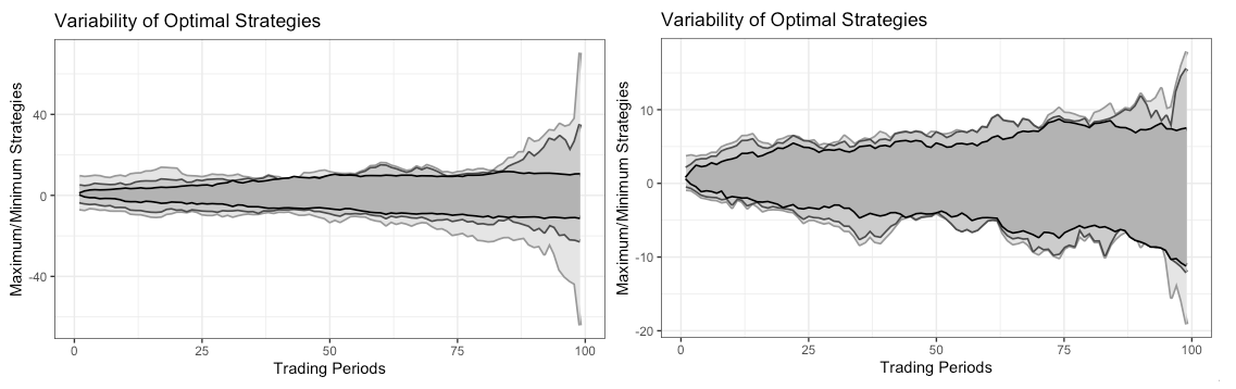
Figure 1: Black for the Natural trader, intermediate-gray for the Interval one and light-gray for the Precise one. We plot $\max_{k}\{\pi_{t}^{\mathbb{H}}(k)\}$ and $\max_{k}\{\pi_{t}^{\mathbb{H}}(k)\}$.

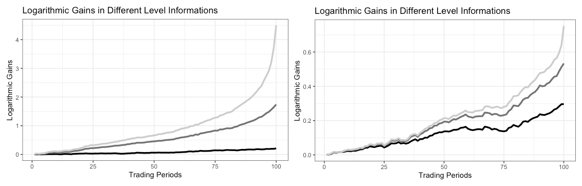
Figure 2: Black for the Natural trader, intermediate-gray for the Interval one and light-gray for the Precise one. We compared the average of the logarithmic gains for $\rho=0.75$ (left) and $\rho=0.25$ (right).

The simulations show that the logarithmic utility gains are greater if the Brownian motions $B^{S}$ and $B^{Y}$ are strongly correlated. If the correlation is negative, the agent can achieve the same gains because investing against the risky asset is allowed. It is shown also that if the investor possesses a more accurate information, she succeeds in gaining more by taking a more risky investment.

In Table 2 we fix $\rho=0.75$ and we study the interval information for the filtration $\mkern 1.5mu\overline{\mkern-1.5mu\mathbb{G}\mkern-1.5mu}\mkern 1.5mu$. We assume that this interval is always of the following form

$$(c_{1},c_{2})=((1-v)Y_{1},\ (1+v)Y_{1})\ ,\quad 0<v<1\ .$$

Whenever $v$ approaches 0, the Interval agent behaves more similar to the Precise one, as her information is more accurate, while as $v$ is near to 1, the she plays similar to the Natural one since her information is more imprecise. Again we omit the plot for $\rho=-0.75$.

		$\rho=0.75$
	$v=0.1$	$v=0.25$	$v=0.5$	$v=0.75$	$v=2$
$Gains$	4.65	3.55	2.47	2.03	3.14
$Q_{1}(\pi^{G})$	24.18	20.29	17.83	16.63	12.79
$Q_{2}(\pi^{G})$	26.27	25.24	24.51	20.63	16.41
$Q_{3}(\pi^{G})$	34.49	38.61	28.89	29.35	21.90
$Range(\pi^{G})$	139.72	107.97	70.33	65.98	41.54

Table 2: Results with different values of interval information.

7 Conclusions

In this paper, we showed how it is possible to include anticipative information about the stochastic interest rate process in a portfolio, and how to determine the modified optimal strategy. The model chosen for the interest rate is a general affine diffusion, a class that allows a complete analysis and contains in particular the Ornstein-Uhlenbeck process that is the one used in the Vasicek model. The model for the additional information is chosen in the class of linear type information. Under these assumptions the optimal portfolio is computed with the respect to different types of utilities, that is: logarithmic, CRRA and exponential. More detailed results and examples are then given for the logarithmic utility, where the model for the interest rate is given by the Ornstein-Uhlenbeck process and the privileged information is extended to the non-linear type. In particular it is computed the case of precise, half-bounded and bounded intervals by showing that in the first case the value of the information is infinite while in the other two cases it is finite. The possibility to obtain an infinite gain sounds surprising at a first sight, however it becomes clear when one considers the effect of the correlation coefficient that allows to transfer the information on the interest rate to the risky asset in proximity of the expiration date, due to the unbounded drift there. In particular, the $\mathbb{G}$-agent reveals to use some anticipative information as she accepts to take an unbounded risk near the expiration date supported by the knowledge she owns.

Appendix A Appendix

Lemma A.1.

$$\int_{-\infty}^{\infty}\left(\frac{1}{\bar{\Phi}(z)}+\frac{1}{\bar{\Phi}(-z)}\right)\left(\Phi^{\prime}(-z)\right)^{2}\Phi^{\prime}(a_{t}(z))dz<\infty$$

Proof.

Using the definition of $\widehat{I}$ in (5.8b) we have

$$\widehat{I}=\int_{-\infty}^{\infty}\left(\frac{1}{\bar{\Phi}(z)}+\frac{1}{\bar{\Phi}(-z)}\right)\Phi^{\prime}(-z)^{2}dz =\int_{-\infty}^{\infty}\frac{\Phi^{\prime}(-z)^{2}}{\bar{\Phi}(z)}dz+\int_{-\infty}^{\infty}\frac{\Phi^{\prime}(-z)^{2}}{\bar{\Phi}(-z)}dz$$

$$=2\left(\int_{-\infty}^{0}+\int_{0}^{\infty}\right)\frac{\Phi^{\prime}(z)}{\bar{\Phi}(z)}d\Phi(z)$$

We have

$$\int_{-\infty}^{0}\frac{\Phi^{\prime}(z)}{\bar{\Phi}(z)}d\Phi(z) \leq 2\int_{-\infty}^{0}\Phi^{\prime}(z)d\Phi(z)\leq\sqrt{\frac{2}{\pi}}\int_{-\infty}^{0}d\Phi(z)=\sqrt{\frac{2}{\pi}}\Phi(0)=\frac{1}{\sqrt{2\pi}}\ .$$

As for the other term, since $1/\bar{\Phi}(z)=e^{z^{2}/2}O(z)$ and $\Phi^{\prime}(z)=e^{-z^{2}/2}O(1)$ we have

$$\frac{\Phi^{\prime}(z)}{\bar{\Phi}(z)}=O(z)$$

and the result follows because $|z|$ is integrable with respect to $d\Phi(z)$. ∎

Lemma A.2.

$$\int_{0}^{T}\frac{\Psi_{T}^{2}(b_{2}\Psi^{-1})(t)^{2}}{\sqrt{\boldsymbol{V}[R_{t}|R_{0}]}\sqrt{\boldsymbol{V}[R_{T}|R_{t}]}}dt<\infty$$

Proof.

Having

$$\boldsymbol{V}[R_{t}|R_{0}] =\Psi_{t}^{2}\int_{0}^{t}(b_{2}\Psi^{-1})^{2}(x)dx$$

$$\boldsymbol{V}[R_{T}|R_{t}] =\Psi_{T}^{2}\int_{t}^{T}(b_{2}\Psi^{-1})^{2}(x)dx$$

it follows, by comparison criteria, that

$$1/\boldsymbol{V}[R_{t}|R_{0}] =O(1/\sqrt{t})$$

$$1/\boldsymbol{V}[R_{T}|R_{t}] =O(1/\sqrt{T-t})$$

and the result follows. ∎

Lemma A.3.

$$\int_{\mathbb{R}}\frac{\Psi_{t,T}\left[\Phi^{\prime}(z_{1})-\Phi^{\prime}(z_{2})\right]^{2}}{\sqrt{\boldsymbol{V}[R_{T}|R_{t}]}\left[\Phi\left(z_{2}\right)-\Phi\left(z_{1}\right)\right]\left[\Phi\left(-z_{2}\right)+\Phi\left(z_{1}\right)\right]}dx<\infty,$$

where we have defined $z_{1},\ z_{2}$ as,

$$z_{2}(x)=\frac{c_{2}-\boldsymbol{E}[R_{T},R_{t}=x]}{\sqrt{\boldsymbol{V}[R_{T}|R_{t}]}},\ \ z_{1}(x)=\frac{c_{1}-\boldsymbol{E}[R_{T},R_{t}=x]}{\sqrt{\boldsymbol{V}[R_{T}|R_{t}]}}$$

Proof.

We define function $h_{t}(x)=\Psi_{t,T}^{-1}\left(x-\Psi_{T}\int_{t}^{T}(a_{2}\Psi^{-1})(s)ds\right)$ monotonically increasing in x that holds $\boldsymbol{E}[R_{T}|R_{t}=h_{t}(x)]=x$ and let’s study the integral in separately intervals $\left(-\infty,h_{t}(c_{1})\right),\ \left(h_{t}(c_{1}),h_{t}(c_{2})\right)$$,\ \left(h_{t}(c_{2}),+\infty\right).$

In first case, we applied variable change in variable $z_{1}$ and obtain $z_{2}=z_{1}+\frac{c_{2}-c_{1}}{\sqrt{\boldsymbol{V}[R_{T}|R_{t}]}}$. We define $s_{t}=\frac{c_{2}-c_{1}}{\sqrt{\boldsymbol{V}[R_{T}|R_{t}]}}$ and its minimum in t as $s_{0}=\frac{c_{2}-c_{1}}{\sqrt{\boldsymbol{V}[R_{T}|R_{0}]}}>0$. And we get,

$$\int_{-\infty}^{h_{t}(c_{1})}I(x,t)dx =\int_{0}^{+\infty}\frac{\left[\Phi^{\prime}(z_{1})-\Phi^{\prime}(z_{1}+s_{t})\right]^{2}}{\left[\Phi\left(z_{1}+s_{t}\right)-\Phi\left(z_{1}\right)\right]\left[\Phi\left(-z_{1}-s_{t}\right)+\Phi\left(z_{1}\right)\right]}dz_{1}$$

$$=\int_{0}^{+\infty}\left(\frac{\left[\Phi^{\prime}(z_{1})-\Phi^{\prime}(z_{1}+s_{t})\right]^{2}}{\Phi\left(z_{1}+s_{t}\right)-\Phi\left(z_{1}\right)}+\frac{\left[\Phi^{\prime}(z_{1})-\Phi^{\prime}(z_{1}+s_{t})\right]^{2}}{\Phi\left(-z_{1}-s_{t}\right)+\Phi\left(z_{1}\right)}\right)dz_{1}$$

We are going to show that both terms are finite.

$$\int_{0}^{+\infty}\frac{\left[\Phi^{\prime}(z_{1})-\Phi^{\prime}(z_{1}+s_{t})\right]^{2}}{\Phi\left(z_{1}+s_{t}\right)-\Phi(z_{1})}dz_{1} \leq\int_{0}^{+\infty}\frac{\left[\Phi^{\prime}(z_{1})-\Phi^{\prime}(z_{1}+s_{t})\right]^{2}}{\Phi\left(z_{1}+\frac{c_{2}-c_{1}}{\sigma(T)}\right)-\Phi(z_{1})}dz_{1}$$

$$\leq\int_{0}^{+\infty}\frac{\left[\Phi^{\prime}(z_{1})\right]^{2}}{\Phi\left(z_{1}+\frac{c_{2}-c_{1}}{\sigma(T)}\right)-\Phi(z_{1})}dz_{1}$$

$$=\int_{0}^{1}\frac{\left[\Phi^{\prime}(z_{1})\right]^{2}}{\Phi\left(z_{1}+\frac{c_{2}-c_{1}}{\sigma(T)}\right)-\Phi(z_{1})}dz_{1}$$

$$+\int_{1}^{+\infty}\frac{\left[\Phi^{\prime}(z_{1})\right]^{2}}{\Phi\left(z_{1}+\frac{c_{2}-c_{1}}{\sigma(T)}\right)-\Phi(z_{1})}dz_{1}$$

The first integral is clearly bounded and for the second one, we apply comparison criteria with $f(z)=1/z^{2}$.

$$\lim_{z_{1}\to\infty}\frac{\sqrt{2\pi}z_{1}^{2}\left[\Phi^{\prime}(z_{1})\right]^{2}}{\Phi\left(z_{1}+\frac{c_{2}-c_{1}}{\sigma(T)}\right)-\Phi(z_{1})} =\lim_{z_{1}\to\infty}\frac{z_{1}^{2}\left[\exp\left(-{z_{1}^{2}}/{2}\right)\right]^{2}}{\int_{z_{1}}^{z_{1}+s_{0}}\exp(-u^{2}/2)du}$$

$$=\lim_{z_{1}\to\infty}\frac{2z_{1}\left[\exp\left(-{z_{1}^{2}}/{2}\right)\right]^{2}-2z_{1}^{3}\left[\exp\left(-{z_{1}^{2}}/{2}\right)\right]^{2}}{\exp(-(z_{1}+s_{0})^{2}/2)-\exp(-z_{1}^{2}/2)}$$

$$=\lim_{z_{1}\to\infty}\frac{2z_{1}\exp\left(-{z_{1}^{2}}/{2}\right)-2z_{1}^{3}\exp\left(-{z_{1}^{2}}/{2}\right)}{\exp(-z_{1}s_{0})\exp(-s_{0}^{2}/2)-1}\to 0,$$

where, in the second equality, we have used L’Hopital Rule and we conclude the integral is finite in $(1,+\infty)$. With the other term we have the following bound,

$$\int_{0}^{+\infty}\frac{\left[\Phi^{\prime}(z_{1})-\Phi^{\prime}(z_{1}+s_{t})\right]^{2}}{\Phi(-z_{1}-s_{t})+\Phi(z_{1})}dz_{1} \leq\int_{0}^{+\infty}\frac{\left[\Phi^{\prime}(z_{1})-\Phi^{\prime}(z_{1}+s_{t})\right]^{2}}{\Phi(z_{1})}dz_{1}$$

$$\leq 2\int_{0}^{+\infty}\left[\Phi^{\prime}(z_{1})-\Phi^{\prime}(z_{1}+s_{t})\right]^{2}dz_{1}$$

$$\leq 2\int_{0}^{+\infty}\left[\Phi^{\prime}(z_{1})\right]^{2}dz_{1}=\frac{1}{\sqrt[]{2}}$$

We analyze now interval $(h_{t}(c_{2}),+\infty)$ and we proceed in the same way, but doing change variable in $z_{2}=\frac{c_{2}-\mu(T-t,x)}{\sigma(T-t)}$ and we get,

$$\int^{+\infty}_{h_{t}(c_{2})}I(x,t)dx =\int_{-\infty}^{0}\frac{\left[\Phi^{\prime}(z_{2}-s_{t})-\Phi^{\prime}(z_{2})\right]^{2}}{\left[\Phi\left(z_{2}\right)-\Phi\left(z_{2}-s_{t}\right)\right]\left[\Phi\left(-z_{2}\right)+\Phi\left(z_{2}-s_{t}\right)\right]}dz_{2}$$

$$=\int_{-\infty}^{0}\left(\frac{\left[\Phi^{\prime}(z_{2}-s_{t})-\Phi^{\prime}(z_{2})\right]^{2}}{\left[\Phi\left(z_{2}\right)-\Phi\left(z_{2}-s_{t}\right)\right]}+\frac{\left[\Phi^{\prime}(z_{2}-s_{t})-\Phi^{\prime}(z_{2})\right]^{2}}{\left[\Phi\left(-z_{2}\right)+\Phi\left(z_{2}-s_{t}\right)\right]}\right)dz_{2}$$

We are going to show that both terms are finite.

$$\int_{-\infty}^{0}\frac{\left[\Phi^{\prime}(z_{2}-s_{t})-\Phi^{\prime}(z_{2})\right]^{2}}{\left[\Phi\left(z_{2}\right)-\Phi\left(z_{2}-s_{t}\right)\right]}dz_{2} \leq\int_{-\infty}^{0}\frac{\left[\Phi^{\prime}(z_{2}-s_{t})-\Phi^{\prime}(z_{2})\right]^{2}}{\left[\Phi\left(z_{2}\right)-\Phi\left(z_{2}-s_{0}\right)\right]}dz_{2}$$

$$\leq\int_{-\infty}^{0}\frac{\left[\Phi^{\prime}(z_{2})\right]^{2}}{\left[\Phi\left(z_{2}\right)-\Phi\left(z_{2}-s_{0}\right)\right]}dz_{2}$$

And applying the same reasoning as before, we conclude that integral is finite. Finally,

$$\int_{-\infty}^{0}\frac{\left[\Phi^{\prime}(z_{2}-s_{t})-\Phi^{\prime}(z_{2})\right]^{2}}{\left[\Phi\left(-z_{2}\right)+\Phi\left(z_{2}-s_{t}\right)\right]}dz_{2} \leq\int_{-\infty}^{0}\frac{\left[\Phi^{\prime}(z_{2}-s_{t})-\Phi^{\prime}(z_{2})\right]^{2}}{\Phi\left(-z_{2}\right)}dz_{2}$$

$$\leq 2\int_{-\infty}^{0}\left[\Phi^{\prime}(z_{2})\right]^{2}dz_{2}=\frac{1}{\sqrt[]{2}}$$

We analyze now the last interval $\mathcal{I}=(h_{t}(c_{1}),h_{t}(c_{2}))$. We could proceed doing variable change, for example, in $z_{2}$. The point $c_{1}$ is transformed to

$$z_{2}(c_{1})=\frac{c_{2}-\boldsymbol{E}[R_{T}|R_{t}=c_{1}]}{\sqrt{\boldsymbol{V}[R_{T}|R_{t}]}}=\frac{c_{2}-c_{1}}{\sqrt{\boldsymbol{V}[R_{T}|R_{t}]}}+\frac{c_{1}-\boldsymbol{E}[R_{T}|R_{t}=c_{1}]}{\sqrt{\boldsymbol{V}[R_{T}|R_{t}]}}=:s_{t}+r_{t}\ .$$

Then we get,

$$\int_{h_{t}(c_{1})}^{h_{t}(c_{2})}I(x,t)dx =\int_{0}^{s_{t}+r_{t}}\frac{(\Phi^{\prime}(z_{2})-\Phi^{\prime}(z_{2}-s_{t}))^{2}}{\Phi(z_{2})-\Phi(z_{2}-s_{t})}+\frac{(\Phi^{\prime}(z_{2})-\Phi^{\prime}(z_{2}-s_{t}))^{2}}{\Phi(-z_{2})+\Phi(z_{2}-s_{t})}dz_{2}$$

Now, we are going to show that both integrals are bounded and we separate $[0,s_{t}]$ and $[s_{t},s_{t}+r_{t}]$.

$$\int_{0}^{s_{t}}\frac{(\Phi^{\prime}(z_{2})-\Phi^{\prime}(z_{2}-s_{t}))^{2}}{\Phi(z_{2})-\Phi(z_{2}-s_{t})}dz_{2} =2\int_{0}^{s_{t}/2}\frac{(\Phi^{\prime}(z_{2})-\Phi^{\prime}(z_{2}-s_{t}))^{2}}{\Phi(z_{2})-\Phi(z_{2}-s_{t})}dz_{2}$$

$$\leq 2\int_{0}^{s_{t}/2}\frac{\Phi^{\prime}(z_{2})^{2}}{\Phi(z_{2})-\Phi(z_{2}-s_{0})}dz_{2}$$

$$\leq 2\int_{0}^{\infty}\frac{\Phi^{\prime}(z_{2})^{2}}{\Phi(z_{2})-\Phi(z_{2}-s_{0})}dz_{2}$$

Which is finite, trivially in $[0,1]$ and using criteria comparison with $f(z)=z^{-2}$ in $[1,+\infty]$. Now we show that,

$$\int_{s_{t}}^{s_{t}+r_{t}}\frac{(\Phi^{\prime}(z_{2})-\Phi^{\prime}(z_{2}-s_{t}))^{2}}{\Phi(z_{2})-\Phi(z_{2}-s_{t})}dz_{2} =\int_{0}^{r_{t}}\frac{(\Phi^{\prime}(z_{1}+s_{t})-\Phi^{\prime}(z_{1}))^{2}}{\Phi(z_{1}+s_{t})-\Phi(z_{1})}dz_{1}$$

$$\leq\int_{0}^{r_{t}}\frac{\Phi^{\prime}(z_{1})^{2}}{\Phi(z_{1}+s_{0})-\Phi(z_{1})}dz_{1}<+\infty.$$

Now, we analyze the other term in the integral,

$$\int_{0}^{s_{t}+r_{t}}\frac{(\Phi^{\prime}(z_{2})-\Phi^{\prime}(z_{2}-s_{t}))^{2}}{\Phi(-z_{2})+\Phi(z_{2}-s_{t})}dz_{2} =\int_{0}^{s_{t}}\frac{(\Phi^{\prime}(z_{2})-\Phi^{\prime}(z_{2}-s_{t}))^{2}}{\Phi(-z_{2})+\Phi(z_{2}-s_{t})}dz_{2}$$

$$+\int_{s_{t}}^{s_{t}+r_{t}}\frac{(\Phi^{\prime}(z_{2})-\Phi^{\prime}(z_{2}-s_{t}))^{2}}{\Phi(-z_{2})+\Phi(z_{2}-s_{t})}dz_{2}$$

$$=2\int_{0}^{s_{t}/2}\frac{(\Phi^{\prime}(z_{2})-\Phi^{\prime}(z_{2}-s_{t}))^{2}}{\Phi(-z_{2})+\Phi(z_{2}-s_{t})}dz_{2}$$

$$+\int_{s_{t}}^{s_{t}+r_{t}}\frac{(\Phi^{\prime}(z_{2})-\Phi^{\prime}(z_{2}-s_{t}))^{2}}{\Phi(-z_{2})+\Phi(z_{2}-s_{t})}dz_{2}$$

The second integral is trivially bound and the last equality holds because the function we are integrating is symmetric with respect $s_{t}/2$.

$$\Phi^{\prime}(z_{2})-\Phi^{\prime}(z_{2}-s_{t}) =\frac{1}{\sqrt[]{2\pi}}\left[\exp\left(-\frac{z_{2}^{2}}{2}\right)-\exp\left(-\frac{(z_{2}-s_{t})^{2}}{2}\right)\right]$$

$$=\frac{1}{\sqrt[]{2\pi}}\exp\left(-\frac{z_{2}^{2}}{2}\right)\left[1-\exp\left(-\frac{s_{t}^{2}-2z_{2}s_{t}}{2}\right)\right]$$

$$\leq\frac{1}{\sqrt[]{2\pi}}\exp\left(-\frac{z_{2}^{2}}{2}\right)$$

As $0\leq z_{2}\leq s_{t}/2$, we have $s_{t}^{2}-2z_{2}s_{t}\geq 0$ and we could apply the last inequality.

$$\int_{c_{1}}^{c_{2}}I(x,t)dx \leq\sqrt[]{\frac{2}{\pi}}\int_{0}^{s_{t}/2}\frac{\exp\left(-z_{2}^{2}\right)}{\Phi(-z_{2})+\Phi(z_{2}-s_{t})}dz_{2}\leq\int_{0}^{s_{t}/2}\frac{\exp\left(-z_{2}^{2}\right)}{\Phi(-z_{2})}dz_{2}$$

$$\leq\int_{0}^{+\infty}\frac{\exp\left(-z_{2}^{2}\right)}{\Phi(-z_{2})}dz_{2}=\int_{0}^{1}\frac{\exp\left(-z_{2}^{2}\right)}{\Phi(-z_{2})}dz_{2}+\int_{1}^{+\infty}\frac{\exp\left(-z_{2}^{2}\right)}{\Phi(-z_{2})}dz_{2}$$

The first integral is trivially bounded. We apply comparison criteria with $f(z)=1/z^{2}$ to proof that the second one is finite too.

∎

References

- [1] Igor Pikovsky and Ioannis Karatzas “Anticipative Portfolio Optimization” In Advances in Applied Probability 28.4, 1996, pp. 1095–1122
- [2] Jürgen Amendinger, Peter Imkeller and Martin Schweizer “Additional logarithmic utility of an insider” In Stochastic Processes and their Applications 75.2, 1998, pp. 263–286 DOI: 10.1016/S0304-4149(98)00014-3
- [3] Jürgen Amendinger, Dirk Becherer and Martin Schweizer “A monetary value for initial information in portfolio optimization” In Finance and Stochastics 7.1, 2003, pp. 29–46 DOI: 10.1007/s007800200075
- [4] Peter Imkeller, Monique Pontier and Ferenc Weisz “Free lunch and arbitrage possibilities in a financial market model with an insider” In Stochastic Processes and their Applications 92.1, 2001, pp. 103–130 DOI: https://doi.org/10.1016/S0304-4149(00)00071-5
- [5] Stefan Ankirchner and Peter Imkeller “Finite utility on financial markets with asymmetric information and structure properties of the price dynamics” In Annales de l’Institut Henri Poincaré, Statistics 41.3, 2005, pp. 479–503 DOI: 10.1016/j.anihpb.2004.03.008
- [6] Huy N Chau, Andrea Cosso and Claudio Fontana “The value of informational arbitrage” In Finance and Stochastic 24, 2020, pp. 277–307 DOI: 10.1007/s00780-020-00418-3
- [7] Philip A. Ernst and L… Rogers “The Value of Insight” In Mathematics of Operations Research 45.4, 2020, pp. 1193–1209 DOI: 10.1287/moor.2019.1028
- [8] Anna Aksamit and Monique Jeanblanc “Enlargement of Filtration with Finance in View” Springer International Publishing, 2017 DOI: 10.1007/978-3-319-41255-9
- [9] Younes Kchia and Philip Protter “Progressive filtration expansions via a process, with applications to insider trading” In International Journal of Theoretical and Applied Finance 18.04, 2015, pp. 1550027 DOI: 10.1142/S0219024915500272
- [10] Markus Hess “An anticipative stochastic minimum principle under enlarged filtrations” In Stochastic Analysis and Applications 39.2 Taylor & Francis, 2021, pp. 252–277 DOI: 10.1080/07362994.2020.1794894
- [11] Oldrich Vasicek “An equilibrium characterization of the term structure” In Journal of Financial Economics 5.2, 1977, pp. 177–188 DOI: 10.1016/0304-405X(77)90016-2
- [12] Yutian Nie and Vadim Linetsky “Sticky reflecting Ornstein-Uhlenbeck diffusions and the Vasicek interest rate model with the sticky zero lower bound” In Stochastic Models 36.1 Taylor & Francis, 2020, pp. 1–19 DOI: 10.1080/15326349.2019.1630287
- [13] Bogdan Iftimie, Monique Jeanblanc and Thomas Lim “Optimization problem under change of regime of interest rate” In Stochastics and Dynamics 16.05, 2016, pp. 1650015 DOI: 10.1142/S0219493716500155
- [14] Ralf Korn and Holger Kraft “A Stochastic Control Approach to Portfolio Problems with Stochastic Interest Rates” In SIAM J. Control and Optimization 40, 2001, pp. 1250–1269
- [15] Jean Jacod “Grossissement initial, hypothése (H’) et théoréme de Girsanov” In Grossissements de filtrations: exemples et applications Springer, 1985, pp. 15–35
- [16] Bernardo D’Auria and Jose-Antonio Salmeron “Insider information and its relation with the arbitrage condition and the utility maximization problem” In Mathematical Biosciences and Engineering 17.2, 2020, pp. 998–1019 DOI: 10.3934/mbe.2020053
- [17] Freddy Delbaen and Walter Schachermayer “The Mathematics of Arbitrage”, Springer Finance Springer-Verlag, 2006
- [18] Monique Jeanblanc, Marc Yor and Marc Chesney “Mathematical Methods for Financial Markets”, Springer Finance Springer London, 2009
- [19] Claudio Fontana “The strong predictable representation property in initially enlarged filtrations under the density hypothesis” In Stochastic Processes and their Applications 128.3, 2018, pp. 1007–1033 DOI: https://doi.org/10.1016/j.spa.2017.06.015
- [20] Ioannis Karatzas, John P. Lehoczky, Steven E. Shreve and Gan-Lin Xu “Martingale and Duality Methods for Utility Maximization in an Incomplete Market” In SIAM Journal on Control and Optimization 29.3, 1991, pp. 702–730 DOI: 10.1137/0329039
- [21] Claudio Fontana “A note on arbitrage, approximate arbitrage and the fundamental theorem of asset pricing” In Stochastics 86.6 Taylor & Francis, 2014, pp. 922–931 DOI: 10.1080/17442508.2014.895358
- [22] Damir Filipovic “Term-Structure Models” Springer Finance, 2009 DOI: 10.1007/978-3-540-68015-4
- [23] Huyên Pham and Marie-Claire Quenez “Optimal Portfolio in Partially Observed Stochastic Volatility Models” In The Annals of Applied Probability 11.1 Institute of Mathematical Statistics, 2001, pp. 210–238 DOI: 10.1214/aoap/998926991
- [24] Peter Imkeller “Malliavin’s Calculus in Insider Models: Additional Utility and Free Lunches” In Mathematical Finance 13.1, 2003, pp. 153–169 DOI: 10.1111/1467-9965.00011
- [25] Giulia Di Nunno, Bernt Øksendal and Frank Proske “Malliavin Calculus for Levy Processes with Applications to Finance”, Universitext Springer, 2009
- [26] Andreas Basse-O’Connor “Representation of Gaussian semimartingales with applications to the covariance function” In Stochastics 82.4 Taylor & Francis, 2010, pp. 381–401 DOI: 10.1080/17442500903251857
- [27] Bernt Øksendal and Elin Engen Røse “A White Noise Approach to Insider Trading” In Let Us Use White Noise World Scientific, 2017, pp. 191–203 DOI: 10.1142/9789813220942“˙0006
- [28] Joseph Diestel and Jerry Jerry Uhl “Vector measures” With a foreword by B. J. Pettis, Mathematical Surveys, No. 15 Providence, R.I.: American Mathematical Society, 1977, pp. xiii+322
- [29] Y. Kakihara “Radon-Nikodým Derivatives of Hilbert Space Valued Measures” In Journal of Statistical Theory and Practice 5.3 Taylor & Francis, 2011, pp. 453–473 DOI: 10.1080/15598608.2011.10412040
- [30] B. Acciaio, C. Fontana and C. Kardaras “Arbitrage of the first kind and filtration enlargements in semimartingale financial models” In Stochastic Processes and their Applications 126.6, 2016, pp. 1761–1784 DOI: 10.1016/j.spa.2015.12.004