Interpretable Vector AutoRegressions with Exogenous Time Series

Abstract

The Vector AutoRegressive (VAR) model is fundamental to the study of multivariate time series. Although VAR models are intensively investigated by many researchers, practitioners often show more interest in analyzing VARX models that incorporate the impact of unmodeled exogenous variables (X) into the VAR. However, since the parameter space grows quadratically with the number of time series, estimation quickly becomes challenging. While several proposals have been made to sparsely estimate large VAR models, the estimation of large VARX models is under-explored. Moreover, typically these sparse proposals involve a lasso-type penalty and do not incorporate lag selection into the estimation procedure. As a consequence, the resulting models may be difficult to interpret. In this paper, we propose a lag-based hierarchically sparse estimator, called "HVARX", for large VARX models. We illustrate the usefulness of HVARX on a cross-category management marketing application. Our results show how it provides a highly interpretable model, and improves out-of-sample forecast accuracy compared to a lasso-type approach.

1 Introduction

Autocorrelated multivariate time series are primarily modeled using Vector AutoRegressive (VAR) models. Applications are found in diverse fields such as machine learning (e.g., Melnyk and Banerjee, 2016), macro-economics (e.g., Banbura et al., 2010), and marketing (e.g., Gelper et al., 2016). In a VAR${}_{k}(p)$ model, a stationary $k$-dimensional vector time series $\{{y}_{t}\}$ is modeled in terms of its previous $p$ values. In low-dimensional settings, in which $k^{2}p$ is small relative to the series length $T$, VAR models can be estimated using multivariate least squares. However, this approach becomes imprecise or even intractable in large VAR models, in which $k^{2}p$ can exceed $T$. Recent interest in modeling high dimensional time series has driven many advances in penalized estimators for large VARs (e.g., Davis et al., 2016, Basu and Michailidis, 2015, Gelper et al., 2016, Nicholson et al., 2016). Most utilize an $\ell_{1}$-penalty (lasso-penalty, Tibshirani, 1996) to obtain sparse parameter estimates.

While VAR models are more intensively investigated, practitioners are often more interested in estimating "VARX" models, i.e., vector autoregressions with additional unmodeled exogenous (X) time series components. In economics, for example, VARX models have become popular to model small open economies given U.S. variables. The VARX is also of interest in scenarios where one desires forecasts from only a subset of a larger set of time series. In marketing, for instance, one may use the VARX to predict sales of several related products using their past sales, price and promotion information.

However, large VARX models - which are as heavily overparameterized as large VARs - have received only limited attention in the literature (see, e.g., Nicholson et al. 2017). Moreover, endogenous and exogenous components have different lag orders, and lag selection by classical information criteria is intractable, in general. While $\ell_{1}$-type estimators can resolve the dimensionality issue, they are not well suited to solve lag selection issues. The resulting models are not easily interpretable and Nicholson et al. (2016) show that the prediction performance of these estimators substantially deteriorates for VARs with large lag orders as they select many high lag order coefficients.

To simultaneously address the dimensionality and lag selection issues while providing highly interpretable estimates, we propose a lag-based hierarchically sparse estimation procedure, "HVARX", for large VARX. Like most papers on large VAR estimation, our parameter estimates are sparse to accommodate the dimensionality issue. Unlike other approaches, we embed automatic lag selection of both the exogenous and endogenous components into estimation. We build on the HVAR penalties of Nicholson et al. (2016), which use hierarchical group lasso penalties (e.g., Yuan and Lin, 2006 for group lasso) in place of $\ell_{1}$-penalties. The proposed estimation procedure is very flexible: a separate lag order is learned for each endogenous and exogenous series in each marginal equation of the VARX. The result is a parsimonious, highly interpretable model with low lag orders. We apply HVARX to estimate cross-category demand effects among a large number of product categories for a particular U.S. grocery store. Our results show that HVARX provides highly interpretable results, and considerably improves forecast accuracy compared to a lasso-type estimator.

2 Methodology

Model.

In a VARX${}_{k,m}(p,s)$, a stationary $k$-dimensional vector series $\{{y}_{t}\}$ is modeled in terms of its own past $p$ values and the past $s$ values of a stationary $m$-dimensional vector series $\{{x}_{t}\}$:

$${y}_{t}=\sum_{\ell=1}^{p}\Phi_{\ell}{y}_{t-\ell}+\sum_{j=1}^{s}B_{j}{x}_{t-j}+{\epsilon}_{t},$$ (1)

where $\{\Phi_{\ell}\in\mathbb{R}^{k\times k}\}_{\ell=1}^{p}$ are endogenous coefficient matrices, $\{B_{j}\in\mathbb{R}^{k\times m}\}_{j=1}^{s}$ are exogenous coefficient matrices, and $\{{\epsilon}_{t}\}$ is a $k$-dimensional mean-zero white noise vector time series. We assume, without loss of generality, that all time series are mean-centered and thus omit an intercept. A VAR${}_{k}(p)$ model is a special case of the VARX${}_{k,m}(p,s)$ model in (1) where $m=0$. In the remainder, we consider the VARX${}_{k,m}(p,s)$ in compact matrix notation: ${Y}={\Phi}{Z}+{B}{X}+{{E}},$ where ${Y}=[{y}_{\bar{o}+1}\ldots{y}_{T}]\in\mathbb{R}^{k\times({T-\bar{o}})},$ ${Z}=[{z}_{\bar{o}+1}\ldots{z}_{T}]\in\mathbb{R}^{kp\times({T-\bar{o}})}$, with ${z}_{t}=[{y}^{\top}_{t-1}\ldots{y}^{\top}_{t-{p}}]^{\top}\in\mathbb{R}^{(kp\times 1)},$ ${X}=[{x}_{\bar{o}+1}\ldots{x}_{T}]\in\mathbb{R}^{ms\times({T-\bar{o}})}$ with ${x}_{t}=[x^{\top}_{t-1}\ldots x^{\top}_{t-s}]^{\top}\in\mathbb{R}^{(ms\times 1)}$, with $\bar{o}=\max(p,s)$, ${{E}}=[{\epsilon}_{\bar{o}+1}\ldots{\epsilon}_{T}]\in\mathbb{R}^{k\times({T-\bar{o}})},{\Phi}=[{\Phi}_{1}\ldots{\Phi}_{p}]\in\mathbb{R}^{k\times kp},$ and ${B}=[{B}_{1}\ldots{B}_{s}]\in\mathbb{R}^{k\times ms}.$

Estimator.

To obtain estimates $(\widehat{\Phi},\widehat{B})$, we use a sparsity inducing estimator which places a lag-based hierarchical group lasso (HLag; Nicholson et al. 2016) penalty on both the endogenous and exogenous parameters. The parameter estimates are obtained as

$$\!(\widehat{{\Phi}},\widehat{{B}})\!=\!\underset{{\Phi},{B}}{\operatorname{argmin}}\!\left\{\!\dfrac{1}{2}\|{Y}-{\Phi}{Z}-{B}{X}\|_{F}^{2}\!+\!\lambda_{{\Phi}}\sum_{i=1}^{k}\sum_{d=1}^{k}\sum_{\ell=1}^{p}\|{\Phi}_{(\ell:p),id}\|_{2}\!+\!\lambda_{{B}}\sum_{i=1}^{k}\sum_{r=1}^{m}\sum_{j=1}^{s}\|{B}_{(j:s),ir}\|_{2}\!\right\}\!,\!\!$$ (2)

where $\|\cdot\|_{F}$ denotes the Frobenius norm, ${\Phi}_{(\ell:p),id}=\left[{\Phi}_{\ell,id}\ldots{\Phi}_{p,id}\right]\in\mathbb{R}^{(p-\ell+1)}$, and ${B}_{(j:s),ir}=\left[{B}_{j,ir}\ldots{B}_{s,ir}\right]\in\mathbb{R}^{(s-j+1)}$. This defines the HVARX estimator. Figure 1 illustrates how the nested group principle can be used to achieve hierarchical sparsity. By using this hierarchical group structure, the estimator forces lower lagged coefficients of a particular time series to be selected before its higher order time lagged coefficients. As such, it automatically determines the maximum lag order for the corresponding component (for more, see Nicholson et al. 2016). HVARX is highly flexible as each (endogenous and exogenous) series has its own lag structure in each marginal equation of the VARX.

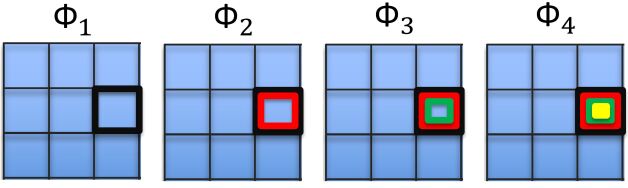
Figure 1: Lag-based hierarchical group structure of element (2,3) of the $\Phi$ matrices for an illustrative VARX model with $k=3$ and $p=4$. The first group (black) contains element (2,3) of all $\Phi$ matrices. The second group (red) is nested in the first and only contains element (2,3) of ($\Phi_{2},\Phi_{3},\Phi_{4}$). The nested structure continues with the green and yellow groups.

The penalty parameters $\lambda_{{\Pi}}>0$ and $\lambda_{{B}}>0$ regulate the degree of sparsity in $\widehat{{\Phi}}$ and $\widehat{{B}}$, respectively, and are selected using a time-series cross-validation approach (see Wilms et al. 2017b). To compute HVARX, we use the Proximal Gradient Algorithm in Wilms et al. (2017b, Algorithm 2). An implementation of our method is available in the R package bigtime (Wilms et al., 2017a).

Theoretical Properties.

Assuming the VARX process $\{y_{t}\}$ is stable with Gaussian innovations $\{\epsilon_{t}\}$, theoretical analysis of HVARX and "$\ell_{1}$-VARX", the standard lasso estimator of the VARX model, can be conducted under a suitable Restricted Eigenvalue (RE) assumption on the design matrix $\tilde{Z}=[Z^{\top},X^{\top}]$ and a deviation bound on $\tilde{Z}^{\top}E$ (cf. Basu and Michailidis, 2015 for more details). The stability properties of a Gaussian VARX model have been studied recently in Lin and Michailidis (2017), along with the validity of necessary RE and deviation conditions for the $\ell_{1}$-VARX when the matrix $\Phi$ is sparse and the matrix $B$ is low-rank. A straightforward adaptation of these results, coupled with the deviation bounds in Proposition 2.4 of Basu and Michailidis (2015) shows that $\ell_{1}$-VARX can consistently estimate $\Phi$ and $B$ in a high-dimensional regime where the time series dimensions $k$ and $m$ grow exponentially with sample size $(T-\bar{o})$. Theoretical properties of HVARX in high-dimension can be explored along the same route as $\ell_{1}$-VARX, although additional challenges remain due to the non-separable nature of the HLag penalty. We expect to leverage recent advances in the theory of overlapping group Lasso to address these challenges.

3 Marketing Application

Retailers carry products in a large variety of categories such as soft drinks. Successful cross-category management requires retailers to understand "cross-category demand effects", i.e., the effects of prices, promotions, and sales of one category on the sales (or demand) of another product category. The VARX model can be used to estimate these demand effects, with the sales series taken as the endogenous time series and the price and promotion series taken as the exogenous time series.

Data.

We use data on 16 product categories from a grocery store of Dominick’s, a U.S. supermarket chain. Sales, price, and promotion data are collected from January 1993 to July 1994, hence $T=76$, and are publicly available from https://research.chicagobooth.edu/kilts/marketing-databases/dominicks. For more information on the calculation of the sales, price, and promotion variables, see Srinivasan et al. (2004). We apply the HVARX model with $k=16$ endogenous sales series and $m=32$ exogenous price and promotion series, with $p=s=\lfloor 1.5\sqrt{T}\rfloor=13$.

Estimated Demand Effects.

Since HVARX performs automatic lag selection, it returns the effective maximum lag orders of each elementwise component. Consider the $k\times k$ endogenous lag matrix $\widehat{L}_{\widehat{\Phi}}$ and $k\times m$ exogenous lag matrix $\widehat{L}_{\widehat{B}}$ of an estimated VARX with elements

$$\widehat{L}_{\widehat{\Phi},id}=\max\{\ell:\widehat{\Phi}_{\ell,id}\neq 0\},\ \ \ \text{and}\ \ \ \widehat{L}_{\widehat{B},ir}=\max\{s:\widehat{B}_{s,ir}\neq 0\},$$

and $\widehat{L}_{\widehat{\Phi},id}=0$ if $\widehat{\Phi}_{\ell,id}=0$ for all $\ell=1,\ldots,p$; analogously for $\widehat{L}_{\widehat{B}}$. The lag matrix $\widehat{L}_{\widehat{\Phi}}$ gives the maximal lag for each endogenous series $d$ in each marginal equation $i$ for an estimated VARX. Similarly, $\widehat{L}_{\widehat{B}}$ gives the maximal lag for each exogenous series $r$ in each equation $i$.

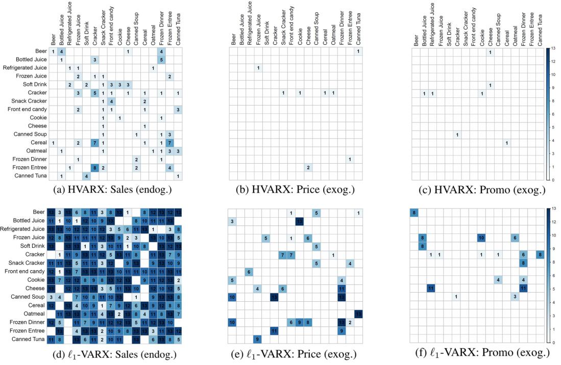
Figure 2: Panel (a) and (d): Lag matrix of endogenous sales time series, panel (b) and (e): exogenous price time series and panel (c) and (f): exogenous promotion time series, for the HVARX (top) and the $\ell_{1}$-VARX (bottom) estimators, respectively. The maximum orders in the VARX were $\lfloor 1.5\sqrt{T}\rfloor=13$.

Figure 2 compares the estimated lag matrices of HVARX (top) to those of $\ell_{1}$-VARX (bottom). The first column gives the lag matrices of the endogenous sales time series (i.e., $\widehat{L}_{\widehat{\Phi}}$), the second column gives the lag matrices of the exogenous price time series, and the third column gives the lag matrices of the exogenous promotion time series. Note that panels (b)-(c); (e)-(f) combined give the $16\times 32$-matrix $\widehat{L}_{\widehat{B}}$. The lag matrices of HVARX are overall sparser than those of $\ell_{1}$-VARX, with considerably lower maximal lag orders for the endogenous sales time series. The Bayesian Information Criterion confirms the model estimated by HVARX to provide a better in-sample fit than the model estimated by $\ell_{1}$-VARX: BIC=11.08 versus BIC=43.11, respectively.

By encouraging the maximal lag orders to be small, HVARX gives a highly interpretable model. The lag matrix of the endogenous time series (panel a) shows the prevalence of within-category sales effects: each sales product category (except cheese) is influenced by its own past sales values (i.e., non-zero diagonal elements). Only a minority of cross-category sales effects are estimated as non-zero (i.e., non-zero off-diagonal elements). The lag matrices of exogenous time series (panel b and c) are very sparse: for HVARX, 8 out of 256 entries of the price lag matrix and 7 out of 256 entries of the promotion lag matrix are non-zero. These lag matrices mainly reveal cross-category effects possibly due to substitution or affinity in consumption. The more parsimonious model obtained with HVARX also gives more accurate forecasts, as discussed in the following paragraph.

Forecast Accuracy.

We compare the forecast accuracy of HVARX and $\ell_{1}$-VARX. To assess forecast accuracy, we use an expanding window forecast approach (see Wilms et al., 2017b) where we compute one-step-ahead forecasts for the last 15% of the observations. The overall forecast performance is then measured by the Mean Squared Forecast Error (averaged over all time series and all time points). HVARX attains a lower MSFE than $\ell_{1}$-VARX: MSFE=0.391 versus MSFE=0.453. A Diebold-Martiano (Diebold and Mariano, 1995) test also confirms this improvement in forecast accuracy to be significant at the 5% significance level.

Acknowledgments

IW was supported by the Research Foundation-Flanders (FWO-12M8217N), JB was supported by an NSF CAREER award (DMS-1748166), DSM was supported by an NSF CAREER award (DMS-1455172), a Xerox PARC Faculty Research Award, and Cornell University Atkinson Center for a Sustainable Future (AVF-2017).

References

- Banbura et al. (2010) Banbura, M.; Giannone, D. and Reichlin, L. (2010), “Large Bayesian vector auto regressions,” Journal of Applied Econometrics, 25(1), 71–92.
- Basu and Michailidis (2015) Basu, S. and Michailidis, G. (2015), “Regularized estimation in sparse high-dimensional time series models,” The Annals of Statistics, 43(4), 1535–1567.
- Davis et al. (2016) Davis, R.; Zang, P. and Zheng, T. (2016), “Sparse vector autoregressive modeling,” Journal of Computational and Graphical Statistics, 25(4), 1077–1096.
- Diebold and Mariano (1995) Diebold, F. and Mariano, R. (1995), “Comparing predictive accuracy,” Journal of Business and Economic Statistics, 13, 253–263.
- Gelper et al. (2016) Gelper, S.; Wilms, I. and Croux, C. (2016), “Identifying demand effects in a large network of product categories,” Journal of Retailing, 92(1), 25–39.
- Lin and Michailidis (2017) Lin, J. and Michailidis, G. (2017), “Regularized estimation and testing for high-dimensional multi-block vector-autoregressive models,” arXiv preprint arXiv:1708.05879.
- Melnyk and Banerjee (2016) Melnyk, I. and Banerjee, A. (2016), “Estimating structured vector autoregressive models,” Proceedings of the 33rd International Conference on Machine Learning, New York, NY, USA, 2016, JMLR: W&CP volume48.
- Nicholson et al. (2017) Nicholson, W.; Matteson, D. S. and Bien, J. (2017), “VARX-L: Structured regularization for large vector autoregressions with exogenous variables,” International Journal of Forecasting, 33(3), 627–651.
- Nicholson et al. (2016) Nicholson, W. B.; Bien, J. and Matteson, D. S. (2016), “High dimensional forecasting via interpretable vector autoregression,” arXiv, 1412.5250v2.
- Srinivasan et al. (2004) Srinivasan, S.; Pauwels, K.; Hanssens, D. and Dekimpe, M. (2004), “Do promotions benefit manufacturers, retailers, or both?” Management Science, 50(5), 617–629.
- Tibshirani (1996) Tibshirani, R. (1996), “Regression shrinkage and selection via the lasso,” Journal of the Royal Statistical Society Series B, 58(1), 267–288.
- Wilms et al. (2017a) Wilms, I.; Basu, S.; Bien, J. and Matteson, D. S. (2017a), bigtime: Sparse Estimation of Large Time Series Models, R package version 0.1.0. https://CRAN.R-project.org/package=bigtime.
- Wilms et al. (2017b) — (2017b), “Sparse identification and estimation of high-dimensional vector autoregressive moving averages,” arXiv:1707.09208.
- Yuan and Lin (2006) Yuan, M. and Lin, Y. (2006), “Model selection and estimation in regression with grouped variables,” Journal of the Royal Statistical Society Series B, 68, 49–67.