Majorana quasiparticles in semiconducting carbon nanotubes

Abstract

Engineering effective p-wave superconductors hosting Majorana quasiparticles (MQPs) is nowadays of particular interest, also in view of the possible utilization of MQPs in fault-tolerant topological quantum computation. In quasi one-dimensional systems, the parameter space for topological superconductivity is significantly reduced by the coupling between transverse modes. Together with the requirement of achieving the topological phase under experimentally feasible conditions, this strongly restricts in practice the choice of systems which can host MQPs. Here we demonstrate that semiconducting carbon nanotubes (CNTs) in proximity with ultrathin s-wave superconductors, e.g. exfoliated NbSe₂, satisfy these needs. By precise numerical tight-binding calculations in the real space we show the emergence of localized zero-energy states at the CNT ends above a critical value of the applied magnetic field. Knowing the microscopic wave functions, we unequivocally demonstrate the Majorana nature of the localized states. An accurate analytical model Hamiltonian is used to calculate the topological phase diagram.

I Introduction

Majorana fermions, particles being their own antiparticle predicted already eighty years ago Majorana (1937), have remained elusive to experimental observation so far. Hence, recent proposals to observe quasiparticles with the Majorana property - so called Majorana quasiparticles (MQPs) - in one-dimensional (1D) hybrid systems containing superconducting elements Kitaev (2000) have raised big attention. The most popular implementations are based on semiconducting nanowires with large spin-orbit interaction and large g-factor, proximity coupled to a conventional superconductor Lutchyn et al. (2010); Oreg et al. (2010). When a magnetic field is applied to the nanowire in the direction perpendicular to the effective spin-orbit field, a topologically non trivial phase is expected when the induced Zeeman splitting is large enough to overcome the superconducting gap. Signatures of MQP behavior include e.g. a quantized zero-bias peak emerging in transport spectra while sweeping the magnetic field. Setups with epitaxially grown superconductor-semiconducting nanowires are by now the most advanced experimentally, and the emergence of a zero bias transport peak at finite magnetic field has been reported by various groups Mourik et al. (2012); Deng et al. (2012); Churchill et al. (2013); Deng et al. (2016). Zero-bias peaks can however also emerge due to the coalescence of Andreev bound states Deng et al. (2016); Liu et al. (2017) - naturally occurring in confined normal conductor-superconductor systems - or due to the development of Kondo correlations Lee et al. (2012). An unambiguous theoretical confirmation of the experimental observation of MQPs would require an accurate microscopic modeling of the nanowires. However, diameters of many tens of nanometers and lengths of several micrometers hinder truly microscopic calculations of the electronic spectrum of finite systems. The real space models of semiconductor nanowires are usually constructed in a top-down approach, starting with an effective model and quantizing it on a chosen crystal lattice Stanescu and Tewari (2013). Without accurate modelling of experimental set-ups one can make only qualitative, rather than quantitative predictions of the boundaries of the topological phase. Recently MQP signatures have also been observed in Kitaev chains of magnetic adatoms chains on superconducting substrates Nadj-Perge et al. (2014); Ruby et al. (2015). The microscopic modeling of ferromagnetic chains is however still in development Peng et al. (2015); Pawlak et al. (2016). In this work we consider carbon nanotubes (CNTs) as host for MQPs. Due to their small diameter, they can be considered as truly 1D conductors with one relevant transverse mode for each valley and spin. The low energy spectrum of the CNTs is well described in terms of tight-binding models for carbon atoms on a rolled graphene lattice Saito et al. (1998). Experimental advances in the preparation of ultraclean CNTs have allowed to measure their transport spectra in various transport regimes Laird et al. (2015), and hence to gain confidence in the accuracy of the theoretical modeling. Two proposals to observe MQPs in carbon nanotubes have been based on spiral magnetic fields Egger and Flensberg (2012), induced e.g. by magnetic domains Kontos , or on large electrical fields Klinovaja et al. (2012). Despite their appeal due to the possibility of inducing large extrinsic spin-orbit coupling, these set-ups are quite sophisticated and either hard to realize experimentally or to model microscopically.
The set-up which we describe here is, similar to Sau and Tewari (2013), based solely on the intrinsic curvature-induced spin orbit coupling of CNTs. It consists of a CNT placed on an ultrathin superconducting film, with a gating layer beneath and the magnetic field applied parallel to the film and perpendicular to the nanotube, shown in Fig. 1a). The small size of CNTs allows us to use a bottom-up approach starting with a tight-binding model of the CNT lattice, with external influences such as the substrate potential, superconducting pairing and magnetic field added in the real space. We then construct effective Hamiltonians in the reciprocal space which well reproduce the numerically calculated low energy spectrum. This in turn allows us to gain the knowledge of the system’s symmetries and topological invariants. In this work we consider semiconducting rather than the metallic CNTs proposed in Sau and Tewari (2013), since the Fermi velocity in the former is lower by a factor of $\sim 10^{-3}$ than in the latter. We can thus achieve energy quantization sufficient to resolve the subgap features in much shorter CNTs. In consequence, semiconducting CNTs can host Majorana end states at a thousand times smaller length than the metallic ones, which improves the experimental chances of synthesizing an ultraclean device. As we shall show, MQPs can arise at the end of proximitized CNTs with length of only a few micrometers, easily handled in the device synthesis.

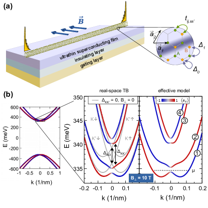
Figure 1: Set-up and bulk properties of a proximitized nanotube. (a) Schematic of the system, the CNT with its proximal superconductor and a gating layer. A magnetic field is applied in parallel to the substrate and perpendicular to the nanotube. We find Majorana quasiparticles at the ends of the CNT/superconductor hybrid. The ingredients of our model are shown in the inset. The nearest neighbor hopping $t_{ij,ss^{\prime}}$ is spin-dependent because of spin-orbit coupling. The superconducting substrate (i) breaks the rotational symmetry of the nanotube, as shown by the darker strip with finite electrostatic on-site potential, and (ii) induces superconducting pairing in the nanotube, with on-site ($\Delta_{0}$) and nearest-neighbor ($\Delta_{1}$) pairing correlations. (b) The energy bands of a (12,4) nanotube in the vicinity of the Dirac points are shown in the leftmost plot, with red/blue corresponding to spin up/down (quantized along the nanotube axis) bands. Our region of interest here is the neighborhood of the $\Gamma$ point in the conduction band. The enlarged plots show the spectrum in this region, obtained both in the real-space tight-binding calculation and in an analytical effective model. The spin-orbit splitting between the Kramers doublets at $k=0,B_{\perp}=0$ is $\Delta_{\mathrm{SO}}$ (here equal 2 meV), and the width of the anticrossing opening between different valley states is $\Delta_{KK^{\prime}}$ (here 2.5 meV). Grey lines shown in the plot correspond to subbands without the valley mixing. There we can assign spin and valley quantum number to each band. With the valley mixing, $B_{\perp}$ is able to open a gap at $k=0$.

II Set-up and bulk properties

Carbon nanotubes can be regarded as graphene sheets rolled into seamless cylinders. The rolling direction is described by the so-called chiral indices of the CNT, $(n,m)$ Saito et al. (1998). The bulk spectrum of the CNT consists of 1D subbands created by cutting graphene’s dispersion by lines of constant angular momentum, determined by the periodic boundary conditions around the circumference. The electronic properties of the nanotube depend strongly on the rolling direction, which decides whether the subbands cross the Dirac points or not. If they do, i.e. when $(n-m)|\mathrm{mod}\,3=0$ the nanotubes are metallic and the lowest 1D conduction bands descend deeply towards the apex of graphene’s Dirac cones, reaching Fermi velocities of the order of $10^{6}$ m/s. If $(n-m)|\mathrm{mod}\,3\neq 0$, the CNT is semiconducting and the lowest bands lie higher up on the Dirac cones and are much flatter, with Fermi velocities dependent on the chemical potential, but typically not higher than $\sim 10^{3}$ m/s. In the following we shall use for illustration a finite (12,4) CNT, although we find the same topological phases in semiconducting nanotubes of other chiralities, in different parameter regimes.
The microscopic model of the nanotube which we use, with one $p_{z}$ orbital per atomic site, is shown schematically in Fig. 1(a). The tiny spin-orbit coupling of graphene becomes significantly enhanced in carbon nanotubes due to the curvature of their atomic lattice Ando (2000); Kuemmeth et al. (2008); Izumida et al. (2009). It defines a quantization axis for the spin, along the CNT axis, and induces a band splitting $\Delta_{SO}$, which is reported to reach values larger than 3 meV Steele et al. (2013). The resulting low energy band structure for a (12,4) semiconducting nanotube is shown in the small panel of Fig. 1b) and, zoomed up around the $\Gamma$ point, with the grey lines in the larger panel. The band crossing at $k=0$ is protected by symmetry since the crossing bands belong to different valleys $K$ and $K^{\prime}$, i.e. in this CNT to different angular momenta Marganska et al. (2015); Izumida et al. (2016), and the magnetic field cannot hybridize them. The presence of a superconducting substrate plays here a double role. On the one hand it serves as a source of superconducting correlations in the nanotube, acquired by the proximity effect. On the other hand it breaks the rotational symmetry of the nanotube and is the cause of valley mixing $\Delta_{KK^{\prime}}$. In combination with the perpendicular magnetic field $B_{\perp}$, this allows the bands at the $\Gamma$ point to hybridize. The increased electrostatic potential in the vicinity of the substrate atoms is shown as a darker stripe across the inset in Fig. 1(a). The real space CNT Hamiltonian in the presence of perpendicular magnetic field $B_{\perp}$ is then given by

$$\begin{split}H_{0}&=\sum_{\langle i,j\rangle,ss^{\prime}}t_{ij,ss^{\prime}}c_{is}^{\dagger}c_{js^{\prime}}^{\vphantom{{\dagger}}}+\sum_{i,s}V(\varphi_{i})c_{is}^{\dagger}c_{is}^{\vphantom{{\dagger}}}\\ &+\mu_{B}B_{\perp}\sum_{i,s}c_{is}^{\dagger}c_{i,-s}^{\vphantom{{\dagger}}},\end{split}$$ (1)

where $i$ indexes the atomic positions, $s$ is the spin, $t_{ij,ss^{\prime}}$ is the spin-dependent nearest neighbor hopping Ando (2000), $\langle i,j\rangle$ denotes a sum over the nearest neighbor atoms, and $V(\varphi_{i})$ is the potential induced by the substrate at the $i$-th nanotube atom. It depends on the atom’s height above the substrate, i.e. on its angular coordinate $\varphi_{i}$. The resulting band structure is shown in the left large panel of Fig. 1(b), featuring both the helical, spin-momentum locked modes and two energy ranges with odd number of Fermi surfaces. We have also constructed a four-band effective model in the reciprocal space (detailed discussion follows in the Methods section), with the band structure shown also in Fig. 1(b). A very good agreement with the spectrum obtained from the full tight-binding calculation is achieved, which is crucial in the studies of topological matter.
When the substrate turns superconducting, it induces Cooper pairing in the nearby normal system. We propose to use the two-dimensional (2D) gate-tunable superconductor NbSe₂, where superconductivity can survive up to 30 T in magnetic fields applied in-plane Xi et al. (2016). Hence in our set-up the magnetic field is applied in the direction perpendicular to the nanotube axis but, crucially, parallel to the substrate. We treat the superconducting correlations in the spirit of Ref. Uchoa and Castro Neto (2007), admitting both the on-site and nearest-neighbor pairing $\Delta_{0}$ and $\Delta_{1}$. With the superconducting pairing the system is described by

$$H = H_{0}-\mu\sum_{i,s}c_{is}^{\dagger}c_{is}^{\vphantom{{\dagger}}}+\sum_{i,s}(\Delta_{0}c_{is}^{\dagger}c_{i,-s}^{\dagger}+\mathrm{h.c.})$$ (2)

$$+\sum_{\langle i,j\rangle,s}(\Delta_{1}c_{is}^{\dagger}c_{j,-s}^{\dagger}+\mathrm{h.c.}),$$

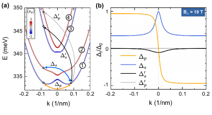
Figure 2: Superconducting pairing between the four bands. (a) The energy bands colored by their expectation value of $s_{x}$, spin in the direction of the field. The superconducting pairing couples all four bands. The pairings between a positive momentum state in band ➀ and its negative momentum partners in all bands are indicated. Their strength depends on the value of $B_{\perp}$. (b) The s-like pairings are even in $k$, the p-like pairings are odd.

where energies are measured from the chemical potential $\mu$, controlled e.g. by a gating layer beneath the substrate. The $\Delta_{1}$ contribution is not necessary for the MQPs to arise and we shall discuss its effects further only in last section of the Supplemental Material, here assuming $\Delta_{0}\in\mathbb{R}$ and $\Delta_{1}=0$. In the effective model, whose construction is described in the Methods section, the superconducting pairing from (2) couples all four single-particle bands as shown in Fig. 2(a), with some pairing terms having an s-wave and some a p-wave symmetry, visible in Fig. 2(b).
In order to find its spectrum, we express the Hamiltonian (2) in a particle-hole symmetric form by introducing a Nambu spinor, $\Psi=\oplus_{i=1}^{N}\Psi_{i},\quad\Psi_{i}^{\dagger}=(c_{i\uparrow}^{\dagger},c_{i\downarrow}^{\dagger},c_{i\uparrow},c_{i\downarrow})$, where $\oplus$ is the direct sum over the $N$ atomic positions. This procedure effectively doubles the number of degrees of freedom of the system. The full Hamiltonian becomes $H=\frac{1}{2}\Psi^{\dagger}H_{\mathrm{BdG}}\Psi$, where the field operators are contained in $\Psi,\Psi^{\dagger}$ and $H_{\mathrm{BdG}}$ is an ordinary matrix, the Bogoliubov-de Gennes Hamiltonian of our system. Its eigenvectors, defining the quasiparticle eigenstates with a set of quantum numbers $n$, have the structure

$$\boldsymbol{\chi}^{n}=\oplus_{i=1}^{N}\boldsymbol{\chi}^{n}_{i},\quad(\boldsymbol{\chi}^{n}_{i})^{T}=(u^{n}_{i\uparrow},u^{n}_{i\downarrow},v^{n}_{i\uparrow},v^{n}_{i\downarrow}),$$ (3)

where $n$ is a generic collective index which may contain e.g. the valley and, in a system with translational invariance, $k$ quantum numbers. The particle components with spin $s$ on atom $i$ are denoted by $u^{n}_{is}$ and the corresponding hole components by $v^{n}_{is}$. The quantum eigenstates of the system have the form $|\psi^{n}\rangle=\oplus_{i=1}^{N}\Psi_{i}^{\dagger}\cdot\chi^{n}_{i}\,|0\rangle_{\mathrm{BCS}}$, where $|0\rangle_{\mathrm{BCS}}$ is the BCS ground state in the CNT. The low energy bands obtained for our proximitized infinite (12,4) nanotube are shown in Fig. 3, for the three topologically distinct phases encountered by increasing the magnetic field. The color scale shows the overall weight of particle component in the given energy eigenstate, $|u|^{2}=\sum_{is}|u_{is}|^{2}$. The solutions which have a predominantly particle character trace the original single-particle bands, while the predominantly hole-type solutions are mirror-reflected around the chemical potential.

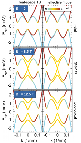
Figure 3: The Bogoliubov-de Gennes spectra of the superconducting nanotube in three different topological phases which can be accessed by tuning $B_{\perp}$. The color scale shows the weight of the particle part of the corresponding CNT’s eigenstate; gold color indicates equal particle and hole contributions. The superconducting pairing is $\Delta_{0}=0.4$ meV, $\Delta_{1}=0$.

III Symmetries and topological invariants

The Hamiltonian $H_{\mathrm{BdG}}$, like all Bogoliubov-de Gennes Hamiltonians, is by construction invariant under a particle-hole operation. That is, we can define an antiunitary operator $\mathcal{P}$, such that $\mathcal{P}H_{\mathrm{BdG}}\mathcal{P}^{-1}=-H_{\mathrm{BdG}}$. The action of $\mathcal{P}$ on the original electron operators and on doubled Hilbert space states is

$$\mathcal{P}c_{is}=c_{is}^{\dagger},\quad\mathcal{P}\boldsymbol{\chi}_{i}=(v_{i\uparrow}^{*},v_{i\downarrow}^{*},u_{i\uparrow}^{*},u_{i\downarrow}^{*})^{T}.$$ (4)

The particle-hole operation maps the positive energy solutions onto their Nambu partners with negative energy. If the particle-hole symmetric Hamiltonian of a finite system has zero energy modes, they can be cast in the form of eigenstates of $\mathcal{P}$,

$$\mathcal{P}\psi=\psi.$$ (5)

Inspecting the first relation of (4) shows that (5) is only an equivalent definition of the Majorana property, usually stated as $\gamma_{\sigma}(\boldsymbol{r})=\gamma^{\dagger}_{\sigma}(\boldsymbol{r})$, where $\gamma^{\dagger}$ is the operator creating a particle with spin $\sigma$ at position $\boldsymbol{r}$.
The presence or absence of Majorana solutions can be predicted from a topological phase diagram, where different phases correspond to different values of a topological invariant. In a system with translational symmetry, such as the bulk of the CNT, the basic quantity determining the topological invariant in 1D is $\gamma^{-}$, the sum of the Berry phases carried by all occupied (negative energy) bands, integrated over the Brillouin zone. Since $\gamma^{-}$ is gauge-dependent and defined only up to an integer, another invariant is commonly used, $W=\exp(i2\pi\gamma^{-})$, which is gauge-independent. The particle-hole symmetry in a system with translational invariance is expressed as $\mathcal{P}H_{\mathrm{BdG}}(k)\mathcal{P}^{-1}=-H_{\mathrm{BdG}}(-k)$ Chiu et al. (2016); Sato and Ando (2017), i.e. the positive energy solutions at momentum $k$ are related to negative energy solutions at momentum $-k$, as sketched in Fig. 4(a). This constrains the values which $W$ can take to $\pm 1$, i.e. $W$ is of a $\mathbb{Z}_{2}$ type, associated with the Altland-Zirnbauer D class systems Chiu et al. (2016); Sato and Ando (2017). $W=+1$ corresponds to the trivial topological phase, while $W=-1$ implies the presence of MQPs at the system boundaries. The phase diagram calculated for our model nanotube, using the standard Pfaffian technique Chiu et al. (2016); Sau and Tewari (2013) and the effective model for the bulk bands, is shown in Fig. 4(b). The borders between different phases in the diagram correspond to $(B_{\perp},\mu)$ such that the gap is closed at $k=0$. From our effective four-band model we find that this occurs at

$$\tilde{\mu}^{2} = \Delta_{\mathrm{SO}}^{2}+4(\Delta_{KK^{\prime}}^{2}+(\mu_{B}B_{\perp})^{2}-\Delta_{0}^{2})$$ (6)

$$\pm\sqrt{4\Delta_{KK^{\prime}}^{2}((\mu_{B}B_{\perp})^{2}-\Delta_{0}^{2})-\Delta_{0}^{2}\Delta_{\mathrm{SO}}^{2}},$$

where $\tilde{\mu}$ is the chemical potential measured from the center of either the ➀,➁ or ➂,➃ pair in Fig. 1(b). The critical magnetic field is given by $\mu_{B}B_{c}=2\Delta_{0}\Delta_{KK^{\prime}}/\sqrt{\Delta_{SO}^{2}+4\Delta_{KK^{\prime}}^{2}}$. If we assume that the band pair ➀,➁ is independent of ➂,➃, we can expand (6) around $B_{c}$, obtaining a simpler formula $\tilde{\mu}^{2}=\Delta_{0}^{2}((B_{\perp}/B_{c})^{2}-1)$. The red lines in Fig. 4(b) follow (6), the dashed lines mark the borders of the non-trivial phase obtained with the simpler approximated formula. The coupling between the band pairs changes visibly the phase diagram – when the Zeeman energy reaches the magnitude of the original spin-orbit splitting, it destroys the topological phase. The same phenomenon occurs in multiband semiconducting nanowires, where the mixing between various transverse modes caused by the Rashba spin-orbit coupling strongly reduces the non-trivial topological regions in the phase diagram  Stanescu and Tewari (2013); Lutchyn and Fisher (2011); Lim et al. (2012).

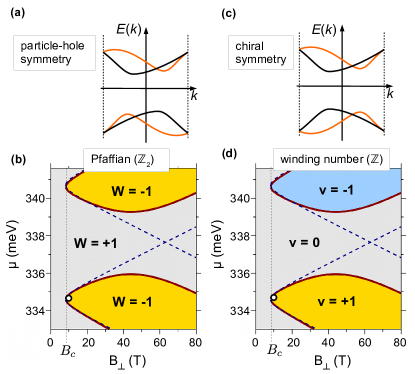
Figure 4: Symmetries and topological invariants. (a) Sketch of a spectrum with particle-hole symmetry. Bands of the same color are related by the symmetry. (b) The phase diagram calculated using the effective model and the Pfaffian formulation of the topological invariant, typical for particle-hole symmetric systems. The topologically non-trivial regions are shown in yellow, the red line at the border between the phases is the contour of $E=0$ at the $\Gamma$ point. The dot in the lower $W=-1$ area marks the $\mu$ and $B_{\perp}$ used in Fig. 6. The dashed lines trace the borders of non-trivial phase calculated from a model which contains only one single-particle band pair, either ➀ and ➁ (higher region) or ➂ and ➃ (lower region) from Fig. 1b. (c) Sketch of a spectrum with chiral symmetry. The Bogoliubov-de Gennes spectrum in Fig. 3 has both particle-hole and chiral symmetry. (d) The phase diagram calculated using the winding number invariant, defined for chiral- symmetric systems. The values $\nu=\pm 1$ in the lower and upper non-trivial area indicate that these regions correspond to different topological phases, with one zero energy mode in each.

As can be seen in Fig. 3, the Hamiltonian $H_{\mathrm{BdG}}$ is highly symmetric. In particular, a unitary operation $C$ can be defined, such that $CH_{\mathrm{BdG}}(k)C^{-1}=-H_{\mathrm{BdG}}(k)$. The operation $C$ is a so-called chiral symmetry, connecting positive and negative energy solutions at the same momentum $k$, as sketched in Fig. 4(c). The MQPs in our system are also eigenstates of $C$. In systems with this symmetry, the topological invariant $\gamma^{-}$ has a clear interpretation as a winding number, $\gamma^{-}=\nu/2$ Izumida et al. (2017). The winding number is an integer, i.e. it belongs to $\mathbb{Z}$. That apparent contradiction with $W\in\mathbb{Z}_{2}$ is solved when we recall that $W$ was constructed with an extra exponentiation step, which obliterates the difference between the phases with $\nu=\pm 1$. The phase diagram calculated using the winding number is shown in Fig. 4(d), with exactly the same phase boundaries, but showing clearly that the lower non-trivial region and the upper non-trivial region in fact correspond to different non-trivial phases. Further discussion on this subject can be found in Sec. IV of the Supplemental Material.
With both the particle-hole $\mathcal{P}$ and the chiral $C$ symmetries, the Hamiltonian is also invariant under a product of both, i.e. $\tilde{\mathcal{T}}=C\mathcal{P}^{-1}$. This symmetry is antiunitary and commutes with the Hamiltonian, $\tilde{\mathcal{T}}H_{\mathrm{BdG}}(k)\tilde{\mathcal{T}}^{-1}=H_{\mathrm{BdG}}(-k)$, similar to the time-reversal. Contrary to the true time-reversal operation which in systems with half-integer spin squares to $-1$, here $\tilde{\mathcal{T}}^{2}=+1$, placing our nanotube not in the D, but in the BDI class with the winding number as an integer topological invariant.

IV Emergence of MQPs in finite nanotubes

Changing the chemical potential or the strength of the magnetic field can drive the proximitized nanotube across a topological phase transition, into a regime in which it becomes a topological superconductor. An example of the changes in the Bogoliubov-de Gennes spectrum during such a transition is shown in Fig. 5(a), for a 6 $\mu$m long (12,4) CNT at a fixed chemical potential $\mu=334.6$ meV and varying magnetic field $B_{\perp}$. The energy of the lowest quasiparticle states is further lowered with increasing $B_{\perp}$, until they become a doubly degenerate zero energy mode. The degeneracy is artificial, caused by the doubling of degrees of freedom introduced with the Nambu spinor, and the nanotube de facto hosts only one eigenstate at zero energy. The change in the shape of the quasiparticle wave function associated with the lowest energy eigenstate is illustrated in Fig. 5(b), showing clearly its increasing localization at the ends of the proximitized CNT. In the figure only the amplitude $|u_{\uparrow}(\boldsymbol{r})|$ of the particle component with spin up is shown, the remaining components $u_{\downarrow}(\boldsymbol{r}),v_{\uparrow}(\boldsymbol{r}),v_{\downarrow}(\boldsymbol{r})$ have profiles which are indistinguishable from $|u_{\uparrow}(\boldsymbol{r})|$ at this scale. Having a direct access to the particle and hole components of the zero energy mode, we can prove that it indeed has Majorana nature according to (5).

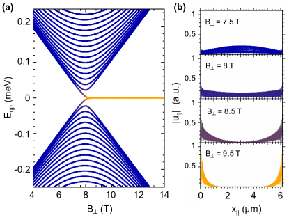
Figure 5: Topological phase transition. (a) The quasiparticle spectrum of a finite (12,4) nanotube with 4000 unit cells ($L=6.03\,\mu$m), at the chemical potential $\mu=334.6$ meV for varying magnetic field. The topological phase transition occurs at $B_{c}=8.5$ T, beyond which the lowest energy eigenstate becomes a zero energy mode. (b) The wave function of the lowest energy mode undergoes a gradual localization with increasing magnetic field. Here only the amplitude $|u_{\uparrow}(x_{\parallel})|$ of the spin up particle component, projected onto the direction along the CNT’s axis, is shown. The shape of the remaining components is indistinguishable from that of $|u_{\uparrow}(x_{\parallel})|$ at this scale, which comprises the data points from $N=8.32\cdot 10^{5}$ atoms. The units are arbitrary and the same for all wave function plots in this figure.

The spatially resolved wave function of the zero energy mode at $B_{\perp}=9.5$ T is shown in Fig. 6(a). The amplitude of spin up and down particle components, $|u_{\uparrow}(\boldsymbol{r})|$ and $|u_{\downarrow}(\boldsymbol{r})|$, is shown both as the distance from the CNT’s surface (grey) at each atomic position and via the color scale. The wavelength of the oscillations is set by the value of $k_{F}$ at the chosen chemical potential. The decay length is field-dependent and at $B_{\perp}=9.5$ it is $\sim 0.4\,{\mathrm{\mu m}}$. The Majorana nature of the zero energy mode becomes evident in the Fig. 6(b), where the differences between particle and (complex conjugated) hole component of the wave function for each spin, $|u_{\uparrow}(\boldsymbol{r})-v^{*}_{\uparrow}(\boldsymbol{r})|$ and $|u_{\downarrow}(\boldsymbol{r})-v^{*}_{\downarrow}(\boldsymbol{r})|$ are shown. They are identical up to the order of $10^{-5}$ of the maximum amplitude, which constitutes a numerical proof that the zero energy mode fulfills the Majorana condition (5).

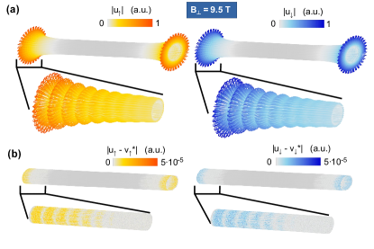
Figure 6: Majorana bound states. (a), The full spatial profile of the the spin up and spin down particle components, $|u_{\uparrow}(\boldsymbol{r})|$ and $|u_{\downarrow}(\boldsymbol{r})|$. The amplitude of the electronic wave function is shown through both the distance from the nanotube’s surface (light grey) and through the color scale. The wavelength of the oscillations is given by the value of $k_{F}$ at the chosen chemical potential. (b), Spatially resolved amplitude of the difference between the particle and conjugated hole components for the same spin, $|u_{\uparrow}(\boldsymbol{r})-v^{*}_{\uparrow}(\boldsymbol{r})|$ and $|u_{\downarrow}(\boldsymbol{r})-v^{*}_{\downarrow}(\boldsymbol{r})|$. The distance from the CNT’s surface is scaled in the same way as in c, and the color scale is greatly enhanced. Only faint differences are visible, of the order of $10^{-5}$, which shows the Majorana nature of the zero energy mode.

V MQP stability and experimental feasibility

The stability of the MQPs against perturbations is crucial for their experimental realization. The techniques for growing carbon nanotubes are now so advanced that their atomic lattices are nearly perfect Cao et al. (2005). We have analyzed our model nanotube at several low concentrations of impurities and found that the Majorana mode is remarkably stable (cf. Sec. VI of the Supplemental Material). Another factor which has to be taken into account is the precision of alignment of the magnetic field. The presence of a field component parallel to the nanotube axis gives rise to the Aharonov-Bohm effect. In nanotubes this causes a different orbital response in the two valleys, resulting in a removal of the valley degeneracy Ajiki and Ando (1993) and breaking of the chiral symmetry. When the parallel component of the magnetic field reaches a threshold value, the electrons on opposite sides of the $\Gamma$ point no longer have matching momenta and the superconducting correlations become ineffective, yielding a gapless spectrum. The lowest thirty two eigenvalues of the Bogoliubov-de Gennes spectrum in magnetic field of 12 T amplitude and varying angle $\theta$ with respect to the nanotube axis are plotted in Fig. 7. At this chosen field amplitude the finite system supports a Majorana mode within a range of $\pm 5^{\circ}$ deviation of the field from the perpendicular. Increasing the field amplitude widens the maximum gap at 90^∘, but the higher value of the parallel component decreases the $\theta$ range in which the spectrum is gapped.
The two major experimental challenges in achieving the formation of MQPs in this setup are the necessity of controlling the chemical potential of the CNT and of applying a large magnetic field without destroying superconducting correlations. Both may be accomplished with the use of 2D transition metal dichalcogenide (TMDC) superconductors, such as NbSe₂, with its larger superconducting gap of 1.26 meV Huang et al. (2007). The superconducting pairing was demonstrated to survive in fields up to 30 T Xi et al. (2016), and the thinness of the 2D layer allows the superconductor itself to be gated, together with the CNT in its proximity. Thus the goal of tuning a CNT into the non-trivial topological regime, with its attendant Majorana boundary modes, is within the reach of state-of-the-art technology.

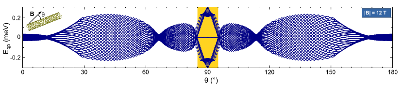
Figure 7: Stability of MQPs with respect to magnetic field alignment. The thirty two lowest quasiparticle energies as a function of varying angle of the magnetic field, with its amplitude fixed at $B=12$ T. The bulk Hamiltonian is gapped only within the area marked in yellow, $85^{\circ}\leq\theta\leq 95^{\circ}$. In a finite system a zero energy mode appears throughout this range of $\theta$, with maximum distance to the other eigenstates at $\theta=90^{\circ}$.

Appendix A Tight-binding model

The model is constructed for one $p_{z}$ orbital per atomic site. The hopping matrix elements, taking into account the hybridization between $\sigma$ and $\pi$ orbitals and the spin-orbit coupling induced by the curvature, are given by the formulae in Refs. Ando (2000); del Valle et al. (2011). In our calculations we chose $V_{pp}^{\sigma}=6.38$ eV and $V_{pp}^{\pi}=-2.66$ eV after Ref. Tománek and Louie, 1988, and we set the small parameter controlling nanotube’s spin-orbit coupling to $\delta_{SO}=3\cdot 10^{-3}$, similar to $2.8\cdot 10^{-3}$ measured in Ref. Jhang et al., 2010. The electrostatic potential of the substrate is taken here to be a continuous ridge, adding an on-site potential term to the Hamiltonian of the CNT at the atomic sites in the proximity of the superconducting substrate. We have tested several shapes of this ridge with similar values of the resulting valley mixing energy scale, $\Delta_{KK^{\prime}}$. For all calculations presented here we chose a Gaussian form of $V(\varphi)$,

$$V(\varphi)=V_{0}\,\exp(-(\varphi-\varphi_{0})^{2}/\Delta\varphi^{2}),$$ (7)

where $\varphi$ is the angular coordinate of the nanotube atom, $V_{0}$ is an arbitrarily chosen maximum height of the substrate’s potential, $\varphi_{0}$ is the shift between nanotube coordinates and the CNT-S contact line, and $\Delta\varphi$ controls the sharpness of the potential (more details can be found in Sec. I of the Supplemental Material). In the calculations we assumed $V_{0}=0.4$ eV, $\varphi_{0}=90^{\circ}$ and $\Delta\varphi=2.5^{\circ}$.

Appendix B Effective four-band model

The Hamiltonian of a CNT in the reciprocal space is obtained using a zone folding technique. The spectrum of the CNT is follows from that of graphene by imposing the periodic boundary conditions on the value of transverse momentum, turning the 2D dispersion of graphene into a series of 1D cuts, which are the CNTs one-dimensional subbands Saito et al. (1998). When the curvature of the CNT’s lattice is included, it results in both spin-dependent and spin-independent modifications of graphene’s dispersion. They are most significant near the Dirac points of the spectrum. In models treating one $p_{z}$ orbital per atomic site their effects can be incorporated in the dispersion as shifts in both transverse and longitudinal momentum. The low energy electronic spectrum of a CNT in the conduction band for given transverse momentum $k_{\perp}$ and longitudinal momentum $k$ is then given by

$$\varepsilon_{\tau\sigma}\left(k_{\perp},k\right) = \hbar v_{F}\left\{\left(k-\tau K_{\parallel}+\tau\Delta k_{\parallel}^{c}\right)^{2}\right.$$

$$+\left.\left(k_{\perp}-\tau K_{\perp}+\tau\Delta k_{\perp}^{c}+s\Delta k_{\perp}^{\mathrm{SO}}\right)^{2}\right\}^{1/2},$$

where $K_{\perp},K_{\parallel}$ are the transverse and longitudinal component of momentum at the Dirac point $K$. The quantum numbers $\tau$ and $s$ stand for the valley ($K:\;\tau=1$, $K^{\prime}:\;\tau=-1$) and the spin component along the CNT axis $s=\pm 1$. All quantities in this dispersion are directly related to the hopping integrals across $\pi$ ($V_{pp}^{\pi})$ and $\sigma$ bonds ($V_{pp}^{\sigma}$) in graphene, to nanotube geometry and to carbon’s intrinsic spin orbit coupling Ando (2000); del Valle et al. (2011), and their values and signs may vary, depending on which set of tight-binding parameters is used. The numerical values of those momentum shifts in our calculations are $\Delta k_{\perp}^{c}=-22.83\,\mu\mathrm{m}^{-1}$, $\Delta k_{\parallel}^{c}=66.62\,\mu\mathrm{m}^{-1}$ and $\Delta k_{\mathrm{SO}}=-2.917\,\mu\mathrm{m}^{-1}$. In the case of our (12,4) semiconducting nanotube $K_{\parallel}=0$ and the lowest energy subbands shown in Fig. 1b have $k_{\perp}-\tau K_{\perp}=\tau/3R$. In the following we shorten the notation by setting $k_{\perp}=K_{\perp}+1/3R$ and omitting it from the argument of $\varepsilon_{\tau s}(k_{\perp},k)$. The spin-orbit splitting $\Delta_{\mathrm{SO}}$ from the main text is then $\Delta_{\mathrm{SO}}=\varepsilon_{K\uparrow}(0)-\varepsilon_{K\downarrow}(0)$. Note that the single-particle energies satisfy the time-reversal conjugation, $\varepsilon_{\tau s}\left(k\right)=\varepsilon_{-\tau-s}\left(-k\right)$.
With added valley-mixing induced by the superconducting substrate and in an external perpendicular magnetic field the CNT is described by the following effective Hamiltonian :

$$H=H_{\text{CNT}}+H_{\Delta_{KK^{\prime}}}+H_{\text{Z}}\text{.}$$ (9)

The effective Hamiltonian in second quantization for the CNT including a reference chemical potential $\mu$ is given by

$$H_{\text{CNT}}-\mu N=\sum_{k,\tau,s}\xi_{\tau s}\left(k\right)c_{k\tau s}^{\dagger}c_{k\tau s}\text{,}$$ (10)

where $\xi_{\tau s}\left(k\right)$ is the single-particle energy measured with respect to the chemical potential, $\xi_{\tau s}\left(k\right)=\varepsilon_{\tau s}\left(k\right)-\mu$. We model the $k$ dependence of the valley mixing potential (see Sec. I of the Supplemental Material for details) by modifying the longitudinal curvature shift and fitting an appropriate constant $\Delta_{KK^{\prime}}$ to the band structure obtained from the real space calculation. In our case $\varepsilon_{\tau s}\left(k\right)=\hbar v_{F}\sqrt{\left(k+0.8\tau\Delta k_{\parallel}^{c}\right)^{2}+\left(1/3R+\Delta k_{\perp}^{c}+\tau s\Delta k_{\perp}^{SO}\right)^{2}}$. The valley-mixing term $H_{\Delta_{KK^{\prime}}}$ couples two electron states at opposite valleys but with the same spin $s$ and becomes

$$H_{\Delta_{KK^{\prime}}}=\sum_{k,s}\Delta_{KK^{\prime}}c_{kKs}^{\dagger}c_{kK^{\prime}s}+\Delta_{KK^{\prime}}^{\star}c_{kK^{\prime}s}^{\dagger}c_{kKs}\text{,}$$ (11)

with $\Delta_{KK^{\prime}}\in\mathbb{C}$. In our calculations $\Delta_{KK^{\prime}}$ is real and equal to 2.5 meV. The Zeeman energy $H_{\text{Z}}$ due to the perpendicular magnetic field $B_{\perp}$ induces a coupling of electrons with opposite spins and in the same valley

$$H_{Z}=\mu_{B}B_{\perp}\sum_{k,\tau}c_{k\tau\uparrow}^{\dagger}c_{k\tau\downarrow}+c_{k\tau\downarrow}^{\dagger}c_{k\tau\uparrow}\text{,}$$ (12)

i.e. we assume $B_{\perp}$ to be applied in the $x$ direction, while the $z$ direction runs along the CNT axis. The eigenstates of the resulting Hamiltonian are then in general linear combinations of all $\tau,s$ eigenstates of the original $H_{\text{CNT}}$. We denote them by ➀,➁,➂,➃, shown in Fig. 1b.

The superconducting correlations induced by proximity are treated in a mean-field approximation. We only consider the case of an on-site pairing potential which is described by the superconducting gap $\Delta_{0}$. Since $\Delta_{0}$ is isotropic in momentum space, our mean-field pairing Hamiltonian has an s-wave gap symmetry. The mean-field Hamiltonian reads

$$H_{\text{SC}}=\sum_{k}\Delta_{0}\left(c_{kK\uparrow}^{\dagger}c_{-kK^{\prime}\downarrow}^{\dagger}+c_{kK^{\prime}\uparrow}^{\dagger}c_{-kK\downarrow}^{\dagger}+\mathrm{h.c.}\right)\text{,}$$ (13)

where we are coupling the corresponding Kramers partners. Introducing the Nambu spinor defined as

$$\Psi^{\dagger}=(c_{kK\uparrow}^{\dagger},c_{kK\downarrow}^{\dagger},c_{kK^{\prime}\uparrow}^{\dagger},c_{kK^{\prime}\downarrow}^{\dagger},c_{-kK^{\prime}\downarrow},c_{-kK^{\prime}\uparrow},c_{-kK\downarrow},c_{-kK\uparrow}),$$

we obtain the Bogoliubov-de Gennes (BdG) Hamiltonian

$$\mathcal{H}_{\mathrm{BdG}}(k)=\begin{pmatrix}H(k)&\Delta\\ -\Delta&-H(-k)\end{pmatrix},$$ (14)

with

$$H(k)=\begin{pmatrix}\xi_{K\uparrow}(k)&\mu_{B}B_{\perp}&\Delta_{KK^{\prime}}&0\\ \mu_{B}B_{\perp}&\xi_{K\downarrow}(k)&0&\Delta_{KK^{\prime}}\\ \Delta_{KK^{\prime}}&0&\xi_{K^{\prime}\uparrow}(k)&\mu_{B}B_{\perp}\\ 0&\Delta_{KK^{\prime}}&\mu_{B}B&\xi_{K^{\prime}\downarrow}(k)\end{pmatrix},$$ (15)

and

$$\Delta=\begin{pmatrix}-\Delta_{0}&&&\\ &\Delta_{0}&&\\ &&-\Delta_{0}&\\ &&&\Delta_{0}\\ \end{pmatrix}.$$

The single particle energies are defined with respect to the chemical potential $\mu$, as in (10). The resulting p-wave and s-wave components of the pairing Hamiltonian in the eigenbasis of the ➀,➁,➂ and ➃ are shown in Fig. 2 and discussed further in Sec. II of the Supplemental Material. A detailed analysis of the superconducting pairing, also within an effective two-band model can be found in Sec. III of the Supplemental Material.

Appendix C Gap closing condition

The Hamiltonian $\mathcal{H}_{\mathrm{BdG}}(k)$ has a chiral symmetry, i.e. there exists a unitary operator $C$ such that $C\mathcal{H}_{\text{BdG}}\left(k\right)C^{-1}=-\mathcal{H}_{\text{BdG}}\left(k\right)$. In the basis in which the operator $C$ is diagonal (details can be found in the next section), the BdG Hamiltonian is given by

$$\mathcal{H}^{C}_{\text{BdG}}\left(k\right)=\begin{pmatrix}0&D\left(k\right)\\ D^{\dagger}\left(k\right)&0\end{pmatrix}\text{,}$$

where $D(k)=H(k)-i\Delta$. In order to obtain the gap closing condition we square the BdG Hamiltonian in chiral basis, which yields

$$\left(\mathcal{H}^{C}_{\text{BdG}}\left(k\right)\right)^{2}=\begin{pmatrix}D\left(k\right)D^{\dagger}\left(k\right)&0\\ 0&D^{\dagger}\left(k\right)D\left(k\right)\end{pmatrix}\text{.}$$

This matrix has zero energy eigenvalues at the $\Gamma$ point if $\det\left(D\left(k=0\right)D^{\dagger}\left(k=0\right)\right)=\det\left(D^{\dagger}\left(k=0\right)D\left(k=0\right)\right)=0$. From this we obtain the exact gap closing condition at the $\Gamma$ point, given by Eq. (6).

Appendix D Topological invariants.

The symmetries of the BdG Hamiltonian  (14) can be expressed in terms of Pauli matrices, denoted by $\pi$ in the particle-hole (Nambu) subspace, by $\tau$ in the valley subspace and by $s$ in the spin subspace. The particle-hole symmetry operator $\mathcal{P}$, such that $\mathcal{P}\mathcal{H}_{\mathrm{BdG}}(k)\mathcal{P}^{-1}=-\mathcal{H}_{\mathrm{BdG}}(-k)$, is given by $\mathcal{P}=\pi_{x}\otimes\tau_{x}\otimes s_{x}\,\mathcal{K}$, where $\tau_{0}$ and $s_{0}$ are the identities in their respective subspaces and $\mathcal{K}$ denotes the operator of the complex conjugation. The Hamiltonian $H_{\mathrm{BdG}}$ has also a chiral symmetry, i.e. it fulfills $C\mathcal{H}_{\mathrm{BdG}}(k)C^{-1}=-\mathcal{H}_{\mathrm{BdG}}(k)$ with a unitary operator $C$. The operator is given by $C=\pi_{y}\otimes\tau_{0}\otimes s_{0}$. The presence of those two symmetries implies that there exists a third one, which we call $\tilde{\mathcal{T}}=C\mathcal{P}^{-1}$ and which fulfills $\tilde{\mathcal{T}}\mathcal{H}_{\mathrm{BdG}}(k)\tilde{\mathcal{T}}^{-1}=\mathcal{H}_{\mathrm{BdG}}(-k)$. Its expression in this basis is $\tilde{\mathcal{T}}=-i\pi_{z}\otimes\tau_{x}\otimes s_{x}\,\mathcal{K}$. The operation $\tilde{\mathcal{T}}$ squares to $+1$, hence it is clear that it is not the time reversal symmetry of a spin-1/2 system. The fact that it is diagonal in the Nambu space implies that already the non-superconducting Hamiltonian $H(k)$ (15) is invariant under a restricted $\tilde{\mathcal{T}}_{\mathrm{red}}=\tau_{x}\otimes s_{x}\mathcal{K}$, which is indeed the case and reflects a physical symmetry of the system. It is the symmetry of rotation with respect to an axis perpendicular to the CNT, which exchanges both the valley, longitudinal momentum and spin. It also exchanges the sublattices, which accounts for its $\mathcal{K}$ component. If, and only if, the magnetic field is also applied perpendicular to the CNT axis, the non-superconducting Hamiltonian is invariant under $\tilde{\mathcal{T}}_{\mathrm{red}}$.
Pfaffian $(\mathbb{Z}_{2})$ invariant. In systems with particle-hole symmetry the topological invariant $W$ can be evaluated using the representation of the Hamiltonian in the Majorana basis, i.e. the basis of eigenstates of $\mathcal{P}$ Chiu et al. (2016), obtained by a transformation $U_{M}$, $\mathcal{H}_{M}(k)=U_{\mathrm{M}}\mathcal{H}_{\mathrm{BdG}}(k)U_{\mathrm{M}}^{\dagger}$. We can define a matrix $X$ by $iX(k)=\mathcal{H}_{M}(k)$. At the time reversal invariant momenta $k=0,\pi/a$, $X(k)$ is a real and skew symmetrix matrix, $X(k)=-[X(k)]^{T}$. The topological invariant $W$ can then be expressed through the Pfaffian of $X$ at $k=0,\pi/a$ Chiu et al. (2016), $W=\mathrm{sgn}\left\{\mathrm{Pf}[X(\pi)]\;\mathrm{Pf}[X(0)]\right\}=\pm 1$, which is of a $\mathbb{Z}_{2}$ type. For our system, the unitary matrix $U_{M}$ is given by

$$U_{\mathrm{M}}=\frac{1}{\sqrt{2}}\left(\begin{array}[]{cc}1&1\\ -i&i\end{array}\right)\otimes\tau_{x}\otimes s_{x}.$$

At time reversal invariant momenta $k=0,\pi$, $X(k)$ has the particularly simple form,

$$X(k)=\left(\begin{array}[]{cc}0&H(k)+\Delta_{M}\\ -\left(H(k)+\Delta_{M}\right)&0\end{array}\right).$$

Then the Pfaffian is calculated as $\mathrm{Pf}[X(k)]=\mathrm{det}\left[H(k)+\Delta_{M}\right]$. We calculated the topological phase diagrams with the $W$ invariant numerically, assuming $\mathrm{sgn}\mathrm{Pf}[X(\pi)]=+1$ thus checking only for the band inversion at $k=0$.
Winding number $(\mathbb{Z})$ invariant. Since the BdG Hamiltonian has the chiral symmetry $\{C,\mathcal{H}_{\mathrm{BdG}}\}=0$, one can introduce the winding number $\nu=-\frac{1}{4\pi i}\int_{\mathrm{BZ}}\mathrm{Tr}\left[C\mathcal{H}_{\mathrm{BdG}}^{-1}(k)\partial_{k}\mathcal{H}_{\mathrm{BdG}}(k)\right]$ as a 1D topological invariant Wen and Zee (1989); Sato et al. (2011). The identity with another definition of the winding number, which uses a flat band Hamiltonian Schnyder et al. (2008), is proven in Appendix C1 in Ref. Izumida et al., 2017. Let us consider the unitary transformation

$$U_{c}=\frac{1}{2}\left(\begin{array}[]{cc}1+i&1+i\\ -1+i&1-i\end{array}\right)\otimes\tau_{0}\otimes s_{0},$$

which rotates the Pauli matrices for the particle-hole basis as $U_{c}^{\dagger}{\pi}_{x}U_{c}={\pi}_{y}$, $U_{c}^{\dagger}{\pi}_{y}U_{c}={\pi}_{z}$, $U_{c}^{\dagger}{\pi}_{z}U_{c}=\pi_{x}$. Correspondingly, the Hamiltonian in Eq. (14) takes an off-diagonal form,

$$\mathcal{H}_{c}(k)=U_{c}^{\dagger}\mathcal{H}_{\mathrm{BdG}}(k)U_{c}=\left(\begin{array}[]{cc}0&H(k)-i\Delta\\ (H(k)-i\Delta)^{\dagger}&0\end{array}\right).$$

Because the chiral operator is transformed as $C_{c}=U_{c}^{\dagger}CU_{c}=\pi_{z}$, the winding number is written as $\nu=\frac{1}{2\pi}\int_{\mathrm{BZ}}dk\partial_{k}\arg\det(H(k)-i\Delta).$ The topological invariant $\nu_{l}$ for the band $l$ can be shown to be $\mathbb{Z}\ni\nu_{l}=2\gamma_{l}$, if $\gamma_{l}$ is calculated in the basis of chiral symmetry eigenstates. Therefore $W=\exp(i\pi\sum_{l}\nu_{l})=\pm 1$.

References

- Majorana (1937) E. Majorana, Il Nuovo Cimento (1924-1942) 14, 171 (1937).
- Kitaev (2000) A. Kitaev, arXiv:cond-mat/0010440 (2000).
- Lutchyn et al. (2010) R. M. Lutchyn, J. D. Sau, and S. Das Sarma, Phys. Rev. Lett. 105, 077001 (2010).
- Oreg et al. (2010) Y. Oreg, G. Refael, and F. von Oppen, Phys. Rev. Lett. 105, 177002 (2010).
- Mourik et al. (2012) V. Mourik, K. Zuo, S. M. Frolov, S. R. Plissard, E. P. A. M. Bakkers, and L. P. Kouwenhoven, Science 336, 1003 (2012).
- Deng et al. (2012) M. T. Deng, C. L. Yu, G. Y. Huang, M. Larsson, P. Caroff, and H. Q. Xu, Nano Letters 12, 6414 (2012).
- Churchill et al. (2013) H. O. H. Churchill, V. Fatemi, K. Grove-Rasmussen, M. T. Deng, P. Caroff, H. Q. Xu, and C. M. Marcus, Phys. Rev. B 87, 241401 (2013).
- Deng et al. (2016) M. T. Deng, S. Vaitiekenas, E. B. Hansen, J. Danon, M. Leijnse, K. Flensberg, J. Nygård, P. Krogstrup, and C. M. Marcus, Science 354, 1557 (2016).
- Liu et al. (2017) C.-X. Liu, J. D. Sau, T. D. Stanescu, and S. Das Sarma, Phys. Rev. B 96, 075161 (2017).
- Lee et al. (2012) E. J. H. Lee, X. Jiang, R. Aguado, G. Katsaros, C. M. Lieber, and S. De Franceschi, Phys. Rev. Lett. 109, 186802 (2012).
- Stanescu and Tewari (2013) T. D. Stanescu and S. Tewari, Journal of Physics: Condensed Matter 25, 233201 (2013).
- Nadj-Perge et al. (2014) S. Nadj-Perge, I. K. Drozdov, J. Li, H. Chen, S. Jeon, J. Seo, A. H. MacDonald, B. A. Bernevig, and A. Yazdani, Science 346, 602 (2014).
- Ruby et al. (2015) M. Ruby, F. Pientka, Y. Peng, F. von Oppen, B. W. Heinrich, and K. J. Franke, Phys. Rev. Lett. 115, 197204 (2015).
- Peng et al. (2015) Y. Peng, F. Pientka, L. I. Glazman, and F. von Oppen, Phys. Rev. Lett. 114, 106801 (2015).
- Pawlak et al. (2016) R. Pawlak, M. Kisiel, J. Klinovaja, T. Meier, S. Kawai, T. Glatzel, D. Loss, and E. Meyer, npj Quantum Information 2, 16035 (2016).
- Saito et al. (1998) R. Saito, G. Dresselhaus, and M. S. Dresselhaus, Physical Properties of Carbon Nanotubes (Imperial College Press, London, 1998).
- Laird et al. (2015) E. A. Laird, F. Kuemmeth, G. A. Steele, K. Grove-Rasmussen, J. Nygård, K. Flensberg, and L. P. Kouwenhoven, Rev. Mod. Phys. 87, 703 (2015).
- Egger and Flensberg (2012) R. Egger and K. Flensberg, Phys. Rev. B 85, 235462 (2012).
- (19) T. Kontos, unpublished.
- Klinovaja et al. (2012) J. Klinovaja, S. Gangadharaiah, and D. Loss, Phys. Rev. Lett. 108, 196804 (2012).
- Sau and Tewari (2013) J. D. Sau and S. Tewari, Phys. Rev. B 88, 054503 (2013).
- Ando (2000) T. Ando, Journal of the Physical Society of Japan 69, 1757 (2000).
- Kuemmeth et al. (2008) F. Kuemmeth, S. Ilani, D. Ralph, and P. McEuen, Nature 452, 448 (2008).
- Izumida et al. (2009) W. Izumida, K. Sato, and R. Saito, Journal of the Physical Society of Japan 78, 074707 (2009).
- Steele et al. (2013) G. Steele, F. Pei, E. Laird, J. Jol, H. Meerwaldt, and L. Kouwenhoven, Nat. Commun. 4, 1573 (2013).
- Marganska et al. (2015) M. Marganska, P. Chudzinski, and M. Grifoni, Phys. Rev. B 92, 075433 (2015).
- Izumida et al. (2016) W. Izumida, R. Okuyama, A. Yamakage, and R. Saito, Phys. Rev. B 93, 195442 (2016).
- Xi et al. (2016) X. Xi, Z. Wang, W. Zhao, J.-H. Park, K. T. Law, H. Berger, L. Forró, J. Shan, and K. F. Mak, Nature Physics 12, 139 (2016).
- Uchoa and Castro Neto (2007) B. Uchoa and A. H. Castro Neto, Phys. Rev. Lett. 98, 146801 (2007).
- Note (1) A direct sum of a -component vector and an -component vector is a -dimensional vector whose first components are those of and the last are those of . Our and are both -dimensional vectors. The components of are operators, while those of are complex numbers.
- Chiu et al. (2016) C.-K. Chiu, J. C. Y. Teo, A. P. Schnyder, and S. Ryu, Rev. Mod. Phys. 88, 035005 (2016).
- Sato and Ando (2017) M. Sato and Y. Ando, Rep. Prog. Phys. 80, 076501 (2017).
- Lutchyn and Fisher (2011) R. M. Lutchyn and M. P. A. Fisher, Phys. Rev. B 84, 214528 (2011).
- Lim et al. (2012) J. S. Lim, L. Serra, R. López, and R. Aguado, Phys. Rev. B 86, 121103 (2012).
- Izumida et al. (2017) W. Izumida, L. Milz, M. Marganska, and M. Grifoni, Phys. Rev. B 96, 125414 (2017).
- Cao et al. (2005) J. Cao, Q. Wang, and H. Dai, Nat. Mater. 4, 745 (2005).
- Ajiki and Ando (1993) H. Ajiki and T. Ando, J. Phys. Soc. Jpn 62, 1255 (1993).
- Huang et al. (2007) C. L. Huang, J.-Y. Lin, Y. T. Chang, C. P. Sun, H. Y. Shen, C. C. Chou, H. Berger, T. K. Lee, and H. D. Yang, Phys. Rev. B 76, 212504 (2007).
- del Valle et al. (2011) M. del Valle, M. Margańska, and M. Grifoni, Phys. Rev. B 84, 165427 (2011).
- Tománek and Louie (1988) D. Tománek and S. G. Louie, Phys. Rev. B 37, 8327 (1988).
- Jhang et al. (2010) S. H. Jhang, M. Marganska, Y. Skourski, D. Preusche, B. Witkamp, M. Grifoni, H. van der Zant, J. Wosnitza, and C. Strunk, Phys. Rev. B 82, 041404 (2010).
- Wen and Zee (1989) X. Wen and A. Zee, Nucl. Phys. B 316, 641 (1989).
- Sato et al. (2011) M. Sato, Y. Tanaka, K. Yada, and T. Yokoyama, Phys. Rev. B 83, 224511 (2011).
- Schnyder et al. (2008) A. P. Schnyder, S. Ryu, A. Furusaki, and A. W. W. Ludwig, Phys. Rev. B 78, 195125 (2008).