Approaches to Stochastic Modeling of Wind Turbines

Abstract

Background. This paper study statistical data gathered from wind turbines located on the territory of the Republic of Poland. The research is aimed to construct the stochastic model that predicts the change of wind speed with time. Purpose. The purpose of this work is to find the optimal distribution for the approximation of available statistical data on wind speed. Methods. We consider four distributions of a random variable: Log-Normal, Weibull, Gamma and Beta. In order to evaluate the parameters of distributions we use method of maximum likelihood. To assess the the results of approximation we use a quantile-quantile plot. Results. All the considered distributions properly approximate the available data. The Weibull distribution shows the best results for the extreme values of the wind speed. Conclusions. The results of the analysis are consistent with the common practice of using the Weibull distribution for wind speed modeling. In the future we plan to compare the results obtained with a much larger data set as well as to build a stochastic model of the evolution of the wind speed depending on time.

I Introduction

This work is devoted to the problem of stochastic modeling of speed of wind, which is used to generate electrical power in wind plants located on the territory of the Republic of Poland. As a first step several distributions for accuracy of the wind speed approximation will be examined. For this purpose Log-Normal, Weibull, Gamma and Beta are chosen. All these distributions have shape-location-scale parametrisation. For statistical data processing the authors used Python 3 with numpy, scipy.stats L_scipy and matplotlib L_matplotlib libraries and also Jupyter L_jupyter — an interactive shell.

We used books L_Johnson1_en ; L_Johnson2_en ; L_Nelson as reference materials for distributions properties. Articles L_Frechet ; L_Weibull are the primary sources in which the Weibull distribution is presented for the first time. Articles L_Lun2000145 ; L_Seguro200075 ; L_1983WiEng ; L_4488041 ; L_Islam2011985 ; L_Garcia1998139 describe the use of the Weibull distribution in the modeling of wind turbines and wind speed.

II The description of the statistical data structure

The set of statistical data is stored in the file csv consisting of the following columns:

1. $T$ — time of fixation of wind speed and direction by sensors installed on the wind power turbine (hh:mm format);

2. $X_{1}$ — output power of wind turbine [kW] (the negative values mean the power is consumed rather then generated);

3. $X_{2}$ — wind speed [m/s] (measured by anemometer installed at the top of wind turbine nacelle);

4. $X_{3}$ — wind direction [deg] (measured by anemometer installed at the top of wind turbine nacelle; measured clockwise, the value 0 to the N);

5. $X_{4}$ — wind speed 10 m [m/s] obtained at 10 m above the ground m;

6. $X_{5}$ — wind direction 10 m [deg] (obtained at 10 m above the ground; measured clockwise, the value from 0 to the N);

7. $X_{6}$ — wind speed 50 m [m/s] (obtained at 50 m above the ground);

8. $X_{7}$ — wind direction 50 m [deg] (obtained at 50 m above the ground; measured clockwise, the value ftom 0 to the N).

The indicators of wind speed and direction were read out from the sensors every 10 minutes for about 9 months. In total, the table contains 39606 entries.

To make an initial choice of distributions that may be suitable for wind speed approximation, the histograms of wind speed are drawn. Visual assessment of these histograms suggest that the adequate choice will be a "heavy-tailed" distribution. But for the wind direction approximation these distributions are not suitable, as can be seen from the figure LABEL:fig:_winddir.

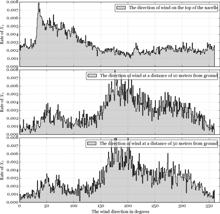
Figure 1: Histogram of wind direction at three levels of height

To read out the data we used the function genfromtxt from numpy L_scipy lib.

⬇

ws1, ws2, ws3 = np.genfromtxt(’data.csv’, delimiter=’;’, skip_header=True, usecols=(2, 4, 6), unpack=True)

where ’data.csv’ is data file, delimiter=’;’ is columns separator, skip_header = True specifies ignoring of the first line as the names of the columns, usecols=(2, 4, 6) makes function to use only 2, 4, 6 columns (numbering begins with zero) and unpack=True — contents of each column should be written in separate arrays ws1, ws2 and ws3 for further analysis of the data separately.

III Probability distributions

Each of distributions is parameterized by three parameters: $\alpha$ — shape factor, $l$ — location factor and $s$ — scale factor. In the case of the beta distribution the second scale factor is added, denoted by $\beta$-letter. All distributions parameters are positive real numbers: $\alpha,\beta,s,l\in\mathbb{R}$, $\alpha,\beta,s>0$, $l\geqslant 0$.

The probability density function (PDF) of a Log-Normal random variable $X$ is:

$$f_{LN}(x;\alpha,l,s)={}\\ {}=\begin{dcases}\frac{1}{(x-l)\alpha\sqrt{2\pi}}\exp\left(-\frac{1}{2}\left(\frac{\ln(x-l)-\ln{s}}{\alpha}\right)^{2}\right),&x\geqslant l.\\ 0,&x<l.\end{dcases}$$ (1)

The probability density function of a Weibull L_Frechet ; L_Weibull random variable $X$ is:

$$f_{W}(x;\alpha,l,s)={}\\ {}=\begin{dcases}\frac{\alpha}{s}\left(\frac{x-l}{s}\right)^{\alpha-1}\exp\left[-\left(\frac{x-l}{s}\right)^{\alpha}\right],&x\geqslant l.\\ 0,&x<l.\end{dcases}$$ (2)

The probability density function of a Gamma random variable $X$ is:

$$f_{\Gamma}(x;\alpha,l,s)=\begin{dcases}\frac{(x-l)^{\alpha-1}\exp\left(-\frac{(x-l)}{s}\right)}{s^{\alpha}\Gamma(\alpha)},&x\geqslant l.\\ 0,&x<l.\end{dcases}$$ (3)

where $\Gamma(\alpha)$ is gamma-function.

The probability density function of a Beta random variable $X$ is:

$$f_{\mathcal{B}}(x;\alpha,\beta,l,s)={}\\ {}=\begin{dcases}\frac{\Gamma(\alpha+\beta)}{s\Gamma(\alpha)\Gamma(\beta)}\left(\dfrac{x-l}{s}\right)^{\alpha-1}\left(1-\frac{x-l}{s}\right)^{\beta-1},&x\geqslant l.\\ 0,&x<l.\end{dcases}$$ (4)

If in PDF formulas of Log-Normal, Weibull and Gamma distributions let $l=0$, and for Beta distribution let $s=1$, we get the formulas of distributions most frequently used in L_Johnson1_en ; L_Nelson .

IV Determination of distributions parameters

In scipy.stats L_scipy following objects are defined: lognorm, weibull_min, gamma and beta. These objects implement distributions we work with. Every one of these objects has PDF function pdf(x, a, [b,] loc, scale) and CDF (cumulative distribution) function cdf(x, a, [b,] loc, scale), where x — function argument, a, b — shape parameters $\alpha$, (and $\beta$ for Beta-distribution), loc and scale are location and scale parameters.

For parameters estimation of our distributions the library scipy.stats provides the function fit(data), which calculates the parameters of distributions by maximum likelihood method and the empirical data. We used this function to calculate parameters of the considered distributions. Then we used pdf and cdf functions to compute values of the probability density function and cumulative distribution function.

There is the example of the code for the case of Log-Normal distribution:

⬇

s, loc, scale = scipy.stats.lognorm.fit(ws1)

xs = np.linspace(np.min(ws1), np.max(ws1), 1000)

logN_PDF = scipy.stats.lognorm.pdf(xs, s, loc, scale)

logN_CDF = scipy.stats.lognorm.cdf(xs, s, loc, scale)

The results are presented graphically on figures 2, 3, 4,  5, 6, 7, 8, 9 and 11, 10, 12, 13. The figures were plotted for theoretical distributions, the parameters of which have been determined on the basis of the entire dataset. From the analysis of the quantile-quantile plots (Q-Q plots) we can conclude that the Weibull distribution is best suited for approximation of available data (although only slightly), outmatching them only in the approximation of extreme values of a random variable.

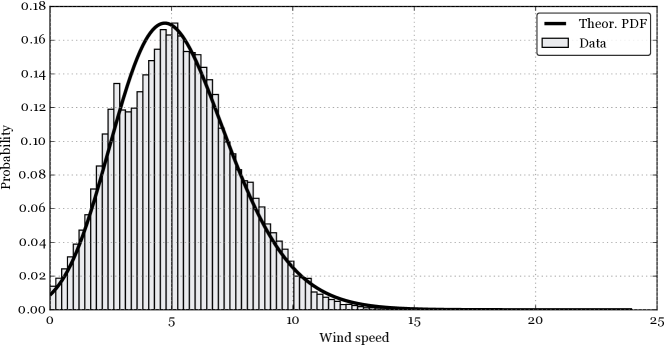
Figure 2: PDF of Log-Normal distribution compared with data histogram

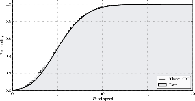
Figure 3: CDF of Log-Normal distribution compared with empirical distribution function

Figure 4: PDF of Weibull distribution compared with data histogram

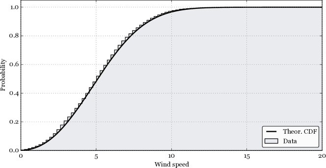
Figure 5: CDF of Weibull distribution compared with empirical distribution function

Figure 6: PDF of Gamma distribution compared with data histogram

Figure 7: CDF of Gamma distribution compared with empirical distribution function

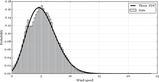
Figure 8: PDF of Beta distribution compared with data histograms

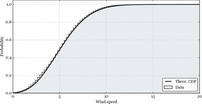
Figure 9: CDF of Beta distribution compared with empirical distribution function

We also performed computations with the considered distributions parameterized by only two parameters (let $l=0$, and for Beta distribution an addition let $s=1$). After plotting the results of calculations we found out that the two-parameter Weibull distribution has superiority over other two-parameters distributions (Log-Normal, Gamma and Beta), which is not true for three-parameter case.

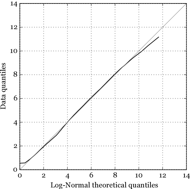
Figure 10: Q-Q plot for LogNormal distribution

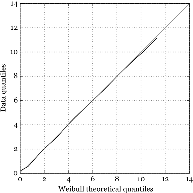
Figure 11: Q-Q plot for Weibull distribution

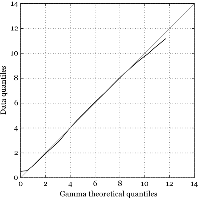
Figure 12: Q-Q plot for Gamma distribution

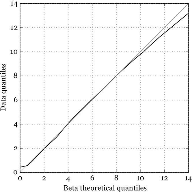
Figure 13: Q-Q plot for Beta distribution

V Conclusions

The results of statistical data processing correspond to the results presented in the literature, where Weibull distribution is the most often used distribution for the wind speed approximation L_Lun2000145 ; L_Seguro200075 ; L_1983WiEng ; L_4488041 ; L_Islam2011985 ; L_Garcia1998139 .

Our future work will be aimed at the construction of stochastic models that can approximate the wind speed depending on time L_1511.02345 . On the other hand, we expect to verify the results of this work by using more dilated and large data array.