Design of Linear Parameter Varying Quadratic Regulator in Polynomial Chaos Framework

Abstract

We present a new theoretical framework for designing linear parameter varying controllers in the polynomial chaos framework. We assume the scheduling variable to be random and apply polynomial chaos approach to synthesize the controller for the resulting linear stochastic dynamical system. Two algorithms are presented that minimize the performance objective with respect to the stochastic system. The first algorithm is based on Galerkin projection and the second algorithm is based on stochastic collocation. LPV controllers from both the algorithms are shown to outperform classical LPV designs with respect to regulator design for nonlinear missile system.

1 Introduction

Linear parameter varying (LPV) systems are of the form

$$\dot{\boldsymbol{x}}=\boldsymbol{A}(\rho)\boldsymbol{x}+\boldsymbol{B}(\rho)\boldsymbol{u},$$ (1)

where system matrices depend on unknown parameter $\rho(t)$, which is measurable in real-time [1, 2]. Many nonlinear systems can be transformed to LPV systems and control systems can be designed using parameter dependent convex optimization problems. Typically, parameter dependent quantities are approximated using a known class of functions such as multilinear basis functions of $\rho$, linear fractional transformations of system matrices, or by gridding the parameter space. Both these approaches result in solution of a finite, but possible large, number of linear matrix inequalities (LMIs). Further, the choice of the basis functions or the resolution of the grid could lead to conservatisms in the design. Clearly, there is a tradeoff between problem size and conservatism in the design [3].

Fujisaki et. al. [4] addressed the computational complexity of such problems by presenting a probabilistic approach to solve these problems, via a sequential randomized algorithm, which significantly reduces the computational complexity. Here the parameter $\rho(t)$ is assumed to be bounded i.e. $\rho(t)\in{\mathcal{D}_{\rho}}\subset{}^{d}$ and is treated as a random variable, with a distribution $f_{\rho}(\rho)$ defined over ${\mathcal{D}_{\rho}}$. The LPV synthesis problem is solved by sampling ${\mathcal{D}_{\rho}}$ and solving the sampled LMIs using a sequential-gradient method. As with any probabilistic algorithm, there is a tradeoff between sample complexity and confidence in the solution. Often, a large number of samples are required to generate a solution with high confidence. Also, the LMIs depend only on $\rho(t)$ and not in $\dot{\rho}(t)$ as it is in classical LPV formulation.

This paper is motivated by the work of Fujisaki et. al.   and is based on the idea of treating $\rho$ as a random variable. Therefore, by substituting $\rho\equiv\boldsymbol{\Delta}$ in the system equation, we get

$$\dot{\boldsymbol{x}} =\boldsymbol{A}(\boldsymbol{\Delta})\boldsymbol{x}+\boldsymbol{B}(\boldsymbol{\Delta})\boldsymbol{u},$$ (2)

where $\boldsymbol{\Delta}\in{}^{d}$ is a vector of uncertain parameters, with joint probability density function $f_{\boldsymbol{\Delta}}(\boldsymbol{\Delta})$. Matrices $\boldsymbol{A}(\boldsymbol{\Delta})\in{}^{n\times n}$, $\boldsymbol{B}(\boldsymbol{\Delta})\in{}^{n\times m}$ are system matrices that depend on $\boldsymbol{\Delta}$. Consequently, the solution $\boldsymbol{x}:=\boldsymbol{x}(t,\boldsymbol{\Delta})\in{}^{n}$ also depends on $\boldsymbol{\Delta}$. Like in [4] we ignore temporal variation in the parameter and thus treat $\boldsymbol{\Delta}$ as random variables. Thus, we now study the system in (1) as a linear time invariant system with probabilistic system parameters. The LPV control design objective is then equivalent to designing a state-feedback law of the form $\boldsymbol{u}=\boldsymbol{K}(\boldsymbol{\Delta})\boldsymbol{x}$, which stabilizes the system in some suitable sense, where $\boldsymbol{K}(\boldsymbol{\Delta})\in{}^{m\times n}$. Thus, we are looking to obtain a parameter dependent gain $\boldsymbol{K}(\boldsymbol{\Delta})$ that stabilizes the system in (2) and optimizes a certain performance index. The closed-loop system is then

$$\dot{\boldsymbol{x}} =\left[\boldsymbol{A}(\boldsymbol{\Delta})+\boldsymbol{B}(\boldsymbol{\Delta})\boldsymbol{K}(\boldsymbol{\Delta})\right]\boldsymbol{x},$$

$$=\boldsymbol{A}_{\textit{cl}}(\boldsymbol{\Delta})\boldsymbol{x}.$$ (3)

There are two distinct differences between the work presented here and that in [4]. We do not use a randomized approach to solve the stochastic problem, and thus don’t have issues related to confidence in the solution. In our approach, the stochastic problem is solved using polynomial chaos theory, which is a deterministic approach as described later. In addition, stability of the LPV system is formulated in an optimal way which minimizes a cost-to-go function for the corresponding stochastic system. In [4], stability of the LPV system is formulated in the probabilistic sense.

Main contribution of this paper is an LPV regulator synthesis algorithm, in the polynomial chaos framework, which generates a parameter dependent gain. The controller is optimal with respect to a quadratic cost in state and control. The paper is organized as follows. We first provide a brief background on polynomial chaos theory and show how it is applied to study linear dynamical systems with random parameters. This is followed by conditions for optimal regulation in the polynomial chaos framework for closed-loop system with parameter dependent controller. This leads to the main controller synthesis related results in the paper. The paper ends with an example nonlinear missile system that highlights the superiority of the polynomial chaos approach over the classical LPV design approach.

2 Polynomial Chaos Theory

Polynomial chaos (PC) is a deterministic method for evolution of uncertainty in dynamical system, when there is probabilistic uncertainty in the system parameters. Polynomial chaos was first introduced by Wiener [5] where Hermite polynomials were used to model stochastic processes with Gaussian random variables. It can be thought of as an extension of Volterra’s theory of nonlinear functionals for stochastic systems [6, 7]. According to Cameron and Martin [8] such an expansion converges in the $\mathcal{L}_{2}$ sense for any arbitrary stochastic process with finite second moment. This applies to most physical systems. Xiu et. al. [9] generalized the result of Cameron-Martin to various continuous and discrete distributions using orthogonal polynomials from the so called Askey-scheme [10] and demonstrated $\mathcal{L}_{2}$ convergence in the corresponding Hilbert functional space. The PC framework has been applied to applications including stochastic fluid dynamics [11, 12, 13], stochastic finite elements [7], and solid mechanics [14, 15], feedback control [16, 17, 18, 19] and estimation [20]. It has been shown that PC based methods are computationally far superior than Monte-Carlo based methods [9, 11, 12, 13, 21]. See [22] for several benchmark problems.

Formally, the PC framework is described as follows. Let $(\Omega,\mathcal{F},P)$ be a probability space, where $\Omega$ is the sample space, $\mathcal{F}$ is the $\sigma$-algebra of the subsets of $\Omega$, and $P$ is the probability measure. Let $\boldsymbol{\Delta}(\omega)=(\boldsymbol{\Delta}_{1}(\omega),\cdots,\boldsymbol{\Delta}_{d}(\omega)):(\Omega,\mathcal{F})\rightarrow(\mathbb{R}^{d},\mathcal{B}^{d})$ be an $\mathbb{R}^{d}$-valued continuous random variable, where $d\in\mathbb{N}$, and $\mathcal{B}^{d}$ is the $\sigma$-algebra of Borel subsets of $\mathbb{R}^{d}$.

A general second order process $X(\omega)\in\mathcal{L}_{2}(\Omega,\mathcal{F},P)$ can be expressed by polynomial chaos as

$$X(\omega)=\sum_{i=0}^{\infty}x_{i}\phi_{i}({\boldsymbol{\Delta}}(\omega)),$$ (4)

where $\omega$ is the random event and $\phi_{i}({\boldsymbol{\Delta}}(\omega))$ denotes the polynomial chaos basis of degree $p$ in terms of the random variables $\boldsymbol{\Delta}(\omega)$. In practice, the infinite series is truncated and $X(\omega)$ is approximated by

$$X(\omega)\approx\hat{X}(\omega)=\sum_{i=0}^{N}x_{i}\phi_{i}({\boldsymbol{\Delta}}(\omega)).$$

The functions $\{\phi_{i}\}$ are a family of orthogonal basis in $\mathcal{L}_{2}(\Omega,\mathcal{F},P)$ satisfying the relation where $\mathcal{D}_{\boldsymbol{\Delta}}$ is the domain of the random variable $\boldsymbol{\Delta}(\omega)$, and $f_{\boldsymbol{\Delta}}(\boldsymbol{\Delta})$ is a probability density function for $\boldsymbol{\Delta}$. Table 1 shows the family of basis functions for random variables with common distributions.

Random Variable $\boldsymbol{\Delta}$	$\phi_{i}(\boldsymbol{\Delta})$ of the Wiener-Askey Scheme
Gaussian	Hermite
Uniform	Legendre
Gamma	Laguerre
Beta	Jacobi

Table 1: Correspondence between choice of polynomials and given distribution of $\boldsymbol{\Delta}(\omega)$ [9].

Generally, there are two methods for expanding a random process in this framework – Galerkin projection and stochastic collocation. These two approaches are described next.

2.1 Galerkin Projection

With respect to the dynamical system defined in (2), the solution can be approximated by the polynomial chaos expansion as

$$\boldsymbol{x}(t,\boldsymbol{\Delta})\approx\hat{\boldsymbol{x}}(t,\boldsymbol{\Delta})=\sum_{i=0}^{N}\boldsymbol{x}_{i}(t)\phi_{i}({\boldsymbol{\Delta}}),$$

where the polynomial chaos coefficients $\boldsymbol{x}_{i}\in{}^{n}$. Define $\boldsymbol{\Phi}(\boldsymbol{\Delta})$ to be

$$\boldsymbol{\Phi} \equiv\boldsymbol{\Phi}(\boldsymbol{\Delta}):=\begin{pmatrix}\phi_{0}({\boldsymbol{\Delta}})&\cdots&\phi_{N}({\boldsymbol{\Delta}})\end{pmatrix}^{T},\text{ and }$$ (10)

$$\boldsymbol{\Phi}_{n} \equiv\boldsymbol{\Phi}_{n}(\boldsymbol{\Delta}):=\boldsymbol{\Phi}(\boldsymbol{\Delta})\otimes\boldsymbol{I}_{{n}},$$ (11)

where $\boldsymbol{I}_{{n}}\in{}^{n\times n}$ is identity matrix. Also define matrix $\boldsymbol{X}\in{}^{n\times(N+1)}$, with polynomial chaos coefficients $\boldsymbol{x}_{i}$, as

$$\boldsymbol{X}=\begin{bmatrix}\boldsymbol{x}_{0}&\cdots&\boldsymbol{x}_{N}\end{bmatrix}.$$

This lets us define $\hat{\boldsymbol{x}}(t,\boldsymbol{\Delta})$ as

$$\hat{\boldsymbol{x}}(t,\boldsymbol{\Delta}):=\boldsymbol{X}(t)\boldsymbol{\Phi}(\boldsymbol{\Delta}).$$ (12)

Noting that $\hat{\boldsymbol{x}}\equiv\boldsymbol{\mathsf{vec}}\left({\hat{\boldsymbol{x}}}\right)$, we obtain an alternate form for (12),

$$\hat{\boldsymbol{x}}\equiv\boldsymbol{\mathsf{vec}}\left({\hat{\boldsymbol{x}}}\right)=\boldsymbol{\mathsf{vec}}\left({\boldsymbol{X}\boldsymbol{\Phi}}\right)=\boldsymbol{\mathsf{vec}}\left({\boldsymbol{I}_{{n}}\boldsymbol{X}\boldsymbol{\Phi}}\right)=(\boldsymbol{\Phi}^{T}\otimes\boldsymbol{I}_{{n}})\boldsymbol{\mathsf{vec}}\left({\boldsymbol{X}}\right)=\boldsymbol{\Phi}_{n}^{T}\boldsymbol{x}_{pc},$$ (13)

where $\boldsymbol{x}_{pc}:=\boldsymbol{\mathsf{vec}}\left({\boldsymbol{X}}\right)$, and $\boldsymbol{\mathsf{vec}}\left({\cdot}\right)$ is the vectorization operator [23].

Since $\hat{\boldsymbol{x}}$ from (13) is an approximation, substituting it in (3) we get equation error $\boldsymbol{e}$, which is given by

$$\boldsymbol{e} :=\dot{\hat{\boldsymbol{x}}}-\boldsymbol{A}_{\textit{cl}}(\boldsymbol{\Delta})\hat{\boldsymbol{x}}=\boldsymbol{\Phi}_{n}^{T}\dot{\boldsymbol{x}}_{pc}-\boldsymbol{A}_{\textit{cl}}(\boldsymbol{\Delta})\boldsymbol{\Phi}_{n}^{T}\boldsymbol{x}_{pc}.$$ (14)

Best $\mathcal{L}_{2}$ approximation is obtained by setting

$$\left\langle\boldsymbol{e}\phi_{i}\right\rangle:=\boldsymbol{\mathsf{E}}\left[\boldsymbol{e}\phi_{i}\right]=0,\text{ for }i=0,1,\cdots,N.$$ (15)

$$\boldsymbol{\mathsf{E}}\left[\boldsymbol{\Phi}_{n}\boldsymbol{\Phi}_{n}^{T}\right]\dot{\boldsymbol{x}}_{pc}=\boldsymbol{\mathsf{E}}\left[\boldsymbol{\Phi}_{n}\boldsymbol{A}_{\textit{cl}}\boldsymbol{\Phi}_{n}^{T}\right]\boldsymbol{x}_{pc},$$

$$\implies\dot{\boldsymbol{x}}_{pc}=\boldsymbol{\mathsf{E}}\left[\boldsymbol{\Phi}_{n}\boldsymbol{\Phi}_{n}^{T}\right]^{-1}\boldsymbol{\mathsf{E}}\left[\boldsymbol{\Phi}_{n}\boldsymbol{A}_{\textit{cl}}\boldsymbol{\Phi}_{n}^{T}\right]\boldsymbol{x}_{pc},$$ (16)

$$\text{or }\dot{\boldsymbol{x}}_{pc}=\boldsymbol{A}_{pc}\boldsymbol{x}_{pc}.$$ (17)

where $\boldsymbol{\Phi}_{n}$ and $\boldsymbol{A}_{\textit{cl}}$ depend on $\boldsymbol{\Delta}$ as defined earlier. Equation (17), is best finite dimensional approximation of (3) in the $\mathcal{L}_{2}$ sense.

2.2 Stochastic Collocation

In this approach, we introduce Lagrangian interpolants

$$l_{i}(\boldsymbol{\Delta})=\prod^{N}_{j=0,j\neq i}\frac{\boldsymbol{\Delta}-\boldsymbol{\Delta}_{j}}{\boldsymbol{\Delta}_{i}-\boldsymbol{\Delta}_{j}}$$

as basis functions, where $\boldsymbol{\Delta}_{i}$ are the roots of the polynomial chaos basis of degree $N+1$. The Lagrange interpolants are orthogonal to each other in the $\mathcal{L}_{2}$ sense, which can be proved using Gaussian quadrature rule as follows.

$$\boldsymbol{\mathsf{E}}\left[l_{i}l_{j}\right] =\int_{\mathcal{D}_{\boldsymbol{\Delta}}}l_{i}(\boldsymbol{\Delta})l_{j}(\boldsymbol{\Delta})f_{\boldsymbol{\Delta}}(\boldsymbol{\Delta})d\boldsymbol{\Delta}$$

$$=\sum_{k=0}^{N}\int_{\mathcal{D}_{\boldsymbol{\Delta}}}l_{k}(\boldsymbol{\Delta})f_{\boldsymbol{\Delta}}(\boldsymbol{\Delta})d\boldsymbol{\Delta}l_{i}(\boldsymbol{\Delta}_{k})l_{j}(\boldsymbol{\Delta}_{k}).$$

Since $i\neq j$, we can conclude

$$\boldsymbol{\mathsf{E}}\left[l_{i}l_{j}\right]=0.$$

The solution to the dynamical system (3) thus can also be approximated as

$$\boldsymbol{x}(t,\boldsymbol{\Delta})\approx\tilde{\boldsymbol{x}}=\sum_{i=0}^{N}\boldsymbol{x}_{i,sc}(t)l_{i}(\boldsymbol{\Delta})=\boldsymbol{L}_{n}^{T}\boldsymbol{x}_{sc},$$

where $\boldsymbol{L}_{n}=\left[l_{0}\ldots l_{N}\right]^{T}\otimes\boldsymbol{I}_{{n}}$, and $\boldsymbol{x}_{sc}=[\boldsymbol{x}_{0,sc}\ldots\boldsymbol{x}_{N,sc}]^{T}$ are coefficients determined by solving $\dot{\boldsymbol{x}}_{i,sc}=\boldsymbol{A}_{cl}(\boldsymbol{\Delta}_{i})\boldsymbol{x}_{i,sc}$. It implies that the solution $\tilde{\boldsymbol{x}}$ is exact at those specified sample points, which means that the error $\tilde{\boldsymbol{e}}=\dot{\tilde{\boldsymbol{x}}}-\boldsymbol{A}_{cl}(\boldsymbol{\Delta})\tilde{\boldsymbol{x}}$ is forced to be zero at the sample points $\boldsymbol{\Delta}_{i}$.

We need the following result to derive the optimal control law in the stochastic collocation setting.

Lemma 1.

Consider two Lagrangian interpolants $l_{i}(\boldsymbol{\Delta})$ and $l_{j}(\boldsymbol{\Delta})$ , and a function $g(\boldsymbol{\Delta})$, then

$$\boldsymbol{\mathsf{E}}\left[l_{i}(\boldsymbol{\Delta})l_{j}(\boldsymbol{\Delta})g(\boldsymbol{\Delta})\right]=\begin{cases}0,&i\neq j\\ \boldsymbol{\mathsf{E}}\left[l_{i}(\boldsymbol{\Delta})\right]g(\boldsymbol{\Delta}_{i}),&i=j\end{cases},$$ (18)

if $g(\boldsymbol{\Delta})$ is affine in $\boldsymbol{\Delta}$.

Proof.

$$\boldsymbol{\mathsf{E}}\left[l_{i}(\boldsymbol{\Delta})l_{j}(\boldsymbol{\Delta})g(\boldsymbol{\Delta})\right]=\int_{\mathcal{D}_{\boldsymbol{\Delta}}}l_{i}(\boldsymbol{\Delta})l_{j}(\boldsymbol{\Delta})g(\boldsymbol{\Delta})f_{\boldsymbol{\Delta}}(\boldsymbol{\Delta})d\boldsymbol{\Delta}$$

$$\approx\sum_{m=0}^{N}\int_{\mathcal{D}_{\boldsymbol{\Delta}}}l_{m}(\boldsymbol{\Delta})f_{\boldsymbol{\Delta}}(\boldsymbol{\Delta})d\boldsymbol{\Delta}l_{i}(\boldsymbol{\Delta}_{m})l_{j}(\boldsymbol{\Delta}_{m})g(\boldsymbol{\Delta}_{m})$$

$$=\begin{cases}0&i\neq j\\ \int_{\mathcal{D}_{\boldsymbol{\Delta}}}l_{i}(\boldsymbol{\Delta})f_{\boldsymbol{\Delta}}(\boldsymbol{\Delta})d\boldsymbol{\Delta}g(\boldsymbol{\Delta}_{i})&i=j\end{cases}$$

$$=\begin{cases}0&i\neq j\\ \boldsymbol{\mathsf{E}}\left[l_{i}(\boldsymbol{\Delta})\right]g(\boldsymbol{\Delta}_{i})&i=j\end{cases},$$

According to Gaussian quadrature rule, the expression is exact when $l_{i}l_{j}g$ is a polynomial of degree at most $2N+1$. It is known that the Lagrangian interpolants are N-th order polynomials, so we can conclude that if $g$ is affine in $\boldsymbol{\Delta}$, (18) is exact. ∎

We next present synthesis of optimal control law using both Galerkin projection and stochastic collocation approach.

3 Optimal Controller Synthesis

Given the system in (2) we are interested in state feedback control $\boldsymbol{u}:=\boldsymbol{K}(\boldsymbol{\Delta})\boldsymbol{x}(t,\boldsymbol{\Delta})$ that minimizes the following cost function

$$\min_{\boldsymbol{u}}\boldsymbol{\mathsf{E}}\left[\int_{0}^{\infty}(\boldsymbol{x}^{T}\boldsymbol{Q}\boldsymbol{x}+\boldsymbol{u}^{T}\boldsymbol{R}\boldsymbol{u})\,dt\right].$$ (19)

If $\exists$ $V(\boldsymbol{x})>0$ such that

$$\boldsymbol{\mathsf{E}}\left[\frac{dV}{dt}\right]\leq-\boldsymbol{\mathsf{E}}\left[\boldsymbol{x}^{T}\boldsymbol{Q}\boldsymbol{x}+\boldsymbol{u}^{T}\boldsymbol{R}\boldsymbol{u}\right].$$ (20)

Integrating from $[0,T]$ gives us

$$\int_{0}^{T}\boldsymbol{\mathsf{E}}\left[\frac{dV}{dt}\right]dt \leq-\int_{0}^{T}\boldsymbol{\mathsf{E}}\left[\boldsymbol{x}^{T}\boldsymbol{Q}\boldsymbol{x}+\boldsymbol{u}^{T}\boldsymbol{R}\boldsymbol{u}\right]dt,$$

$$\boldsymbol{\mathsf{E}}\left[V(\boldsymbol{x}(T))\right]-\boldsymbol{\mathsf{E}}\left[V(\boldsymbol{x}(0))\right] \leq-\int_{0}^{T}\boldsymbol{\mathsf{E}}\left[\boldsymbol{x}^{T}\boldsymbol{Q}\boldsymbol{x}+\boldsymbol{u}^{T}\boldsymbol{R}\boldsymbol{u}\right]dt,$$

since $\boldsymbol{\mathsf{E}}\left[V(\boldsymbol{x}(T))\right]\geq 0$ implies

$$-\boldsymbol{\mathsf{E}}\left[V(\boldsymbol{x}(0))\right]\leq-\int_{0}^{T}\boldsymbol{\mathsf{E}}\left[\boldsymbol{x}^{T}\boldsymbol{Q}\boldsymbol{x}+\boldsymbol{u}^{T}\boldsymbol{R}\boldsymbol{u}\right]dt,\text{ for all $T>0$},$$ (21)

or,

$$\boldsymbol{\mathsf{E}}\left[V(\boldsymbol{x}(0))\right]\geq\int_{0}^{\infty}\boldsymbol{\mathsf{E}}\left[\boldsymbol{x}^{T}\boldsymbol{Q}\boldsymbol{x}+\boldsymbol{u}^{T}\boldsymbol{R}\boldsymbol{u}\right]dt.$$ (22)

Therefore, (20) provides a sufficient condition for upper bound on the cost-to-go.

In this paper, we use polynomial chaos theory to determine the expectation operator in (20). We apply both Galerkin projection and stochastic collocation techniques, and derive control synthesis problem in the respective frameworks, for the system considered in (2). We will see later, the Galerkin projection is more accurate than stochastic collocation technique, but results in more complex synthesis problems. Consequently, the computational time for synthesis is more, but generates better performing controller.

Before we proceed, we need the following result in the rest of the paper.

Proposition 1.

For any vector $\boldsymbol{v}\in{}^{N+1}$ and matrix $\boldsymbol{M}\in{}^{m\times n}$

$$\boldsymbol{M}(\boldsymbol{v}^{T}\otimes\boldsymbol{I}_{{n}})=(\boldsymbol{v}^{T}\otimes\boldsymbol{I}_{{m}})(\boldsymbol{I}_{{N+1}}\otimes\boldsymbol{M}),$$ (23)

where $\boldsymbol{I}_{{\ast}}$ is identity matrix with indicated dimension.

Proof.

$$\boldsymbol{M}(\boldsymbol{v}^{T}\otimes\boldsymbol{I}_{{n}}) =(1\otimes\boldsymbol{M})(\boldsymbol{v}^{T}\otimes\boldsymbol{I}_{{n}})$$

$$=\boldsymbol{v}^{T}\otimes\boldsymbol{M}=(\boldsymbol{v}^{T}\boldsymbol{I}_{{N+1}})\otimes(\boldsymbol{I}_{{m}}\boldsymbol{M})$$

$$=(\boldsymbol{v}^{T}\otimes\boldsymbol{I}_{{m}})(\boldsymbol{I}_{{N+1}}\otimes\boldsymbol{M}).$$

∎

3.1 Galerkin Projection Based Formulation

Here Galerkin projection is used to solve the stochastic optimal control problem. Using the parameterization given by (13), and the sufficient condition in (20), we present the following optimal control law synthesis algorithm.

Theorem 2.

Controller gain $\boldsymbol{K}(\boldsymbol{\Delta}):=\boldsymbol{W}(\boldsymbol{\Delta})\boldsymbol{Y}^{-1}(\boldsymbol{\Delta})$ minimizes (19) if $\exists$ $\boldsymbol{Y}(\boldsymbol{\Delta})=\boldsymbol{Y}^{T}(\boldsymbol{\Delta})>0\in{}^{n\times n}$ and $\boldsymbol{W}(\boldsymbol{\Delta})=\boldsymbol{W}^{T}(\boldsymbol{\Delta})>0\in{}^{m\times n}$, which are the solutions of the optimization problem

$$\max\mathbf{tr\;}\boldsymbol{\mathsf{E}}\left[\boldsymbol{Y}(\boldsymbol{\Delta})\right]$$ (24)

subject to

$$\boldsymbol{\mathsf{E}}\left[\mathsf{sym}\left(\mathcal{Y}\boldsymbol{\Phi}_{n}\boldsymbol{A}^{T}\boldsymbol{\Phi}_{n}^{T}+\mathcal{W}^{T}\boldsymbol{\Phi}_{m}\boldsymbol{B}^{T}\boldsymbol{\Phi}_{n}\right)+\mathcal{Y}\boldsymbol{\Phi}_{n}\boldsymbol{Q}\boldsymbol{\Phi}_{n}^{T}\mathcal{Y}\right]+\boldsymbol{\mathsf{E}}\left[\mathcal{W}^{T}\boldsymbol{\Phi}_{m}\boldsymbol{R}\boldsymbol{\Phi}_{m}^{T}\mathcal{W}\right]\leq 0,$$ (25)

where $\mathcal{Y}:=\boldsymbol{I}_{{N+1}}\otimes\boldsymbol{Y}(\boldsymbol{\Delta})$ and $\mathcal{W}:=\boldsymbol{I}_{{N+1}}\otimes\boldsymbol{W}(\boldsymbol{\Delta})$, and $\mathsf{sym}\left(\boldsymbol{X}\right):=\boldsymbol{X}+\boldsymbol{X}^{T}$.

Proof.

Let $V(\boldsymbol{x}):=\boldsymbol{x}^{T}\boldsymbol{P}(\boldsymbol{\Delta})\boldsymbol{x},\boldsymbol{P}(\boldsymbol{\Delta})=\boldsymbol{P}^{T}(\boldsymbol{\Delta})>0\in{}^{n\times n}$. Therefore, (20) can be written as

$$\boldsymbol{\mathsf{E}}\left[\boldsymbol{x}^{T}\left(\mathsf{sym}\left((\boldsymbol{A}+\boldsymbol{B}\boldsymbol{K})^{T}\boldsymbol{P}\right)+\boldsymbol{Q}+\boldsymbol{K}^{T}\boldsymbol{R}\boldsymbol{K}\right)\boldsymbol{x}\right]\leq 0,$$

or

$$\boldsymbol{\mathsf{E}}\left[\boldsymbol{x}^{T}\left(\mathsf{sym}\left(\boldsymbol{A}^{T}\boldsymbol{P}+\boldsymbol{K}^{T}\boldsymbol{B}^{T}\boldsymbol{P}\right)+\boldsymbol{Q}+\boldsymbol{K}^{T}\boldsymbol{R}\boldsymbol{K}\right)\boldsymbol{x}\right]\leq 0.$$ (26)

Substituting $\boldsymbol{P}:=\boldsymbol{Y}^{-1}$ and $\boldsymbol{x}:=\boldsymbol{Y}\boldsymbol{z}$, in the above quadratic form, we get

$$\boldsymbol{x}^{T}\left(\mathsf{sym}\left(\boldsymbol{P}\boldsymbol{A}+\boldsymbol{P}\boldsymbol{B}\boldsymbol{K}\right)+\boldsymbol{Q}+\boldsymbol{K}^{T}\boldsymbol{R}\boldsymbol{K}\right)\boldsymbol{x}$$

$$=\boldsymbol{z}^{T}\boldsymbol{Y}\left(\mathsf{sym}\left(\boldsymbol{Y}^{-1}\boldsymbol{A}+\boldsymbol{Y}^{-1}\boldsymbol{B}\boldsymbol{K}\right)+\boldsymbol{Q}+\boldsymbol{K}^{T}\boldsymbol{R}\boldsymbol{K}\right)\boldsymbol{Y}\boldsymbol{z}$$

$$=\boldsymbol{z}^{T}\left(\mathsf{sym}\left(\boldsymbol{A}\boldsymbol{Y}+\boldsymbol{B}\boldsymbol{K}\boldsymbol{Y}\right)+\boldsymbol{Y}\boldsymbol{Q}\boldsymbol{Y}+\boldsymbol{Y}\boldsymbol{K}^{T}\boldsymbol{R}\boldsymbol{K}\boldsymbol{Y}\right)\boldsymbol{z}$$

With $\boldsymbol{W}:=\boldsymbol{K}\boldsymbol{Y}$, the quadratic form simplifies to

$$\boldsymbol{z}^{T}\left(\mathsf{sym}\left(\boldsymbol{A}\boldsymbol{Y}+\boldsymbol{B}\boldsymbol{W}\right)+\boldsymbol{Y}\boldsymbol{Q}\boldsymbol{Y}+\boldsymbol{W}^{T}\boldsymbol{R}\boldsymbol{W}\right)\boldsymbol{z}.$$

Therefore, the condition in (26) is equivalent to

$$\boldsymbol{\mathsf{E}}\left[\boldsymbol{z}^{T}\left(\mathsf{sym}(\boldsymbol{A}\boldsymbol{Y}+\boldsymbol{B}\boldsymbol{W})+\boldsymbol{Y}\boldsymbol{Q}\boldsymbol{Y}+\boldsymbol{W}^{T}\boldsymbol{R}\boldsymbol{W}\right)\boldsymbol{z}\right]\leq 0.$$ (27)

Assuming, $\boldsymbol{z}(t,\boldsymbol{\Delta})$ is a second order process, we can represent

$$\boldsymbol{z}(t,\boldsymbol{\Delta}):=\sum_{i=0}^{\infty}\boldsymbol{x}_{i}(t)\phi_{i}({\boldsymbol{\Delta}})=\boldsymbol{\Phi}_{n}^{T}(\boldsymbol{\Delta})\boldsymbol{z}_{pc}(t).$$

Note that we have included infinite terms in the polynomial expansion, and thus the representation is exact.

With $\boldsymbol{z}=\boldsymbol{\Phi}_{n}^{T}\boldsymbol{z}_{pc}$, we get

$$\boldsymbol{z}_{pc}^{T}\boldsymbol{\mathsf{E}}\left[\mathsf{sym}\left(\boldsymbol{\Phi}_{n}\boldsymbol{Y}\boldsymbol{A}^{T}\boldsymbol{\Phi}_{n}^{T}+\boldsymbol{\Phi}_{n}\boldsymbol{W}^{T}\boldsymbol{B}^{T}\boldsymbol{\Phi}_{n}^{T}\right)+\boldsymbol{\Phi}_{n}\boldsymbol{Y}\boldsymbol{Q}\boldsymbol{Y}\boldsymbol{\Phi}_{n}^{T}+\boldsymbol{\Phi}_{n}\boldsymbol{W}^{T}\boldsymbol{R}\boldsymbol{W}\boldsymbol{\Phi}_{n}^{T}\right]\boldsymbol{z}_{pc}\leq 0,$$

or

$$\boldsymbol{\mathsf{E}}\left[\mathsf{sym}\left(\boldsymbol{\Phi}_{n}\boldsymbol{Y}\boldsymbol{A}^{T}\boldsymbol{\Phi}_{n}^{T}+\boldsymbol{\Phi}_{n}\boldsymbol{W}^{T}\boldsymbol{B}^{T}\boldsymbol{\Phi}_{n}^{T}\right)+\boldsymbol{\Phi}_{n}\boldsymbol{Y}\boldsymbol{Q}\boldsymbol{Y}\boldsymbol{\Phi}_{n}^{T}+\boldsymbol{\Phi}_{n}\boldsymbol{W}^{T}\boldsymbol{R}\boldsymbol{W}\boldsymbol{\Phi}_{n}^{T}\right]\leq 0.$$

Using (23) we can write $\boldsymbol{\Phi}_{n}\boldsymbol{Y}=\mathcal{Y}\boldsymbol{\Phi}_{n}$ and $\boldsymbol{\Phi}_{n}\boldsymbol{W}^{T}=\mathcal{W}^{T}\boldsymbol{\Phi}_{m}$. Substituting them, we get

$$\boldsymbol{\mathsf{E}}\left[\mathsf{sym}\left(\mathcal{Y}\boldsymbol{\Phi}_{n}\boldsymbol{A}^{T}\boldsymbol{\Phi}_{n}^{T}+\mathcal{W}^{T}\boldsymbol{\Phi}_{m}\boldsymbol{B}^{T}\boldsymbol{\Phi}_{n}\right)+\mathcal{Y}\boldsymbol{\Phi}_{n}\boldsymbol{Q}\boldsymbol{\Phi}_{n}^{T}\mathcal{Y}+\mathcal{W}^{T}\boldsymbol{\Phi}_{m}\boldsymbol{R}\boldsymbol{\Phi}_{m}^{T}\mathcal{W}\right]\leq 0.$$

Since $\boldsymbol{x}_{0}$ is given, with no initial condition uncertainty, the cost function can be written as

$$\boldsymbol{\mathsf{E}}\left[\boldsymbol{x}_{0}^{T}\boldsymbol{P}(\boldsymbol{\Delta})\boldsymbol{x}_{0}\right]=\boldsymbol{x}_{0}^{T}\boldsymbol{\mathsf{E}}\left[\boldsymbol{P}(\boldsymbol{\Delta})\right]\boldsymbol{x}_{0}=\boldsymbol{x}_{0}^{T}\boldsymbol{\mathsf{E}}\left[\boldsymbol{Y}^{-1}(\boldsymbol{\Delta})\right]\boldsymbol{x}_{0}.$$

Therefore for a given $\boldsymbol{x}_{0}$,

$$\max\mathbf{tr\;}\boldsymbol{\mathsf{E}}\left[\boldsymbol{Y}(\boldsymbol{\Delta})\right] \implies\min\mathbf{tr\;}\boldsymbol{\mathsf{E}}\left[\boldsymbol{P}(\boldsymbol{\Delta})\right]$$

$$\implies\min\boldsymbol{x}_{0}^{T}\boldsymbol{\mathsf{E}}\left[\boldsymbol{P}(\boldsymbol{\Delta})\right]\boldsymbol{x}_{0}$$

∎

The matrix variables $\boldsymbol{Y}(\boldsymbol{\Delta})$ and $\boldsymbol{W}(\boldsymbol{\Delta})$ in (25) are infinite dimensional. In this paper, we consider finite dimensional parameterization of $\boldsymbol{Y}(\boldsymbol{\Delta})=\boldsymbol{Y}(\boldsymbol{\Delta})^{T}>0$ from the literature on sum-of-square (SOS) representation of matrix polynomials [24], defined by the following.

Lemma 3.

(Lemma 1 in [24]) The polynomial matrix $\boldsymbol{Y}(\boldsymbol{\Delta})$ of dimension $n\times n$ is SOS with respect to the monomial basis $\boldsymbol{\Phi}(\boldsymbol{\Delta})$ iff there exists a symmetric matrix $\bar{\boldsymbol{Y}}$ such that

$$\boldsymbol{Y}(\boldsymbol{\Delta})=\left(\boldsymbol{\Phi}(\boldsymbol{\Delta})\otimes\boldsymbol{I}_{{n}}\right)^{T}\bar{\boldsymbol{Y}}\left(\boldsymbol{\Phi}(\boldsymbol{\Delta})\otimes\boldsymbol{I}_{{n}}\right)=\boldsymbol{\Phi}_{n}^{T}(\boldsymbol{\Delta})\bar{\boldsymbol{Y}}\boldsymbol{\Phi}_{n}(\boldsymbol{\Delta}),\text{ and }\bar{\boldsymbol{Y}}\in{}^{n(N+1)\times n(N+1)}\geq 0.$$ (28)

Proof.

See Lemma 1 in [24]. ∎

Therefore, $\boldsymbol{Y}(\boldsymbol{\Delta})=\boldsymbol{Y}(\boldsymbol{\Delta})^{T}>0,\;\forall\boldsymbol{\Delta}\;\Leftrightarrow\;\bar{\boldsymbol{Y}}=\bar{\boldsymbol{Y}}^{T}>0$.

Corollary 1.

$\bar{\boldsymbol{Y}}$ in (28) admits a linear space of $n(n+1)(N+1)(N+2)/4$.

Proof.

Partition $\bar{\boldsymbol{Y}}$ as

$$\bar{\boldsymbol{Y}}:=\begin{bmatrix}\bar{\boldsymbol{Y}}_{00}&\cdots&\bar{\boldsymbol{Y}}_{0N}\\ \vdots&&\vdots\\ \bar{\boldsymbol{Y}}_{N0}&\cdots&\bar{\boldsymbol{Y}}_{NN}\\ \end{bmatrix},$$ (29)

where $\bar{\boldsymbol{Y}}_{ij}=\bar{\boldsymbol{Y}}_{ji}^{T}\in{}^{n\times n}$. Therefore,

$$\boldsymbol{Y}(\boldsymbol{\Delta}) :=\boldsymbol{\Phi}_{n}^{T}\bar{\boldsymbol{Y}}\boldsymbol{\Phi}_{n}=\sum_{ij}\phi_{i}(\boldsymbol{\Delta})\phi_{j}(\boldsymbol{\Delta})\bar{\boldsymbol{Y}}_{ij}.$$ (30)

But, $\boldsymbol{Y}(\boldsymbol{\Delta})=\boldsymbol{Y}(\boldsymbol{\Delta})^{T}$

$$\implies\bar{\boldsymbol{Y}}_{ij}=\bar{\boldsymbol{Y}}_{ij}^{T}.$$ (31)

Combining (29) and (31) we observe that $\bar{\boldsymbol{Y}}$ admits a linear space of dimension $n(n+1)(N+1)(N+2)/4$. ∎

Matrix variable $\boldsymbol{W}(\boldsymbol{\Delta})$ is parameterized to be linearly dependent on polynomial chaos basis functions $\phi_{i}(\boldsymbol{\Delta})$, i.e.

$$\boldsymbol{W}(\boldsymbol{\Delta})=\sum_{i=0}^{N}\boldsymbol{W}_{i}\phi_{i}(\boldsymbol{\Delta}).$$ (32)

From (30), we can write

$$\boldsymbol{Y}(\boldsymbol{\Delta}) =\sum_{ij}\phi_{i}(\boldsymbol{\Delta})\phi_{j}(\boldsymbol{\Delta})\bar{\boldsymbol{Y}}_{ij},$$ (33)

$$=\left(\boldsymbol{\psi}^{T}(\boldsymbol{\Delta})\otimes\boldsymbol{I}_{{n}}\right)\boldsymbol{V}_{\bar{\boldsymbol{Y}}}=\boldsymbol{\psi}^{T}_{n}(\boldsymbol{\Delta})\boldsymbol{V}_{\bar{\boldsymbol{Y}}},$$ (34)

where $\boldsymbol{\psi}^{T}_{n}(\boldsymbol{\Delta}):=\boldsymbol{\psi}^{T}(\boldsymbol{\Delta})\otimes\boldsymbol{I}_{{n}}$,

$$\boldsymbol{\psi}(\boldsymbol{\Delta}):=\begin{bmatrix}\phi_{0}^{2}(\boldsymbol{\Delta})\\ 2\phi_{1}(\boldsymbol{\Delta})\phi_{0}(\boldsymbol{\Delta})\\ \vdots\\ 2\phi_{N}(\boldsymbol{\Delta})\phi_{N-1}(\boldsymbol{\Delta})\\ \phi_{N}^{2}(\boldsymbol{\Delta})\end{bmatrix}$$

and

$$\boldsymbol{V}_{\bar{\boldsymbol{Y}}}:=\begin{pmatrix}\bar{\boldsymbol{Y}}_{00}\\ \bar{\boldsymbol{Y}}_{10}\\ \vdots\\ \bar{\boldsymbol{Y}}_{N(N-1)}\\ \bar{\boldsymbol{Y}}_{NN}\end{pmatrix}$$ (35)

Matrix variable $\boldsymbol{W}(\boldsymbol{\Delta})$ can be written in similar form,

$$\boldsymbol{W}(\boldsymbol{\Delta}) =\sum_{i=0}^{N}\boldsymbol{W}_{i}\phi_{i}(\boldsymbol{\Delta})=\begin{bmatrix}\phi_{0}(\boldsymbol{\Delta})\boldsymbol{I}_{{m}}&\cdots&\phi_{N}(\boldsymbol{\Delta})\boldsymbol{I}_{{m}}\end{bmatrix}\underbrace{\begin{pmatrix}\boldsymbol{W}_{0}\\ \vdots\\ \boldsymbol{W}_{N}\end{pmatrix}}_{\boldsymbol{V}_{\boldsymbol{W}}}=\boldsymbol{\Phi}_{m}^{T}(\boldsymbol{\Delta})\boldsymbol{V}_{\boldsymbol{W}}.$$ (36)

From the definition of $\mathcal{Y}$

$$\mathcal{Y} :=\boldsymbol{I}_{{N+1}}\otimes\boldsymbol{Y}(\boldsymbol{\Delta})=\boldsymbol{I}_{{N+1}}\otimes\Big{(}\boldsymbol{\psi}^{T}_{n}(\boldsymbol{\Delta})\boldsymbol{V}_{\bar{\boldsymbol{Y}}}\Big{)}=\Big{(}\boldsymbol{I}_{{N+1}}\otimes\ \boldsymbol{\psi}^{T}_{n}(\boldsymbol{\Delta})\Big{)}(\boldsymbol{I}_{{N+1}}\otimes\boldsymbol{V}_{\bar{\boldsymbol{Y}}}),$$

$$=\Big{(}\boldsymbol{I}_{{N+1}}\otimes\ \boldsymbol{\psi}^{T}_{n}(\boldsymbol{\Delta})\Big{)}\mathcal{V}_{\bar{\boldsymbol{Y}}}.$$ (37)

Similarly,

$$\mathcal{W} =\boldsymbol{I}_{{N+1}}\otimes\left(\boldsymbol{\Phi}_{m}^{T}(\boldsymbol{\Delta})\boldsymbol{V}_{\boldsymbol{W}}\right)=\Big{(}\boldsymbol{I}_{{N+1}}\otimes\boldsymbol{\Phi}_{m}^{T}(\boldsymbol{\Delta})\Big{)}\mathcal{V}_{\boldsymbol{W}}.$$ (38)

We next present the synthesis algorithm for the particular parameterization considered here.

Theorem 4.

Controller gain

$$\boldsymbol{K}(\boldsymbol{\Delta})=\left(\sum_{i=0}^{N}\boldsymbol{W}_{i}\phi_{i}(\boldsymbol{\Delta})\right)\left(\boldsymbol{\Phi}_{n}^{T}(\boldsymbol{\Delta})\bar{\boldsymbol{Y}}\boldsymbol{\Phi}_{n}(\boldsymbol{\Delta})\right)^{-1},$$

minimizes (19) if matrices $\bar{\boldsymbol{Y}}=\bar{\boldsymbol{Y}}^{T}>0\in{}^{n(N+1)\times n(N+1)}$ and $\boldsymbol{W}_{i}\in{}^{m\times n}$, are the solution of the following optimization problem

$$\max_{\bar{\boldsymbol{Y}},\boldsymbol{W}_{i}}\mathbf{tr\;}\left(\sum_{i=0}^{N}\boldsymbol{\mathsf{E}}\left[\phi_{i}^{2}(\boldsymbol{\Delta})\right]\bar{\boldsymbol{Y}}_{ii}\right)$$

subject to (39)

$$\begin{bmatrix}\mathsf{sym}\left(\mathcal{V}_{\bar{\boldsymbol{Y}}}^{T}\boldsymbol{M}_{1}+\mathcal{V}_{\boldsymbol{W}}^{T}\boldsymbol{M}_{2}\right)&\mathcal{V}_{\bar{\boldsymbol{Y}}}^{T}\sqrt{\boldsymbol{M}_{3}}&\mathcal{V}_{\boldsymbol{W}}^{T}\sqrt{\boldsymbol{M}_{4}}\\[2.84526pt] \sqrt{\boldsymbol{M}_{3}}\mathcal{V}_{\bar{\boldsymbol{Y}}}&-\boldsymbol{I}&\boldsymbol{0}\\[2.84526pt] \sqrt{\boldsymbol{M}_{4}}\mathcal{V}_{\boldsymbol{W}}&\boldsymbol{0}&-\boldsymbol{I}\end{bmatrix}\leq 0,$$ (40)

where $\mathcal{V}_{\bar{\boldsymbol{Y}}}:=\boldsymbol{I}_{{N+1}}\otimes\boldsymbol{V}_{\bar{\boldsymbol{Y}}},\mathcal{V}_{\boldsymbol{W}}:=\boldsymbol{I}_{{N+1}}\otimes\boldsymbol{V}_{\boldsymbol{W}}$, $\boldsymbol{V}_{\bar{\boldsymbol{Y}}},\boldsymbol{V}_{\boldsymbol{W}}$ are functions of $\bar{\boldsymbol{Y}}$ and $\boldsymbol{W}_{i}$ defined in (35) and (36) respectively,

$$\boldsymbol{M}_{1} :=\boldsymbol{\mathsf{E}}\left[(\boldsymbol{I}_{{N+1}}\otimes\boldsymbol{\psi}_{n})\boldsymbol{\Phi}_{n}\boldsymbol{A}^{T}\boldsymbol{\Phi}_{n}^{T}\right],$$ (41)

$$\boldsymbol{M}_{2} :=\boldsymbol{\mathsf{E}}\left[(\boldsymbol{I}_{{N+1}}\otimes\boldsymbol{\Phi}_{m})\boldsymbol{\Phi}_{m}\boldsymbol{B}^{T}\boldsymbol{\Phi}_{n}^{T}\right],$$ (42)

$$\boldsymbol{M}_{3} :=\boldsymbol{\mathsf{E}}\left[(\boldsymbol{I}_{{N+1}}\otimes\boldsymbol{\psi}_{n})\boldsymbol{\Phi}_{n}\boldsymbol{Q}\boldsymbol{\Phi}_{n}^{T}(\boldsymbol{I}_{{N+1}}\otimes\boldsymbol{\psi}^{T}_{n})\right],$$ (43)

$$\boldsymbol{M}_{4} :=\boldsymbol{\mathsf{E}}\left[(\boldsymbol{I}_{{N+1}}\otimes\boldsymbol{\Phi}_{m})\boldsymbol{\Phi}_{m}\boldsymbol{R}\boldsymbol{\Phi}_{m}^{T}(\boldsymbol{I}_{{N+1}}\otimes\boldsymbol{\Phi}_{m}^{T})\right],$$ (44)

and $\sqrt{\boldsymbol{M}_{3}},\sqrt{\boldsymbol{M}_{4}}$ are the principal square roots of the respective matrices.

Proof.

Recall from (33), $\boldsymbol{Y}(\boldsymbol{\Delta})=\sum_{ij}\phi_{i}(\boldsymbol{\Delta})\phi_{j}(\boldsymbol{\Delta})\bar{\boldsymbol{Y}}_{ij}$. Noting that $\boldsymbol{\mathsf{E}}\left[\phi_{i}(\boldsymbol{\Delta})\phi_{j}(\boldsymbol{\Delta})\right]=0$, for $i\neq j$, the cost function in (24) is then

$$\mathbf{tr\;}\boldsymbol{\mathsf{E}}\left[\boldsymbol{Y}(\boldsymbol{\Delta})\right]=\mathbf{tr\;}\Big{(}\sum_{i=0}^{N}\boldsymbol{\mathsf{E}}\left[\phi_{i}^{2}(\boldsymbol{\Delta})\right]\bar{\boldsymbol{Y}}_{ii}\Big{)}.$$ (45)

From (37) and (38), we can substitute $\mathcal{Y}$ and $\mathcal{W}$ in (25) to get

$$\mathsf{sym}\left(\mathcal{V}_{\bar{\boldsymbol{Y}}}^{T}\boldsymbol{\mathsf{E}}\left[(\boldsymbol{I}_{{N+1}}\otimes\boldsymbol{\psi}_{n})\boldsymbol{\Phi}_{n}\boldsymbol{A}^{T}\boldsymbol{\Phi}_{n}^{T}\right]+\mathcal{V}_{\boldsymbol{W}}^{T}\boldsymbol{\mathsf{E}}\left[(\boldsymbol{I}_{{N+1}}\otimes\boldsymbol{\Phi}_{m})\boldsymbol{\Phi}_{m}\boldsymbol{B}^{T}\boldsymbol{\Phi}_{n}^{T}\right]\right)+$$

$$\mathcal{V}_{\bar{\boldsymbol{Y}}}^{T}\boldsymbol{\mathsf{E}}\left[(\boldsymbol{I}_{{N+1}}\otimes\boldsymbol{\psi}_{n})\boldsymbol{\Phi}_{n}\boldsymbol{Q}\boldsymbol{\Phi}_{n}^{T}(\boldsymbol{I}_{{N+1}}\otimes\boldsymbol{\psi}_{n}^{T})\right]\mathcal{V}_{\bar{\boldsymbol{Y}}}+\mathcal{V}_{\boldsymbol{W}}^{T}\boldsymbol{\mathsf{E}}\left[(\boldsymbol{I}_{{N+1}}\otimes\boldsymbol{\Phi}_{m})\boldsymbol{\Phi}_{m}\boldsymbol{R}\boldsymbol{\Phi}_{m}^{T}(\boldsymbol{I}_{{N+1}}\otimes\boldsymbol{\Phi}_{m}^{T})\right]\mathcal{V}_{\boldsymbol{W}}\leq 0.$$ (46)

Applying Schur complement we get the LMI in (40). ∎

3.2 Stochastic Collocation Based Formulation

In this section, we solve the synthesis problem derived in theorem 2 in the stochastic collocation framework. In this framework, we can parameterize the matrix variables in (27) as

$$\boldsymbol{z}(\boldsymbol{\Delta})=\boldsymbol{L}_{n}(\boldsymbol{\Delta})^{T}\boldsymbol{z}_{sc},$$ (47)

$$\boldsymbol{Y}(\boldsymbol{\Delta})=\boldsymbol{L}_{n}^{T}(\boldsymbol{\Delta})\tilde{\boldsymbol{Y}}\boldsymbol{L}_{n}(\boldsymbol{\Delta}),$$ (48)

$$\boldsymbol{W}(\boldsymbol{\Delta})=\boldsymbol{L}_{m}^{T}(\boldsymbol{\Delta})\boldsymbol{V_{\tilde{\boldsymbol{W}}}},$$ (49)

where $\boldsymbol{L}_{n}=\begin{bmatrix}L_{0}(\boldsymbol{\Delta})\\ \vdots\\ L_{N}(\boldsymbol{\Delta})\end{bmatrix}\otimes\boldsymbol{I}_{{n}}$, $\tilde{\boldsymbol{Y}}=\begin{bmatrix}\tilde{\boldsymbol{Y}}_{00}&\cdots&\tilde{\boldsymbol{Y}}_{0N}\\ \vdots&\ddots&\vdots\\ \tilde{\boldsymbol{Y}}_{N0}&\cdots&\tilde{\boldsymbol{Y}}_{NN}\end{bmatrix}$, and $\boldsymbol{V}_{\tilde{\boldsymbol{W}}}=\begin{bmatrix}\tilde{\boldsymbol{W}}_{0}\\ \vdots\\ \tilde{\boldsymbol{W}}_{N}\end{bmatrix}$. Based on this parameterization, we have the following optimization problem for synthesis.

Theorem 5.

Controller gain

$$\boldsymbol{K}(\boldsymbol{\Delta})=\left(\boldsymbol{L}_{m}^{T}(\boldsymbol{\Delta})\boldsymbol{V_{\tilde{\boldsymbol{W}}}}\right)\left(\boldsymbol{L}_{n}^{T}(\boldsymbol{\Delta})\tilde{\boldsymbol{Y}}\boldsymbol{L}_{n}(\boldsymbol{\Delta})\right)^{-1},$$

minimizes (19) if $\exists$ matrices $\tilde{\boldsymbol{Y}}=\tilde{\boldsymbol{Y}}^{T}>0\in{}^{n(N+1)\times n(N+1)}$ and $\tilde{\boldsymbol{W}}_{i}\in{}^{m\times n}$, that solves the following optimization problem

$$\max_{\bar{\boldsymbol{Y}},\boldsymbol{W}_{i}}\mathbf{tr\;}\left(\sum_{i=0}^{N}\boldsymbol{\mathsf{E}}\left[\boldsymbol{L}_{in}\right]\tilde{\boldsymbol{Y}}_{ii}\right)$$

subject to (50)

$$\begin{bmatrix}\boldsymbol{M}_{11,i}&\boldsymbol{M}_{12,i}&\boldsymbol{M}_{13,i}\\[2.84526pt] \boldsymbol{M}^{T}_{12,i}&-\boldsymbol{I}&\boldsymbol{0}\\[2.84526pt] \boldsymbol{M}^{T}_{13,i}&\boldsymbol{0}&-\boldsymbol{I}\end{bmatrix}\leq 0\quad\text{for }i=0,1,\cdots,N;$$ (51)

where

$$\boldsymbol{M}_{11,i} :=\mathsf{sym}\left(\tilde{\boldsymbol{Y}}_{ii}^{T}\boldsymbol{\mathsf{E}}\left[\boldsymbol{L}_{in}\right]\boldsymbol{A}^{T}(\boldsymbol{\Delta}_{i})+\tilde{\boldsymbol{W}}_{i}^{T}\boldsymbol{B}^{T}(\boldsymbol{\Delta}_{i})\right),$$ (52)

$$\boldsymbol{M}_{12,i} :=\tilde{\boldsymbol{Y}}_{ii}^{T}\sqrt{\boldsymbol{\mathsf{E}}\left[\boldsymbol{L}_{in}\right]\boldsymbol{Q}},$$ (53)

$$\boldsymbol{M}_{12,i} :=\tilde{\boldsymbol{W}}_{i}^{T}\sqrt{\boldsymbol{\mathsf{E}}\left[\boldsymbol{L}_{in}\right]\boldsymbol{R}},$$ (54)

$\boldsymbol{L}_{in}=L_{i}\otimes\boldsymbol{I}_{{n}}$, and $\boldsymbol{\Delta}_{i}$ are the roots of the polynomial chaos basis of degree $N+1$.

Proof.

Substituting (48) into (24) and applying Lemma 1, we have

$$\mathbf{tr\;}\boldsymbol{\mathsf{E}}\left[\boldsymbol{Y}(\boldsymbol{\Delta})\right]=\mathbf{tr\;}\boldsymbol{\mathsf{E}}\left[\boldsymbol{L}_{n}^{T}(\boldsymbol{\Delta})\tilde{\boldsymbol{Y}}\boldsymbol{L}_{n}(\boldsymbol{\Delta})\right]$$

$$=\mathbf{tr\;}(\boldsymbol{\mathsf{E}}\left[\sum_{i=0}^{N}\sum_{j=0}^{N}\boldsymbol{L}_{in}\tilde{\boldsymbol{Y}}_{ij}\boldsymbol{L}_{jn}\right])$$

$$\approx\mathbf{tr\;}(\boldsymbol{\mathsf{E}}\left[\boldsymbol{L}_{0n}\right]\tilde{\boldsymbol{Y}}_{00}+\boldsymbol{\mathsf{E}}\left[\boldsymbol{L}_{1n}\right]\tilde{\boldsymbol{Y}}_{11}+\cdots+\boldsymbol{\mathsf{E}}\left[\boldsymbol{L}_{Nn}\right]\tilde{\boldsymbol{Y}}_{NN})$$

$$=\mathbf{tr\;}(\sum_{i=0}^{N}\boldsymbol{\mathsf{E}}\left[\boldsymbol{L}_{in}\right]\tilde{\boldsymbol{Y}}_{ii}),$$

which is the cost function we have to maximize. Then, substituting (47)-(49) into (27) yields

$$\boldsymbol{\mathsf{E}}\left[\boldsymbol{z}_{sc}^{T}\boldsymbol{L}_{n}\left(\mathsf{sym}\left(\boldsymbol{L}_{n}^{T}\tilde{\boldsymbol{Y}}\boldsymbol{L}_{n}\boldsymbol{A}^{T}+\boldsymbol{V}_{\tilde{\boldsymbol{W}}}^{T}\boldsymbol{L}_{m}\boldsymbol{B}^{T}\right)\right.+\left.\boldsymbol{L}_{n}^{T}\tilde{\boldsymbol{Y}}\boldsymbol{L}_{n}\boldsymbol{Q}\boldsymbol{L}_{n}^{T}\tilde{\boldsymbol{Y}}\boldsymbol{L}_{n}+\boldsymbol{V}_{\tilde{\boldsymbol{W}}}^{T}\boldsymbol{R}\boldsymbol{L}_{m}^{T}\boldsymbol{V}_{\tilde{\boldsymbol{W}}}\right)\boldsymbol{L}_{n}^{T}\boldsymbol{z}_{sc}\right]\leq 0$$

or

$$\boldsymbol{\mathsf{E}}\left[\boldsymbol{L}_{n}\left(\mathsf{sym}\left(\boldsymbol{L}_{n}^{T}\tilde{\boldsymbol{Y}}\boldsymbol{L}_{n}\boldsymbol{A}^{T}+\boldsymbol{V}_{\tilde{\boldsymbol{W}}}^{T}\boldsymbol{L}_{m}\boldsymbol{B}^{T}\right)\right.+\left.\boldsymbol{L}_{n}^{T}\tilde{\boldsymbol{Y}}\boldsymbol{L}_{n}\boldsymbol{Q}\boldsymbol{L}_{n}^{T}\tilde{\boldsymbol{Y}}\boldsymbol{L}_{n}+\boldsymbol{V}_{\tilde{\boldsymbol{W}}}^{T}\boldsymbol{R}\boldsymbol{L}_{m}^{T}\boldsymbol{V}_{\tilde{\boldsymbol{W}}}\right)\boldsymbol{L}_{n}^{T}\right]\leq 0.$$ (55)

Applying the Lemma 1, (55) can be represented as

$$\boldsymbol{\mathsf{E}}\left[\begin{matrix}\boldsymbol{L}_{0n}&&\\ &\ddots&\\ &&\boldsymbol{L}_{Nn}\end{matrix}\right]\begin{bmatrix}\boldsymbol{G}_{0}&&\\ &\ddots&\\ &&\boldsymbol{G}_{N}\end{bmatrix}\leq 0,$$ (56)

where

$$\boldsymbol{G}_{i} \approx\mathsf{sym}\left(\boldsymbol{L}_{n,i}^{T}\tilde{\boldsymbol{Y}}\boldsymbol{L}_{n,i}\boldsymbol{A}^{T}(\boldsymbol{\Delta}_{i})+\boldsymbol{V}_{\tilde{\boldsymbol{W}}}^{T}\boldsymbol{L}_{m,i}\boldsymbol{B}^{T}(\boldsymbol{\Delta}_{i})\right)+\boldsymbol{L}_{n,i}^{T}\tilde{\boldsymbol{Y}}\boldsymbol{L}_{n,i}\boldsymbol{Q}\boldsymbol{L}_{n,i}^{T}\tilde{\boldsymbol{Y}}\boldsymbol{L}_{n,i}+\boldsymbol{V}_{\tilde{\boldsymbol{W}}}^{T}\boldsymbol{R}\boldsymbol{L}_{m,i}^{T}\boldsymbol{V}_{\tilde{\boldsymbol{W}}},$$

$$=\mathsf{sym}\left(\tilde{\boldsymbol{Y}}_{ii}\boldsymbol{A}^{T}(\boldsymbol{\Delta}_{i})+\tilde{\boldsymbol{W}}_{i}^{T}\boldsymbol{B}^{T}(\boldsymbol{\Delta}_{i})\right)+\tilde{\boldsymbol{Y}}_{ii}\boldsymbol{Q}\tilde{\boldsymbol{Y}}_{ii}+\tilde{\boldsymbol{W}}_{i}^{T}\boldsymbol{R}\tilde{\boldsymbol{W}}_{i}.$$

We use the notations $\boldsymbol{L}_{n,i}=\boldsymbol{L}_{n}(\boldsymbol{\Delta}_{i})$ and $\boldsymbol{L}_{m,i}=\boldsymbol{L}_{m}(\boldsymbol{\Delta}_{i})$ to simplify the above expressions. Since (56) is in a diagonal form, it can be separated into $N+1$ independent constraints.

$$\boldsymbol{\mathsf{E}}\left[\boldsymbol{L}_{in}\right]\left[\mathsf{sym}\left(\tilde{\boldsymbol{Y}}_{ii}\boldsymbol{A}^{T}(\boldsymbol{\Delta}_{i})+\tilde{\boldsymbol{W}}_{i}^{T}\boldsymbol{B}^{T}(\boldsymbol{\Delta}_{i})\right)+\tilde{\boldsymbol{Y}}_{ii}\boldsymbol{Q}\tilde{\boldsymbol{Y}}_{ii}+\tilde{\boldsymbol{W}}_{i}^{T}\boldsymbol{R}\tilde{\boldsymbol{W}}_{i}\right]\leq 0\quad\text{for }i=0,\cdots,N;$$ (57)

or

$$\mathsf{sym}\left(\tilde{\boldsymbol{Y}}_{ii}\boldsymbol{\mathsf{E}}\left[\boldsymbol{L}_{in}\right]\boldsymbol{A}^{T}(\boldsymbol{\Delta}_{i})+\tilde{\boldsymbol{W}}_{i}^{T}\boldsymbol{\mathsf{E}}\left[\boldsymbol{L}_{in}\right]\boldsymbol{B}^{T}(\boldsymbol{\Delta}_{i})\right)+\tilde{\boldsymbol{Y}}_{ii}\boldsymbol{\mathsf{E}}\left[\boldsymbol{L}_{in}\right]\boldsymbol{Q}\tilde{\boldsymbol{Y}}_{ii}+\tilde{\boldsymbol{W}}_{i}^{T}\boldsymbol{\mathsf{E}}\left[\boldsymbol{L}_{in}\right]\boldsymbol{R}\tilde{\boldsymbol{W}}_{i}\leq 0,$$ (58)

for $i=0,\cdots,N$. Applying Schur complement to (58) we obtain $N+1$ final LMIs as (51).

∎

3.3 Stability Concern Due to Finite Term Polynomial Chaos Expansion

Theorem 2 presents the optimization problem for synthesis assuming infinite term polynomial chaos expansion of $\boldsymbol{x}(t,\boldsymbol{\Delta})$. There are no approximations in that problem formulation. However, we solve this problem using finite terms in the expansion, for both Galerkin projection and stochastic collocation framework. The problem formulations in theorems 4 and 5 are based on finite term expansion of $\boldsymbol{x}(t,\boldsymbol{\Delta})\approx\hat{\boldsymbol{x}}(t,\boldsymbol{\Delta}):=\sum_{i=0}^{N}\boldsymbol{x}_{i}(t)\phi_{i}(\boldsymbol{\Delta})$. Therefore, optimal control of $\hat{\boldsymbol{x}}(t,\boldsymbol{\Delta})$ does not necessarily imply optimal control of $\boldsymbol{x}(t,\boldsymbol{\Delta})$. In fact, we cannot conclude $\lim_{t\to\infty}\boldsymbol{\mathsf{E}}\left[\|\hat{\boldsymbol{x}}(t,\boldsymbol{\Delta})\|^{2}_{2}\right]\to 0\implies\lim_{t\to\infty}\boldsymbol{\mathsf{E}}\left[\|\boldsymbol{x}(t,\boldsymbol{\Delta})\|_{2}^{2}\right]\to 0$. That is, we can cannot guarantee exponential mean square stability (EMS) of $\boldsymbol{x}(t,\Delta)$ from the EMS stability of $\hat{\boldsymbol{x}}(t,\Delta)$.

To circumvent this problem, we guarantee stability of $\boldsymbol{x}(t,\Delta)$ in the worst-case sense by imposing the following additional constraints,

$$\mathsf{sym}\left(\boldsymbol{A}(\boldsymbol{\Delta}_{\text{wc}})\boldsymbol{Y}(\boldsymbol{\Delta}_{\text{wc}})+\boldsymbol{B}(\boldsymbol{\Delta}_{\text{wc}})\boldsymbol{W}(\boldsymbol{\Delta}_{\text{wc}})\right)<0,$$ (59)

where $\boldsymbol{\Delta}_{\text{wc}}$ represents the worst-case values from ${\mathcal{D}_{\boldsymbol{\Delta}}}$.

Therefore, the results presented in this paper can be interpreted as synthesis of parameter dependent gain $\boldsymbol{K}(\boldsymbol{\Delta})$ that stabilizes the system in (1) in the worst-case sense and optimizes the performance, using theorems 4 and 5, based on the first $N$ modes of $\boldsymbol{x}(t,\Delta)$.

4 Example

We next consider an autopilot design for a nonlinear missile model [25] using the results presented in this paper and benchmark it with existing techniques. The dynamics of the missile model is given by

$$\dot{\alpha}=K_{\alpha}MC_{n}(\alpha,\delta)\cos(\alpha)+q,$$ (60)

$$\dot{q}=K_{q}M^{2}C_{m}(\alpha,\delta),$$ (61)

where

$$C_{n}(\alpha,\delta,M)=\alpha\left[a_{n}|\alpha|^{2}+b_{n}|\alpha|+c_{n}\left(2-\frac{M}{3}\right)\right]+d_{n}\delta,$$

$$C_{m}(\alpha,\delta,M)=\alpha\left[a_{m}|\alpha|^{2}+b_{m}|\alpha|+c_{m}\left(-7+\frac{8M}{3}\right)\right]+d_{m}\delta,$$

are the aerodynamic coefficients, $\alpha$ is angle of attack in degrees, $q$ is pitch rate in degrees per second, $\delta$ is tail deflection angle in degrees, and $M=2.5$ is Mach number. For simplicity, we consider $M$ to be constant. The system parameters are defined in [25]. We transform the nonlinear dynamics to a quasi-LPV system by introducing $\rho:=\alpha$,

$$\begin{bmatrix}\dot{\alpha}\\ \dot{q}\end{bmatrix}=\begin{bmatrix}K_{\alpha}M\left[a_{n}|\rho|^{2}+b_{n}|\rho|+c_{n}\left(2-\frac{M}{3}\right)\right]\cos(\rho)&1\\ K_{q}M^{2}\left[a_{m}|\rho|^{2}+b_{m}|\rho|+c_{m}\left(-7+\frac{8M}{3}\right)\right]&0\end{bmatrix}\begin{bmatrix}\alpha\\ q\end{bmatrix}+\begin{bmatrix}K_{\alpha}Md_{n}\cos{\rho}\\ K_{q}M^{2}d_{m}\end{bmatrix}\delta.$$ (62)

The objective is to design a full state feedback controller $\boldsymbol{K}(\rho)$ that stabilizes the missile system such that $-20^{\circ}\leq\alpha\leq 20^{\circ}$ while minimizing the cost-to-go function with

$$\boldsymbol{Q}=\begin{bmatrix}0.2&0\\ 0&0.2\end{bmatrix},\quad\boldsymbol{R}=1.$$

We design four different control systems: $\boldsymbol{K}_{\text{LTI}}$, $\boldsymbol{K}_{\text{LPV}}$,$\boldsymbol{K}_{\text{pcLPV}}$,$\boldsymbol{K}_{\text{scLPV}}$, which are synthesized as follows.

• $\boldsymbol{K}_{\text{LTI}}$

• We linearize the nonlinear dynamics about $(0,0)$ to get $(\boldsymbol{A}_{\text{LTI}},\boldsymbol{B}_{\text{LTI}})$ and the controller $\boldsymbol{K}_{\text{LTI}}=\boldsymbol{W}_{\text{LTI}}\boldsymbol{Y}_{\text{LTI}}^{-1}$ is obtained by solving the optimization problem:

  $$\max_{\boldsymbol{Y}_{\text{LTI}},\boldsymbol{W}_{\text{LTI}}}\mathbf{tr\;}\boldsymbol{Y}_{\text{LTI}},\text{ subject to}$$

  $$\begin{bmatrix}\mathsf{sym}\left(\boldsymbol{Y}_{\text{LTI}}\boldsymbol{A}_{\text{LTI}}^{T}+\boldsymbol{W}_{\text{LTI}}^{T}\boldsymbol{B}_{\text{LTI}}^{T}\right)&\boldsymbol{Y}_{\text{LTI}}&\boldsymbol{W}^{T}_{\text{LTI}}\\ \boldsymbol{Y}_{\text{LTI}}&-\boldsymbol{Q}^{-1}&\boldsymbol{0}\\ \boldsymbol{W}_{\text{LTI}}&\boldsymbol{0}&-\boldsymbol{R}^{-1}\end{bmatrix}\leq 0.$$

• $\boldsymbol{K}_{\text{LPV}}$

• According to the LPV system (62), we set $\boldsymbol{Y}_{\text{LPV}}(\rho):=\boldsymbol{Y}_{0}+\rho\boldsymbol{Y}_{1}>0,\boldsymbol{Y}_{i}=\boldsymbol{Y}_{i}^{T}$, and $\boldsymbol{W}_{\text{LPV}}(\rho):=\boldsymbol{W}_{0}+\rho\boldsymbol{W}_{1}$, and the controller $\boldsymbol{K}_{\text{LPV}}=\boldsymbol{W}_{\text{LPV}}\boldsymbol{Y}_{\text{LPV}}^{-1}$ is obtained by solving the optimization problem below with 2, 20, 50, 100 sample points.

  $$\max_{\boldsymbol{Y}_{0},\boldsymbol{Y}_{1},\boldsymbol{W}_{0},\boldsymbol{W}_{1}}\mathbf{tr\;}(\boldsymbol{Y}_{0}+\boldsymbol{Y}_{1}),\text{ subject to}$$

  $$\begin{bmatrix}\begin{matrix}\mathsf{sym}\left(\boldsymbol{Y}(\rho_{k})\boldsymbol{A}^{T}(\rho_{k})\right.\\ \left.\boldsymbol{W}^{T}(\rho_{k})\boldsymbol{B}^{T}(\rho_{k})\right)\end{matrix}&\boldsymbol{Y}(\rho_{k})&\boldsymbol{W}^{T}(\rho_{k})\\ \boldsymbol{Y}(\rho_{k})&-\boldsymbol{Q}^{-1}&\boldsymbol{0}\\ \boldsymbol{W}(\rho_{k})&\boldsymbol{0}&-\boldsymbol{R}^{-1}\end{bmatrix}\leq 0,$$

  for $\rho_{k}\in[-20,20]$. The classical LPV synthesis algorithm is recovered when $\rho_{k}=\{-20,20\}$, i.e. $\rho_{k}$ takes the extreme values.

• $\boldsymbol{K}_{\text{pcLPV}}$

• We assume the parameter $\rho$ is a random variable uniformly distributed over $[-20,20]$, so we define $\rho\equiv\boldsymbol{\Delta}\in\mathcal{U}_{[-20,20]}$ and substitute it into (62). From theorem 4, the controller $\boldsymbol{K}_{\text{pcLPV}}$ is obtained with 3rd, 4th, and 5th order polynomial chaos expansion.

• $\boldsymbol{K}_{\text{scLPV}}$ from theorem 5, the controller $\boldsymbol{K}_{\text{scLPV}}$ is obtained with 5th, 9th, and 12th polynomial chaos expansion.

The controllers were synthesized in MATLAB [26] using CVX [27].

Fig.(1) shows the comparison of performance between different control systems, and table 2 compares the synthesis time and cost-to-go, over $t\in[0,20]$ seconds, for each controller. From fig.(1) and table 2, we observe that $\boldsymbol{K}_{\text{scLPV}}$ achieves the best tradeoff between synthesis time and closed-loop performance.

Fig.(2), shows the performance of $\boldsymbol{K}_{\text{LPV}}$ for various number of samples included in the synthesis. For two samples, the trajectories do not converge to zero, hence the cost-to-go is infinite. In table 2, the cost for $\boldsymbol{K}_{\text{LPV}}$, over $t\in[0,20]$ seconds, is worse than $\boldsymbol{K}_{\text{LTI}}$, but improves as number of samples are increased. The computational time also increases with sample size. Fig.(3), shows the performance of $\boldsymbol{K}_{\text{pcLPV}}$ for various orders of polynomial chaos expansion and provides the best performing controller, at the expense of very large synthesis times. Fig.(4), shows the performance of $\boldsymbol{K}_{\text{scLPV}}$ for various orders of stochastic collocation and provides performance comparable with $\boldsymbol{K}_{\text{pcLPV}}$, but with much less synthesis time. In summary, the stochastic collocation approach provides a computational efficient framework for synthesizing LPV controllers, and performs better than the classical LPV designs.

5 Summary

In this paper, we presented a new framework for synthesizing LPV controllers using polynomial chaos framework. This framework builds on the probabilistic representation of the scheduling variables. We treat the LPV system as a stochastic linear system, where the parameter is treated as a random variable with a given distribution. This paper has taken this approach to develop new algorithms for synthesis of linear quadratic regulators. We pursued two approaches: Galerkin projection and stochastic collocation to develop the necessary theoretical framework. The synthesis algorithms were applied to a regulator design problem for a nonlinear missile system, which significantly outperformed controllers synthesized using classical LPV design techniques. We also presented tradeoff between synthesis time and closed-loop performance for the various methods considered. Based on our study, we concluded that the stochastic collocation approach provides a computational efficient framework for synthesizing LPV controllers, and performs better than the classical LPV designs.

Controller	Synthesis	# of SDP	Cost-to-go
	Time (sec)	Variables
$\boldsymbol{K}_{\text{LTI}}$	0.8121	7	209.3011
$\boldsymbol{K}_{\text{LPV}}$ (2 samples)	1.0635	14	220.3811
$\boldsymbol{K}_{\text{LPV}}$ (20 samples)	1.4584	140	193.2252
$\boldsymbol{K}_{\text{LPV}}$ (50 samples)	3.1821	350	175.0896
$\boldsymbol{K}_{\text{LPV}}$ (100 samples)	6.5485	700	169.3382
$\boldsymbol{K}_{\text{pcLPV}}$ ($3^{\text{rd}}$ order PC)	124.6578	216	104.0365
$\boldsymbol{K}_{\text{pcLPV}}$ ($4^{\text{th}}$ order PC)	594.4620	380	103.9989
$\boldsymbol{K}_{\text{pcLPV}}$ ($5^{\text{th}}$ order PC)	1189.0534	612	103.9018
$\boldsymbol{K}_{\text{scLPV}}$ ($5^{\text{th}}$ order SC)	2.0419	28	104.5838
$\boldsymbol{K}_{\text{scLPV}}$ ($9^{\text{th}}$ order SC)	2.8364	70	104.0548
$\boldsymbol{K}_{\text{scLPV}}$ ($12^{\text{th}}$ order SC)	3.3598	98	103.9075

Table 2: Comparison of controller performances and synthesis times.

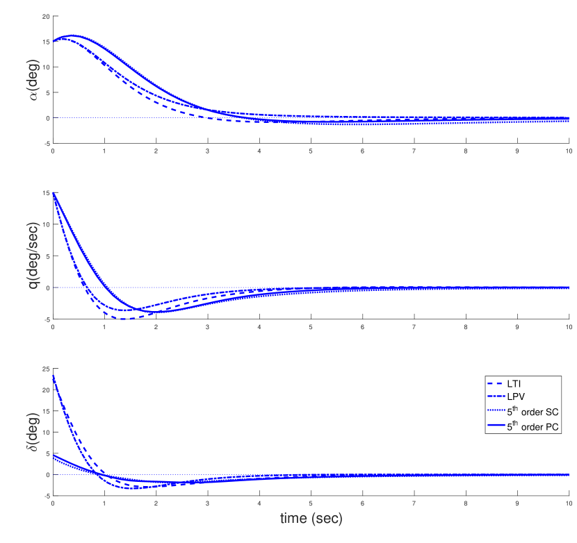
Figure 1: State and control trajectories for the missile autopilot by applying different controllers.

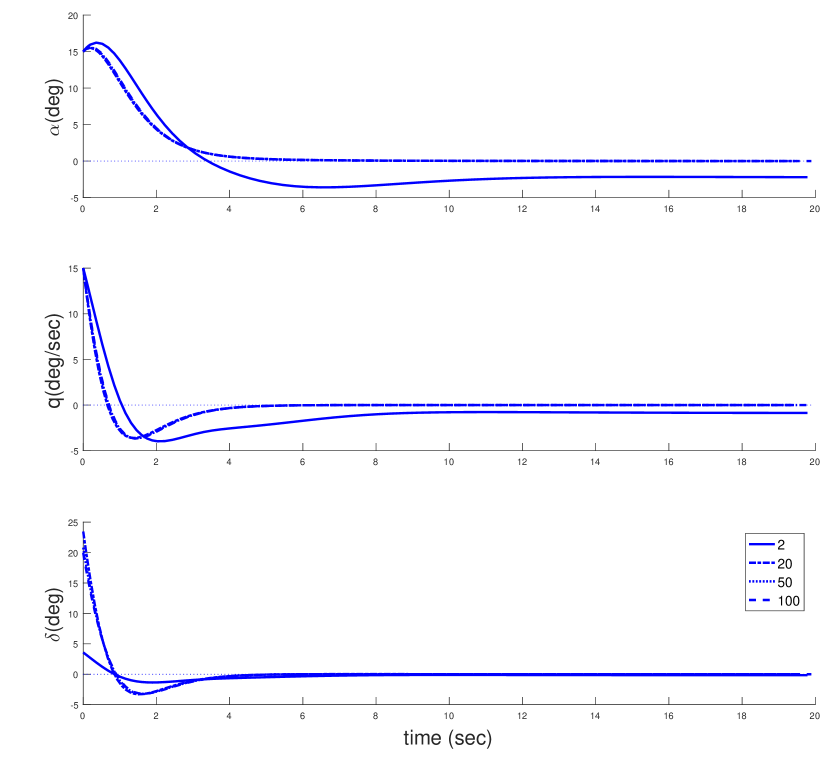
Figure 2: State and control trajectories for the missile autopilot by applying LPV control with different sample points.

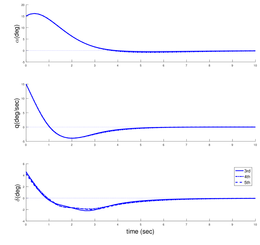
Figure 3: State and control trajectories for the missile autopilot by applying pcLPV control with different order polynomial chaos expansion.

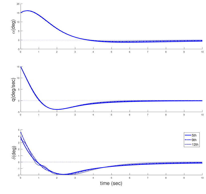
Figure 4: State and control trajectories for the missile autopilot by applying scLPV control with different sample points.

References

[1]
Jeff S Shamma.
An overview of lpv systems.
In Control of Linear Parameter Varying Systems with
Applications, pages 3–26. Springer, 2012.
[2]
Douglas J Leith and William E Leithead.
Survey of gain-scheduling analysis and design.
International journal of control, 73(11):1001–1025, 2000.
[3]
Onur Toker.
On the complexity of the robust stability problem for linear
parameter varying systems.
Automatica, 33(11):2015–2017, 1997.
[4]
Yasumasa Fujisaki, Fabrizio Dabbene, and Roberto Tempo.
Probabilistic design of lpv control systems.
Automatica, 39(8):1323–1337, 2003.
[5]
N. Wiener.
The homogeneous chaos.
American Journal of Mathematics, 60(4):897–936, October 1938.
[6]
V. Volterra.
Lecons sur les Equations Integrales et Integrodifferentielles.
Paris: Gauthier Villars, 1913.
[7]
Roger G. Ghanem and Pol D. Spanos.
Stochastic Finite Elements: A Spectral Approach.
Springer-Verlag New York, Inc., New York, NY, USA, 1991.
[8]
R. H. Cameron and W. T. Martin.
The Orthogonal Development of Non-Linear Functionals in Series of
Fourier-Hermite Functionals.
The Annals of Mathematics, 48(2):385–392, 1947.
[9]
Dongbin Xiu and George Karniadakis.
The Wiener–askey polynomial chaos for stochastic differential
equations.
SIAM Journal on Scientific Computing, 24(2):619–644, 2002.
[10]
R. Askey and J. Wilson.
Some Basic Hypergeometric Polynomials that Generalize Jacobi
Polynomials.
Memoirs Amer. Math. Soc., 319, 1985.
[11]
Thomas Y. Hou, Wuan Luo, Boris Rozovskii, and Hao-Min Zhou.
Wiener Chaos Expansions and Numerical Solutions of Randomly Forced
Equations of Fluid Mechanics.
J. Comput. Phys., 216(2):687–706, 2006.
[12]
Dongbin Xiu and George Em Karniadakis.
Modeling Uncertainty in Flow Simulations via Generalized Polynomial
Chaos.
J. Comput. Phys., 187(1):137–167, 2003.
[13]
Xiaoliang Wan, Dongbin Xiu, and George Em Karniadakis.
Stochastic solutions for the two-dimensional advection-diffusion
equation.
SIAM J. Sci. Comput., 26(2):578–590, 2005.
[14]
Roger Ghanem and John Red-Horse.
Propagation of Probabilistic Uncertainty in Complex Physical Systems
Using a Stochastic Finite Element Approach.
Phys. D, 133(1-4):137–144, 1999.
[15]
R.G. Ghanem.
Ingredients for a General Purpose Stochastic Finite Elements
Implementation.
Comput. Methods Appl. Mech. Eng., 168(1-4):19–34, 1999.
[16]
Franz S Hover and Michael S Triantafyllou.
Application of polynomial chaos in stability and control.
Automatica, 42(5):789–795, 2006.
[17]
K.K Kim and R. D Braatz.
Generalized polynomial chaos expansion approaches to approximate
stochastic receding horizon control with applications to probabilistic
collision checking and avoidance.
In Control Applications (CCA), 2012 IEEE International
Conference on, pages 350–355. IEEE, 2012.
[18]
James Fisher and Raktim Bhattacharya.
Linear quadratic regulation of systems with stochastic parameter
uncertainties.
Automatica, 45(12):2831–2841, 2009.
[19]
R. Bhattacharya and J. Fisher.
Linear receding horizon control with probabilistic system parameters.
In Robust Control Design, volume 7, pages 627–632, 2012.
[20]
Parikshit Dutta and Raktim Bhattacharya.
Nonlinear Estimation with Polynomial Chaos and Higher Order Moment
Updates.
In 2010 American Control Conference, Marriott Waterfront, pages
3142–3147, Baltimore, MD, USA, 2010.
[21]
Olivier P Le Maître and Omar M Knio.
Spectral methods for uncertainty quantification: with
applications to computational fluid dynamics.
Springer, 2010.
[22]
MS Eldred and John Burkardt.
Comparison of non-intrusive polynomial chaos and stochastic
collocation methods for uncertainty quantification.
AIAA paper, 976(2009):1–20, 2009.
[23]
R. A. Horn and C. R. Johnson.
Topics in Matrix Analysis.
Cambridge university press, 2012.
[24]
Carsten W Scherer and Camile WJ Hol.
Matrix sum-of-squares relaxations for robust semi-definite programs.
Mathematical programming, 107(1-2):189–211, 2006.
[25]
Fen Wu, Andy Packard, and Gary Balas.
Lpv control design for pitch-axis missile autopilots.
In Decision and Control, 1995., Proceedings of the 34th IEEE
Conference on, volume 1, pages 188–193. IEEE, 1995.
[26]
The Math Works.
MATLAB: High Performance Numeric Computation and
Visualization Software, 1992.
[27]
Michael Grant, Stephen Boyd, and Yinyu Ye.
Cvx: Matlab software for disciplined convex programming, 2008.