SHOPPER: A Probabilistic Model of Consumer Choice with Substitutes and Complements

Francisco J. R. Ruizlabel=e1]f.ruiz@columbia.edu [ Susan Atheylabel=e2]athey@susanathey.com [ David M. Bleilabel=e3]david.blei@columbia.edu [ University of Cambridge,\thanksmarkm1 Columbia University,\thanksmarkm2 and Stanford University\thanksmarkm3

We develop shopper, a sequential probabilistic model of shopping data. shopper uses interpretable components to model the forces that drive how a customer chooses products; in particular, we designed shopper to capture how items interact with other items. We develop an efficient posterior inference algorithm to estimate these forces from large-scale data, and we analyze a large dataset from a major chain grocery store. We are interested in answering counterfactual queries about changes in prices. We found that shopper provides accurate predictions even under price interventions, and that it helps identify complementary and substitutable pairs of products.

\startlocaldefs\endlocaldefs

, and

1 Introduction

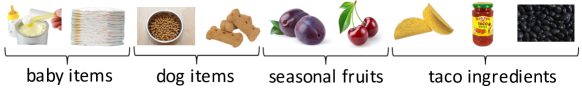
Large-scale shopping cart data provides unprecedented opportunities for researchers to understand consumer behavior and to predict how it responds to interventions such as promotions and price changes. Consider the shopping cart in Figure 1. This customer has purchased items for their baby (diapers, formula), their dog (dog food, dog biscuits), some seasonal fruit (cherries, plums), and the ingredients for tacos (taco shells, salsa, and beans). Shopping cart datasets may contain thousands or millions of customers like this one, each engaging in dozens or hundreds of shopping trips.

In principle, shopping cart datasets could help reveal important economic quantities about the marketplace. They could help evaluate counterfactual policies, such as how changing a price of a product will affect the demand for it and for other related products; and they could help characterize consumer heterogeneity, which would allow firms to consider different interventions for different segments of their customers. However, large-scale shopping cart datasets are too complex and heterogenous for classical methods of analysis, which necessarily prune the data to a handful of categories and a small set of customers. In this paper, our goal is to develop a method that can usefully analyze large collections of complete shopping baskets.

Shopping baskets are complex because, as the example shopper in Figure 1 demonstrates, many interrelated forces are at play when determining what a customer decides to buy. For example, the customer might consider how well the items go together, their own personal preferences and needs (and whims), the purpose of the shopping trip, the season of the year, and, of course, the prices and the customer’s personal sensitivity to them. Moreover, these driving forces of consumer behavior are unobserved elements of the market. Our goal is to extract them from observed datasets of customers’ final purchases.

To this end we develop shopper, a sequential probabilistic model of market baskets. shopper uses interpretable components to model the forces that drive customer choice, and we designed shopper to capture properties of interest regarding how items interact with other items; in particular, we are interested in answering counterfactual queries with respect to item prices. We also develop an efficient posterior inference algorithm to estimate these forces from large-scale data. We demonstrate shopper by analyzing data from a major chain grocery store (Che, Chen and Chen, 2012). We found that shopper provides accurate predictions even under price interventions, and that it also helps identifying complementary and substitutable pairs of items.

Refer to caption — Figure 1: An example of a shopping cart, generated under several underlying interrelated forces (customer needs, availability of seasonal fruits, complementary sets of items).

1.1 Main idea

shopper is a hierarchical latent variable model of market baskets for which the generative process comes from an assumed model of consumer behavior. In the language of social science, shopper is a structural model of consumer behavior, where the elements of the model include the specification of consumer preferences, information, and behavior (i.e., utility maximization). In the language of probabilistic models, it can equivalently be defined by a generative model.

shopper posits that a customer walks into the store and chooses items sequentially. Further, the customer might decide to stop shopping and pay for the items; this is the “checkout” item. At each step, the customer chooses among the previously unselected items, while conditioning on the items already in the basket. The customer’s choices also depend on various other aspects: the prices of the items and the customer’s sensitivities to them, the season of the year, and the customer’s general shopping preferences (which are specific for each customer).

One key feature of shopper is that each possible item is associated with latent attributes $\alpha_{c}$ , vector representations that are learned from the data. This is similar in spirit to methods from machine learning that estimate semantic attributes of vocabulary words by analyzing the words close to them in sentences (Bengio et al., 2003). In shopper “words” are items and “sentences” are baskets of purchased items.

shopper uses the latent attributes in two ways. First, they help represent the existing basket when considering which item to select next. Specifically, each possible item is also associated with a vector of interaction coefficients $\rho_{c}$ , parameters that represent which kinds of basket-level attributes it tends to appear with. For example, the interaction coefficients and attributes can capture that when taco shells are in the basket, the customer has a high probability of choosing taco seasoning. Second, they are used as the basis for representing customer preferences. Each customer in the population also has a vector of interaction coefficients $\theta_{u}$ , which we call “preferences,” that represent the types of items that they tend to purchase. For example, the customer preferences and attributes can capture that some customers tend to purchase baby items or dog food.

Mathematically, at the $i$ th step of the sequential process, the customer chooses item $c$ with probability that depends on the latent features of item $c$ , on her preferences $\theta_{u}$ , and on the representation of the items that are already in the basket, $\sum_{j=1}^{i-1}\alpha_{y_{j}}$ (where $y_{j}$ indicates the item purchased at step $j$ ). In its vanilla form, shopper posits that this probability takes a log-bilinear form,

\displaystyle\textrm{Prob}(\textrm{item }c\,|\,\textrm{items in basket})\propto\exp\left\{\theta_{u}^{\top}\alpha_{c}+\rho_{c}^{\top}\left(\frac{1}{i-1}\sum_{j=1}^{i-1}\alpha_{y_{j}}\right)\right\}.

(1)

Section 2 provides more details about the model and also describes how to incorporate price and seasonal effects.

When learned from data, the latent attributes $\alpha_{c}$ capture meaningful dimensions of the data. For example, Figure 2 illustrates a two-dimensional projection of learned latent item attributes. Similar items are close together in the attribute space, even though explicit attributes (such as category or purpose) are not provided to the algorithm.

In the simplest shopper model, the customer is myopic: at each stage they do not consider that they may later add additional items into the basket. This assumption is problematic when items have strong interaction effects, since it is likely that a customer will consider other items that complement the currently chosen item. For example, if a customer considers purchasing taco seasoning, they should also consider that they will later want to purchase taco shells.

To relax this assumption, we include a second key feature of shopper, called “thinking ahead,” where the customer considers the next choice in making the current choice. For example, consider a scenario where taco shells have an unusually high price and where the customer is currently contemplating putting taco seasoning in the basket. As a consequence of thinking ahead, the model dampens the probability of choosing seasoning because of the high price of its likely complement, taco shells. shopper models one step of thinking ahead. (It may be plausible in some settings that customers think further ahead when shopping; we leave this extension for future work.)

1.2 Main results

We fit shopper to a large data set of market baskets, estimating the latent features of the items, seasonal effects, preferences of the customers, and price sensitivities. We evaluate the approach with held-out data, used in two ways. First, we hold out items from the data at random and assess their probability with the posterior predictive distribution. This checks how well shopper (and our corresponding inference algorithm) captures the distribution of the data. Second, we evaluate on held-out baskets in which items have larger price variation compared to their average values. This evaluation assesses how well shopper can evaluate counterfactual price changes. With both modes of evaluation, we found shopper gave better predictions than state-of-the-art econometric choice models and machine learning models for item consumption, which are based on either user/item factorization, such as factor analysis or Poisson factorization (Gopalan, Hofman and Blei, 2015), or on item/item factorization, such as exponential family embeddings (Rudolph et al., 2016).

Further, shopper can help identify pairs of items that are substitutes and complements—where purchasing one item makes the second item less or more attractive, respectively. This is one of the fundamental challenges of analyzing consumer behavior data. Formally, two items are complements if the demand of one is increased when the price of the other decreases; they are substitutes if the demand for one rises when the price of the other item increases. Studying complementary and substitutable items is key to make predictions about the (joint) demand.

Notice that being complements is more than the propensity for two items to be co-purchased; items may be purchased together for many reasons. As one reason, two items may be co-purchased because people who like one item tend to also like the other item. For example, baby formula and diapers are often co-purchased but they are not complements—when baby formula is unavailable at the store, it does not affect the customer’s preference for diapers.

shopper can disentangle complementarity from other sources of co-purchase because prices change frequently in the dataset. If two items are co-purchased but not complements, increasing the price of one does not decrease the purchase rate of the other. Using the item-to-item interaction term in shopper, we develop a measure to quantify how complementary two items are. (In this sense, shopper corroborates the theory of Athey and Stern (1998) among others, who show that if there is sufficient variation in the price of each item then it is theoretically possible to separate correlated preferences from complementarity.)

Now we turn to substitutes, where purchasing one item decreases the utility of another, e.g., two brands of (otherwise similar) taco shells. Although in principle substitutes can be treated symmetrically to complements (increasing the price of one brand of taco shells increases the probability that the other is purchased if they are substitutes), in practice the two concepts are not equally easy to discover in the data. The difference is that in most shopping data, purchase probabilities are very low for all items, and so most pairs of items are rarely purchased together. In this paper, we introduce an alternative way to find relationships among products, “exchangability.” Two products are exchangeable if they tend to have similar pairwise interactions with other products; for example, two brands of taco shells would have similar interactions with products such as tomatoes and beans. Of course, products that are usually purchased together, like hot dogs and buns, will also have similar pairwise interactions with other products (such as ketchup). Our results suggest that items that are exchangeable and not complementary tend to be substitutes (in the sense of being in the same general product category in the grocery store hierarchy).

2 A Bayesian model of sequential discrete choice

We develop shopper, a sequential probabilistic model of market baskets. shopper treats each choice as one over the set of available items, where the attributes of each item are latent variables.

We describe shopper in three stages. Section 2.1 describes a basic model of sequential choice with latent item attributes; Section 2.2 extends the model to capture user heterogeneity, seasonal effects, and price; Section 2.3 develops “thinking ahead,” where we model each choice in a way that considers the next choice as well.

shopper comes with significant computational challenges, both because of its complex functional form and the size of the data that we would like to analyze. We defer these challenges to Section 5, where we develop an efficient variational algorithm for approximate posterior inference.

2.1 Sequential choice with latent item attributes

We describe the basic model in terms of its generative process or, in the language of economics and marketing, in terms of its structural model of consumer behavior. Each customer walks into the store and picks up a basket. She chooses items to put in the basket, one by one, each one conditional on the previous items in the basket. The process stops when she purchases the “checkout” item, which we treat as a special item that ends the trip.

From the utility-maximizing perspective, shopper works as follows. First, the customer walks into the store and obtains utilities for each item. She considers all of the items in the store and places the highest-utility item in her basket. In the second step, once the first item is in the basket, the customer again considers all remaining items in the store and selects the highest-utility choice. However, relative to the first decision, the utilities of the products change. First, the specification of the utility allows for interaction effects—items may be substitutes (e.g., two brands of taco seasoning) or complements (e.g., taco shells and taco seasoning), in the sense that the utility of an item may be higher or lower as a result of having the first item in the basket. Second, the customer’s utilities have a random component that changes as she shops. This represents, for example, changing ideas about what is needed, or different impressions of products when reconsidering them. (Another extension of the model would be to allow for correlation of the random component over choice events within a shopping trip; we leave this for future work.) The customer repeats this process—adjusting utilities and choosing the highest-utility item among what is left in the store—until the checkout item is the highest-utility item.

In some applications, it may not be reasonable to model the consumer as considering all items. In a supermarket, a customer might consider one part of the store at the time; in an online store, a customer may only consider the products that appear in a search results page. Corresponding extensions to shopper are straightforward but, for simplicity, we do not include them here. Modeling customers as choosing the most desirable items in the store first ensures that, among goods that are close substitutes, they select the most desirable one.

We describe the sequential choice model more formally. Consider the $t$ th trip and let $n_{t}$ be the number of choices, i.e., the number of purchased items. Denote the (ordered) basket $\mathbf{y}_{t}=(y_{t1},\ldots,y_{tn_{t}})$ , where each $y_{ti}$ is one of $C$ items and choice $y_{tn_{t}}$ is always the checkout item. Let $\mathbf{y}_{t,i-1}$ denote the items that are in the basket up to position $i$ , $\mathbf{y}_{t,i-1}=(y_{t1},\ldots,y_{t,i-1})$ .

Consider the choice of the $i$ th item. The customer makes this choice by selecting the item $c$ that has maximal utility $U_{t,c}(\mathbf{y}_{t,i-1})$ , which is a function of the items in the basket thus far. The utility of item $c$ is

\displaystyle U_{t,c}(\mathbf{y}_{t,i-1})=\Psi(c,\mathbf{y}_{t,i-1})+\epsilon_{t,c}.

(2)

Here $\Psi(c,\mathbf{y}_{t,i-1})$ is the deterministic part of the utility, a function of the other items in the basket. We define $\Psi(c,\mathbf{y}_{t,i-1})\equiv-\infty$ for $c\in\mathbf{y}_{t,i-1}$ , so that the choice is effectively over the set of non-purchased items. The random variable $\epsilon_{t,c}$ is assumed to follow a zero-mean Gumbel distribution (generalized extreme value type-I), which is independent across items.

This behavioral rule—and particularly the choice of Gumbel error terms—implies that the conditional choice probability of an item $c$ that is not yet in the basket is a softmax,

\displaystyle p(y_{ti}=c\,|\,\mathbf{y}_{t,i-1})=\frac{\exp\{\Psi(c,\mathbf{y}_{t,i-1})\}}{\sum_{c^{\prime}\not\in\mathbf{y}_{t,i-1}}\exp\{\Psi(c^{\prime},\mathbf{y}_{t,i-1})}.

(3)

Notice the denominator is a sum over a potentially large number of items. For example, Section 6 analyzes data with nearly six thousand items. Section 5 describes fast methods for handling this computational bottleneck.

Eq. 3 gives a model of observed shopping trips, from which we can infer the utility function. The core of shopper is in the unnormalized log probabilities $\Psi(c,\mathbf{y}_{t,i-1})$ , which correspond to the mean utilities of the items. We assume that they have a log-linear form,

\displaystyle\Psi(c,\mathbf{y}_{t,i-1})=\psi_{tc}+\rho_{c}^{\top}\left(\frac{1}{i-1}\sum_{j=1}^{i-1}\alpha_{y_{tj}}\right).

(4)

There are two terms. The first term $\psi_{tc}$ is a latent variable that varies by item and by trip; below we use this term to capture properties such as user heterogeneity, seasonality, and price. We focus now on the second term, which introduces two important latent variables: the per-item interaction coefficients $\rho_{c}$ and the item attributes $\alpha_{c}$ , both real-valued $K$ -vectors. When $\rho_{c}^{\top}\alpha_{c^{\prime}}$ is large, then having $c^{\prime}$ in the basket increases the benefit to the customer of placing $c$ in the basket (the items are complements in the customer’s utility); conversely, when the expression is negative, the items are substitutes.

Unlike traditional factorization methods, the factorization is asymmetric. We interpret $\alpha_{c}$ as latent item characteristics or attributes; we interpret $\rho_{c}$ as the interaction of item $c$ with other items in the basket, as described by their attributes (i.e., their $\alpha$ ’s). These interactions allow that even though two items might be different in their latent attributes (e.g., taco shells and beans), they still may be co-purchased because they are complements to the consumer. It can also capture that similar items (e.g., two different brands of the same type of taco seasoning) may explicitly not be purchased together—these are substitutable items. Below we also allow that the latent attributes $\alpha_{c}$ further affect the item’s latent mean utility on the trip $\psi_{tc}$ .

We also note that the second term has a scaling factor, $1/(i-1)$ . This scaling factor captures the idea that in a large basket, each individual item has a proportionally smaller interaction with new purchases. This may be a more reasonable assumption in some scenarios than others, exploring alternative ways to account for basket size is a direction for future work.

Finally, note we assumed that $\Psi(\cdot)$ is additive in the other items in the basket. With an additive model, the interaction term $\rho_{c}^{\top}\alpha_{c^{\prime}}$ affects the probability of item $c$ in the same way for each item $c^{\prime}$ in the basket. In addition, this choice rules out non-linear interactions with other items. Again, this restriction may be more realistic in some applications than in others, but it is possible to extend the model to consider more complex interaction patterns if necessary. In this paper, we only consider linear interaction effects.

2.1.1 Baskets as unordered set of items

Given Eq. 3, the probability of an ordered basket is the product of the individual choice probabilities. Assuming that $y_{tn_{t}}$ is the checkout item, it is

\displaystyle p(\mathbf{y}_{t}\,|\,\rho,\alpha)=\prod_{i=1}^{n_{t}}p(y_{ti}\,|\,\mathbf{y}_{t,i-1},\rho,\alpha).

(5)

The probabilities come from Eq. 3 and Eq. 4, and we have made explicit the dependence on the interaction coefficients and item attributes. The parameters of this softmax are determined by the interaction vectors $\rho_{c}$ and the attributes $\alpha_{c}$ of the items that have already been purchased. Given a dataset of (ordered) market baskets, we can use this likelihood to fit each item’s latent attributes and interaction.

In many datasets, however, the order in which the items are added to the basket is not observed. shopper implies the likelihood of an unordered set $\mathpzc{y}_{t}$ by summing over all possible orderings,

\displaystyle p(\mathpzc{y}_{t}\,|\,\rho,\alpha)=\sum_{\pi}p(\mathbf{y}_{t,\pi}\,|\,\rho,\alpha).

(6)

Here $\pi$ is a permutation (with the checkout item fixed to the last position) and $\mathbf{y}_{t,\pi}$ is the permuted basket $(y_{t,\pi_{1}},\ldots,y_{t,\pi_{n_{t}}})$ . Its probability is in Eq. 5. In Section 6, we study a large dataset of unordered baskets; this is the likelihood that we use when fitting shopper.

2.1.2 Utility maximization of baskets

Here we describe how the sequential model behind shopper relates to a utility maximization model over unordered sets of items, in which the customer has a specific utility for each basket (i.e., with $2^{C}$ choices, where $C$ is the number of items).

Let $\mathpzc{y}_{t}$ be the (unordered) set of items purchased in trip $t$ . Define a consumer’s utility over unordered baskets as follows:

\displaystyle\widetilde{U}_{t}(\mathpzc{y}_{t})=\sum_{c\in\mathpzc{y}_{t}}{\psi_{tc}}+\frac{1}{|\mathpzc{y}_{t}|-1}\sum_{(c,c^{\prime})\in\mathpzc{y}_{t}\times\mathpzc{y}_{t}:c^{\prime}\neq c}{\nu_{c,c^{\prime}}},

(7)

where $\nu_{c,c^{\prime}}$ is a term that describes the interaction between $c$ and $c^{\prime}$ . Now consider the following model of utility maximization. At each stage where a consumer must select an item, the consumer has an extreme form of myopia, whereby she assumes that she will immediately check out after selecting this item, and she does not consider the possibility that she could put any items in her basket back on the shelf. Other than this myopia, she behaves rationally, maximizing her utility over unordered items as given by Eq. 7.

The behavioral model of sequential shopping is consistent with the myopic model of utility maximization if (and only if) $\nu_{c,c^{\prime}}=\rho_{c}^{\top}\alpha_{c^{\prime}}=\rho_{c^{\prime}}^{\top}\alpha_{c}$ ; this says that the impact of product $c$ on the purchase of product $c^{\prime}$ is symmetric to the impact of $c$ on product $c^{\prime}$ , holding fixed the rest of the basket. (We do not impose such a symmetry constraint in our model because of the reasons outlined in Eq. 4.) Thus, we can think of utility maximization by this type of myopic consumer as imposing an additional constraint on the probabilistic model. This follows the common practice in economic modeling to estimate the richer models motivated by theory, but without imposing all the restrictions on the parameters implied by that theory; this approach often simplifies computation. Browning and Meghir (1991) also estimate an econometric model without imposing symmetry restrictions implied by utility maximization, and then impose the restrictions in a second step using a minimum-distance approach.

Finally, we note that a fully rational consumer with full information of the price of all products could in principle consider all of the possible bundles in the store simultaneously and maximize over them. However, given that the number of bundles is $2^{C}$ , we argue that considering such a large number of bundles simultaneously is probably not a good approximation to human behavior. Even if consumers are not as myopic as we assume, it is more realistic to assume that they follow some simple heuristics.

2.2 Preferences, seasons, popularity, and price

The basic shopper model of the previous section captures a customer’s sequential choices as a function of latent attributes and interaction coefficients. shopper is flexible, however, in that we can include other forces in the model of customer choice; specifically, they can be incorporated into the (unobserved) mean utility of each item $c$ , $\psi_{tc}$ , which varies with trip and customer. Here we describe extensions to capture item popularity, customer preferences, price sensitivity, and seasonal purchasing habits (e.g., for holidays and growing seasons). All these factors are important when modeling real-world consumer demand.

2.2.1 Item popularity

We capture overall (time-invariant) item popularity with a latent intercept term $\lambda_{c}$ for each item. When inferred from data, popular items will have a high value of $\lambda_{c}$ , which will generally increase their choice probabilities.

2.2.2 Customer preferences

In our data, each trip $t$ is associated with a particular customer $u_{t}$ , and that customer’s preferences affect her choices. We model preference with a per-customer latent vector $\theta_{u}$ . For each choice, we add the inner product $\theta_{u}^{\top}\alpha_{c}$ to the unnormalized log probability of each item. This term increases the probability of types of items that the customer tends to purchase. Recall that $\theta_{u}$ is a per-customer variable that appears in every shopping trip $t$ involving customer $u$ . Note that shopper shares the attributes $\alpha_{c}$ with the part of the model that characterizes interaction effects. The inference algorithm finds latent attributes $\alpha_{c}$ that interact with both customer preferences and also with other items in the basket.

2.2.3 Price sensitivity

We next include per-customer price sensitivity. Let $r_{tc}$ denote the price of item $c$ at trip $t$ . We consider each customer has an individualized price sensitivity to each item, denoted $\tau_{uc}$ , and we add the term $-\tau_{uc}\log r_{tc}$ to the unnormalized log probabilities in Eq. 4. We place a minus sign in the price term to make the choice less likely as the price $r_{tc}$ increases. Further, we constrain $\tau_{uc}$ to be positive; this constraint ensures that the resulting price elasticities are negative. (The price elasticity of demand $\varepsilon$ is a measure used in economics to show the responsiveness of the quantity demanded of a good $y$ to a change in its price $r$ ; it is defined as $\varepsilon=\partial\log y/\partial\log r$ .)

Including $\tau_{uc}$ posits a large number of latent variables (for many customers and items) and, moreover, it is reasonable to assume the sensitivities will be correlated, e.g., a customer’s sensitivity to peanut butter and almond butter might be similar. Thus we use a matrix factorization to model the price sensitivities. Specifically, we decompose the user/item price sensitivity matrix into per-user latent vectors $\gamma_{u}$ and per-item latent vectors $\beta_{c}$ , where $\tau_{uc}=\gamma_{u}^{\top}\beta_{c}$ . This factorization models the complete matrix of price sensitivities with fewer latent variables.

Finally, instead of the raw price $r_{tc}$ , we use the normalized price, i.e., the price for this trip divided by the per-item mean price. Normalized prices have two attractive properties. First, they allow $\beta_{c}$ to be on a comparable scale, avoiding potential issues that arise when different items have prices that vary by orders of magnitude. Second, they ensure that the other parameters in Eq. 4 capture the average outcome distribution: the price term vanishes when the price takes its average value because the log of the normalized price is zero.

2.2.4 Seasonal effects

We complete the model with seasonal effects. shopper is designed to estimate the effect of counterfactual changes in policy, such as prices. So, it is important that the parameters of the model associated with price represent the true causal effect of price on customer choices. Seasonal effects are a potential confounder—the season simultaneously affects the price and the demand of an item—and so neglecting to control for seasonality can lead to estimates of the latent variables that cannot isolate the effects of changing prices. For example, the demand for candy goes up around Halloween and the supermarket may decide to put candy on sale during that period. The demand increases partly because of the price, but also because of the time of year. Controlling for seasonal effects isolates the causal effect of price.

We assume that seasonal effects are constant for each calendar week and, as for the price effect, we factorize the week-by-item seasonal effects matrix. (This is motivated by Donnelly et al. (2019), who conduct a series of empirical studies that support the idea that controlling for week effects is sufficient to identify the causal effect of price.) Denote the week of trip $t$ as $w_{t}\in\{1,\ldots,52\}$ . We posit per-week latent vectors $\delta_{w}$ and per-item latent vectors $\mu_{c}$ , and we include a term in Eq. 4 that models the effect of week $w$ on item $c$ ’s probability, $\delta_{w}^{\top}\mu_{c}$ . Note this allows correlated seasonal effects across items; items with similar $\mu_{c}$ vectors will have similar seasonal effects. So Halloween candy and pumpkin cookies might share similar $\mu_{c}$ vectors.

2.2.5 Putting it together

We described popularity, preferences, price, and season. We combine these effects in the per-item per-trip latent variable $\psi_{tc}$ ,

\displaystyle\psi_{tc}=\underbrace{\lambda_{c}}_{\textrm{item popularity}}+\underbrace{\theta_{u_{t}}^{\top}\alpha_{c}}_{\textrm{customer preferences}}-\underbrace{\gamma_{u_{t}}^{\top}\beta_{c}\log r_{tc}}_{\textrm{price effects}}+\underbrace{\delta_{w_{t}}^{\top}\mu_{c},}_{\textrm{seasonal effects}}

(8)

where the subscripts $u_{t}$ and $w_{t}$ indicate, respectively, the customer and week corresponding to shopping trip $t$ . The mean utility $\psi_{tc}$ is used in the probabilities for all $n_{t}$ choices of trip $t$ . With these extensions we have introduced several new latent variables to infer from data: item popularities $\lambda_{c}$ , customer preferences $\theta_{u}$ , price sensitivity factorizations $\gamma_{u}$ and $\beta_{c}$ , and seasonal factorizations $\delta_{w}$ and $\mu_{c}$ .

2.3 Thinking ahead

As a final extension, we develop a model of customers that “think ahead.” Consider a pair of items $c$ and $c^{\prime}$ , where both $\rho_{c}^{\top}\alpha_{c^{\prime}}$ and $\rho_{c^{\prime}}^{\top}\alpha_{c}$ are high, so that the value of $c$ increases when $c^{\prime}$ is in the basket and vice versa. In this case, we say that the goods are complements to the consumer. Accurately accounting for complementarity is particularly important when estimating counterfactuals based on different prices; theoretically increasing the price of one item should lower the probability of the other.

In this scenario, our baseline model specifies that the consumer will consider the goods one at a time. The effect of a high price for item $c^{\prime}$ is that it reduces the probability the item is chosen (and if chosen, it is less likely to be chosen early in the ordering). Not having item $c^{\prime}$ in the basket at each new consideration event reduces the attractiveness of item $c$ . However, a more realistic model has the consumer anticipate when she considers item $c$ that she might also consider item $c^{\prime}$ . When the consumer considers the pair, the high price of one item deters the purchase of both.

We address this issue by introducing thinking ahead. When considering the item at step $i$ , the consumer looks ahead at the $i+1$ th step the customer may purchase. We emphasize that the model does not, at this point, assume that the consumer actually purchases the next item according to that rule. When the consumer comes to consider what to choose for step $i+1$ , she follows the same think-ahead-one-step rule just described.

Thinking ahead adjusts the unnormalized log probabilities of the current item in Eq. 4. Specifically, it adds a term to the log linear model that is the utility of the optimal next item. (Note this could be the checkout item.) The unnormalized log probability is

\displaystyle\begin{aligned} \Psi(c,\mathbf{y}_{t,i-1})=&\psi_{tc}+\rho_{c}^{\top}\left(\frac{1}{i-1}\sum_{j=1}^{i-1}\alpha_{y_{tj}}\right)\\ &\qquad+\max_{c^{\prime}\not\in[\mathbf{y}_{t,i-1},c]}\left\{\psi_{tc^{\prime}}+\rho_{c^{\prime}}^{\top}\left(\frac{1}{i}\left(\alpha_{c}+\sum_{j=1}^{i-1}\alpha_{y_{tj}}\right)\right)\right\},\end{aligned}

(9)

where $[\mathbf{y}_{t,i-1},c]$ is a hypothetical basket that contains the first $i-1$ purchased items and item $c$ . Since the customer has in mind a tentative next item when deciding about the current item, we call this “thinking one step ahead.”

Note that thinking ahead assumes that the item $c^{\prime}$ will itself be selected without looking further ahead, that is, it is chosen purely based on its own utility without accounting for the interaction effects of $c^{\prime}$ with future purchases. The thinking-ahead idea can be extended to two or more steps ahead, but at the expense of a higher computational complexity. See Section 3 for an illustrative example that clarifies how the thinking-ahead procedure works.

The thinking-ahead mechanism is an example of inferring agent’s preferences from their behavior in a dynamic model, a type of exercise with a long history in applied econometrics (e.g. Wolpin (1984); Hotz and Miller (1993)). From the machine learning perspective, it closely resembles the motivation behind inverse reinforcement learning (Russell, 1998; Ng and Russell, 2000). Inverse reinforcement learning analyzes an agent’s behavior in a variety of circumstances and aims to learn its reward function. (This is in contrast to reinforcement learning, where the reward function is given.) To see the connection, consider the unnormalized log probability of Eq. 9 as the reward for choosing $c$ and then acting optimally one step (i.e., choosing the best next item). With this perspective, fitting shopper to observed data is akin to learning the reward function.

Finally, note the thinking-ahead model also connects to utility maximization over unordered baskets, with the utility function given in Eq. 7. Now the model is consistent with a consumer who maximizes her utility over unordered items at each step, but where at each step she is myopic in two ways. First, as before, she does not consider that she can remove items from her cart. Second, she assumes that she will buy exactly one more item in the store and then check out, and the next item will be the one that maximizes her utilty over unordered baskets (taking as given her cart at that point, including the latest item added, as well as the belief that she will then check out). Again, our probabilistic model is consistent with this interpretation if and only if $\rho_{c^{\prime}}^{\top}\alpha_{c}=\rho_{c}^{\top}\alpha_{c^{\prime}}$ for all $(c,c^{\prime})$ (a constraint that we do not enforce).

2.4 Full model specification

We specified shopper, a sequential model of shopping trips. Each trip is a tuple $(\mathbf{y}_{t},u_{t},w_{t},r_{t})$ containing a collection of purchased items ( $\mathbf{y}_{t}$ ), the customer who purchased them ( $u_{t}$ ), the week that the shopping trip took place ( $w_{t}$ ), and the prices of all items ( $r_{t}$ ). The likelihood of each shopping trip captures the sequential process of the customer choosing items (Eq. 3), where each choice is a log linear model (Eq. 4). shopper includes terms for item popularity, customer preferences, price sensitivity, and seasonal effects (Eq. 8). We further described a variant that models the customer thinking ahead and acting optimally (Eq. 9). Though this is a model of ordered baskets, we can use it to evaluate the probability of an unordered basket of items (Eq. 6).

shopper is based on log linear terms that involve several types of latent parameters: per-item interaction coefficients $\rho_{c}$ , per-item attributes $\alpha_{c}$ , per-item popularities $\lambda_{c}$ , per-user preferences $\theta_{u}$ , per-user per-item price sensitivities $(\gamma_{u},\beta_{c})$ , and per-week per-item seasonal effects $(\delta_{w},\mu_{c})$ . Our goal is to estimate these parameters given a large data set of $T$ trips $\{(\mathbf{y}_{t},u_{t},w_{t},r_{t})\}_{t=1}^{T}$ .

We take a Bayesian approach. We place priors on the parameters to form a Bayesian model of shopping trips, and then we form estimates of the latent parameters by approximating the posterior. We use independent Gaussian priors for the real-valued parameters, $\rho_{c}$ , $\alpha_{c}$ , $\theta_{u}$ , $\lambda_{c}$ , $\delta_{w}$ , and $\mu_{c}$ . We use gamma priors for the positive-valued parameters associated with price sensitivity, $\gamma_{u}$ and $\beta_{c}$ . With the approximate posterior, we can use the resulting estimates to identify various types of purchasing patterns and to make predictions about the distribution of market baskets; in particular predictions under price changes.

Finally, note that shopper uses matrix factorization approaches for customer preferences ( $\theta_{u}^{\top}\alpha_{c}$ ), price effects ( $\gamma_{u}^{\top}\beta_{c}$ ), and seasonal effects ( $\delta_{w}^{\top}\mu_{c}$ ). Matrix factorization has two sources of invariance (label switching and rescaling). This implies that we cannot uniquely identify individual variables such as $\theta_{u}$ or $\gamma_{u}$ from the data. Fortunately, this is not an issue for (counterfactual) predictions, because they only depend on the inner products and not on the individual coefficients.

3 Illustrative simulation

We now describe a simulation of customers to illustrate how shopper works. The purpose of our simulation study is to show shopper’s ability to handle heterogenous purchases, complements, and counterfactual settings (i.e., interventions on price). More specifically, we ask whether the model can disentangle correlated preferences and complements, both of which might contribute to co-purchasing. We illustrate that distinguishing between these two types of relationships relies on the thinking ahead property from Section 2.3.

We simulate the following world.

•

There are $8$ different items: coffee, diapers, ramen, candy, hot dogs, hot dog buns, taco shells, and taco seasoning.
•

Customers have correlated preferences and there are two types of customers: new parents and college students. New parents frequently buy coffee and diapers; college students frequently buy ramen and candy. What correlated preferences means is that the preferred items (e.g., coffee and diapers) are decided on independently (based on their price). But note that new parents never buy ramen or candy, regardless of price, and college students never buy coffee or diapers.
•

The other items represent complementary pairs. In addition to their preferred items, each customer also buys either hot dogs and hot dog buns or taco shells and taco seasoning. In this imaginary world, customers never buy just one item in the complementary pair, and they always buy one of the pairs (but not both pairs).
•

Customers are sensitive to price. When the price of a preferred item is low (e.g., coffee for a new parent), they buy that item with probability $0.95$ ; when the price of a preferred item is high, they buy it with probability $0.1$ . Each customer decides on buying their preferred items independently. That is, a new parent makes independent decisions about coffee and diapers (each based on their respective prices), and similarly for college students and their choices on candy and ramen.

Sensitivity to the price of complementary pairs is different, because a high price of one of the items in a pair (e.g., hot dogs) will lower the probability of purchasing the pair as a whole. Specifically, when the price of all complementary pairs is low, each customer purchases one or the other with probability $0.5$ . When one item (e.g., hot dogs) has a high price, each customer buys the lower priced pair (taco shells and taco seasoning, in this case) with probability $0.85$ and buys the pair with the high priced item with probability $0.15$ .

With this specification, we simulate $100$ different customers ( $50$ new parents and $50$ college students) and $1000$ trips per customer. For each trip, the first four items (coffee, diapers, ramen, candy) each have a $40\%$ chance of being marked up to a high price. Further, there is a $60\%$ chance that one of the items in the complementary pairs (hot dogs, hot dog buns, taco shells, taco seasoning) is marked up. At most one of the items in the complementary pairs has a high price.

Given the simulated data, we fit a shopper model that contains terms for latent attributes, user preferences, and price. For simplicity, we omit seasonal effects here. (The approximate inference algorithm is described below in Section 5.) One of our goals is to confirm the intuition that thinking ahead correctly handles complementary pairs of items. Thus we fit shopper both with and without thinking ahead.

Consider a shopping trip where the prices of coffee and taco shells are high, and consider a customer who is a new parent. As an example, this customer may buy diapers, hot dogs, hot dog buns, and then check out. Table 1 shows the predicted probabilities of each possible item at each stage of the shopping trip. They are illustrated for the models with and without thinking ahead.

First consider the preference items in the first stage, before anything is placed in the basket. The customer has a high probability of purchasing diapers, and low probabilities of purchasing coffee, ramen, and candy. The probabilities for ramen and candy are low because of the type of customer (new parent); the probability for coffee is low because of its high price.

Now consider the complementary pairs. In the model without thinking ahead, the customer has high probability of buying hot dogs, hot dog buns, and taco seasoning; because of its high price, she has a low probability of buying taco shells. But this is incorrect. Knowing that the price of taco shells is high, she should have a lower probability of buying taco seasoning because it is only useful to buy along with taco shells. The thinking-ahead model captures this, giving both taco seasoning and taco shells a low probability.

Subsequent stages further illustrate the intuitions behind shopper. First, each stage zeros out the items that are already in the basket (e.g., at stage 2, diapers have probability $0$ ). Second, once one item of the complementary pair is bought, the probability of the other half of the pair increases and the probabilities of the alternative pair becomes low. In this case, once the customer buys hot dogs, the probability of the taco products goes to zero and the probability of hot dog buns increases.

		stage 1: diapers	stage 2: hot dogs	stage 3: hot dog buns	stage 4: checkout
non think-ahead	diapers	$\mathbf{0.31}$	$0.00$	$0.00$	$0.00$
	coffee ( $\uparrow$ )	$0.03$	$0.02$	$0.05$	$0.21$
	ramen	$0.00$	$0.00$	$0.00$	$0.00$
	candy	$0.00$	$0.00$	$0.00$	$0.00$
	hot dogs	$0.18$	$\mathbf{0.25}$	$0.00$	$0.00$
	hot dog buns	$0.17$	$0.25$	$\mathbf{0.79}$	$0.00$
	taco shells ( $\uparrow$ )	$0.14$	$0.19$	$0.00$	$0.00$
	taco seasoning	$0.17$	$0.24$	$0.00$	$0.00$
	checkout	$0.00$	$0.05$	$0.16$	$\mathbf{0.79}$
think-ahead	diapers	$\mathbf{0.37}$	$0.00$	$0.00$	$0.00$
	coffee ( $\uparrow$ )	$0.02$	$0.02$	$0.07$	$0.10$
	ramen	$0.00$	$0.00$	$0.00$	$0.00$
	candy	$0.00$	$0.00$	$0.00$	$0.00$
	hot dogs	$0.24$	$\mathbf{0.34}$	$0.00$	$0.00$
	hot dog buns	$0.24$	$0.42$	$\mathbf{0.85}$	$0.00$
	taco shells ( $\uparrow$ )	$0.06$	$0.10$	$0.00$	$0.00$
	taco seasoning	$0.06$	$0.10$	$0.00$	$0.00$
	checkout	$0.00$	$0.02$	$0.08$	$\mathbf{0.90}$

Table 1: An example of the predicted probabilities for a new parent customer in the toy simulation, for a basket that contains diapers, hot dogs, and hot dog buns. (Top) Model without the thinking-ahead property. (Bottom) Model with the thinking-ahead property. In the table, each column represents a step in the sequential process, and the numbers denote the probability of purchasing each item. We have marked with bold font the items purchased at each step. The arrows pointing up for coffee and taco shells indicate that these items have high price in this shopping trip. The thinking-ahead model provides higher predictive log-likelihood, because it can capture the joint distribution of pairs of items: it correctly assigns lower probability to taco seasoning at each step, because taco shells have high price.

As a final demonstration on simulated data, we generate a test set from the simulator with $30$ shopping trips for each customer. On this test set, we “intervene” on the price distribution: the probability of a preference item having a high price is $0.95$ and one of the four complementary items always has a high price. On this test set, a better model will provide higher held-out log probability and we confirm that thinking ahead helps. The thinking-ahead model gives an average held out log probability of $-2.26$ ; the model without thinking ahead gives an average held out log probability of $-2.79$ .

4 Related work

shopper relates closely to several lines of research in machine learning and economics. We discuss them in turn.

4.1 Machine learning: Word embeddings and recommendation

One of the central ideas in shopper is that the items in the store have latent vector representations and we estimate these representations from observed shopping basket data. In developing shopper, we were directly inspired by the neural probabilistic language model of Bengio et al. (2003, 2006). That model specifies a joint probability of sequences of words, parameterized by a vector representation of the vocabulary. In language, vector representations of words (also called “distributed representations”) allow us to reason about their usage and meaning (Harris, 1954; Firth, 1957; Bengio et al., 2003; Mikolov et al., 2013a). Here we expand on this idea to study consumer behavior, and we show how the same mathematical concepts that inspired word representations can help understand large-scale consumer behavior.

We note that neural language models have spawned myriad developments in other so-called word embedding methods for capturing latent semantic structure in language (Mnih and Hinton, 2007; Mnih and Teh, 2012; Mikolov et al., 2013b; Mikolov et al., 2013a; Mikolov, Yih and Zweig, 2013; Mnih and Kavukcuoglu, 2013; Pennington, Socher and Manning, 2014; Levy and Goldberg, 2014; Vilnis and McCallum, 2015; Arora et al., 2016; Barkan, 2016; Bamler and Mandt, 2017). There has been some work on extrapolating embedding ideas to shopping items (Rudolph et al., 2016; Liang et al., 2016; Barkan and Koenigstein, 2016), but these newer methods are not readily appropriate to the analyses here. The reason is that they are conditionally specified models, defined by the conditional distribution of each item given the others. In contrast, shopper directly models the joint distribution of items; this enables shopper to more easily account for additional information, such as price and customer preferences. From the econometric perspective, casting shopper as a proper generative model enables a direct interpretation as a structural equation model with meaningful parameters. This lets us use shopper to make counterfactual predictions, such as about how price changes will affect firm revenue and consumer welfare.

The way shopper models customer preferences is similar to modern recommender systems, where matrix factorization models are standard. Matrix factorization decomposes observed data of customer/item interactions into latent preferences and item attributes (Canny, 2004; Hu, Koren and Volinsky, 2008; Ma et al., 2011; Wang and Blei, 2011; Gopalan, Hofman and Blei, 2015), potentially with an infinite number of latent parameters (Görür, Jäkel and Rasmussen, 2006; Gopalan et al., 2014). Matrix factorization methods have been used for web services recommendations (Stern, Herbrich and Thore, 2009) and also market basket data (Wan et al., 2017). Though it is effective, matrix factorization does not directly capture item-to-item co-occurrence, which is the main motivation behind models based on latent attributes. shopper includes both attributes and preferences, thereby combining ideas from distributed representations with those from recommendation. shopper also goes further by including price (and price sensitivities) and seasonal effects, and generally seeking realistic model of consumer behavior. It is more appropriate than machine learning recommendation methods for evaluating counterfactual questions. Incorporating observed attributes also relates to recommender systems with attributes (see, e.g., Abernethy et al., 2009), although shopper can consider time-varying item attributes such as prices.

4.2 Economics and marketing: Discrete choice and utility maximization

shopper expands on discrete choice models of consumer behavior, models widely used in economics and marketing. The majority of papers in this literature analyze the discrete choice of a consumer who selects a single product from a set of prespecified imperfect substitutes; examples include choices of laundry detergent, personal computers, or cars. As reviewed by Keane et al. (2013), this literature focuses on estimating cross-price elasticities, accounting for (latent) consumer heterogeneity in tastes. A small literature on “market mapping” (Elrod, 1988; Elrod and Keane, 1995; Chintagunta, 1994) considers latent attributes of items within a product category (e.g., laundry detergent). shopper is similar in spirit in its focus on estimating latent characteristics of items using panel data. However, shopper differs in the scale it handles, considering hundreds or thousands of items and hundreds of thousands of shopping trips. This is not simply a matter of improving computational speed; analyzing the whole market for counterfactual prediction requires a more thorough treatment of issues like complementarity, substitutability, and customer heterogeneity. A complementary approach to ours is the work by Semenova et al. (2018), who consider observational high-dimensional product attributes (e.g., text descriptions and images) rather than latent features. Also see our related paper for another approach at this same scale (Donnelly et al., 2019).

shopper also differs significantly from other discrete choice models in that it considers interaction effects among a large number of items in a consumer’s basket without a priori imposing a structure of product relationships. A variety of datasets track a panel of consumers over time, recording their baskets in each shopping trip. This includes supermarket shopping datasets and online panel datasets of shopping from vendors like Neilsen and comScore, as well as data collected internally by online and offline retailers. However, there is relatively little work in economics and marketing that analyzes consumers’ choices over many items in a basket using this type of data. Even when multiple items are considered, few methods attempt to estimate directly whether items are substitutes or complements; instead, products are typically assumed to be independent of one another across categories, or strong substitutes within categories (in the sense that purchasing one item precludes purchasing others). shopper does not require a prespecified ontology of categories; the interaction effects are estimated directly from the data.

Of course, estimating the extent to which products are substitutes and complements for one another is a hard problem when there are many products: if there are $C$ products, there are $2^{C}$ baskets, and without further restrictions, a consumer’s preferences over baskets thus has $2^{C}$ parameters. One approach is to make use of more aggregate data combined with functional form assumptions; for example, the almost ideal demand system (Deaton and Muellbauer, 1980) considers a consumer maximizing utility subject to a budget constraint over a period of time, where the share of budget allocated to each good is taken to be continuous. With functional form assumptions, the consumer’s expenditure share for each product can be written as a linear function of transformations of the prices of other products, and the parameters of these demand functions can be interpreted as expressing underlying consumer preferences, including the extent to which products are substitutes or complements. This approach has a number of attractive features, including tractability and computational simplicity, and it can be used to handle many products simultaneously. However, in reality prices often change relatively frequently, and without data about when a consumer shopped or what prices the consumer saw, inferences drawn from aggregate data can be misleading. In addition, more aggregated data loses crucial information about the co-purchases an individual makes on the same trip.

A small set of papers in economics and marketing (Athey and Stern, 1998) attempts to use individual choice data estimate parameters that describe interaction effects (substitutes or complements) with a very small number of items; see Chintagunta and Nair (2011) and Berry et al. (2014) for recent surveys of the literature. For example, Train, McFadden and Ben-Akiva (1987) treat each bundle as a discrete alternative, but use nested logit to account for correlation among related bundles, while Gentzkow (2007) incorporates a parameter in the utility for complementarity among two items. Song and Chintagunta (2007) build a utility-maximization framework where consumers select not just whether to purchase, but how much, and apply it to supermarket purchase data for two products, laundry detergent and fabric softener. However, due to computational considerations, most of the papers that deal with disaggregated data have focused on a very small number of products and a small number of customers. With shopper, we are able to jointly model thousands of items and millions of purchased items.

5 Inference

Section 2 defined shopper, a Bayesian model of market baskets. Given a large data set, our goal is to infer the latent parameters, the components that govern item attributes, user preferences, price sensitivity, and seasonal effects. We then use the inferred parameters to make predictions, e.g., about demand, and to characterize patterns of purchase behavior. In this section we describe a variational inference algorithm to solve this problem.

For conciseness, we denote the collection of latent variables as $\boldsymbol{\mathbf{\ell}}=\{\rho,\alpha,\lambda,\theta,\gamma,\beta,\mu,\delta\}$ , the observed shopping baskets as $\mathpzc{y}=\{\mathpzc{y}_{t}\}$ , and the observed characteristics of shopping trips as $\mathbf{x}=x_{1:T}$ , where $x_{t}=(u_{t},w_{t},r_{t})$ indicates the customer, calendar week, and item prices for the $t$ th trip. The posterior is

\displaystyle p(\boldsymbol{\mathbf{\ell}}\,|\,\mathpzc{y},\mathbf{x})=\frac{p(\boldsymbol{\mathbf{\ell}})\prod_{t=1}^{T}p(\mathpzc{y}_{t}\,|\,\boldsymbol{\mathbf{\ell}},x_{t})}{p(\mathpzc{y}\,|\,\mathbf{x})}.

(10)

It is difficult to compute the posterior in closed form because of the intractable denominator, the marginal likelihood of the observed data. Further, as we described in Section 2, the likelihood term is itself intractable because of the sum over the large number of items in the denominator of the softmax function. We must use approximate Bayesian inference.

Variational inference (Jordan et al., 1999; Wainwright and Jordan, 2008) is an alternative to MCMC for approximating otherwise intractable Bayesian posteriors. Compared to MCMC, it more easily scales to large data, and especially so in non-conjugate models such as shopper.

Variational inference approximates the posterior with a parameterized family of distributions of the latent variables $q(\boldsymbol{\mathbf{\ell}};\nu)$ ; the parameters $\nu$ are called variational parameters. The idea is to find the member of the family that is closest to the exact posterior, where closeness is measured by the Kullback-Leibler (kl) divergence. Minimizing the kl divergence is equivalent to maximizing the evidence lower bound (elbo),

\displaystyle\mathcal{L}(\nu)=\mathbb{E}_{q(\boldsymbol{\mathbf{\ell}};\nu)}\left[\log p(\boldsymbol{\mathbf{\ell}},\mathpzc{y}\,|\,\mathbf{x})-\log q(\boldsymbol{\mathbf{\ell}};\nu)\right],

(11)

where the expectations are taken with respect to the variational distribution.

The elbo $\mathcal{L}(\nu)$ provides a lower bound on the marginal likelihood $\log p(\mathpzc{y}\,|\,\mathbf{x})$ , and hence its name. Its maximizer is $\nu^{*}=\arg\max_{\nu}\mathcal{L}(\nu)$ (which also minimizes the kl divergence). When we use variational inference, we first optimize the elbo and then use the resulting distribution $q(\boldsymbol{\mathbf{\ell}};\nu^{*})$ as a proxy for the exact posterior, e.g., to investigate the inferred hidden structure or to approximate the posterior predictive distribution. In summary, variational inference uses optimization to approximate the posterior. For a review of variational inference, see Blei, Kucukelbir and McAuliffe (2017).

To develop a variational inference algorithm for shopper, we first specify the variational family and then develop the optimization procedure for fitting its parameters. Appendix A (Ruiz, Athey and Blei, 2017) gives all the details; here we sketch the main ideas.

The first step to deriving a variational inference algorithm is to specify the variational family $q(\boldsymbol{\mathbf{\ell}};\nu)$ . Following many successful applications of variational inference, we posit the mean-field family, where each latent variable is governed by its own distribution and endowed with its own variational parameter. We use Gaussian variational factors for the latent variables with Gaussian priors; and gamma variational factors for the latent variables with gamma priors. Though the mean-field variational family makes strong independence assumptions, we emphasize that latent variables are not identically distributed and thus the variational family is still very flexible. Thus, for example, the variational distribution of the latent attributes of peanut butter will peak at one point in attribute space; the latent attributes of taco shells will (likely) peak at a different point.

Given the variational family, we next formulate how to optimize Eq. 11 with respect to the variational parameters; we use gradient-based stochastic optimization. This problem is complicated for several reasons: the data set sizes are large, the expectations are intractable, and the likelihood is expensive to calculate. To overcome these obstacles, we bring together a variety of recent innovations around variational inference, summarized below and detailed in the supplement (Ruiz, Athey and Blei, 2017).

•

The first issue is that the data sets are large. The gradient contains a term for every item purchased (e.g., around $6$ million terms for the experiments of Section 6), and this is too expensive to be practical, especially because we need to calculate it at each iteration. Thus we lean on stochastic optimization (Robbins and Monro, 1951; Blum, 1954; Bottou, Curtis and Nocedal, 2016), where we follow cheaper-to-compute unbiased noisy estimates of the gradient. Following Hoffman et al. (2013), we calculate noisy gradients by subsampling from the data and taking a scaled gradient relative to the subsample.
•

The second issue is that, even setting aside the large data, the expectations in Eq. 11 are analytically intractable. Again we sidestep this issue with stochastic optimization, devising the gradient itself as an expectation and then forming unbiased noisy gradients with Monte Carlo approximations. In particular, we use the reparameterization gradient (Kingma and Welling, 2014; Titsias and Lázaro-Gredilla, 2014; Rezende, Mohamed and Wierstra, 2014) and its generalizations (Ruiz, Titsias and Blei, 2016; Naesseth et al., 2017).
•

The third issue is that we need to evaluate the probability of unordered baskets (Eq. 6), which involves an expensive summation over permutations of items, even for moderately-sized baskets. We address this by deriving a variational bound of the elbo, $\mathcal{L}(\nu)\geq\widetilde{\mathcal{L}}(\nu)$ , and using stochastic optimization to maximize $\widetilde{\mathcal{L}}(\nu)$ with respect to the variational parameters. We obtain the bound $\widetilde{\mathcal{L}}(\nu)$ by introducing an auxiliary variational distribution over the permutations $\pi$ , which we set equal to the prior (i.e., uniform), and applying Jensen’s inequality. This step resembles the variational inference procedure for the Indian buffet process (Doshi-Velez et al., 2009). Crucially, the bound $\widetilde{\mathcal{L}}(\nu)$ contains a direct summation over permutations. To lower the computational cost, we use stochastic variational inference (Hoffman et al., 2013). Specifically, we randomly samples one (or a few) permutations $\pi$ for each basket at each iteration of variational inference. This provides unbiased estimates of the gradient of the bound $\widetilde{\mathcal{L}}(\nu)$ , which addresses the computational complexity of Eq. 6, though at the expense of having introduced an additional variational bound. Our empirical results indicate that this is an effective procedure for addressing the unknown permutation of the items.
•

The final computational issue is how to evaluate likelihoods of the form in Eq. 3. This is expensive because of the number of items to sum over in the denominator. We solve the problem with the approach developed by Titsias (2016). This approach derives a bound for which we can obtain cheap unbiased estimates of the gradient. (Alternatively, we could adapt the approach of Ruiz et al. (2018).)

See https://github.com/franrruiz/shopper-src for a publicly available implementation of shopper.

6 Empirical Study

We now use shopper to study a real-world data set of consumers. Our dataset contains $570{,}878$ baskets from an large grocery store (anonymized for data privacy reasons) (Che, Chen and Chen, 2012). The dataset is available to researchers at Stanford and Berkeley by application; it has been used previously in other research papers (see https://are.berkeley.edu/SGDC). These baskets contain $5{,}968{,}528$ purchases of $5{,}590$ unique items. The data spans $97$ weeks and $3{,}206$ different customers. We split the baskets into a training, validation, and test set. The test set contains all the baskets in the last $2$ months of the data collection period; the validation set contains $5\%$ of the remaining purchases, chosen at random.

We study the predictive performance of shopper both observationally and under price intervention. Note that the store changes prices regularly, and this variation allows us to empirically separate correlated latent preferences from price effects, once we control for seasonality.

We also demonstrate how to use shopper to qualitatively analyze the data. It finds interpretable latent features, which can be used to find complementary and exchangeable items.

We first focus on category-level data, where we group individual items—according to their universal product code (upc)—into their category (such as “oranges,” “flour,” “pet supplies,” etc.); there are $374$ unique categories. The category-level data contains fewer items and is computationally less demanding for any model; so we use these data to compare the predictive performance of shopper to other models. We obtain better predictive accuracy (in terms of test log-likelihood) than the competing methods, especially under price interventions.

Secondly, we focus on upc data, all $5{,}590$ items. Based only on posterior inference with the observed basket data, shopper identifies characteristics of items, including complements and exchangeable items. We define quantities to measure these concepts, and we find that exchangeability is a good proxy to find substitutes.

6.1 Category-level data

We compare shopper to other latent factor models of shopping data. In particular, we apply hierarchical Poisson factorization (hpf) (Gopalan, Hofman and Blei, 2015) and exponential family embeddings (Rudolph et al., 2016). hpf focuses on user preferences; exponential family embeddings focuses on item-to-item interactions. Table 2 summarizes the differences between shopper and these models; note that none of the comparison models captures price or seasonal effects.

We also fitted two simpler models. First, we studied a multinomial logistic regression model that predicts an item conditioned on the rest of the items in the basket and the item prices. The inputs are binary indicators of the items in the basket excluding the target item, as well as the logarithm of the normalized prices of all the items. Second, we studied factor analysis (Cattell, 1952) on the basket-by-item matrix. However, we do not report the results of these two models in the paper because they gave worse predictions than all other methods on the test set, corresponding to the last two months of data. (On the validation set, the multinomial logistic regression model performed slightly better than exponential family embeddings but worse than hpf. We emphasize that multinomial logistic regression takes the item prices as inputs, in contrast to exponential family embeddings and hpf.)

Model	Data	User	Item-to-item	Price	Seasonal
Model	Data	preferences	interactions	Price	effects
B-Emb (Rudolph et al., 2016)	Binary	$\times$	✓	$\times$	$\times$
P-Emb (Rudolph et al., 2016)	Count	$\times$	✓	$\times$	$\times$
hpf (Gopalan, Hofman and Blei, 2015)	Count	✓	$\times$	$\times$	$\times$
shopper (this paper)	Binary	✓	✓	✓	✓

Table 2: We compare properties of shopper to existing models of consumer behavior. Bernoulli embeddings (B-Emb) and Poisson embeddings (P-Emb) only model in-basket item-to-item interactions; hpf factorizes the user/item matrix. shopper models both types of regularity and additionally adjusts for price and seasonal effects.

6.1.1 Quantitative results

We fit each model to the category-level data. In shopper we set most of the Gaussian hyperparameters to zero mean and unit variance. (The seasonal effect hyperparameters have a smaller variance, 0.01, because we do not expect large seasonal effects.) The price sensitivity parameters have Gamma priors; we use a shape of $1$ and a rate of $10$ . As for the comparison models, we modify hpf to allow for multiple shopping trips of the same user; in its original construction it can only capture a single trip. Finally, we implement two versions of exponential family embeddings, Bernoulli embeddings for binary data (labeled “B-Emb”) and Poisson embeddings for count data (labeled “P-Emb”). We weight the zeros by a factor of $0.1$ , as suggested by Rudolph et al. (2016). For all methods, we use the validation set to assess convergence.

To choose the number of latent factors $K$ , we first set the number of factors of the price and seasonal vectors to $10$ and run shopper with $K\in\{10,20,50,100,200\}$ . We choose the value $K=100$ because it provides the best predictions on the validation set. For that value of $K$ , we then explore the number of latent factors for the price and seasonal vectors in the set $\{5,10,20,50\}$ , finally choosing $10$ . We also set $K=100$ for hpf and exponential family embeddings.

To evaluate the models, we calculate the average log-likelihood of the test-set items. For each, we calculate its probability conditioned on the other observed items in the basket. Higher log probability indicates a better model fit. Table 3 shows the results. The numbers in parentheses show the standard deviation, obtained by using bootstrap on the test samples.

We study several types of test sets. The second column corresponds to a typical test set, containing two months of data. Columns 3-5 focus on skewed test sets, where the target items have more extreme prices with respect to their average price within each month (outside of the range $\pm 2.5\%$ , $\pm 5\%$ , and $\pm 15\%$ ). To control for seasonal effects, we consider items whose price is outside that range with respect to the per-month average price. These evaluations are suggestive of the performance under price intervention, i.e., where the distribution of price is different in testing than it is in training. The numbers in parentheses on the table heading indicate the number of purchases considered in each column.

We report results that incrementally add terms to the basic shopper model. The most basic model contains user information with item-to-item interactions (“I+U”); it improves predictions over the competing models. The next model includes seasonal effects (“I+U+S”); it improves performance on the typical test set only. (To compute predictions for the models with seasonal effects, we set the seasonal parameter $\delta_{w}$ for the weeks in the test set equal to the value of $\delta_{w}$ corresponding to the same week but the year before.) We also consider a model that includes price sensitivity (“I+U+P”); it further improves performance. The full model adds seasonal effects (“I+U+P+S”); in general it gives the best performance. As expected, modeling price elasticity is important in making counterfactual predictions. The performance gap between the models with and without price increases as the test-set prices diverge from their average values.

Table 3 compares models with different numbers of latent parameters. (Table 4 gives the number of latent parameters in each model.) Exponential family embeddings posit two $K$ -length vectors for each item. hpf has one $K$ -length vector for each user and item. shopper has one $K$ -length vector for each user and two $K$ -length vectors for each item, in addition to the intercept terms and the price and seasonal components.

Model	Log-likelihood
	All	Price $\pm 2.5\%$	Price $\pm 5\%$	Price $\pm 15\%$
	( $540$ K)	( $231$ K)	( $139$ K)	( $25$ K)
B-Emb (Rudolph et al., 2016)	$-5.119$ ( $0.001$ )	$-5.119$ ( $0.002$ )	$-5.148$ ( $0.002$ )	$-5.250$ ( $0.006$ )
P-Emb (Rudolph et al., 2016)	$-5.160$ ( $0.001$ )	$-5.138$ ( $0.002$ )	$-5.204$ ( $0.002$ )	$-5.311$ ( $0.005$ )
hpf (Gopalan, Hofman and Blei, 2015)	$-4.914$ ( $0.002$ )	$-4.931$ ( $0.002$ )	$-4.994$ ( $0.003$ )	$-5.061$ ( $0.009$ )
shopper (I+U)	$-4.744$ ( $0.002$ )	$-4.743$ ( $0.003$ )	$-4.776$ ( $0.003$ )	$-4.82$ ( $0.01$ )
shopper (I+U+S)	$-4.730$ ( $0.002$ )	$-4.778$ ( $0.003$ )	$-4.801$ ( $0.004$ )	$-4.83$ ( $0.01$ )
shopper (I+U+P)	$-4.728$ ( $0.002$ )	$-4.753$ ( $0.003$ )	$\mathbf{-4.747}$ ( $0.004$ )	$-4.69$ ( $0.01$ )
shopper (I+U+P+S)	$\mathbf{-4.724}$ ( $0.002$ )	$\mathbf{-4.741}$ ( $0.003$ )	$-4.774$ ( $0.004$ )	$\mathbf{-4.64}$ ( $0.01$ )

Table 3: Average predictive log-likelihood on the test set, conditioning on the remaining items of each basket (the numbers in parentheses indicate standard deviation). shopper with user preferences improves over the existing models. The improvement grows when adjusting for price and seasonal effects, and especially so when using skewed test sets that emulate price intervention.

Model	Number of latent parameters
Model	per user	per item	per week	total
B-Emb (Rudolph et al., 2016)	$-$	$200$	$-$	$74{,}800$
P-Emb (Rudolph et al., 2016)	$-$	$200$	$-$	$74{,}800$
hpf (Gopalan, Hofman and Blei, 2015)	$100$	$100$	$-$	$358{,}000$
shopper (I+U)	$100$	$201$	$-$	$395{,}975$
shopper (I+U+S)	$100$	$211$	$10$	$400{,}615$
shopper (I+U+P)	$110$	$211$	$-$	$431{,}785$
shopper (I+U+P+S)	$110$	$221$	$10$	$432{,}685$

Table 4: Number of latent parameters for each of the considered models.

	Three items	Entire baskets
Non think-ahead	$-4.795$ ( $0.005$ )	$-4.96$ ( $0.02$ )
Think-ahead	$\mathbf{-4.747}$ ( $0.004$ )	$\mathbf{-4.91}$ ( $0.02$ )

Table 5: Average test log-likelihood per item, for the models with and without the thinking-ahead property. (Left) Per-item average log-likelihood computed for triplets of items in each basket of size at least 3. (Right) Per-item average log-likelihood on entire held-out baskets. The numbers in parentheses indicate standard deviation of bootstrapped test baskets.

Finally, we study the empirical performance of “thinking ahead,” particularly when predicting groups of items. Table 5 shows two metrics: the first column is the average (per-item) test log-likelihood over three items, conditioned on the rest of items in the basket; the second column is average (per-item) log-likelihood over the entire basket. (Here we exclude the checkout item, and we compute the predictions based on the ordering in which items are listed in the test set.) The model with “thinking ahead” more correctly handles complements and price sensitivity, and it provides better predictive performance.

6.1.2 Qualitative results

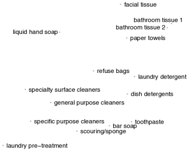
shopper provides a better predictive model of consumer behavior. We now use the fitted model to qualitatively understand the data.

First, we assess the attributes vectors $\alpha_{c}$ , confirming that they capture meaningful dimensions of the items. (Recall that each is a 100-dimensional real-valued vector.) As one demonstration, we project them on to 2-dimensional space using t-distributed stochastic neighbor embedding (t-sne) (van der Maaten and Hinton, 2008), and then examine the items in different regions of the projected space. Figure 3 shows two particular regions: one collects different types of pet food and supplies; the other collects different cleaning products. As a second demonstration, we can use the cosine distance to find similar items similar to a “query item.” Table 6 shows the top-three most similar items to a set of queries.

mollusks	organic vegetables	granulated sugar	cat food dry/moist
finfish all other - frozen	organic fruits	flour	cat food wet
crustacean non-shrimp	citrus	baking ingredients	cat litter & deodorant
shrimp family	cooking vegetables	brown sugar	pet supplies

Table 6: Most similar items to a query item (given in the first row), according to the cosine distance between the item features

\alpha_{c}

, for the category-level experiment.

Halloween candy		cherries		turkey - frozen
$3.46$	$2006/10/25$	$3.07$	$2006/06/28$	$3.56$	$2005/11/16$
$3.34$	$2005/10/26$	$3.01$	$2006/07/12$	$3.30$	$2006/11/15$
$2.81$	$2005/10/19$	$2.85$	$2006/06/21$	$2.64$	$2005/11/23$
			$\vdots$
$-1.28$	$2005/11/23$	$-3.59$	$2006/10/11$	$-1.25$	$2006/06/21$
$-1.31$	$2007/01/03$	$-3.89$	$2006/10/18$	$-1.29$	$2006/07/05$
$-1.33$	$2005/11/16$	$-4.54$	$2006/10/25$	$-1.30$	$2006/07/19$

Table 7: Highest and lowest seasonal effects, as given by

\mu_{c}^{\top}\delta_{w}

, for three example items. The model finds the effects of holidays such as Halloween or Thanksgiving, as well as the seasonal availability of fruits.

Other latent variables reveal different aspects of consumer behavior. For example, Table 7 show the highest and lowest seasonal effects for a set of items. The model correctly captures how Haloween candy is more popular near Halloween; and turkey is more popular near Thanksgiving. It also captures the seasonal availability of fruits, e.g., cherries.

These investigations are on the category-level analysis. For more fine-grained qualitative assessments—especially those around complementarity and exchangeability—we now turn to the upc-level model.

6.2 UPC-level data

We fit shopper to upc-level data, which contains $5$ , $590$ unique items. We use the same dimensionality of the latent vectors as in Section 6.1, i.e., $K=100$ for $\alpha_{c}$ , $\rho_{c}$ , and $\theta_{u}$ , and $10$ latent features for the seasonal and price vectors. We additionally tie the price vectors $\beta_{c}$ and seasonal effect vectors $\delta_{c}$ to all items in the same category. To speed up computation, we fit this model without thinking ahead.

We can again find similar items to “query” items using the cosine distance between attribute vectors $\alpha_{c}$ . Table 8 shows similar items for several queries; the model identifies qualitatively related items.

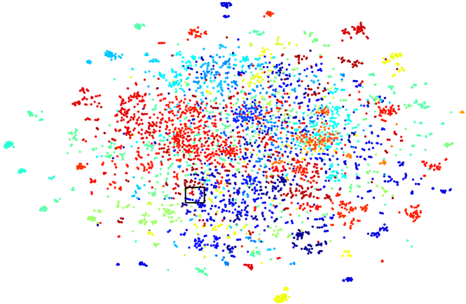
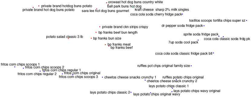
For another view, Figure 4 shows a two-dimensional t-sne projection (van der Maaten and Hinton, 2008) of the attribute vectors. This figure colors the items according to their group, and it reveals that items in the same category are often close to each other in attribute space. (Groups are defined as one level of hierarchy above categories; some examples are “jams, jellies, and spreads,” “salty snacks,” or “canned fruits.”) When groups are mixed in a region, they tend to be items that appear in similar contexts, e.g., hot dogs, hamburger buns, and soda (Figure 5).

Dentyne ice gum peppermint	california avocados	Coca Cola classic soda fridge pack 1
Wrigleys gum orbit white peppermint	tomatoes red tov/cluster	Sprite soda fridge pack
Dentyne ice shivermint	apples fuji medium 100ct	Coca Cola classic fridge pack 2
Dentyne ice gum spearmint	tomatoes roma red	Coca Cola soda cherry fridge pack

Table 8: Most similar items to a query item (given in the first row), according to the cosine distance between the item features

\alpha_{c}

, for the upc-level experiment.

6.2.1 Substitutes, complements, and exchangeability metrics

A key objective for applications of shopper is to be able to estimate interaction effects among products. These effects are described by the coefficients $\rho_{c}$ and attributes $\alpha_{c}$ . When $\rho_{c}^{\top}\alpha_{c^{\prime}}$ and $\rho_{c^{\prime}}^{\top}\alpha_{c}$ are large, this means that purchasing item $c^{\prime}$ increases the consumer’s preference for $c$ , and vice-versa. When these two terms are negative and large, the items may be substitutes—putting one item in the basket reduces the need for the other item.

All else equal, complements are relatively likely to be purchased together, while substitutes are less likely to be purchased together. In addition, for complementary items $c$ and $c^{\prime}$ , when the price of $c^{\prime}$ increases, the customer is less likely to purchase item $c$ . We define the complementarity metric as

\displaystyle C_{cc^{\prime}}\triangleq\frac{1}{2}\left(\rho_{c}^{\top}\alpha_{c^{\prime}}+\rho_{c^{\prime}}^{\top}\alpha_{c}\right).

(12)

Most shopping data is sparse—each individual item has a low probability of purchase—and so it can be difficult to accurately identify pairs of items that are substitutes. We introduce a new metric, which we call exchangeability, that can help identify substitutes. For a pair of items $(c,c^{\prime})$ , our notion of exchangeability depends on the distributions of items that are induced when conditioning on $c$ or $c^{\prime}$ ; if those distributions are similar then we say that $c$ and $c^{\prime}$ are exchangeable.

Let $p_{k|c}$ denote the probability of item $k$ given that item $c$ is the only item in the basket (in this definition, we zero-out the probabilities of items $c$ , $c^{\prime}$ , and checkout). We measure the similarity between the distributions $p_{\cdot|c}$ and $p_{\cdot|c^{\prime}}$ with symmetrized kl divergence. The exchangeability metric is

	$\displaystyle E_{cc^{\prime}}$	$\displaystyle\triangleq\frac{1}{2}\left(D_{\textrm{KL}}\left(p_{\cdot\|c}\;\|\|\;p_{\cdot\|c^{\prime}}\right)+D_{\textrm{KL}}\left(p_{\cdot\|c^{\prime}}\;\|\|\;p_{\cdot\|c}\right)\right)$		(13)
		$\displaystyle=\frac{1}{2}\sum_{k\neq c,c^{\prime}}\left(p_{k\|c}\log\frac{p_{k\|c}}{p_{k\|c^{\prime}}}+p_{k\|c^{\prime}}\log\frac{p_{k\|c^{\prime}}}{p_{k\|c}}\right).$

With this definition, two items that are intuitively exchangeable—such as two different prepared sandwiches, or two yogurts that are the same brand—will exhibit smaller values of $E_{cc^{\prime}}$ .

With several example queries, Table 9 shows the three most complementary items and the three most exchangeable items. In the computation of the probabilities $p_{k|c}$ , we consider an “average customer” (obtained by averaging the per-user vectors) in an “average week” (obtained by averaging the per-week vectors). The probabilities were also obtained assuming that no other item except $c$ is in the shopping basket. shopper correctly recovers complements, such as taco shells and taco seasoning, hot dogs and buns, and mustard and hamburger buns. shopper typically identifies the most exchangeable items as being of the same type, such as several types of buns or tortillas; highly exchangeable items are suggestive of substitutes.

Finally, note that shopper can model triplets of complementary items when they are also pairwise complements, but it cannot in cases where the triplets do not form complementary pairs.

query items	complementarity score		exchangeability score
mission tortilla soft taco 1	$2.40$	taco bell taco seasoning mix	$0.05$	mission fajita size
	$2.26$	mcrmck seasoning mix taco	$0.07$	mission tortilla soft taco 2
	$2.24$	lawrys taco seasoning mix	$0.13$	mission tortilla fluffy gordita
private brand hot dog buns	$2.99$	bp franks meat	$0.11$	ball park buns hot dog
	$2.63$	bp franks bun size	$0.13$	private brand hotdog buns potato 1
	$2.37$	bp franks beed bun length	$0.15$	private brand hotdog buns potato 2
private brand mustard squeeze bottle	$0.50$	private brand hot dog buns	$0.15$	frenchs mustard classic yellow squeeze
	$0.41$	private brand cutlery full size forks	$0.16$	frenchs mustard classic yellow squeezed
	$0.24$	best foods mayonnaise squeeze	$0.21$	heinz ketchup squeeze bottle
private brand napkins all occasion	$0.78$	private brand selection plates 6 7/8 in	$0.09$	vnty fair napkins all occasion 1
	$0.50$	private brand selection plates 8 3/4 in	$0.11$	vnty fair napkins all occasion 2
	$0.49$	private brand cutlery full size forks	$0.12$	private brand selection premium napkins

Table 9: Items with the highest complementarity and lowest exchangeability metrics for some query items.

7 Discussion

We developed shopper, a probabilistic model of consumer behavior. shopper is a sequential model of a consumer that posits a latent structure to how he or she shops. In posterior inference, shopper estimates item attributes, item-item interactions, price elasticities, seasonal effects, and customer preferences. We used shopper to analyze large-scale shopping data from a grocery store and evaluated it with out-of-sample predictions. In addition to evaluating on a random sample of held out data, we also evaluated on counterfactual test sets, i.e., on days where prices are systematically different from average.

shopper is a computationally feasible, interpretable approach to modeling consumer choice over complex shopping baskets. While the existing literature in economics and marketing usually considers two or three products (Berry et al., 2014), shopper enables considering choices among thousands of products that potentially interact with one another. Using supermarket shopping data, we show that shopper can uncover these relationships.

There are several avenues for future work. Consider the question of how the probabilistic model relates to maximizing a consumer’s utility of the entire basket. Section 2.1.2 introduced a heuristic model of consumer behavior that is consistent with the probabilistic model. This heuristic lends itself to computational tractability; it enables us to analyze datasets of baskets that involve thousands of products and thousands of consumers. But the heuristic also involves a fairly myopic consumer. In future work, it is interesting to consider alternative heuristic models.

Another avenue is to embellish the distribution of baskets. One way is to expand the model to capture within-basket heterogeneity. Shopping trips may reflect a collection of needs, such as school lunches, a dinner party, and pet care, and items may interact with other items within each need. Capturing the heterogenous patterns within the baskets would sharpen the estimated interactions. Another embellishment is to expand the model of baskets to include a budget. A budget imposes constraints on the number of items (or their total price) purchased in a single trip.

Acknowledgements

Francisco J. R. Ruiz is supported by the EU H2020 programme (Marie Skłodowska-Curie Individual Fellowship, grant agreement 706760). This work is also supported by ONR N00014-17-1-2131, NIH 1U01MH115727-01, DARPA SD2 FA8750-18-C-0130, ONR N00014-15-1-2209, NSF CCF-1740833, IBM, 2Sigma, and Amazon. The authors also thank Tilman Drerup and Tobias Schmidt for research assistance, the seminar participants at Stanford, as well as the Cyber Initiative at Stanford. Finally, we also acknowledge the support of NVIDIA Corporation with the donation of a GPU used for this research.

Appendix A Details on the Inference Algorithm

Here we provide the technical details of the variational inference procedure and a description of the full algorithm.

Recall the notation introduced in Section 5 of the main paper, where $\boldsymbol{\mathbf{\ell}}=\{\rho,\alpha,\lambda,\theta,\gamma,\beta,\mu,\delta\}$ denotes the set of all latent variables in the model, $\mathpzc{y}=\{\mathpzc{y}_{t}\}$ is the collection of (unordered) baskets, and $x=x_{1:T}$ , where $x_{t}=(u_{t},w_{t},r_{t})$ are observed covariates of the shopping trips. We use mean-field variational inference, i.e., we approximate the posterior $p(\boldsymbol{\mathbf{\ell}}\,|\,\mathpzc{y},\mathbf{x})$ with a fully factorized variational distribution,

\begin{split}q(\boldsymbol{\mathbf{\ell}})=&\prod_{c}q(\alpha_{c})q(\rho_{c})q(\lambda_{c})q(\beta_{c})q(\mu_{c})\times\prod_{u}q(\theta_{u})q(\gamma_{u})\times\prod_{w}q(\delta_{w}).\end{split}

(14)

We set each variational factor in the same family as the prior, i.e., Gaussian variational distributions with diagonal covariance matrices for $q(\rho_{i})$ , $q(\alpha_{i})$ , $q(\lambda_{i})$ , $q(\nu_{u})$ , $q(\mu_{i})$ , and $q(\delta_{w})$ , and independent gamma variational distributions for the price sensitivity terms $q(\gamma_{u})$ and $q(\beta_{i})$ . We parameterize the Gaussian in terms of its mean and standard deviation, and we parameterize the gamma in terms of its shape and mean.

Let $\nu$ denote the vector containing all the variational parameters. We wish to find the variational parameters $\nu$ that maximize the elbo,

\begin{split}\mathcal{L}(\nu)&=\mathbb{E}_{q(\boldsymbol{\mathbf{\ell}}\,;\,\nu)}\left[\log p(\mathpzc{y}\,|\,\mathbf{x},\boldsymbol{\mathbf{\ell}})+\log p(\boldsymbol{\mathbf{\ell}})-\log q(\boldsymbol{\mathbf{\ell}}\,;\,\nu)\right]\\ &=\mathbb{E}_{q(\boldsymbol{\mathbf{\ell}}\,;\,\nu)}\left[\sum_{t=1}^{T}\log p(\mathpzc{y}_{t}\,|\,x_{t},\boldsymbol{\mathbf{\ell}})+\log p(\boldsymbol{\mathbf{\ell}})-\log q(\boldsymbol{\mathbf{\ell}}\,;\,\nu)\right]\\ &\leq\log p(\mathpzc{y}\,|\,\mathbf{x}).\end{split}

(15)

In this supplement, we show how to apply stochastic optimization to maximize the bound on the log marginal likelihood. More in detail, we first describe how to tackle the intractable expectations using stochastic optimization and the reparameterization trick, and then we show how to leverage stochastic optimization to decrease the computational complexity.

A.1 Intractable expectations: Stochastic optimization and the reparameterization trick

We are interested in maximizing an objective function of the form

\widetilde{\mathcal{L}}(\nu)=\mathbb{E}_{q(\boldsymbol{\mathbf{\ell}}\,;\,\nu)}\left[f(\boldsymbol{\mathbf{\ell}},\nu)\right]

(16)

with respect to the parameters $\nu$ . In the particular case that $f(\boldsymbol{\mathbf{\ell}},\nu)=\log p(\mathpzc{y},\boldsymbol{\mathbf{\ell}}\,|\,\mathbf{x})-\log q(\boldsymbol{\mathbf{\ell}}\,;\,\nu)$ , we recover the elbo in Eq. 15, but we prefer to keep the notation general because in Section A.2 we will consider other functions $f(\boldsymbol{\mathbf{\ell}},\nu)$ .

The main challenge is that the expectations in Eq. 16 are analytically intractable. Thus, the variational algorithm we develop aims at obtaining and following noisy estimates of the gradient $\nabla_{\nu}\widetilde{\mathcal{L}}$ . We obtain these estimates via stochastic optimization; in particular, we apply the reparameterization trick to form Monte Carlo estimates of the gradient (Kingma and Welling, 2014; Titsias and Lázaro-Gredilla, 2014; Rezende, Mohamed and Wierstra, 2014).

In reparameterization, we first introduce a transformation of the latent variables $\boldsymbol{\mathbf{\ell}}=\mathcal{T}(\boldsymbol{\epsilon}\,;\,\nu)$ and an auxiliary distribution $\pi(\boldsymbol{\epsilon}\,;\,\nu)$ , such that we can obtain samples from the variational distribution $q(\boldsymbol{\mathbf{\ell}}\,;\,\nu)$ following a two-step process:

\boldsymbol{\epsilon}\sim\pi(\boldsymbol{\epsilon}\,;\,\nu),\qquad\boldsymbol{\mathbf{\ell}}=\mathcal{T}(\boldsymbol{\epsilon}\,;\,\nu).

(17)

The requirement for $\pi(\boldsymbol{\epsilon}\,;\,\nu)$ and $\mathcal{T}(\boldsymbol{\epsilon}\,;\,\nu)$ is that this procedure must provide a variable $\boldsymbol{\mathbf{\ell}}$ that is distributed according to $\boldsymbol{\mathbf{\ell}}\sim q(\boldsymbol{\mathbf{\ell}}\,;\,\nu)$ . Here we have considered the generalized reparameterization approach (Ruiz, Titsias and Blei, 2016; Naesseth et al., 2017), which allows the auxiliary distribution $\pi(\boldsymbol{\epsilon}\,;\,\nu)$ to depend on the variational parameters $\nu$ (this is necessary because the gamma random variables are not otherwise reparameterizable).

Once we have introduced the auxiliary variable $\boldsymbol{\epsilon}$ , we can rewrite the gradient of the objective in Eq. 16 as an expectation with respect to the auxiliary distribution $\pi(\boldsymbol{\epsilon}\,;\,\nu)$ ,

\nabla_{\nu}\widetilde{\mathcal{L}}=\nabla_{\nu}\mathbb{E}_{q(\boldsymbol{\mathbf{\ell}}\,;\,\nu)}\left[f(\boldsymbol{\mathbf{\ell}},\nu)\right]=\nabla_{\nu}\mathbb{E}_{\pi(\boldsymbol{\epsilon}\,;\,\nu)}\left[f\left(\mathcal{T}(\boldsymbol{\epsilon}\,;\,\nu),\nu\right)\right].

(18)

We now push the gradient into the integral¹¹1In the model that includes thinking-ahead, this step introduces a small bias due to the non-differentiability of the $\max(\cdot)$ operator; see Lee, Yu and Yang (2018). and apply the chain rule for derivatives to express the gradient as an expectation,

\begin{split}\nabla_{\nu}\widetilde{\mathcal{L}}=\mathbb{E}_{\pi(\boldsymbol{\epsilon}\,;\,\nu)}\left[\nabla_{\boldsymbol{\mathbf{\ell}}}f(\boldsymbol{\mathbf{\ell}},\nu)\big{|}_{\boldsymbol{\mathbf{\ell}}=\mathcal{T}(\boldsymbol{\epsilon}\,;\,\nu)}\nabla_{\nu}\mathcal{T}(\boldsymbol{\epsilon}\,;\,\nu)+f\left(\mathcal{T}(\boldsymbol{\epsilon}\,;\,\nu),\nu\right)\nabla_{\nu}\log\pi(\boldsymbol{\epsilon}\,;\,\nu)\right].\end{split}

(19)

To obtain this expression, we have assumed that $\mathbb{E}_{\pi(\boldsymbol{\epsilon}\,;\,\nu)}\left[\nabla_{\nu}f(\boldsymbol{\mathbf{\ell}},\nu)\big{|}_{\boldsymbol{\mathbf{\ell}}=\mathcal{T}(\boldsymbol{\epsilon}\,;\,\nu)}\right]=0$ because the only dependence of $f(\boldsymbol{\mathbf{\ell}},\nu)$ on $\nu$ is through the term $\log q(\boldsymbol{\mathbf{\ell}}\,;\,\nu)$ , and the expectation of the score function is zero.

We can now obtain a Monte Carlo estimate of the expectation in Eq. 19 (and therefore of the gradient of interest) by drawing a sample from $\pi(\boldsymbol{\epsilon}\,;\,\nu)$ and evaluating the argument of the expectation. That is, we form the gradient estimator as

\begin{split}\widehat{\nabla}_{\nu}\widetilde{\mathcal{L}}=\nabla_{\boldsymbol{\mathbf{\ell}}}f(\boldsymbol{\mathbf{\ell}},\nu)\big{|}_{\boldsymbol{\mathbf{\ell}}=\mathcal{T}(\boldsymbol{\epsilon}\,;\,\nu)}\nabla_{\nu}\mathcal{T}(\boldsymbol{\epsilon}\,;\,\nu)+f\left(\mathcal{T}(\boldsymbol{\epsilon}\,;\,\nu),\nu\right)\nabla_{\nu}\log\pi(\boldsymbol{\epsilon}\,;\,\nu),\end{split}

(20)

where $\boldsymbol{\epsilon}\sim\pi(\boldsymbol{\epsilon}\,;\,\nu)$ . This assumes that we are able to evaluate $f(\boldsymbol{\mathbf{\ell}},\nu)$ and its gradient. (We show in Section A.2 how to do that efficiently.)

We use a transformation $\mathcal{T}(\cdot)$ and auxiliary distribution $\pi(\cdot)$ for each variational factor. For a Gaussian variational factor with mean $\mu$ and standard deviation $\sigma$ , we use the standard reparameterization,

\mathcal{T}_{\textrm{Gauss}}(\varepsilon\,;\,\mu,\sigma)=\mu+\sigma\varepsilon,\qquad\pi_{\textrm{Gauss}}(\varepsilon\,;\,\mu,\sigma)=\mathcal{N}(0,1),

(21)

which makes the last term of Eq. 20 vanish because $\nabla_{\nu}\log\pi_{\textrm{Gauss}}(\varepsilon\,;\,\mu,\sigma)=0$ . For a gamma variational factor with shape $\alpha$ and mean $\mu$ , we use the transformation based on rejection sampling (Marsaglia and Tang, 2000),

\mathcal{T}_{\textrm{Gamma}}(\varepsilon\,;\,\alpha,\mu)=\frac{\mu}{\alpha}\left(\alpha-\frac{1}{3}\right)\left(1+\frac{\varepsilon}{\sqrt{9\alpha-3}}\right)^{3},

(22)

and $\pi_{\textrm{Gamma}}(\varepsilon\,;\,\alpha,\mu)$ is defined though a rejection sampling procedure. See Naesseth et al. (2017) for further details about the reparameterization trick for gamma random variables.²²2In particular, we also apply the “shape augmentation trick,” which allows us to reparameterize a gamma random variable with shape $\alpha$ in terms of another gamma random variable with shape $\alpha+P$ , where $P$ is a positive integer. We use $P=10$ . See Naesseth et al. (2017) for additional details.

Algorithm 1 summarizes the resulting variational inference procedure. At each iteration, we obtain a sample from $\boldsymbol{\mathbf{\ell}}$ via the auxiliary distribution $\pi(\boldsymbol{\epsilon}\,;\,\nu)$ and the transformation $\mathcal{T}(\boldsymbol{\epsilon}\,;\,\nu)$ ; we evaluate the function $f(\boldsymbol{\mathbf{\ell}},\nu)$ and its gradient with respect to the latent variables $\boldsymbol{\mathbf{\ell}}$ ; we obtain the gradient estimate in Eq. 20; and we take a gradient step for the variational parameters $\nu$ . In the stochastic optimization procedure, we adaptively set the step size as proposed in the automatic differentiation variational inference (advi) algorithm (Kucukelbir et al., 2017).

input : Data

\mathpzc{y}

and

x

, model hyperparameters

output : Variational parameters

\nu

Initialize

\nu

randomly

Initialize iteration number

m\leftarrow 1

repeat

Sample

\boldsymbol{\epsilon}\sim\pi(\boldsymbol{\epsilon}\,;\,\nu)

Compute

\boldsymbol{\mathbf{\ell}}=\mathcal{T}(\boldsymbol{\epsilon}\,;\,\nu)

Evaluate

f(\boldsymbol{\mathbf{\ell}},\nu)

and

\nabla_{\boldsymbol{\mathbf{\ell}}}f(\boldsymbol{\mathbf{\ell}},\nu)

(see Algorithm 2)

Obtain an estimate of the gradient,

\widehat{\nabla}_{\nu}\widetilde{\mathcal{L}}

(Eq. 20)

Set the step size

\eta^{(m)}

(e.g., use the schedule proposed in advi)

Take a gradient step,

\nu\leftarrow\nu+\eta^{(m)}\odot\widehat{\nabla}_{\nu}\widetilde{\mathcal{L}}

Increase the iteration number,

m\leftarrow m+1

until convergence

return

\nu

Algorithm 1 Variational inference algorithm

A.2 Computational complexity: Stochastic optimization and lower bounds

The algorithm in Section A.1 requires to evaluate the model log joint (as well as its gradient). There are three issues that make it expensive to evaluate the log joint. First, evaluating the log likelihood is expensive because it involves a summation over shopping trips. This represents a problem when the dataset is large. Second, evaluating the softmax involves computing its normalization constant, which contains a summation over all items. This becomes an issue when there are thousands of items and we need to evaluate many softmax probabilities. Third, computing the probability over unordered baskets $\mathpzc{y}_{t}$ is also expensive, as it involves a summation over all possible permutations.

We address these issues by combining two techniques: data subsampling and lower bounds on the elbo. We first describe data subsampling for evaluating the log likelihood. Note that the log likelihood involves a summation over many terms,

\log p(\mathpzc{y}\,|\,\mathbf{x},\boldsymbol{\mathbf{\ell}})=\sum_{t=1}^{T}\log p(\mathpzc{y}_{t}\,|\,x_{t},\boldsymbol{\mathbf{\ell}}).

(23)

We can obtain an unbiased estimate of the log likelihood (and its gradient) by sampling a random subset of shopping trips. Let $\mathcal{B}_{T}$ be the (randomly chosen) set of trips. The estimator

\frac{T}{|\mathcal{B}_{T}|}\sum_{t\in\mathcal{B}_{T}}\log p(\mathpzc{y}_{t}\,|\,x_{t},\boldsymbol{\mathbf{\ell}})

is unbiased because its expected value is the log likelihood $\log p(\mathpzc{y}\,|\,\mathbf{x},\boldsymbol{\mathbf{\ell}})$ (Hoffman et al., 2013). Thus, we subsample data terms to obtain unbiased estimates of the log likelihood and its gradient, resulting in a computationally more efficient algorithm.

Second, we describe how to form variational bounds to address the issue of the expensive normalization constant of the softmax. Each softmax log probability is given by

\log p(y_{ti}=c\,|\,\boldsymbol{\mathbf{y}}_{t,i-1})=\Psi(c,\boldsymbol{\mathbf{y}}_{t,i-1})-\log\left(\sum_{c^{\prime}\notin\boldsymbol{\mathbf{y}}_{t,i-1}}\exp\{\Psi(c^{\prime},\boldsymbol{\mathbf{y}}_{t,i-1})\}\right).

(24)

The summation over $c^{\prime}$ is expensive, and we cannot easily form an unbiased estimator because of the non-linearity introduced by the logarithm. Hence, we apply the one-vs-each bound (Titsias, 2016), which allows us to write

\log p(y_{ti}=c\,|\,\boldsymbol{\mathbf{y}}_{t,i-1})\geq\sum_{c^{\prime}\notin[\boldsymbol{\mathbf{y}}_{t,i-1},c]}\log\sigma\big{(}\Psi(c,\boldsymbol{\mathbf{y}}_{t,i-1})-\Psi(c^{\prime},\boldsymbol{\mathbf{y}}_{t,i-1})\big{)},

(25)

where $\sigma(x)=\frac{1}{1+e^{-x}}$ is the sigmoid function. We can form unbiased estimates of the summation via subsampling. More precisely, we randomly sample a set $\mathcal{B}_{C}^{(t,i)}$ of items (each of them distinct from $c$ and from the other items in the basket). Then, we form the following unbiased estimator:

\frac{C-i}{|\mathcal{B}_{C}^{(t,i)}|}\sum_{c^{\prime}\in\mathcal{B}_{C}^{(t,i)}}\log\sigma\big{(}\Psi(c,\boldsymbol{\mathbf{y}}_{t,i-1})-\Psi(c^{\prime},\boldsymbol{\mathbf{y}}_{t,i-1})\big{)}.

Here, $C$ stands for the total number of items.

Finally, we show how to deal with the issue of unordered baskets. Recall that each log likelihood term involves a summation over all possible permutations of the baskets (holding the checkout item in the last position),

\log p(\mathpzc{y}_{t}\,|\,x_{t},\boldsymbol{\mathbf{\ell}})=\log\left(\sum_{\pi_{t}}p(\boldsymbol{\mathbf{y}}_{t,\pi_{t}}\,|\,x_{t},\boldsymbol{\mathbf{\ell}})\right).

(26)

Following a similar procedure as Doshi-Velez et al. (2009), we introduce an auxiliary distribution $q(\pi_{t})$ to rewrite the expression above as an expectation with respect to $q(\pi_{t})$ , and then we apply Jensen’s inequality:

\begin{split}\log p(\mathpzc{y}_{t}\,|\,x_{t},\boldsymbol{\mathbf{\ell}})&=\log\left(\mathbb{E}_{q(\pi_{t})}\left[\frac{p(\boldsymbol{\mathbf{y}}_{t,\pi_{t}}\,|\,x_{t},\boldsymbol{\mathbf{\ell}})}{q(\pi_{t})}\right]\right)\\ &\geq\mathbb{E}_{q(\pi_{t})}\left[\log p(\boldsymbol{\mathbf{y}}_{t,\pi_{t}}\,|\,x_{t},\boldsymbol{\mathbf{\ell}})-\log q(\pi_{t})\right]\\ &=\sum_{\pi_{t}}q(\pi_{t})\left(\log p(\boldsymbol{\mathbf{y}}_{t,\pi_{t}}\,|\,x_{t},\boldsymbol{\mathbf{\ell}})-\log q(\pi_{t})\right).\end{split}

(27)

Since the bound involves a direct summation over permutations, we can subsample terms to alleviate the computational complexity. For simplicity, we set $q(\pi_{t})$ to be a uniform distribution over all possible permutations, and thus we do not introduce auxiliary variational parameters that would be too expensive to obtain otherwise. In particular, we form an unbiased estimate of the bound by sampling one random permutation $\pi_{t}$ and evaluating the term³³3We ignore the term $\log q(\pi_{t})$ because it is a constant.

\log p(\boldsymbol{\mathbf{y}}_{t,\pi_{t}}\,|\,x_{t},\boldsymbol{\mathbf{\ell}}).

To sum up, we have derived a bound of the elbo,

\widetilde{\mathcal{L}}(\nu)\leq\mathcal{L}(\nu)\leq\log p(\mathpzc{y}\,|\,x),

(28)

which can still be written as an expectation with respect to the variational distribution $q(\boldsymbol{\mathbf{\ell}}\,|\,\nu)$ . More importantly, we can efficiently evaluate the argument $f(\boldsymbol{\mathbf{\ell}},\nu)$ of such expectation and its gradient with respect to the latent variables $\boldsymbol{\mathbf{\ell}}$ .

Putting all together, the function $f(\boldsymbol{\mathbf{\ell}},\nu)$ that we use is given by

\begin{split}f(\boldsymbol{\mathbf{\ell}},\nu)=&\sum_{t=1}^{T}\sum_{\pi_{t}}q(\pi_{t})\sum_{i=1}^{n_{t}}\sum_{c^{\prime}\notin[\boldsymbol{\mathbf{y}}_{t,i-1},c]}\log\sigma\big{(}\Psi(c,\boldsymbol{\mathbf{y}}_{t,i-1})-\Psi(c^{\prime},\boldsymbol{\mathbf{y}}_{t,i-1})\big{)}\\ &+\log p(\boldsymbol{\mathbf{\ell}})-\log q(\boldsymbol{\mathbf{\ell}}\,;\,\nu).\end{split}

(29)

We obtain an unbiased estimate via subsampling shopping trips, one permutation $\pi_{t}$ for each one, and items $c^{\prime}$ . We use $|\mathcal{B}_{T}|=100$ trips and $|\mathcal{B}_{C}^{(t,i)}|=50$ items in our experiments.

input : Data

\mathpzc{y}

and

x

, a sample of the latent parameters

\boldsymbol{\mathbf{\ell}}

, variational distribution

q(\boldsymbol{\mathbf{\ell}}\,;\,\nu)

output : An unbiased estimate of

f(\boldsymbol{\mathbf{\ell}},\nu)

and its gradient (for the gradient, differentiate through the algorithm)

Initialize

\widehat{f}\leftarrow\log p(\boldsymbol{\mathbf{\ell}})-\log q(\boldsymbol{\mathbf{\ell}}\,;\,\nu)

Sample a set of baskets

\mathcal{B}_{T}\subseteq\{1,\ldots,T\}

for $t\in\mathcal{B}_{T}$ do

Sample a permutation

\pi_{t}

of the items in basket

t

Set

\boldsymbol{\mathbf{y}}_{t}

to the vector containing the items in basket

t

ordered according to

\pi_{t}

for $i=1,\ldots,n_{t}$ do

Set

c

to the

i

th item in

\boldsymbol{\mathbf{y}}_{t}

Sample a set of items

\mathcal{B}_{C}^{(t,i)}\subseteq\{1,\ldots,C\}\diagdown\{\boldsymbol{\mathbf{y}}_{t,i-1},c\}

for $c^{\prime}\in\mathcal{B}_{C}^{(t,i)}$ do

Update

\widehat{f}\leftarrow\widehat{f}+\frac{T}{|\mathcal{B}_{T}|}\times\frac{C-i}{|\mathcal{B}_{C}^{(t,i)}|}\times\log\sigma\big{(}\Psi(c,\boldsymbol{\mathbf{y}}_{t,i-1})-\Psi(c^{\prime},\boldsymbol{\mathbf{y}}_{t,i-1})\big{)}

end for

return

\widehat{f}

and

\nabla_{\boldsymbol{\mathbf{\ell}}}\widehat{f}

Algorithm 2 Estimate of

f(\boldsymbol{\mathbf{\ell}},\nu)

(Eq. 29)

Algorithm 2 outlines the procedure to obtain an unbiased estimate of $f(\boldsymbol{\mathbf{\ell}},\nu)$ for a given sample of the latent parameters, $\boldsymbol{\mathbf{\ell}}\sim q(\boldsymbol{\mathbf{\ell}}\,;\,\nu)$ . Differentiation though Algorithm 2 gives the gradient $\nabla_{\boldsymbol{\mathbf{\ell}}}f(\boldsymbol{\mathbf{\ell}},\nu)$ , which is also required in the inference procedure (Algorithm 1).

References

Abernethy et al. (2009) {barticle}[author] \bauthor\bsnmAbernethy, \bfnmJ.\binitsJ., \bauthor\bsnmBach, \bfnmF.\binitsF., \bauthor\bsnmEvgeniou, \bfnmT.\binitsT. and \bauthor\bsnmVert, \bfnmJ. P.\binitsJ. P. (\byear2009). \btitleA New Approach to Collaborative Filtering: Operator Estimation with Spectral Regularization. \bjournalJournal of Machine Learning Research \bvolume10 \bpages803–826. \endbibitem
Arora et al. (2016) {barticle}[author] \bauthor\bsnmArora, \bfnmS.\binitsS., \bauthor\bsnmLi, \bfnmY.\binitsY., \bauthor\bsnmLiang, \bfnmY.\binitsY. and \bauthor\bsnmMa, \bfnmT.\binitsT. (\byear2016). \btitleRAND-WALK: A latent variable model approach to word embeddings. \bjournalTransactions of the Association for Computational Linguistics \bvolume4. \endbibitem
Athey and Stern (1998) {btechreport}[author] \bauthor\bsnmAthey, \bfnmSusan\binitsS. and \bauthor\bsnmStern, \bfnmScott\binitsS. (\byear1998). \btitleAn empirical framework for testing theories about complimentarity in organizational design \btypeTechnical Report, \bpublisherNational Bureau of Economic Research. \endbibitem
Bamler and Mandt (2017) {binproceedings}[author] \bauthor\bsnmBamler, \bfnmR.\binitsR. and \bauthor\bsnmMandt, \bfnmS.\binitsS. (\byear2017). \btitleDynamic word embeddings via skip-gram filtering. In \bbooktitleInternational Conference in Machine Learning. \endbibitem
Barkan (2016) {barticle}[author] \bauthor\bsnmBarkan, \bfnmO.\binitsO. (\byear2016). \btitleBayesian neural word embedding. \bjournalarXiv preprint arXiv:1603.06571. \endbibitem
Barkan and Koenigstein (2016) {binproceedings}[author] \bauthor\bsnmBarkan, \bfnmO.\binitsO. and \bauthor\bsnmKoenigstein, \bfnmN.\binitsN. (\byear2016). \btitleItem2Vec: Neural item embedding for collaborative filtering. In \bbooktitleIEEE International Workshop on Machine Learning for Signal Processing. \endbibitem
Bengio et al. (2003) {barticle}[author] \bauthor\bsnmBengio, \bfnmY.\binitsY., \bauthor\bsnmDucharme, \bfnmR.\binitsR., \bauthor\bsnmVincent, \bfnmP.\binitsP. and \bauthor\bsnmJanvin, \bfnmC.\binitsC. (\byear2003). \btitleA Neural Probabilistic Language Model. \bjournalJournal of Machine Learning Research \bvolume3 \bpages1137–1155. \endbibitem
Bengio et al. (2006) {bincollection}[author] \bauthor\bsnmBengio, \bfnmY.\binitsY., \bauthor\bsnmSchwenk, \bfnmH.\binitsH., \bauthor\bsnmSenécal, \bfnmJ. S.\binitsJ. S., \bauthor\bsnmMorin, \bfnmF.\binitsF. and \bauthor\bsnmGauvain, \bfnmJ. L.\binitsJ. L. (\byear2006). \btitleNeural probabilistic language models. In \bbooktitleInnovations in Machine Learning \bpublisherSpringer. \endbibitem
Berry et al. (2014) {barticle}[author] \bauthor\bsnmBerry, \bfnmSteven\binitsS., \bauthor\bsnmKhwaja, \bfnmAhmed\binitsA., \bauthor\bsnmKumar, \bfnmVineet\binitsV., \bauthor\bsnmMusalem, \bfnmAndres\binitsA., \bauthor\bsnmWilbur, \bfnmKenneth C\binitsK. C., \bauthor\bsnmAllenby, \bfnmGreg M\binitsG. M., \bauthor\bsnmAnand, \bfnmBharat N\binitsB. N., \bauthor\bsnmChintagunta, \bfnmPradeep K\binitsP. K., \bauthor\bsnmHanemann, \bfnmW Michael\binitsW. M., \bauthor\bsnmJeziorski, \bfnmPrzemyslaw\binitsP. \betalet al. (\byear2014). \btitleStructural models of complementary choices. \bjournalMarketing Letters \bvolume25 \bpages245–256. \endbibitem
Blei, Kucukelbir and McAuliffe (2017) {barticle}[author] \bauthor\bsnmBlei, \bfnmD. M.\binitsD. M., \bauthor\bsnmKucukelbir, \bfnmA.\binitsA. and \bauthor\bsnmMcAuliffe, \bfnmJ. D.\binitsJ. D. (\byear2017). \btitleVariational Inference: A Review for Statisticians. \bjournalJournal of the American Statistical Association \bvolume112 \bpages859–877. \endbibitem
Blum (1954) {barticle}[author] \bauthor\bsnmBlum, \bfnmJ. R.\binitsJ. R. (\byear1954). \btitleApproximation methods which converge with probability one. \bjournalThe Annals of Mathematical Statistics \bvolume25 \bpages382–386. \endbibitem
Bottou, Curtis and Nocedal (2016) {barticle}[author] \bauthor\bsnmBottou, \bfnmLéon\binitsL., \bauthor\bsnmCurtis, \bfnmFrank E.\binitsF. E. and \bauthor\bsnmNocedal, \bfnmJorge\binitsJ. (\byear2016). \btitleOptimization Methods for Large-Scale Machine Learning. \bjournalSIAM Review \bvolume60 \bpages223–311. \endbibitem
Browning and Meghir (1991) {barticle}[author] \bauthor\bsnmBrowning, \bfnmMartin\binitsM. and \bauthor\bsnmMeghir, \bfnmCostas\binitsC. (\byear1991). \btitleThe effects of male and female labor supply on commodity demands. \bjournalEconometrica: Journal of the Econometric Society \bpages925–951. \endbibitem
Canny (2004) {binproceedings}[author] \bauthor\bsnmCanny, \bfnmJ.\binitsJ. (\byear2004). \btitleGaP: A factor model for discrete data. In \bbooktitleProceedings of the 27th Annual International ACM SIGIR Conference on Research and Development in Information Retrieval. \endbibitem
Cattell (1952) {bbook}[author] \bauthor\bsnmCattell, \bfnmR. B.\binitsR. B. (\byear1952). \btitleFactor Analysis: An Introduction and Manual for the Psychologist and Social Scientist. \bpublisherNew York: Harper. \endbibitem
Che, Chen and Chen (2012) {barticle}[author] \bauthor\bsnmChe, \bfnmH.\binitsH., \bauthor\bsnmChen, \bfnmX.\binitsX. and \bauthor\bsnmChen, \bfnmY.\binitsY. (\byear2012). \btitleInvestigating Effects of Out-of-Stock on Consumer Stockkeeping Unit Choice. \bjournalJournal of Marketing Research \bvolume49 \bpages502–513. \endbibitem
Chintagunta (1994) {barticle}[author] \bauthor\bsnmChintagunta, \bfnmPradeep K\binitsP. K. (\byear1994). \btitleHeterogeneous logit model implications for brand positioning. \bjournalJournal of Marketing Research \bpages304–311. \endbibitem
Chintagunta and Nair (2011) {barticle}[author] \bauthor\bsnmChintagunta, \bfnmPradeep K\binitsP. K. and \bauthor\bsnmNair, \bfnmHarikesh S\binitsH. S. (\byear2011). \btitleStructural workshop paper—Discrete-choice models of consumer demand in marketing. \bjournalMarketing Science \bvolume30 \bpages977–996. \endbibitem
Deaton and Muellbauer (1980) {barticle}[author] \bauthor\bsnmDeaton, \bfnmAngus\binitsA. and \bauthor\bsnmMuellbauer, \bfnmJohn\binitsJ. (\byear1980). \btitleAn almost ideal demand system. \bjournalThe American economic review \bvolume70 \bpages312–326. \endbibitem
Donnelly et al. (2019) {barticle}[author] \bauthor\bsnmDonnelly, \bfnmR.\binitsR., \bauthor\bsnmRuiz, \bfnmF. J. R.\binitsF. J. R., \bauthor\bsnmBlei, \bfnmD. M.\binitsD. M. and \bauthor\bsnmAthey, \bfnmS.\binitsS. (\byear2019). \btitleCounterfactual Inference for Consumer Choice Across Many Product Categories. \bjournalarXiv:1906.02635. \endbibitem
Doshi-Velez et al. (2009) {binproceedings}[author] \bauthor\bsnmDoshi-Velez, \bfnmF.\binitsF., \bauthor\bsnmMiller, \bfnmK. T.\binitsK. T., \bauthor\bsnmVan Gael, \bfnmJ.\binitsJ. and \bauthor\bsnmTeh, \bfnmY. W.\binitsY. W. (\byear2009). \btitleVariational Inference for the Indian Buffet Process. In \bbooktitleProceedings of the International Conference on Artificial Intelligence and Statistics \bvolume12. \endbibitem
Elrod (1988) {barticle}[author] \bauthor\bsnmElrod, \bfnmTerry\binitsT. (\byear1988). \btitleChoice map: Inferring a product-market map from panel data. \bjournalMarketing Science \bvolume7 \bpages21–40. \endbibitem
Elrod and Keane (1995) {barticle}[author] \bauthor\bsnmElrod, \bfnmTerry\binitsT. and \bauthor\bsnmKeane, \bfnmMichael P\binitsM. P. (\byear1995). \btitleA factor-analytic probit model for representing the market structure in panel data. \bjournalJournal of Marketing Research \bpages1–16. \endbibitem
Firth (1957) {binproceedings}[author] \bauthor\bsnmFirth, \bfnmJ. R.\binitsJ. R. (\byear1957). \btitleA synopsis of linguistic theory 1930-1955. In \bbooktitleStudies in Linguistic Analysis (special volume of the Philological Society) \bvolume1952–1959. \endbibitem
Gentzkow (2007) {barticle}[author] \bauthor\bsnmGentzkow, \bfnmMatthew\binitsM. (\byear2007). \btitleValuing new goods in a model with complementarity: Online newspapers. \bjournalThe American Economic Review \bvolume97 \bpages713–744. \endbibitem
Gopalan, Hofman and Blei (2015) {binproceedings}[author] \bauthor\bsnmGopalan, \bfnmP.\binitsP., \bauthor\bsnmHofman, \bfnmJ.\binitsJ. and \bauthor\bsnmBlei, \bfnmD. M.\binitsD. M. (\byear2015). \btitleScalable recommendation with hierarchical Poisson factorization. In \bbooktitleUncertainty in Artificial Intelligence. \endbibitem
Gopalan et al. (2014) {binproceedings}[author] \bauthor\bsnmGopalan, \bfnmP.\binitsP., \bauthor\bsnmRuiz, \bfnmF. J. R.\binitsF. J. R., \bauthor\bsnmRanganath, \bfnmR.\binitsR. and \bauthor\bsnmBlei, \bfnmD. M.\binitsD. M. (\byear2014). \btitleBayesian Nonparametric Poisson Factorization for Recommendation Systems. In \bbooktitleArtificial Intelligence and Statistics. \endbibitem
Görür, Jäkel and Rasmussen (2006) {binproceedings}[author] \bauthor\bsnmGörür, \bfnmD.\binitsD., \bauthor\bsnmJäkel, \bfnmF.\binitsF. and \bauthor\bsnmRasmussen, \bfnmC. E.\binitsC. E. (\byear2006). \btitleA Choice Model with Infinitely Many Latent Features. In \bbooktitleInternational Conference on Machine Learning. \endbibitem
Harris (1954) {barticle}[author] \bauthor\bsnmHarris, \bfnmZ. S.\binitsZ. S. (\byear1954). \btitleDistributional structure. \bjournalWord \bvolume10 \bpages146–162. \endbibitem
Hoffman et al. (2013) {barticle}[author] \bauthor\bsnmHoffman, \bfnmM. D.\binitsM. D., \bauthor\bsnmBlei, \bfnmD. M.\binitsD. M., \bauthor\bsnmWang, \bfnmC.\binitsC. and \bauthor\bsnmPaisley, \bfnmJ.\binitsJ. (\byear2013). \btitleStochastic Variational Inference. \bjournalJournal of Machine Learning Research \bvolume14 \bpages1303–1347. \endbibitem
Hotz and Miller (1993) {barticle}[author] \bauthor\bsnmHotz, \bfnmV Joseph\binitsV. J. and \bauthor\bsnmMiller, \bfnmRobert A\binitsR. A. (\byear1993). \btitleConditional choice probabilities and the estimation of dynamic models. \bjournalThe Review of Economic Studies \bvolume60 \bpages497–529. \endbibitem
Hu, Koren and Volinsky (2008) {binproceedings}[author] \bauthor\bsnmHu, \bfnmY.\binitsY., \bauthor\bsnmKoren, \bfnmY.\binitsY. and \bauthor\bsnmVolinsky, \bfnmC.\binitsC. (\byear2008). \btitleCollaborative filtering for implicit feedback datasets. In \bbooktitleIEEE International Conference on Data Mining. \endbibitem
Jordan et al. (1999) {barticle}[author] \bauthor\bsnmJordan, \bfnmM. I.\binitsM. I., \bauthor\bsnmGhahramani, \bfnmZ.\binitsZ., \bauthor\bsnmJaakkola, \bfnmT. S.\binitsT. S. and \bauthor\bsnmSaul, \bfnmL. K.\binitsL. K. (\byear1999). \btitleAn Introduction to Variational Methods for Graphical Models. \bjournalMachine Learning \bvolume37 \bpages183–233. \endbibitem
Keane et al. (2013) {barticle}[author] \bauthor\bsnmKeane, \bfnmMichael P\binitsM. P. \betalet al. (\byear2013). \btitlePanel data discrete choice models of consumer demand. \bjournalPrepared for The Oxford Handbooks: Panel Data. \endbibitem
Kingma and Welling (2014) {binproceedings}[author] \bauthor\bsnmKingma, \bfnmD. P.\binitsD. P. and \bauthor\bsnmWelling, \bfnmM.\binitsM. (\byear2014). \btitleAuto-Encoding Variational Bayes. In \bbooktitleInternational Conference on Learning Representations. \endbibitem
Kucukelbir et al. (2017) {barticle}[author] \bauthor\bsnmKucukelbir, \bfnmA.\binitsA., \bauthor\bsnmTran, \bfnmD.\binitsD., \bauthor\bsnmRanganath, \bfnmR.\binitsR., \bauthor\bsnmGelman, \bfnmA.\binitsA. and \bauthor\bsnmBlei, \bfnmD. M.\binitsD. M. (\byear2017). \btitleAutomatic Differentiation Variational Inference. \bjournalJournal of Machine Learning Research \bvolume18 \bpages1–45. \endbibitem
Lee, Yu and Yang (2018) {binproceedings}[author] \bauthor\bsnmLee, \bfnmW.\binitsW., \bauthor\bsnmYu, \bfnmH.\binitsH. and \bauthor\bsnmYang, \bfnmH.\binitsH. (\byear2018). \btitleReparameterization Gradient for Non-differentiable Models. In \bbooktitleAdvances in Neural Information Processing Systems. \endbibitem
Levy and Goldberg (2014) {binproceedings}[author] \bauthor\bsnmLevy, \bfnmO.\binitsO. and \bauthor\bsnmGoldberg, \bfnmY.\binitsY. (\byear2014). \btitleNeural word embedding as implicit matrix factorization. In \bbooktitleAdvances in Neural Information Processing Systems. \endbibitem
Liang et al. (2016) {binproceedings}[author] \bauthor\bsnmLiang, \bfnmD.\binitsD., \bauthor\bsnmAltosaar, \bfnmJ.\binitsJ., \bauthor\bsnmCharlin, \bfnmL.\binitsL. and \bauthor\bsnmBlei, \bfnmD. M.\binitsD. M. (\byear2016). \btitleFactorization Meets the Item Embedding: Regularizing Matrix Factorization with Item Co-occurrence. In \bbooktitleACM Conference on Recommender System. \endbibitem
Ma et al. (2011) {binproceedings}[author] \bauthor\bsnmMa, \bfnmH.\binitsH., \bauthor\bsnmLiu, \bfnmC.\binitsC., \bauthor\bsnmKing, \bfnmI.\binitsI. and \bauthor\bsnmR., \bfnmLyu M.\binitsL. M. (\byear2011). \btitleProbabilistic factor models for web site recommendation. In \bbooktitleProceedings of the 34th International ACM SIGIR Conference on Research and Development in Information Retrieval. \endbibitem
Marsaglia and Tang (2000) {barticle}[author] \bauthor\bsnmMarsaglia, \bfnmG.\binitsG. and \bauthor\bsnmTang, \bfnmW. W.\binitsW. W. (\byear2000). \btitleA simple method for generating gamma variables. \bjournalACM Transactions on Mathematical Software \bvolume26 \bpages363–372. \endbibitem
Mikolov, Yih and Zweig (2013) {binproceedings}[author] \bauthor\bsnmMikolov, \bfnmT.\binitsT., \bauthor\bsnmYih, \bfnmW. T. au\binitsW. T. a. and \bauthor\bsnmZweig, \bfnmG.\binitsG. (\byear2013). \btitleLinguistic Regularities in Continuous Space Word Representations. In \bbooktitleConference of the North American Chapter of the Association for Computational Linguistics: Human Language Technologies. \endbibitem
Mikolov et al. (2013a) {binproceedings}[author] \bauthor\bsnmMikolov, \bfnmT.\binitsT., \bauthor\bsnmSutskever, \bfnmI.\binitsI., \bauthor\bsnmChen, \bfnmK.\binitsK., \bauthor\bsnmCorrado, \bfnmG. S.\binitsG. S. and \bauthor\bsnmDean, \bfnmJ.\binitsJ. (\byear2013a). \btitleDistributed representations of words and phrases and their compositionality. In \bbooktitleAdvances in Neural Information Processing Systems. \endbibitem
Mikolov et al. (2013b) {barticle}[author] \bauthor\bsnmMikolov, \bfnmT.\binitsT., \bauthor\bsnmChen, \bfnmK.\binitsK., \bauthor\bsnmCorrado, \bfnmG. S.\binitsG. S. and \bauthor\bsnmDean, \bfnmJ.\binitsJ. (\byear2013b). \btitleEfficient estimation of word representations in vector space. \bjournalInternational Conference on Learning Representations. \endbibitem
Mnih and Hinton (2007) {binproceedings}[author] \bauthor\bsnmMnih, \bfnmA.\binitsA. and \bauthor\bsnmHinton, \bfnmG. E.\binitsG. E. (\byear2007). \btitleThree New Graphical Models for Statistical Language Modelling. In \bbooktitleInternational Conference on Machine Learning. \endbibitem
Mnih and Kavukcuoglu (2013) {binproceedings}[author] \bauthor\bsnmMnih, \bfnmA.\binitsA. and \bauthor\bsnmKavukcuoglu, \bfnmK.\binitsK. (\byear2013). \btitleLearning word embeddings efficiently with noise-contrastive estimation. In \bbooktitleAdvances in Neural Information Processing Systems. \endbibitem
Mnih and Teh (2012) {binproceedings}[author] \bauthor\bsnmMnih, \bfnmA.\binitsA. and \bauthor\bsnmTeh, \bfnmY. W.\binitsY. W. (\byear2012). \btitleA fast and simple algorithm for training neural probabilistic language models. In \bbooktitleInternational Conference on Machine Learning. \endbibitem
Naesseth et al. (2017) {binproceedings}[author] \bauthor\bsnmNaesseth, \bfnmC.\binitsC., \bauthor\bsnmRuiz, \bfnmF. J. R.\binitsF. J. R., \bauthor\bsnmLinderman, \bfnmS.\binitsS. and \bauthor\bsnmBlei, \bfnmD. M.\binitsD. M. (\byear2017). \btitleReparameterization gradients through acceptance-rejection methods. In \bbooktitleArtificial Intelligence and Statistics. \endbibitem
Ng and Russell (2000) {binproceedings}[author] \bauthor\bsnmNg, \bfnmA. Y.\binitsA. Y. and \bauthor\bsnmRussell, \bfnmS. J.\binitsS. J. (\byear2000). \btitleAlgorithms for inverse reinforcement learning. In \bbooktitleInternational Conference in Machine Learning. \endbibitem
Pennington, Socher and Manning (2014) {binproceedings}[author] \bauthor\bsnmPennington, \bfnmJ.\binitsJ., \bauthor\bsnmSocher, \bfnmR.\binitsR. and \bauthor\bsnmManning, \bfnmC. D.\binitsC. D. (\byear2014). \btitleGloVe: Global Vectors for Word Representation. In \bbooktitleConference on Empirical Methods on Natural Language Processing. \endbibitem
Rezende, Mohamed and Wierstra (2014) {binproceedings}[author] \bauthor\bsnmRezende, \bfnmD. J.\binitsD. J., \bauthor\bsnmMohamed, \bfnmS.\binitsS. and \bauthor\bsnmWierstra, \bfnmD.\binitsD. (\byear2014). \btitleStochastic backpropagation and approximate inference in deep generative models. In \bbooktitleInternational Conference on Machine Learning. \endbibitem
Robbins and Monro (1951) {barticle}[author] \bauthor\bsnmRobbins, \bfnmH.\binitsH. and \bauthor\bsnmMonro, \bfnmS.\binitsS. (\byear1951). \btitleA stochastic approximation method. \bjournalThe Annals of Mathematical Statistics \bvolume22 \bpages400–407. \endbibitem
Rudolph et al. (2016) {binproceedings}[author] \bauthor\bsnmRudolph, \bfnmM.\binitsM., \bauthor\bsnmRuiz, \bfnmF. J. R.\binitsF. J. R., \bauthor\bsnmMandt, \bfnmS.\binitsS. and \bauthor\bsnmBlei, \bfnmD. M.\binitsD. M. (\byear2016). \btitleExponential Family Embeddings. In \bbooktitleAdvances in Neural Information Processing Systems. \endbibitem
Ruiz, Athey and Blei (2017) {bmisc}[author] \bauthor\bsnmRuiz, \bfnmF. J. R.\binitsF. J. R., \bauthor\bsnmAthey, \bfnmS.\binitsS. and \bauthor\bsnmBlei, \bfnmD. M.\binitsD. M. (\byear2017). \btitleSupplement to “SHOPPER: A Probabilistic Model of Consumer Choice with Substitutes and Complements”. \bhowpublishedDOI: 10.1214/00-AOASXXXXSUPP. \endbibitem
Ruiz, Titsias and Blei (2016) {binproceedings}[author] \bauthor\bsnmRuiz, \bfnmF. J. R.\binitsF. J. R., \bauthor\bsnmTitsias, \bfnmM. K.\binitsM. K. and \bauthor\bsnmBlei, \bfnmD. M.\binitsD. M. (\byear2016). \btitleThe Generalized Reparameterization Gradient. In \bbooktitleAdvances in Neural Information Processing Systems. \endbibitem
Ruiz et al. (2018) {binproceedings}[author] \bauthor\bsnmRuiz, \bfnmF. J. R.\binitsF. J. R., \bauthor\bsnmTitsias, \bfnmM. K.\binitsM. K., \bauthor\bsnmDieng, \bfnmA. B.\binitsA. B. and \bauthor\bsnmBlei, \bfnmD. M.\binitsD. M. (\byear2018). \btitleAugment and Reduce: Stochastic Inference for Large Categorical Distributions. In \bbooktitleInternational Conference on Machine Learning. \endbibitem
Russell (1998) {binproceedings}[author] \bauthor\bsnmRussell, \bfnmS. J.\binitsS. J. (\byear1998). \btitleLearning agents for uncertain environments. In \bbooktitleAnnual Conference on Computational Learning Theory. \endbibitem
Semenova et al. (2018) {barticle}[author] \bauthor\bsnmSemenova, \bfnmV.\binitsV., \bauthor\bsnmGoldman, \bfnmM.\binitsM., \bauthor\bsnmChernozhukov, \bfnmV.\binitsV. and \bauthor\bsnmTaddy, \bfnmM.\binitsM. (\byear2018). \btitleOrthogonal ML for Demand Estimation: High Dimensional Causal Inference in Dynamic Panels. \bjournalarXiv:1712.09988. \endbibitem
Song and Chintagunta (2007) {barticle}[author] \bauthor\bsnmSong, \bfnmInseong\binitsI. and \bauthor\bsnmChintagunta, \bfnmPradeep K\binitsP. K. (\byear2007). \btitleA discrete–continuous model for multicategory purchase behavior of households. \bjournalJournal of Marketing Research \bvolume44 \bpages595–612. \endbibitem
Stern, Herbrich and Thore (2009) {binproceedings}[author] \bauthor\bsnmStern, \bfnmD. H.\binitsD. H., \bauthor\bsnmHerbrich, \bfnmR.\binitsR. and \bauthor\bsnmThore, \bfnmG.\binitsG. (\byear2009). \btitleMatchbox: Large Scale Bayesian Recommendations. In \bbooktitle18th International World Wide Web Conference. \endbibitem
Titsias (2016) {binproceedings}[author] \bauthor\bsnmTitsias, \bfnmM. K.\binitsM. K. (\byear2016). \btitleOne-vs-Each Approximation to Softmax for Scalable Estimation of Probabilities. In \bbooktitleAdvances in Neural Information Processing Systems. \endbibitem
Titsias and Lázaro-Gredilla (2014) {binproceedings}[author] \bauthor\bsnmTitsias, \bfnmM. K.\binitsM. K. and \bauthor\bsnmLázaro-Gredilla, \bfnmM.\binitsM. (\byear2014). \btitleDoubly stochastic variational Bayes for non-conjugate inference. In \bbooktitleInternational Conference on Machine Learning. \endbibitem
Train, McFadden and Ben-Akiva (1987) {barticle}[author] \bauthor\bsnmTrain, \bfnmKenneth E\binitsK. E., \bauthor\bsnmMcFadden, \bfnmDaniel L\binitsD. L. and \bauthor\bsnmBen-Akiva, \bfnmMoshe\binitsM. (\byear1987). \btitleThe demand for local telephone service: A fully discrete model of residential calling patterns and service choices. \bjournalThe RAND Journal of Economics \bpages109–123. \endbibitem
van der Maaten and Hinton (2008) {barticle}[author] \bauthor\bparticlevan der \bsnmMaaten, \bfnmL. J. P.\binitsL. J. P. and \bauthor\bsnmHinton, \bfnmG. E.\binitsG. E. (\byear2008). \btitleVisualizing high-dimensional data using t-SNE. \bjournalJournal of Machine Learning Research \bvolume9 \bpages2579–2605. \endbibitem
Vilnis and McCallum (2015) {binproceedings}[author] \bauthor\bsnmVilnis, \bfnmL.\binitsL. and \bauthor\bsnmMcCallum, \bfnmA.\binitsA. (\byear2015). \btitleWord representations via Gaussian embedding. In \bbooktitleInternational Conference on Learning Representations. \endbibitem
Wainwright and Jordan (2008) {barticle}[author] \bauthor\bsnmWainwright, \bfnmM. J.\binitsM. J. and \bauthor\bsnmJordan, \bfnmM. I.\binitsM. I. (\byear2008). \btitleGraphical Models, Exponential Families, and Variational Inference. \bjournalFoundations and Trends in Machine Learning \bvolume1 \bpages1–305. \endbibitem
Wan et al. (2017) {binproceedings}[author] \bauthor\bsnmWan, \bfnmM.\binitsM., \bauthor\bsnmWang, \bfnmD.\binitsD., \bauthor\bsnmGoldman, \bfnmM.\binitsM., \bauthor\bsnmTaddy, \bfnmM.\binitsM., \bauthor\bsnmRao, \bfnmJ.\binitsJ., \bauthor\bsnmLiu, \bfnmJ.\binitsJ., \bauthor\bsnmLymberopoulos, \bfnmD.\binitsD. and \bauthor\bsnmMcAuley, \bfnmJ.\binitsJ. (\byear2017). \btitleModeling Consumer Preferences and Price Sensitivities from Large-Scale Grocery Shopping Transaction Logs. In \bbooktitleInternational World Wide Web Conference. \endbibitem
Wang and Blei (2011) {binproceedings}[author] \bauthor\bsnmWang, \bfnmC.\binitsC. and \bauthor\bsnmBlei, \bfnmD. M.\binitsD. M. (\byear2011). \btitleCollaborative topic modeling for recommending scientific articles. In \bbooktitleProceedings of the 17th ACM SIGKDD International Conference on Knowledge Discovery and Data Mining. \endbibitem
Wolpin (1984) {barticle}[author] \bauthor\bsnmWolpin, \bfnmKenneth I\binitsK. I. (\byear1984). \btitleAn estimable dynamic stochastic model of fertility and child mortality. \bjournalJournal of Political economy \bvolume92 \bpages852–874. \endbibitem