Dynamic scaling of topological ordering in classical systems

Abstract

We analyze scaling behaviors of simulated annealing carried out on various classical systems with topological order, obtained as appropriate limits of the toric code in two and three dimensions. We first consider the three-dimensional $\mathbb{Z}_{2}$ (Ising) lattice gauge model, which exhibits a continuous topological phase transition at finite temperature. We show that a generalized Kibble-Zurek scaling ansatz applies to this transition, in spite of the absence of a local order parameter. We find perimeter-law scaling of the magnitude of a non-local order parameter (defined using Wilson loops) and a dynamic exponent $z=2.70\pm 0.03$, the latter in good agreement with previous results for the equilibrium dynamics (autocorrelations). We then study systems where (topological) order forms only at zero temperature—the Ising chain, the two-dimensional $\mathbb{Z}_{2}$ gauge model, and a three-dimensional star model (another variant of the $\mathbb{Z}_{2}$ gauge model). In these systems the correlation length diverges exponentially, in a way that is non-smooth as a finite-size system approaches the zero temperature state. We show that the Kibble-Zurek theory does not apply in any of these systems. Instead, the dynamics can be understood in terms of diffusion and annihilation of topological defects, which we use to formulate a scaling theory in good agreement with our simulation results. We also discuss the effect of open boundaries where defect annihilation competes with a faster process of evaporation at the surface.

I Introduction

Topological order (TO) cannot be characterized by any local order parameter and cannot be destroyed through local fluctuations wen_all ; haldane85 ; wen90 . Based on these unique characteristics, systems with topological order have been proposed for use in memory devices in quantum-information applications eric02 ; nayak08 . Many paradigms for quantum memories and quantum computing are based on Kitaev’s toric code kitaev06 , which can be regarded as a quantum generalization of the classical $\mathbb{Z}_{2}$ (or Ising) gauge model wegner71 ; john79 ; wansleben85 . Whereas most of the focus to date has been on quantum systems at zero temperature, TO can also be present in classical systems coupled to a heat bath claudio07 ; macdonald11 ; freeman14 .

Here we study the topological ordering dynamics, using protocols inspired by the Kibble-Zurek (KZ) theory. The KZ mechanism was originally proposed to describe the formation of defects in the early expanding universe kibble76 . Later, it was applied to classical phase transitions zurek85 ; zurek96 , and in recent years it has been widely used in describing out-of-equilibrium dynamics near continuous phase transitions in both classical and quantum systems. anatoli05 ; grandi10 ; biroli10 ; jelic11 ; grandi11 ; anatoli11 ; chandran12 ; hamp15 ; ricateau17 The basic idea underlying the KZ mechanism is that a change in some parameter of a many-body system leads to changes in its relaxation time $\tau$. Near a critical point $\tau$ has a simple scaling relationship to the spatial correlation length $\xi$, namely, $\tau\sim\xi^{z}$, which defines the exponent $z$ associated with the dynamics (stochastic or Hamiltonian). By combining this dynamical scaling with the standard critical form of the correlation length at distance $\delta$ from a critical point, $\xi\sim\delta^{-\nu}$, it is possible not only to obtain results for the density of defects, on which the early studies focused, but also to derive generic scaling forms for all quantities that exhibit critical scaling in classical and quantum systems zhong05 ; grandi11 ; chandran12 ; liu14 . A central result is that the maximum correlation length a system can reach in a linear change of a parameter, at velocity $v$, upon approaching a critical point with correlation-length exponent $\nu$ is

$$\xi_{v}\sim v^{-1/(z+1/\nu)}\,.$$ (1)

For a finite system of linear size $L$, this translates into a so-called KZ velocity chandran12 ; zhong05 ; liu14

$$v_{KZ}\sim L^{-(z+1/\nu)}\,,$$ (2)

separating the scaling regimes where the correlation length is velocity limited ($\xi_{v}<L$) and where it is system size limited ($\xi_{v}>L$).

Recently, the KZ mechanism has been realized in experiments of cold atom systems lamporesi13 ; clark16 , and proposed to be within reach of state of the art experiments on spin ice materials hamp15 . The dynamical scaling functions derived from the KZ mechanism have also found applications in simulated annealing (SA) studies of various two-dimensional (2D) and three-dimensional (3D) systems with continuous phase transitions zhong05 ; biroli10 ; jelic11 ; chandran12 ; liu14 ; liu15 . Procedures based on the KZ ansatz have been developed to extract critical exponents and critical points liu15a . For systems that have continuous phase transition at exactly $T_{c}=0$, such as 2D Ising spin glasses, the KZ ansatz also works, but with a new dynamic relaxation exponent that is different from the $T\to 0$ divergent equilibrium (autocorrelation) exponent (reflecting non-ergodic Monte Carlo sampling exactly at $T=0$) rubin17 ; xu17 . However, as far as we are aware, the KZ scaling ansatz has never been applied to classical systems that exhibit topological phase transitions where there is no local order parameter (in contrast to the 2D XY model jelic11 , where the transition is of topological nature but there is also a local order parameter). Such transitions can take place either at $T>0$ or exactly at $T=0$.

In this paper we demonstrate that KZ scaling applies to finite temperature topological transitions devoid of a local order parameter. We study the 3D $\mathbb{Z}_{2}$ gauge model and determine the dynamical exponent to be $z=2.70(3)$, which is consistent with a previous result based on autocorrelation functions ben-av90 but with higher statistical precision (the number within parentheses above and henceforth denotes the statistical error—one standard deviation of the mean value—in the preceding digit). In contrast, when topological order only appears at zero temperature, the conventional KZ mechanism does not apply. We are nonetheless able to obtain the dynamical scaling form of the non-local order parameter by modeling the relaxation dynamics of topological defects. We further investigate the effects of open boundary conditions, where evaporation of defects at the surface ought to be taken into account. In all cases, our theoretical arguments are in good agreement with our extensive numerical SA results.

The paper is organized as follows. In Sec. II we briefly review the 2D and 3D toric codes and their classical limits; the $\mathbb{Z}_{2}$ gauge models and the so-called 3D star model (another version of the $\mathbb{Z}_{2}$ gauge model). In Sec. III we study the KZ dynamical scaling behavior at the finite temperature transition of the 3D $\mathbb{Z}_{2}$ gauge model. In Sec. IV we study the models that exhibit only zero-temperature order—the 1D Ising chain, the 2D $\mathbb{Z}_{2}$ gauge model, and the 3D star model—under periodic boundary conditions (PBCs). The case of open boundary conditions (OBCs) is considered in Sec. V. Finally, in Sec. VI we summarize the main results of this study and discuss their implications.

II Classical limits of the toric code

The topological classical models studied in this paper are obtained as appropriate classical limits of the 2D and 3D quantum toric code, which we review here for completeness.

The 2D toric code is a system of spin-1/2 degrees of freedom living on the bonds of a square lattice with Hamiltonian

$$H=-J_{A}\sum_{s}A_{s}-J_{B}\sum_{p}B_{p}\,,$$ (3)

where

$$A_{s}=\prod\limits_{i\in s}\sigma^{x}_{i}\,,\qquad B_{p}=\prod\limits_{j\in p}\sigma^{z}_{j}.$$

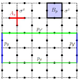
Figure 1: The toric code on a square lattice: The star operator $A_{s}$, shown in red, is the product of $\sigma^{x}$ components of the spins on the four sites connected to the bonds forming a + (star) centered on site $s$. The plaquette operator $B_{p}$, shown in blue, takes the products of $\sigma^{z}$ components of the spins on the four sites at the edges of a plaquette (labeled by $p$). The operators $p_{x}$ and $p_{x^{\prime}}$ are defined as the product of spins $\sigma^{z}$ along the green lines. With PBCs, the Wilson loop order parameter $\gamma(L)$ is $\langle p_{x}\,p_{x^{\prime}}\rangle$, where, in our work here, the distance beween the two green lines should be the largest possible in the system. For a 2D square lattice of even size, this distance is $L/2$, while for a 3D simple cubic lattice it is $\sqrt{2}L/2$. With OBCs, we have to include also the products of boundary spins (along the blue lines), defined as $p_{y}$ and $p_{y^{\prime}}$, and the order parameter $\gamma(L)$ becomes $\langle p_{x}\,p_{x^{\prime}}\,p_{y}\,p_{y^{\prime}}\rangle$.

$A_{s}$ stands for the star operators, namely the product of $\sigma^{x}$ components of the spins around the bonds forming a + (star) at site $s$, and $B_{p}$ denotes the plaquette operators, namely the product of $\sigma^{z}$ components of the spins around the edges of plaquette $p$. These interactions are illustrated in Fig. 1, where an example of the star operator $A_{s}$ is marked as red and the plaquette operator $B_{p}$ is colored with blue. In 3D, the system is defined on a cubic lattice, with similar four-spin plaquette operators but the star operators are upgraded to the product of the six spins on the bonds stemming from a given site.

All star and plaquette operators commute with one another (and therefore with the Hamiltonian), and the ground states of the system have $A_{s}=+1$ and $B_{p}=+1$. Excitations above the ground state take the form of negative stars/plaquettes, with energy penalty $2J_{A}$ and $2J_{B}$ respectively. These defects are referred to as ‘electric’ and ‘magnetic’, and behave like quasiparticles that can only be created and annihilated in pairs, under periodic boundary conditions. They are static under the application of the Hamiltonian, but can otherwise move freely without energy cost through the action of $\sigma^{z}$ or $\sigma^{x}$ operators (for a review, see for instance Ref. savary17, ). In presence of open boundaries, one can easily see that single defects can nucleate or evaporate at the surface.

In this paper we shall focus on the following classical limits of the toric code:

• In 2D, if one takes either $J_{A}\to 0$ or $J_{B}\to 0$, one obtains the classical $\mathbb{Z}_{2}$ lattice gauge model wegner71 ; john79 . This model has no finite temperature transition, and only orders at $T=0$.

• In 3D, the limit $J_{A}\to 0$ yields the classical $\mathbb{Z}_{2}$ gauge model wegner71 ; john79 . This model has a finite temperature phase transition.

• In 3D, the limit $J_{B}\to 0$ yields the version of the $\mathbb{Z}_{2}$ gauge model that we here refer to as the 3D star model claudio08 . This model has no finite temperature transition but orders topologically at $T=0$.

The ordered phases in these models are topological in nature, as reflected, for instance, by a non-zero topological entanglement entropy claudio07 ; claudio08 . Here we will characterize the dynamic topological ordering using the Wilson loops, illustrated in Fig. 1 for 2D systems. For the 3D star model we will use a higher-dimensional generalization of the Wilson loop.

III 3D $\mathbb{Z}_{2}$ gauge model at $T=T_{c}$

The 3D $\mathbb{Z}_{2}$ lattice gauge model exhibits a topological phase transition at $T_{c}/J_{B}=1.313346$ john79 ; wegner71 ; claudio08 (where we set $J_{B}=1$ hereafter). The transition is in the same universality class as the standard 3D Ising model, and yet it has no local order parameter in the original spin degrees of freedom. The mapping between the two models is a duality between low- and high-temperature partition functions; therefore the thermodynamic behavior of the two models is the same, but there is no obvious relation between their stochastic (Monte Carlo) dynamics. The order parameter for the 3D $\mathbb{Z}_{2}$ lattice gauge theory is a product of spins across the entire system, namely a system-spanning Wilson loop. For $T<T_{c}$, the order parameter decays exponentially with the perimeter of the contour, $\langle W\rangle\sim e^{-\alpha L}$, known as the ‘perimeter law’, in contrast to the ‘area law’ for $T>T_{c}$, where the order parameter decays exponentially with the area of the contour, $\langle W\rangle\sim e^{-\beta L^{2}}$. john79

In our simulations, we define a specific Wilson loop as our order parameter:

$$\gamma(L)=\langle p_{x}\,p_{x^{\prime}}\rangle\,,\qquad p_{x}=\prod_{i\in{\cal L}_{x}}\sigma_{i}^{z}\,,$$ (4)

where $p_{x}$ and $p_{x^{\prime}}$ are the products of $\sigma^{z}$ spins along two lattice lines ${\cal L}_{x}$ and ${\cal L}_{x^{\prime}}$ which are farthest away from each other within the system, as demonstrated in Fig. 1 for a 2D system. In 3D, the largest possible distance is $\sqrt{2}L/2$. Exploiting translation invariance, $\gamma(L)$ is averaged over $x$ and $x^{\prime}$ respecting the maximum distance condition.

III.1 Simulated annealing

Here and in the rest of the work we use SA simulations. We first prepare the system in equilibrium at a relatively high initial temperature $T_{\rm ini}$ (where a small number of Monte Carlo sweeps is enough to reach equilibrium when starting from a random configuration), and then we decrease the temperature to the final value $T_{f}$ via the protocol

$$T(t)=T_{f}+(T_{\rm ini}-T_{\rm f})\,\left(1-t/t_{\rm q}\right)^{r}\,,$$ (5)

where $r=1$ stands for the standard SA where temperature decreases linearly. In general, one can vary the value of $r$ in order to disentangle the exponents ($z$ and $\nu$) shown in the KZ scaling. liu14 ; rubin17 In this study, we only consider the standard $r=1$ protocol, since the value of $\nu$ is the same as the one in the 3D Ising model, which is known to high accuracy, $\nu=0.62999(5)$ showk14 . We consider $T_{\rm ini}=1.1T_{c}$ and $T_{f}=T_{c}$. The total number of Monte Carlo steps during the SA process is denoted by $t_{q}$, and one step (the unit of time) corresponds to a total of $N=L^{3}$ Metropolis single spin flip attempts. The annealing rate (or velocity) $v$ is then defined as

$$v=(T_{\rm ini}-T_{\rm f})/t_{\rm q}\,.$$ (6)

We simulate systems with sizes $L=8,10,12,16,24$ and $32$. For each system size, we perform SA runs at various sweeping rates $v$. The range of velocities varies for different system sizes between about $10^{-6}$ and $10^{-2}$. We measure the order parameter $\gamma(L)$ as defined in Eq. (4) at various temperatures during each SA process, averaging over around $10^{4}$ repeats. Note here that each SA process is independent, with different initial configurations as well as distinct random numbers during the MC updates.

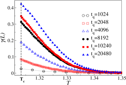
Figure 2: The topological order parameter $\gamma(L)$ for a system with $N=16^{3}$ spins as a function of the temperature, computed at various total times $t_{q}$ for annealing from $T=1.1T_{c}$ to $T_{c}$. The error bars are smaller than the symbol sizes.

Figure 2 shows examples of the order parameter $\gamma(L)$ for system size $L=16$ at various quenching rates. The slower we perform SA, the closer the system gets to its equilibrium state, i.e., the more ordered it becomes. The vertical dashed line indicates the last step taken in our SA runs, ending when $T=T_{c}$. Since the simplest one-parameter KZ scaling function (discussed below) involves only the measurement at $T_{c}$, in the following we only focus on the last data point of the SA process at $T=T_{c}$ for each annealing velocity.

III.2 Dynamic scaling

In the generalized KZ non-equilibrium finite-size scaling form for a physical observable $A$, the dynamic finite-size scaling of $A$ as a function of annealing velocity is,

$$A(L,v)\sim A_{\rm eq}(L)f(v/v_{KZ})\,,$$ (7)

where $A_{\rm eq}(L)$ denotes the equilibrium finite-size value at $T_{c}$. Normally this value is a power law in the linear size of the system $L$. However, we propose that a simple generalization of the KZ form applies straightforwardly to other functions of $L$, as relevant to this work.

For linear SA, the KZ velocity has the form given in Eq. (2), $v_{KZ}\sim L^{-z-1/\nu}$. Considering the ‘perimeter law’ associated with the Wilson loop order parameter $\gamma(L)$ at $T_{c}$, we expect $\gamma(L)$ measured at the critical point to take the form

$$\gamma(L,v)\sim e^{-\alpha L}f(vL^{z+\frac{1}{\nu}})\,,$$ (8)

where $\nu$ is the critical correlation-length exponent and $z$ is the dynamic critical exponent.

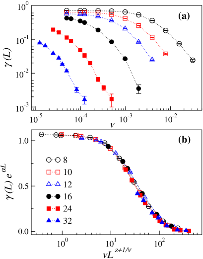
Figure 3: (a) Behavior of the topological order parameter $\gamma(L)$ measured at $T_{c}$, shown on a log-log plot under various quenching rates for system sizes $L=8$, $10$, $12$, $16$, $24$, and $32$ (with the curves decreasing as $L$ increases, as expected for perimeter law behavior). (b) Scaling collapse of $\gamma(L)$ as a function of velocity, based on Eq. (8) and shown on a semi-log plot. The optimal value of $z$ for the data collapse is $z\approx 2.70(3)$.

Figure 3(a) shows the behavior of $\gamma(L)$ for various annealing rates and system sizes from $L=8$ to $L=32$. Figure 3(b) shows the velocity scaling of $\gamma(L)$ based on the KZ scaling function. We vary the values of exponents $z+1/\nu$ and $\alpha$ to collapse the data according to Eq. (8). The best fit yields the optimal values $z+1/\nu=4.29(3)$, $\alpha=0.052(1)$. As $\nu\approx 0.63$, we obtain $z=2.70(3)$. The statistcal errors were determined by a bootstrap analysis. For further details on the data-collapse procedures we refer to Refs. liu14, and rubin17, .

Previous Monte Carlo studies of the equilibrium relaxation (autocorrelation) time at $T_{c}$ gave $z=2.5(2)$ ben-av90 . Thus, our result for $z$ agrees with the previous value within error bars, but we improve the statistical precision by one digit. The general expectation is that the dynamic exponent appearing within the out-of-equilibrium KZ framework should indeed be the same as the one at equilibrium when $T_{c}>0$ (while for systems with $T_{c}=0$ this is not the case rubin17 ; xu17 ). The good collapse of the data reveals that, as with other continuous phase transitions described by local order parameters biroli10 ; chandran12 ; liu14 ; liu15 , KZ scaling also works for topological phase transitions devoid of a local order parameter. We stress again that the standard KZ scaling form in this case is also modified by the exponential form of the equilibrium size-dependence in Eq. (8).

Recall that the mapping between the 3D $\mathbb{Z}_{2}$ lattice gauge model and the 3D Ising model is a duality between the partition functions, and thus has no dynamical implications. Moreover, the dynamic exponent is not an intrinsic property of a model, as it also depends on the specific update algorithm. While they share the same thermodynamic critical properties, it is not surprising that they have different dynamical exponents, $z\approx 2.7$ and $z\approx 2.0$ wansleben87 ; wang95 , for the gauge model and standard 3D Ising model, respectively. There may exist an update algorithm for the 3D $\mathbb{Z}_{2}$ lattice gauge model that matches exactly with the local update of the 3D Ising model. However, as the duality mapping between the two models is highly nontrivial, we expect the algorithm to be highly nontrivial as well.

Note also that the out-of-equilibrium SA approach with KZ scaling circumvents the need to ensure that the system is in equilibrium when using autocorrelation functions to estimate the equilibrium dynamic exponent. Each repetition of the SA procedure represents a statistically independent contribution to the estimated mean values. Thus, the only potential source of systematic errors is corrections to scaling in the analysis. Based on the good data collapse for large systems at the known value of $T_{c}$, we judge that the impact of scaling corrections should be small in the above results for the 3D $\mathbb{Z}_{2}$ lattice gauge model.

IV $T=0$ topological order with periodic boundary conditions

In this section we study models that have no finite-temperature phase transition and topological order only forms at $T=0$, when the defect density vanishes identically at equilibrium. Namely, we consider the 3D star model claudio08 and the 2D $\mathbb{Z}_{2}$ lattice gauge model. In addition, we also consider their natural reduction down to 1D; the standard ferromagnetic Ising chain.

IV.1 Failure of the Kibble-Zurek mechanism

For systems that order only at $T=0$, we cannot apply directly the standard KZ scaling forms, because when $T\rightarrow 0$ the correlation length diverges exponentially, $\xi\sim\exp(c/T)$, instead of following the power-law behavior expected at finite-$T$ continuous phase transitions. In principle the exponential form is not an issue in itself, as apparent in the detailed derivation of the KZ scaling forms in Ref. liu14, (see also Ref. chandran12, ). As long as there is a known relationship between the correlation length and the relaxation time, a criterion for quasi-static equilibrium—giving a critical velocity separating slow and fast processes, equivalent to Eq. (2)—can be obtained. For example, in the 1D Ising model the correlation length has exactly the form $\xi\sim\exp(c/T)$. If one assumes that the relaxation time is a power of this length, $\tau\sim\xi^{z}$, as expected with $z=2$ based on the fact that the domain walls perform 1D random walks, one finds that the critical KZ velocity is $v_{\rm crit}\sim L^{-z}\ln^{-2}(L)$.

However, this result is incorrect, differing by a factor of $\ln(L)$ from the known rigorous expression obtained by Krapivsky for this model paul10 . The reason for the failure of this simplistic approach is that the correlation length is not changing smoothly in a given realization of the annealing process in a finite system at the last stages of equilibration. When the number of domain walls (defects) is small, the (kink-antikink) annihilation of a defect pair leads to large jumps in the correlation length. For instance, the very last annihilation process in a 1D Ising model of finite size $L$ produces a jump in the correlation length from $\xi=L/2$ to $\xi=L$. On the contrary, a continuous (in the large $L$ limit) growth of the correlation length all the way to $\xi=L$ is a key assumption in the derivation of the KZ scaling expressions liu14 .

IV.2 Scaling theory for defect annihilation

We are nonetheless able to obtain a finite-size scaling form for the order parameter in these systems, as they are ramped down to zero temperature, by looking more closely at the nature of their defects and how order emerges as the defect density vanishes. As in the 1D Ising model, the excitations at low $T$ in the 2D $\mathbb{Z}_{2}$ gauge model and the 3D star model also take the form of stochastically itinerant non-interacting point-like quasiparticles. The point-like nature of the excitations is closely related to the absence of a phase transition. Indeed, the energy-free (diffusive) motion of these quasiparticles is able to change the value of the (topological) order parameter. Therefore, whenever excitations are present in the system, the order parameter remains vanishingly small. This is clearly the case at all $T>0$ in the thermodynamic limit. A non-vanishing order parameter can, however, appear as a finite-size effect when the temperature becomes so low that on average less than one pair of defects is left in the system. This behavior is controlled by the very final stage of relaxation into the topologically ordered state, namely the disappearance of the last excitations. With periodic boundary conditions, this corresponds to the process where the last pair of defects meet and annihilate.

Considering SA with linear sweeps down to $T_{f}=0$, to quantify the longest time scale we can assume that the system remains in equilibrium (with vanishingly small order parameter) down to a threshold temperature $T_{\rm th}$ where the number of defects left in the (finite) system is of order $1$,

$$\exp\left(-\frac{\Delta}{T_{\rm th}}\right)\sim L^{-d}.$$ (9)

Here $\Delta$ is the bare cost of a defect (e.g., the cost of a single domain wall in the 1D Ising model), and $d=1,2,3$ is the dimensionality of the system. Only if the sweep continues for a sufficiently long time from $T_{\rm th}$ down to $T=0$ is the order parameter finally able to acquire a finite expectation value via the annihilation of the last two remaining defects. Therefore, the scaling behavior of the order parameter at the end of the sweep ($T=0$) is controlled by this regime.

Taking $T_{\rm f}=0$ and $r=1$ in Eq. (5), the time dependence of the temperature in a SA sweep in $t\in(0,t_{\rm q})$ takes the form

$$T(t)=T_{\rm ini}\left(1-\frac{t}{t_{\rm q}}\right),$$ (10)

where $T_{\rm ini}$ is the initial temperature and $t_{q}$ is the number of total quench steps. The sweep velocity is thus $v=T_{\rm ini}/t_{\rm q}$ and the time it takes from $T_{\rm th}$ to $T=0$ is

$$\Delta t=t_{q}-t_{\rm th}=\frac{T_{\rm th}}{v}\,.$$ (11)

Inserting the expression for $T_{\rm th}$ from Eq. (9) into the above expression, we get

$$\Delta t\sim\frac{\Delta}{v\ln(L)}\,,$$ (12)

which we can now relate to the time scale of defect annihilation. The system develops a non-vanishing order parameter in the span of time $\Delta t$ only if the last quasiparticles in the system meet and annihilate.

As the quasiparticles are non-interacting, their motion is diffusive and the time scale for annihilation $\tau_{\rm annihilation}$ should depend on dimensionality and system size condamin05 :

$$\tau_{\rm annihilation}\sim\begin{cases}L^{2},~{}~{}~{}&d=1\\ L^{2}\ln(L),~{}~{}~{}&d=2\\ L^{3},~{}~{}~{}&d=3\,.\end{cases}$$ (13)

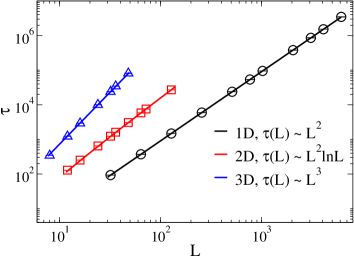
Figure 4: Behavior of the mean time $\tau$ required for annihilation of the last pair of defects through random walks vs the system size $L$ in 1D (black), 2D (red) and 3D (blue) lattices with PBCs. The solid curves are fits based on the expected scaling forms in Eq. (13).

We numerically tested these scaling laws by considering the case of two defects (with random initial conditions) performing random walks on 1D, 2D and 3D lattices with PBCs. We measured the average relaxation time $\tau$, which is the number of total steps the defects take before they meet and annihilate (one step corresponding to one lattice move of each defect). Our results are presented in Fig. 4. The excellent agreement with the scaling form in Eq. (13) demonstrates the lack of significant finite-size corrections even for the smallest system sizes considered in this work—an important benchmark for the interpretation of our results on topological systems below.

The probability that the system develops a non-vanishing order parameter in an SA run is controlled by the ratio $\Delta t/\tau_{\rm annihilation}$. Combining Eqs. (12) and (13), this ratio can be expressed in a KZ-like scaling form as

$$\frac{\tau_{\rm annihilation}}{\Delta t}=\frac{v}{v_{\rm crit}}\;,$$ (14)

where

$$v_{\rm crit}\sim\begin{cases}L^{-2}\ln^{-1}(L),~{}~{}~{}&d=1,\\ L^{-2}\ln^{-2}(L),~{}~{}~{}&d=2,\\ L^{-3}\ln^{-1}(L),~{}~{}~{}&d=3\,.\end{cases}$$ (15)

We thus expect that the dynamic finite-size scaling function of an appropriate order parameter $M$ in each of the systems considered here takes the form

$$M\sim f(v/v_{\rm crit})\,,$$ (16)

which is formally similar to the KZ scaling ansatz but with critical velocities that cannot be derived within that formalism.

We note that the case of the 1D Ising chain was previously studied analytically in a somewhat different way in Ref. paul10, , and the domain wall density there indeed shows a scaling form consistent with our Eqs. (15) and (16). Another study related to our work is Ref. freeman14, , where the finite-size scaling of the 2D toric code was considered using an effective classical model in contact with a thermal reservoir. There the focus was on the time scale on which topological order is destroyed at fixed temperature through topological point defects undergoing nontrivial random walks; this is different from the case studied here where we consider the opposite process of topological ordering under SA down to $T=0$. The time scales in our work and in Ref. freeman14, are therefore not the same.

IV.3 Simulated annealing results

We performed SA runs (setting $T_{\rm ini}=2$) with various annealing velocities for the 1D Ising model, the 2D $\mathbb{Z}_{2}$ lattice gauge model and the 3D star model, using several system lengths $L$ in each case. For the Ising chain, we choose the commonly-used squared magnetization, $m^{2}$, as our order parameter,

$$m^{2}=\left\langle\frac{1}{L}\sum_{i=1}^{L}\sigma_{i}\right\rangle^{2}\,.$$ (17)

For the 2D $\mathbb{Z}_{2}$ gauge model, we use a Wilson loop order parameter similar to that introduced for the 3D case in Sec. III and illustrated in Fig. 1. The only difference from the 3D case is that now the farthest distance between the lines ${\cal L}_{x}$ and ${\cal L}_{x^{\prime}}$ is $L/2$ instead of $\sqrt{2}L/2$.

For the 3D star model, the topological state has a different nature with respect to a $\mathbb{Z}_{2}$ gauge model, and the role of Wilson loops is played by products of spins around (dual) closed surfaces that are locally perpendicular to and bisect the bonds of the original lattice. The simplest such surface is a unit dual cube surrounding a single vertex on the original lattice, and the six spins on the bonds stemming from that vertex live respectively at the centers of the six faces of the cube. In the ground state, the product of the six spins is $1$ (namely, the product of the six spins on the faces of the dual cubic surface). For a detailed discussion of these topological structures we refer the reader to Ref. claudio08, . Here we follow that reference and introduce the corresponding order parameter as the product of all the spins on two parallel (dual) lattice planes, ${\cal P}_{x}$ and ${\cal P}_{x^{\prime}}$, at, say, fixed $x$ and $x^{\prime}$ values on the lattice (see Fig. 5).

Figure 5: Illustration of the topological order parameter of the 3D star model with periodic and open boundary conditions. For PBCs the order parameter $\pi(L)$ is the average of surface-surface correlations, indicated in blue. For OBCs the order parameter should include also the product of spins on the boundaries between these two surfaces, shown in orange, so as to form a closed surface.

For a system with periodic boundary conditions, the product of the spins on the two planes equals the product of all dual unit cubes around the vertices in between the two planes. Therefore, in the ground state the product takes value $1$. This product acts as a topological order parameter, similar to the Wilson loop used for the Ising gauge models with plaquette interactions.

For convenience, we denote as $s_{x}$ and $s_{x^{\prime}}$ the products of all the spins on each of the two planes ${\cal P}_{x}$ and ${\cal P}_{x^{\prime}}$, separately, and we define

$$\pi(L)=\langle s_{x}\,s_{x^{\prime}}\rangle\,,\qquad s_{x}=\prod_{i\in{\cal P}_{x}}\sigma_{i}^{z}\,,$$ (18)

as a closed-surface analog of the Wilson loop. Here the distance between the two surfaces ${\cal P}_{x}$ and ${\cal P}_{x^{\prime}}$ is taken to be maximal, namely $L/2$.

The behavior of the three order parameters after rescaling according to Eqs. (15) and (16) is presented in Fig. 6.

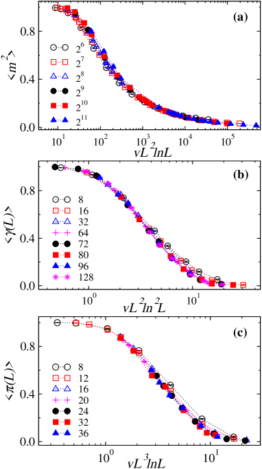
Figure 6: Scaling behavior on semi-log plots of the order parameters in (a) the 1D Ising chain, (b) the 2D $\mathbb{Z}_{2}$ gauge model, and (c) the 3D star model with PBCs.

We find good scaling collapse of the data, and the trend is a clear improvement with increasing system size, suggesting that the scaling functions we propose are indeed correct. In principle, a scale factor $L_{0}$ inside the logarithms of the scaling arguments could also be included, $\ln(L/L_{0})$, but we find that the optimum value of this factor is close to $1$ and the data collapse is not significantly improved. We therefore did not include such a scale factor in the figure and further below.

One can notice that the data collapse gets worse when $v\gg v_{\rm crit}$, which is expected as the scaling form was derived under the assumption that the system remains at equilibrium down to $T_{\rm th}$. This assumption breaks down at high velocity, in such a way that the scaled data peel off from the common scaling form at a point that moves to the right as the system size increases. This is similar to what happens in KZ scaling, as discussed in Ref. liu14, . We conclude that the low-$T$ dynamics of these systems is indeed controlled by defect-defect annihilation processes of free random walking quasiparticles.

V $T=0$ topological order with open boundary conditions

In this section, we discuss how OBCs affect the dynamics of the topological order parameters for the systems studied in Sec. IV. With PBCs, the only way for defects to vanish is through defect pair annihilation. With OBCs, however, defects can diffuse to and disappear through the open boundaries—thus single defects can “evaporate”.

V.1 Scaling of boundary evaporation

Whereas the time for pair annihilation scales as $L^{2}$, $L^{2}\ln L$, and $L^{3}$ in $d=1$, $2$, and $3$ [see Eq. (13)], defects can reach the boundary within a typical time scale

$$\tau_{\rm boundary}\sim L^{2}\,,$$ (19)

irrespective of dimensionality sidbook . Clearly, when comparing the two kinds of dynamics, boundary evaporation takes either equal (1D) or shorter (2D and 3D) time. Therefore, the low-temperature dynamics should be dominated by boundary processes, leading to a different critical velocity in the dynamic scaling function $f(v/v_{\rm crit})$. Following the discussion in the previous section, upon replacing $\tau_{\rm annihilation}$ by $\tau_{\rm boundary}$, we obtain a form for $v_{\rm crit}$ that is universal for 1D, 2D and 3D lattices with OBCs:

$$v_{\rm crit}\sim L^{-2}\ln^{-1}(L)\,.$$ (20)

Notice that the order parameters for the 2D $\mathbb{Z}_{2}$ lattice gauge model $\gamma(L)$ and the 3D star model $\pi(L)$ have to be redefined after switching to OBCs (while for the 1D Ising chain it remains the same). For the 2D $\mathbb{Z}_{2}$ gauge model, as illustrated in Fig. 1, in addition to the two line operators $p_{x}$ and $p_{x^{\prime}}$, we also need to include the spins on the boundaries between the two lines, i.e., $p_{y}$ and $p_{y^{\prime}}$, in order to form a closed loop. Therefore, the order parameter becomes,

$$\gamma(L)=\langle p_{x}\,p_{x^{\prime}}\,p_{y}\,p_{y^{\prime}}\rangle\,.$$ (21)

For the 3D star model, as illustrated in Fig. 5, in addition to the two surface operators $s_{x}$ and $s_{x^{\prime}}$, we need to include the product of spins on the boundary surfaces in between, to form a closed surface.

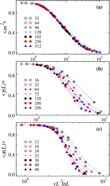
Figure 7: Scaling of the order parameters for OBC systems for (a) the 1D Ising model, (b) the 2D $\mathbb{Z}_{2}$ gauge model, and (c) the 3D star model. In all cases we have used the universal scaling form $f(v\,L^{2}\ln L)$.

Figure 7 shows the scaling behavior of the order parameters with OBCs. The data are plotted according to the new universal scaling form $f(v/v_{\rm crit})$, where $v/v_{\rm crit}\sim v\,L^{2}\ln L$, due to the (faster) dynamical process whereby defects reach the open boundaries by random walking and evaporate. The excellent collapse in panel (a) is expected due to the fact that the two relaxation processses lead to the same scaling form in 1D. The scaling collapse in panels (b) and (c), 2D and 3D respectively, is far less satisfactory. The data points for small system sizes show a substantial deviation from the predicted behavior. As system size increases, the data collapse gradually improves, suggesting that the scaling form is correct in the thermodynamic limit but finite-size effects are far stronger with OBCs than PBCs. This is likely due to the contributions from the two dynamical processes with time scales that diverge from one another for $L\gg 1$, but are in fact quite close for small systems (indeed $\tau_{\rm annihilation}/\tau_{\rm boundary}=\ln(L)$ in 2D, which is just $\simeq 4.6$ for $L=100$; and $\tau_{\rm annihilation}/\tau_{\rm boundary}=L$ in 3D, where we can only access relatively small system sizes overall).

V.2 Combining evaporation and annihilation

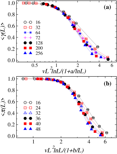
Figure 8: Modified velocity scaling of the order parameter for the 2D and 3D OBC systems, combining effectively both relaxation processes (pair annihilation and boundary/surface evaporation). (a) Results for the 2D $\mathbb{Z}_{2}$ lattice gauge model, with the velocity scaled as $v\,L^{2}\ln(L)(1+a/\ln(L))^{-1}$ with $a$=2.4(2), and (b) for the 3D star model with rescaling $\sim v\,L^{2}\ln(L)(1+b/L)^{-1}$ with $b=2.2(3)$. In (a) the smallest system was excluded from the data-collapse analysis, while in (b) all sizes were used.

In order to account for the two different defect removal processes, we consider a modified scaling approach for the 2D and 3D systems. The rate of defect depletion is the sum of those for the two separate channels (defect annihilation and evaporation at the boundary), yielding the effective rate

$$\tau^{-1}_{\rm eff}=\tau^{-1}_{\rm boundary}+\tau^{-1}_{\rm annihilation}\;.$$ (22)

From this total rate, we obtain the effective critical velocity scale, which is the sum of the critical velocities for the two separate processes.

Recall that, for the 2D case, the critical velocities for the process of defect annihilation and boundary evaporation are given by $v_{\rm crit,a}\sim L^{-2}\ln^{-2}(L)$ and $v_{\rm crit,e}\sim L^{-2}\ln^{-1}(L)$, respectively. We therefore propose a combined critical velocity of the form

$$v_{\rm crit} \sim L^{-2}\ln^{-1}(L)+aL^{-2}\ln^{-2}(L)$$

$$\sim L^{-2}\ln^{-1}(L)\left(1+\frac{a}{\ln(L)}\right),$$ (23)

where $a$ is a fitting parameter that accounts for ${\cal O}(1)$ prefactors in the $L$ dependence of the velocities. The modified argument of the scaling function in 2D should then take the form

$$(v/v_{\rm crit})_{\rm 2D}\sim v\,L^{2}\ln(L)\left(1+\frac{a}{\ln(L)}\right)^{-1}.$$ (24)

Given that the two processes contribute additively to the overall rate in Eq. (22) we expect $a>0$.

Analogously, for the 3D star model, the improved scaling argument should take the form

$$(v/v_{\rm crit})_{\rm 3D}\sim v\,L^{2}\ln(L)\left(1+\frac{b}{L}\right)^{-1},$$ (25)

where $b$ again is a fitting parameter that is expected to be positive. Fig. 8 shows the analysis for both cases based on the new scaling functions, which indeed improve the data collapse considerably (especially in the 2D case). The best data collapse yields $a=2.4(2)$ and $b=2.2(3)$, both positive as expected.

VI Discussion

In this paper we studied the dynamical scaling behavior of several classical topological systems using SA with varying sweeping rates. For the 3D $\mathbb{Z}_{2}$ lattice gauge model, which undergoes a topological phase transition at finite temperature, the dynamical scaling of its order parameter can be understood as a simple generalization of the KZ mechanism to an order parameter with exponential size dependence at $T_{c}$ (instead of the power law applying at standard continuous phase transitions). To our knowledge, this is the first time that KZ theory has been applied and tested numerically on a classical system with a continuous topological phase transition devoid of a local order parameter. Our result for the dynamical exponent of the system, $z=2.70(3)$, is consistent within error bars (which are an order of magnitude smaller in our work) with a previously published value based on equilibrium autocorrelations ben-av90 , thus supporting the notion of a common exponent describing the equilibrium and the out-of-equilibrium relaxation.

In contrast to systems with continuous phase transitions with $T_{c}>0$, we point out that finite-size scaling functions based on the generalized KZ ansatz do not apply to transitions into topological phases that only exist at zero temperature. In these systems the correlation length diverges exponentially in temperature as $T\to 0$, and at the last stage of ordering the finite-size correlation length jumps when topological defects (the end-points of strings) finally disappear. We studied examples of such systems, namely, the 2D $\mathbb{Z}_{2}$ lattice gauge model and the 3D star model. For completeness we also studied a simpler but analogous system in 1D: the standard Ising chain that was also previously investigated by Krapivsky paul10 . The stochastic dynamics of ordering in these systems is dominated by the diffusion of the end-points of open strings, and we proposed scaling functions that are obtained from dynamical modeling of the annihilation processes of these topological point defects through random walks. We find excellent agreement between the proposed scaling laws and numerical SA simulations, suggesting that we have correctly identified and modelled the relevant relaxation processes in these systems. Note also that while the numerical analysis cannot strictly distinguish between the KZ and the defect-annihilation forms, because they differ only logarithmically, our physical arguments against the standard KZ scaling mechanism are unambiguous.

We also studied the effect of open boundaries, where individual defects can evaporate. We find that defect evaporation dominates over pair annihilation for large enough systems. For system sizes that are numerically accessible, a scaling approach combining the different time-scales of the two processes is needed to fit the data.

It is important to contrast our results for the $T=0$-ordering models with the KZ scenario. A naive application of the KZ mechanism according to the derivation in Appendix A of Ref. liu14, gives $v_{\rm crit}\sim L^{-2}\ln^{-2}(L)$ if we assume forms of the correlation length and relaxation time scale appropriate for the $T_{c}=0$ systems considered here: $\xi\sim\exp(c/T)$ and $\tau\sim\xi^{z}$ with $z=2$. Interestingly, comparing with the forms we have obtained based on the defect annihilation scenario, Eq. (15), the results are exactly the same in 2D, while they differ by a factor $\ln(L)$ and $L\ln(L)$ in 1D and 3D, respectively. For OBCs, the above KZ result (which is insensitive to boundary conditions) differs by $\ln(L)$ from the correct form in all dimensions.

Our results demonstrate that a scaling collapse in the ordering behavior of a many body system is not per se evidence of KZ scaling. On the contrary, scaling can arise from the dynamical behavior of the excitations as the system relaxes into its ordered state. By an appropriate effective modeling of these excitations, it is possible to infer the dynamical scaling form of the order parameter. A tell tale sign of the difference between KZ-driven and defect-driven scaling may be observable when we compare the behavior of open and closed boundary conditions, as we illustrate using examples in $d=1,2,3$.

Finally, our work also provides analytical estimates (and corresponding numerical verification) of the time scales relevant for the onset of topological order as $T\to 0$ (following linear ramps in temperature). We remark that these time scales are indeed the ones required to prepare the toric code in 2D and 3D in a topologically ordered ground state devoid of any excitations. Even though the toric code is but a toy model for topological quantum computing, modeling of excitations in a manner similar to the one presented in our work may be relevant to preparing quantum topological states in a potential experimental setting for quantum information processing.

References

- (1) X.-G. Wen, Int. J. Mod. Phys. B 4, 239 (1990); Adv. Phys. 44, 405(1995) ; Phys. Rev. B 65, 165113 (2002).
- (2) F. D. M. Haldane and E. H. Rezayi, Phys. Rev. B 31, 2529 (1985).
- (3) X.-G. Wen and Q. Niu, Phys. Rev. B 41, 9377 (1990).
- (4) E. Dennis, A. Kitaev, A. Landahl, and John Preskill, J. Math. Phys. 43, 4452 (2002).
- (5) C. Nayak, S. H. Simon, A. Stern, M. Freedman and S. Das Sarma Rev. Mod. Phys. 80 1083 (2008).
- (6) A. Kitaev, Ann. Phys. 321, 2 (2006). Ann. Phys. N.Y. 303, 2 2003
- (7) F. J. Wegner, J. Math. Phys. 12, 2259 (1971).
- (8) J. B. Kogut Rev. Mod. Phys. 51.659 (1979).
- (9) S. Wansleben, J. Phys. A. Gen. 18, L211 (1985).
- (10) C. Castelnovo and C. Chamon, Phys. Rev. B 76, 174416 (2007).
- (11) A. J. Macdonald, P. C. W. Holdsworth, and R. G. Melko, J. Phys.: Condens. Matter 23 164208 (2011).
- (12) C. D. Freeman, C. M. Herdman, D. J. Gorman, K. B. Whaley, Phys. Rev. B 90, 134302 (2014).
- (13) T. W. B. Kibble, J. Phys. A: Math. Gen. 9, 1387 (1976).
- (14) W. H. Zurek, Nature (London) 317, 505 (1985).
- (15) W. H. Zurek, Phys. Rep. 276, 177 (1996).
- (16) A. Polkovnikov, Phys. Rev. B 72, 161201(R) (2005).
- (17) C. De Grandi, V. Gritsev, and A. Polkovnikov, Phys. Rev. B 81, 012303 (2010).
- (18) G. Biroli, L. F. Cugliandolo, and A. Sicilia, Phys. Rev. E 81, 050101(R) (2010).
- (19) A. Jelic and L. F. Cugliandolo, J. Stat. Mech. 2011, P02032 (2011).
- (20) J. Hamp, A. Chandran, R. Moessner, and C. Castelnovo, Phys. Rev. B 92, 075142 (2015).
- (21) A. Polkovnikov, K. Sengupta, A. Silva, and M. Vengalattor, Rev. Mod. Phys. 83 863 (2011).
- (22) H. Ricateau, L. F. Cugliandolo, and M. Picco, J. Stat. Mech. (2018) 013201.
- (23) C. De Grandi, A. Polkovnikov, and A. W. Sandvik, Phys. Rev. B 84, 224303 (2011).
- (24) A. Chandran, A. Erez, S. S. Gubser, and S. L. Sondhi, Phys. Rev. B 86, 064304 (2012).
- (25) F. Zhong and Z. Xu, Phys. Rev. B 71, 132402 (2005).
- (26) C.-W. Liu, A. Polkovnikov, and A. W. Sandvik, Phys. Rev. B 89, 054307 (2014).
- (27) G. Lamporesi, S. Donadello, S. Serafini, F. Dalfovo, and G. Ferrari, Nature Phys. 9, 656 (2013).
- (28) L. W. Clark, L. Feng, C. Chin, Science 354, 606 (2016).
- (29) C.-W. Liu, A. Polkovnikov, A. W. Sandvik, and A. P. Young, Phys. Rev. E 92, 022128 (2015).
- (30) C.-W. Liu, A. Polkovnikov, and A. W. Sandvik, Phys. Rev. Lett. 114, 147203 (2015).
- (31) S. J. Rubin, N. Xu, and A. W. Sandvik, Phys. Rev. E 95, 052133 (2017).
- (32) N. Xu, K.-H. Wu, S. J. Rubin, Y.-J. Kao, A. W. Sandvik, Phys. Rev. E 96, 052102 (2017).
- (33) R. Ben-Av, D. Kandel, E. Katznelson, P.G. Lauwer, and S. Solomon, J. Stat. Phys, Vol. 58, 125 (1990).
- (34) L. Savary and L. Balents, Rep. Prog. Phys. 80, 016502 (2017).
- (35) C. Castelnovo and C. Chamon, Phys. Rev. B 78,155120 (2008).
- (36) S. El-Show, M. F. Paulos, D. Poland, S. Rychkov, D. Simmons-Duffin, and A. Vichi, J. Stat. Phys. 157, 869 (2014).
- (37) S. Wansleben and D. P. Landau, Journal of Applied Physics 61, 3968 (1987).
- (38) F. Wang, N. Hatano, and M. Suzuki, J. Phys. A: Math. Gen. 28, 4543 (1995).
- (39) S. Condamin, O. Benichou, and M. Moreau, Phys. Rev. Lett. 95, 260601 (2005).
- (40) P. L. Krapivsky, J. Stat. Mech. 2010, P2014 (2010).
- (41) S. Redner, A Guide to First-Passage Processes, Cambridge University Press (Cambridge, 2001).