Stellar Wakes from Dark Matter Subhalos

Abstract

We propose a novel method utilizing stellar kinematic data to detect low-mass substructure in the Milky Way’s dark matter halo. By probing characteristic wakes that a passing dark matter subhalo leaves in the phase space distribution of ambient halo stars, we estimate sensitivities down to subhalo masses $\sim 10^{7}\,M_{\odot}$ or below. The detection of such subhalos would have implications for dark-matter and cosmological models that predict modifications to the halo-mass function at low halo masses. We develop an analytic formalism for describing the perturbed stellar phase-space distributions, and we demonstrate through simulations the ability to detect subhalos using the phase-space model and a likelihood framework. Our method complements existing methods for low-mass subhalo searches, such as searches for gaps in stellar streams, in that we can localize the positions and velocities of the subhalos today.

Introduction.—The Standard Cosmological Model ($\Lambda$CDM), based on cold dark matter (CDM) and a cosmological constant ($\Lambda$), predicts that the otherwise homogeneous primordial plasma features small density perturbations with a nearly scale invariant spectrum. After dark matter (DM) begins to dominate the energy density of the Universe, these perturbations begin to collapse, forming a hierarchical spectrum of DM structures today. This spectrum is predicted to extend to subhalo masses well below those of dwarf Galaxies, $M_{\text{sh}}\sim 10^{9}\,M_{\odot}$, which are the least-massive DM subhalos observed so far. Discovering DM subhalos with even lower mass is complicated by the fact that such objects are not expected to host many stars. Finding such subhalos is of the utmost importance for a number of reasons: (i) their existence is a so-far untested prediction of $\Lambda$CDM Springel:2008cc , (ii) certain particle and cosmological models for DM, including warm DM Colin:2000dn ; Bode:2000gq ; Viel:2005qj , fuzzy DM Hu:2000ke ; Li:2013nal ; Hui:2016ltb , and self-interacting DM Spergel:1999mh ; Wandelt:2000ad ; Kaplinghat:2013kqa , predict drastic deviations from the $\Lambda$CDM prediction for the halo-mass function, which describes the number of halos as a function of mass, at scales below the dwarf scale, and (iii) low-mass and nearby subhalos could provide invaluable targets for indirect searches for DM annihilation and decay.

In this work, we propose a novel method for finding low-mass DM subhalos. DM subhalos perturb the phase-space distribution of stars as they propagate through the local Galaxy. These perturbations, which we dub “stellar wakes”, are a key signature of low-mass subhalos that may be observable with upcoming data from e.g. the Gaia mission 2001A&A…369..339P , the Large Synoptic Survey Telescope (LSST) 2009arXiv0912.0201L , and the Dark Energy Survey (DES) 2005astro.ph.10346T , combined with existing surveys from, for example, the Sloan Digital Sky Survey (SDSS) Juric:2005zr . In the left panel of Fig. 1, we show an example of the perturbed stellar phase-space distribution caused by a $\sim 2\times 10^{7}\,M_{\odot}$ subhalo. Stars are pulled towards the subhalo as it passes, leaving behind distinct features in their velocity distribution and, to a lesser extent, in their number density distribution.

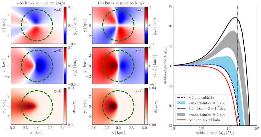
Figure 1: (Left) Moments of the stellar phase-space distribution (at $z=0$ kpc), perturbed by a passing DM subhalo at the origin. The subhalo is described by a Plummer sphere with $M_{\text{sh}}=2\times 10^{7}\,M_{\odot}$, $r_{s}\approx 0.72\leavevmode\nobreak\ \text{kpc}$, and is traveling in the $\mathbf{\hat{x}}$ direction with $v_{\text{sh}}=200\leavevmode\nobreak\ \text{km/s}$. The background phase-space distribution is described by a Maxwell–Boltzmann distribution (see (5)) with $v_{0}=100\leavevmode\nobreak\ \text{km/s}$. (Middle) Same as left, but selecting only stars that are co-moving with the subhalo with $v_{x}>150$ km/s. (Right) The stellar-wakes likelihood profile, defined in (8), as a function of the assumed subhalo mass. We show results for a simulation with the same background and subhalo parameters as in the left panel (black solid) and for a background-only simulation without a subhalo (blue dashed). The corresponding uncertainties, described in the text, are shown in gray/light blue, respectively, for a distance of 5 kpc from the center of the ROI to Earth. The unperturbed stellar number density is $n_{0}=5\times 10^{3}$ kpc^-3, and we use an ROI with radius $R=3$ kpc (dashed green in the left panel). For the simulation including a subhalo, the likelihood profile peaks at the correct subhalo mass, marked by a vertical dotted blue line. For the background-only simulation, we find good agreement with analytic results based on the Asimov data set (red), see (15).

The method proposed here complements the two main techniques in the literature for searching for low-mass subhalos (see also Feldmann:2013hqa ): the stellar stream method and strong gravitational lensing. As subhalos pass by cold stellar streams, they perturb the phase-space distribution of stars in the streams, and these perturbations may expand into relatively large gaps. The stellar stream method may be able to probe the halo-mass function at subhalo masses down to $M_{\text{sh}}\sim 10^{5}\,M_{\odot}$ 2002MNRAS.332..915I ; 2002ApJ…570..656J ; SiegalGaskins:2007kq ; Bovy:2015mda ; 2016ApJ…820…45C ; 2016MNRAS.463..102E ; 2017MNRAS.470…60E . In fact, two gaps recently identified in the Pal 5 stellar stream 2017MNRAS.470…60E may originate from $\sim 10^{6}$–$10^{8}\,M_{\odot}$ subhalos. However, it is hard to conclusively interpret gaps in stellar streams as arising from DM subhalos, since the DM subhalos are no longer expected to be present near the stream. For example, the two gaps in 2017MNRAS.470…60E could also have arisen from perturbations due to the Mily Way’s bar or passing giant molecular clouds. Another method to detect subhalos is using strong lensing of distant galaxies Mao:1997ek (see also 2013ApJ…767….9H and references therein). Recent strong lensing observations using the Atacama Large Millimeter/submillimeter Array Hezaveh:2016ltk have already claimed detection of DM subhalos at masses $\sim 10^{8}$–$10^{9}\,M_{\odot}$.

The advantage of the stellar wakes method proposed here is that it could detect nearby DM subhalos, potentially at masses down to $\sim 10^{7}$ $M_{\odot}$ using halo stars and masses $\sim 10^{6}\,M_{\odot}$ using disk stars. Moreover, it pinpoints the current subhalo positions, enabling detailed followup studies and even searches for DM annihilation and decay.

In the following, we will calculate the modification to the stellar phase-space distribution from passing subhalos analytically and then develop a likelihood framework to search for DM subhalos. We will validate this framework on simulated stellar populations, including projected observational uncertainties, and we will discuss potential applications.

Perturbed stellar phase-space.—We assume that a local stellar population is in kinetic equilibrium such that, within the region of interest (ROI) where we will perform the analysis, its phase-space distribution may be described by a homogeneous, time-independent distribution $f_{0}(\mathbf{v})$, with $\mathbf{v}$ the stellar velocities. The number density is given by $n_{0}=\int\!d^{3}v\,f_{0}(\mathbf{v})$. The gravitational potential of a passing subhalo induces an out-of-equilibrium perturbation to the phase-space distribution, which we write as

$$\begin{split}f(\mathbf{x},\mathbf{v},t)=f_{0}(\mathbf{v})+f_{1}(\mathbf{x},\mathbf{v},t)\,.\end{split}$$ (1)

In general, the phase-space distribution is a solution to the collisionless Boltzmann equation

$$\begin{split}{\partial f\over\partial t}+\mathbf{v}\cdot\mathbf{\nabla}_{x}f-\mathbf{\nabla}_{x}\Phi\cdot\mathbf{\nabla}_{v}f=0\,,\end{split}$$ (2)

where $\Phi$ is the gravitational potential generated by the subhalo. By substituting (1) into (2), we may derive the equations of motion for $f_{1}$. We choose to do so perturbatively, expanding to leading order in Newton’s constant $G$. In this approximation, the term $\nabla_{x}\Phi\cdot\nabla_{v}f_{1}$, which would be of order $G^{2}$, can be dropped Brandenberger:1987kf :

$$\begin{split}{\partial f_{1}\over\partial t}+\mathbf{v}\cdot\mathbf{\nabla}_{x}f_{1}=\mathbf{\nabla}_{x}\Phi\cdot\mathbf{\nabla}_{v}f_{0}\,.\end{split}$$ (3)

We will work, for now, in the subhalo rest frame, where $\Phi$ is time-independent and thus the velocity distribution $f_{1}$ is static. In Brandenberger:1987kf it was shown, by first going to Fourier space for the variable $\mathbf{x}$, that the solution to (3) is given by

$$\begin{split}f_{1}(\mathbf{x},\mathbf{v})=\int_{0}^{\infty}{du\over u^{2}}\mathbf{\nabla}_{y}\Phi(\mathbf{y})\cdot\mathbf{\nabla}_{v}f_{0}(\mathbf{v})\bigg{|}_{\mathbf{y}=\mathbf{x}-\mathbf{v}/u}\,.\end{split}$$ (4)

Throughout this work, we take $f_{0}(\mathbf{v})$ to be a boosted Maxwell-Boltzmann distribution of the form

$$\begin{split}f_{0}(\mathbf{v})={n_{0}\over\pi^{3/2}v_{0}^{3}}e^{-(\mathbf{v}+\mathbf{v}_{\text{sh}})^{2}/v_{0}^{2}}\,,\end{split}$$ (5)

in the subhalo rest frame. Here, $v_{0}$ is the velocity dispersion and $\mathbf{v}_{\text{sh}}$ is the boost of the subhalo with respect to the frame where the velocity distribution is isotropic (for example, the Galactic frame). The generalization to velocity distributions with anisotropic velocity dispersions is straightforward, but the isotropic case suffices for illustration. We model the density profiles of DM subhalos within the inner regions of the Milky Way (MW) by “Plummer spheres” Plummer:1911zza with

$$\begin{split}\rho(r)=\frac{3M_{\text{sh}}}{4\pi r_{s}^{3}}\Big{(}1+\frac{r^{2}}{r_{s}^{2}}\Big{)}^{-5/2}\,,\quad\Phi(r)=-\frac{GM_{\text{sh}}}{\sqrt{r^{2}+r_{s}^{2}}}\,.\end{split}$$ (6)

The Plummer profile features a constant density core of characteristic radius $r_{s}$. At large radii, it drops off faster than the standard Navarro–Frenk–White (NFW) profile Navarro:1996gj , reflecting the tidal stripping which is expected to occur in the outer layers of field halos within the MW. The Plummer model also has the advantage of being easier to work with analytically than the NFW profile. We use the results of 2016MNRAS.463..102E , which analyzed subhalos within the Via Lactea II simulation Diemand:2008in , to estimate the mass dependence of $r_{s}$: $r_{s}\approx 1.62\leavevmode\nobreak\ \text{kpc}\times(M_{\text{sh}}/10^{8}M_{\odot})^{1/2}$. From (4), we then obtain

$$\begin{split}f_{1}(\mathbf{x},\mathbf{v})=&\frac{2GM_{\text{sh}}n_{0}}{\pi^{3/2}v_{0}^{5}}e^{-(\mathbf{v}+\mathbf{v}_{\text{sh}})^{2}/v_{0}^{2}}(\mathbf{v}+\mathbf{v}_{\text{sh}})\\ &\times\frac{\sqrt{1+\frac{r_{s}^{2}}{x^{2}}}\mathbf{\hat{v}}-\mathbf{\hat{x}}}{v\,x\,\sqrt{1+\frac{r_{s}^{2}}{x^{2}}}\,\big{(}\sqrt{1+\frac{r_{s}^{2}}{x^{2}}}-\mathbf{\hat{x}}\cdot\mathbf{\hat{v}}\big{)}}\,,\end{split}$$ (7)

for a subhalo located at the origin.

In the left column of Fig. 1 we illustrate three different analytically determined moments of the stellar phase-space distribution, perturbed according to (7) by a subhalo with the characteristics given in the caption. In particular, we show the average velocities $\langle v_{x}\rangle$ and $\langle v_{y}\rangle$ in the $\mathbf{\hat{x}}$ and $\mathbf{\hat{y}}$ directions, respectively, as well as the fractional change in the number density $\delta n_{\odot}/n_{\odot}$. All three panels show slices of phase-space in the $x$–$y$ plane at $z=0\leavevmode\nobreak\ \text{kpc}$. To illustrate that perturbations are largest for comoving stars, we show in the center column similar distributions using only stars that satisfy $v_{x}>150$ km/s. This cut selects stars that are moving with the subhalo and are therefore perturbed the most by its presence. Since the selection $v_{x}>150$ km/s implies non-zero $\langle v_{x}\rangle$, we show $\langle\delta v_{x}\rangle\equiv\langle v_{x}-\text{175\leavevmode\nobreak\ km/s}\rangle$ instead of $\langle v_{x}\rangle$.

Stellar wakes likelihood function.—Given kinematic data on a large population of stars, we can use (7) to search for evidence of a DM subhalo. We stress that we are not looking for stars bound to the DM subhalo but rather for a perturbation to the ambient distribution of stars consistent with the expectation from a passing gravitational potential.

We will focus here on a formalism that utilizes the full 6-D kinematic data for the stellar population. This requires a complete sample of stars in order to not introduce bias in the spatial dependence of the number density. In the Supplementary Material we show that similar results are obtained using a likelihood function based only on the velocity distribution; this may be the preferred method if a complete sample of stars is not available, as long as an unbiased determination of the velocity distribution is possible.

The un-binned likelihood function is given by

$$\begin{split}p(d|{\mathcal{M}},{\bm{\theta}})&=e^{-N_{\text{star}}({\bm{\theta}})}\prod_{k=1}^{\bar{N}_{\text{star}}}\,f(\mathbf{x}_{k},\mathbf{v}_{k})({\bm{\theta}})\,,\end{split}$$ (8)

where

$$\begin{split}N_{\text{star}}({\bm{\theta}})\equiv\int_{\text{ROI}}\!d^{3}\mathbf{x}\,d^{3}\mathbf{v}f(\mathbf{x},\mathbf{v})({\bm{\theta}})\end{split}$$ (9)

is the total predicted number of stars in the ROI, as a function of the model parameters ${\bm{\theta}}$ in the model $\mathcal{M}$. The product is over all $\bar{N}_{\text{star}}$ stars within the ROI; their kinematic parameters $\{\mathbf{x}_{k},\mathbf{v}_{k}\}$ form the data set $d$. For a spherical ROI of radius $R$ and for the Plummer model, $N_{\text{star}}({\bm{\theta}})$ is given by

$$\begin{split}N_{\text{star}}({\bm{\theta}})=&{4\over 3}\pi R^{3}n_{0}\bigg{[}1+3GM_{\text{sh}}\;F\Big{(}{v_{\text{sh}}\over v_{0}}\Big{)}\\[5.69046pt] &\times\frac{R\sqrt{R^{2}+r_{s}^{2}}-r_{s}^{2}\sinh^{-1}(R/r_{s})}{R^{3}\,v_{0}v_{\text{sh}}}\bigg{]}\,,\end{split}$$ (10)

where $F(x)$ is the Dawson integral. The model parameters ${\bm{\theta}}$ include the parameters $n_{0}$ and $v_{0}$ of the background distribution $f_{0}$, in addition to the DM subhalo parameters $M_{\text{sh}}$, $r_{s}$, its position $\mathbf{x}_{\text{sh}}$, and its boost $\mathbf{v}_{\text{sh}}$.

With large numbers of stars, it may be easier to use the binned likelihood

$$\begin{split}p(d|{\mathcal{M}},{\bm{\theta}})&=\prod_{i=1}^{N_{\text{bins}}}\,e^{-n_{i}(\bm{\theta})}\frac{[n_{i}(\bm{\theta})]^{N_{i}}}{N_{i}!}\,.\end{split}$$ (11)

Here, the observed number of stars in each of the $N_{\text{bins}}$ 6-D phase space bins is denoted by $N_{i}$. The corresponding model prediction is given by $n_{i}({\bm{\theta}})\equiv d^{3}\mathbf{x}\,d^{3}\mathbf{v}\,f(\mathbf{x}_{i},\mathbf{v}_{i})({\bm{\theta}})$, where $d^{3}\mathbf{x}\,d^{3}\mathbf{v}$ is the phase space volume covered by each bin, and $\mathbf{x}_{i}$, $\mathbf{v}_{i}$ are its 6-D coordinates.

To set a constraint on $M_{\text{sh}}$, fixing or marginalizing over the other subhalo parameters and background parameters, we construct the likelihood profile

$$\begin{split}\lambda(M_{\text{sh}})=2\big{[}&\max_{{\bm{\theta}}_{\text{nuis}}}\log p(d|{\mathcal{M}},{\bm{\theta}})\\ &-\max_{\bm{\theta}}\log p(d|{\mathcal{M}},{\bm{\theta}})\big{]}\,.\end{split}$$ (12)

Here, we have written ${\bm{\theta}}=\{M_{\text{sh}},{\bm{\theta}}_{\text{nuis}}\}$, where ${\bm{\theta}}_{\text{nuis}}$ denotes the rest of the subhalo and background nuisance parameters. The 95% upper bound on $M_{\text{sh}}$ is determined by $\lambda(M_{\text{sh}}^{95})\approx-2.71$, with $M_{\text{sh}}^{95}$ greater than the mass that maximizes the likelihood Cowan:2010js . We may use the same framework to estimate the significance of a detection in the event that a subhalo is present in the data. In this case, it is useful to define a test statistic (TS) given by twice the maximum log-likelihood difference between the models with and without the DM subhalo:

$$\begin{split}\text{TS}=2\big{[}&\max_{\bm{\theta}}\log p(d|{\mathcal{M}},{\bm{\theta}})\\ &-\max_{{\bm{\theta}}_{\text{nuis}}}\log p(d|{\mathcal{M}},{\bm{\theta}})\big{|}_{M_{\text{sh}}=0}\big{]}\,.\end{split}$$ (13)

To estimate the sensitivity of the stellar wakes likelihood to the presence of DM subhalos, we use the Asimov data set Cowan:2010js , which corresponds to the median stellar phase space distribution that would be obtained over many realizations of mock data. For the binned likelihood from Eq. (11), it is given by $N_{i}=d^{3}\mathbf{x}\,d^{3}\mathbf{v}\,f_{0}(\mathbf{v}_{i})$. The Asimov framework allows us to analytically estimate the median likelihood profile that would be obtained over multiple Monte Carlo simulations. Expanding to leading order in Newton’s constant we find

$$\lambda(M_{\text{sh}}) \approx-\int\!d^{3}\mathbf{x}\,d^{3}\mathbf{v}{f_{1}^{2}(\mathbf{x},\mathbf{v})\over f_{0}(v)}\,.$$ (Asimov) (14)

For the Plummer sphere model, and a spherical ROI of radius R, we may calculate

$$\lambda(M_{\text{sh}}) \approx-{64\pi\,n_{\odot}G^{2}M_{\text{sh}}^{2}R\over v_{0}^{2}v_{\text{sh}}^{2}}{\mathcal{I}}(\epsilon_{v},\epsilon_{r})\,,$$ (Asimov) (15)

where $\epsilon_{v}=v_{0}/v_{\text{sh}}$ and $\epsilon_{r}=r_{s}/R$. An integral expression for ${\mathcal{I}}(\epsilon_{v},\epsilon_{r})$ is given in the Supplementary Material. ${\mathcal{I}}(\epsilon_{v},\epsilon_{r})$ is close to unity at $\epsilon_{v},\epsilon_{r}\ll 1$ and falls quickly for $\epsilon_{v}\gtrsim 1$ and $\epsilon_{r}\gtrsim 0.5$. For the Asimov dataset, the test statistic is given by $\text{TS}=-\lambda(M_{\text{sh}})$, so that (14) and (15) may be used to estimate the sensitivity to detection as well as exclusion ($5\sigma$ detection corresponds to $\text{TS}\approx 25$).

Simulation results.—It is useful to verify the above formalism on simulated data. We generate a homogeneous population of halo stars from a phase space distribution with $v_{0}=100\leavevmode\nobreak\ \text{km/s}$ and $n_{0}=5\times 10^{3}/\text{kpc}^{3}$, consistent with the number density of blue stars measured by SDSS Juric:2005zr far away from the disk at $\sim 8$ kpc from the Galactic Center. We then simulate the stellar trajectories in the presence of a DM subhalo described by a Plummer sphere with $M_{\text{sh}}=2\times 10^{7}\,M_{\odot}$, $r_{s}\approx 0.72\leavevmode\nobreak\ \text{kpc}$, and traveling in the $\mathbf{\hat{x}}$ direction with $v_{\text{sh}}=200\leavevmode\nobreak\ \text{km/s}$. The subhalo is initially far away from the spherical ROI with radius $R=3\leavevmode\nobreak\ \text{kpc}$, and we end the simulation when it reaches the center of the ROI at $(x,y,z)=(0,0,0)$ kpc. Note that, while simulating the stellar trajectories in the gravitational potential of the subhalo, we ignore the potential generated by the stars themselves.

In the right panel of Fig. 1, we show the 1-D likelihood profile as a function of $M_{\text{sh}}$ for the likelihood analysis performed on the simulated data. The TS defined in (13) (black line) favors the presence of a subhalo with the correct mass (dotted blue line) over the background-only hypothesis at a value $\text{TS}\approx 12$. This matches the expectation based on the likelihood profile from the Asimov analysis (Eq. (15), shown in red), which in turn agrees with the likelihood profile constructed on a control simulation sample without a subhalo (dashed blue).

Observational uncertainties on stellar kinematic data can alter the likelihood profiles, as they tend to artificially increase, for example, the velocity dispersion and smear localized structure. This is illustrated in the right panel of Fig. 1, using a proposed observational setup similar to that taken in 2015MNRAS.454.3542E . We assume that the sky position uncertainties are similar to those projected for Gaia 2010A&A…523A..48J and at the level of a few $\mu\text{as}$ for bright stars and a few hundred $\mu\text{as}$ at the dim end 2010A&A…523A..48J . At distances of a few kpc from Earth, these uncertainties are expected to be subdominant compared to the distance uncertainties, determined by photometric parallax. DES, for example, uses the photometric parallax method with very small $r$-band magnitude uncertainties, though there is still an intrinsic photometric scatter $\sim 0.3$ mag; this translates into a distance uncertainty $\sim 14$%.

The proper motion can be measured accurately by Gaia with uncertainties similar to the position on the sky, but the conversion to physical velocity involves the distance of the star and thus that source of uncertainty also plays an important role. For radial velocities, we assume an uncertainty of 5 km/s, although we expect many stars to be measured more accurately 2015MNRAS.454.3542E by surveys such as VLT 2011ApJ…736..146K ; 2012Msngr.147…25G , WEAVE doi:10.1117/12.925950 , and 4MOST doi:10.1117/12.2232832 . In our simulations, velocity uncertainties play a sub-dominant role compared to position uncertainties.

We include 68% confidence bands in Fig. 1, where we marginalized over different Monte Carlo realizations and subhalo velocity directions with respect to the line of sight, assuming a distance of 5 kpc from Earth with uncertainties mentioned above. The significance for a subhalo is slightly reduced and the TS is artificially enhanced when there is no subhalo present due to the observational uncertainties. Note that the impact of statistical jitter on parallax measurements is highly asymmetric to the extent that the unperturbed curves in Fig. 1 are not contained in the 68% containment bands.

We remark that future surveys such as LSST could significantly increase the number density of stars available for such an analysis, by allowing for dimmer and redder stars, which would lead to an enhanced sensitivity to lower-mass subhalos in the stellar halo.

Discussion.—We have presented a novel method for identifying low-mass DM subhalos, potentially down to $\lesssim 10^{7}\,M_{\odot}$, through their effects on halo stars. The method requires a large sample of stellar kinematic data, which may be available with upcoming surveys such as those by Gaia and LSST.

To estimate the chances of finding a suitable subhalo target for such observations within our local Galactic neighborhood, we estimate the number of subhalos with $M_{\text{sh}}\gtrsim 10^{7}\,M_{\odot}$ within a 10 kpc spherical region around the MW to be $\sim 1.5$. This estimate arises from assuming a local halo-mass function $dN/(dM_{\text{sh}}dV)\approx 630\leavevmode\nobreak\ \text{kpc}^{-3}\,M_{\odot}^{-1}\times(M_{\text{sh}}/M_{\odot})^{-1.9}$ Hooper:2016cld , based on an analysis of subhalos in the ELVIS simulation Garrison-Kimmel:2013eoa and assuming the subhalo density follows an Einasto distribution Springel:2008cc ; Despali:2016meh . These numbers were derived from DM-only $N$-body simulations; it has been claimed Sawala:2016tlo ; 2017MNRAS.465L..59E , using semi-analytic methods and hydrodynamic simulations, that baryonic effects including increased tidal forces and disk crossings could reduce the number of subhalos by a factor $\sim 2$.

The detection of $\sim 10^{6}\,M_{\odot}$ subhalos would likely require colder and denser stellar populations than available in the stellar halo, such as populations of MW disk stars. Searches in the disk may be complicated by additional sources of out-of-equilibrium dynamics, such as stellar over-densities, molecular clouds, and density waves. The prospects of searching for stellar wakes with disk stars deserve further study.

The analysis proposed in this Letter relies on several assumptions that should be analyzed in more detail. First, we have assumed that halo stars are well virialized, an assumption that could break down in certain parts of the halo, for example due to the presence of stellar substructure Lisanti:2014dva . More detailed Galactic-scale simulations could help address this potential issue. Moreover, we have assumed that the background stellar distribution within the ROI is homogeneous; generalizing our framework to allow for space-dependent background distributions should be straightforward and useful for regions near the disk. An additional effect that could be important is the gravitational back-reaction of the over-density induced by the subhalos. This may be important for subhalos traversing dense regions, such as those found near the Galactic plane, and for more compact subhalos that induce larger over-densities. More compact subhalos than those predicted in standard cosmology, such as ultra-compact minihalos, could arise from phase-transitions in the early Universe or a non-standard spectrum of density perturbations on small scales generated from dynamics towards the end of inflation Aslanyan:2015hmi .

One potential way of testing the stellar wakes formalism could be to utilize nearby globular clusters, such as 47 Tucanae and Omega Centauri with masses $\gtrsim 10^{6}$ $M_{\odot}$, as targets. Globular clusters are more compact than DM subhalos and are often located near the Galactic plane, where stellar number densities are higher than in the halo.

An open-source code package for performing the likelihood analysis presented in this Letter, along with example simulated datasets, is available at https://github.com/bsafdi/stellarWakes.

Acknowledgments.—We thank Vasily Belokurov, Tongyan Lin, Mariangela Lisanti, Lina Necib, Annika Peter, Nick Rodd, Katelin Schutz, and Tracy Slatyer for useful discussions. BRS especially thanks Tongyan Lin and Marilena LoVerde for collaboration on unpublished related work. The work of MB and JK has been supported by the German Research Foundation (DFG) under Grant Nos. EXC-1098, KO 4820/1–1, FOR 2239 and GRK 1581, and by the European Research Council (ERC) under the European Union’s Horizon 2020 research and innovation programme (grant agreement No. 637506, “$\nu$Directions”). C.-L. Wu is partially supported by the U.S. Department of Energy under grant Contract Numbers DE-SC00012567 and DE-SC0013999 and partially supported by the Taiwan Top University Strategic Alliance (TUSA) Fellowship. This work was performed in part at the Aspen Center for Physics, which is supported by NSF grant PHY-1066293.

.1 Phase-space distribution

The aim of this section is to derive explicitly the perturbed phase-space distribution $f_{1}(\mathbf{x},\mathbf{v})$ and the predicted number of stars $N_{star}(\theta)$ in (4) and (9), respectively. We first focus on the slightly simpler point mass approximation before evaluating the same quantities for the Plummer sphere profile.

.1.1 Point mass approximation

The point mass approximation implies $\rho(r)=M_{\text{sh}}\delta^{3}(r)$ and $\Phi(r)=-{GM_{\text{sh}}/r}$. Substituting this and (5) into (4) yields directly

$$\begin{split}f_{1}(\mathbf{x},\mathbf{v})&=-{2GM_{\text{sh}}\over\pi^{3/2}v_{0}^{5}}{e^{-(\mathbf{v}+\mathbf{v}_{\text{sh}})^{2}/v_{0}^{2}}}{(\mathbf{v}+{\bf v_{\text{sh}}})\cdot\left({\bf\hat{x}}-{\bf\hat{v}}\right)\over v\,x\left(1-{\bf\hat{x}}\cdot{\bf\hat{v}}\right)}\,.\end{split}$$ (S1)

For $N_{star}(\theta)$ it is beneficial, instead of integrating (S1) over the ROI, to rewrite (9) in terms of the density profile $\rho(r)$,

$$\begin{split}N_{\text{star}}({\bm{\theta}})&\equiv\int_{\text{ROI}}\!d^{3}\mathbf{x}\,d^{3}\mathbf{v}\left[f_{0}(\mathbf{v})({\bm{\theta}})+\int_{0}^{\infty}{du\over u^{2}}\nabla_{y}\Phi({\bf y})\cdot\nabla_{v}f_{0}({\bf v})\right]_{{\bf y}={\bf x}-{\bf v}/u}\\ &=\int_{\text{ROI}}\!d^{3}\mathbf{x}\left[n_{0}+\int_{0}^{\infty}{du\over u^{3}}\int d^{3}{\bf v}\nabla_{y}^{2}\Phi({\bf y})f_{0}({\bf v})\right]_{{\bf y}={\bf x}-{\bf v}/u}\\ &=\int_{\text{ROI}}\!d^{3}\mathbf{x}\left[n_{0}+4\pi G\int_{0}^{\infty}{du\over u^{3}}\int d^{3}{\bf v}\rho(|{\bf x}-{\bf v}/u|)f_{0}({\bf v})\right]\,.\end{split}$$ (S2)

In the last step we used the relation $\nabla^{2}_{y}\Phi({\bf y})=4\pi G\rho(y)$. For a spherical ROI with radius $R$ around the subhalo, together with (5), the equation above yields

$$\begin{split}N_{\text{star}}({\bm{\theta}})&=\int_{\text{ROI}}\!d^{3}\mathbf{x}\,n_{0}\left[1+{2GM_{\text{sh}}\over{x\,v_{0}^{2}}}e^{-\left[1-({\bf\hat{x}}\cdot{\bf\hat{v}_{\text{sh}}})^{2}\right]{v_{\text{sh}}^{2}/v_{0}^{2}}}\ \text{erfc}\left({v_{\text{sh}}\over v_{0}}{\bf\hat{x}}\cdot{\bf\hat{v}_{\text{sh}}}\right)\right]\\ &\approx\frac{4}{3}\pi R^{3}n_{0}\left[1+\frac{3GM_{sh}}{R\,v_{0}\,v_{\text{sh}}}\;F\left({v_{\text{sh}}\over v_{0}}\right)\right],\end{split}$$ (S3)

where $F(x)$ is the Dawson integral $F(x)\equiv e^{-x^{2}}\int_{0}^{x}\!e^{y^{2}}dy$. The last steps assumes the approximation ${\bf\hat{x}}\cdot{\bf\hat{v}_{\text{sh}}}<-{v_{0}/v_{\text{sh}}}$ such that $\text{erfc}\left({v_{\text{sh}}\over v_{0}}{\bf\hat{x}}\cdot{\bf\hat{v}_{\text{sh}}}\right)\approx 1$.

.1.2 Plummer sphere profile

Using the potential and density profile for the Plummer sphere given in (6), we can directly reproduce (7) by evaluating the integral in (4). For $N_{\text{star}}(\theta)$ we can again use the expression given in (S2). However, because the density profile is more complex, we need to additionally express $\rho(|\mathbf{x}-\mathbf{v}/u|)$ and $f_{0}(\mathbf{v})$ in terms of their Fourier transforms

$$\begin{split}\tilde{\rho}(\mathbf{p})&\equiv\int\!d^{3}\mathbf{x}\,\rho(\mathbf{x})e^{i\mathbf{p}\cdot\mathbf{x}}=Mp\,r_{c}K_{1}(pr_{c})\,,\\ \tilde{f_{0}}(\mathbf{p})&\equiv\int\!d^{3}\mathbf{v}\,f_{0}(\mathbf{v})e^{i\mathbf{p}\cdot\mathbf{v}}=e^{-\frac{1}{4}p^{2}v_{0}^{2}+i\mathbf{p}\cdot\mathbf{v}_{\text{sh}}}\,,\end{split}$$ (S4)

where $K_{1}(x)$ is the modified Bessel function of the second kind. This yields

$$\begin{split}N_{\text{star}}({\bm{\theta}})&=\int_{\text{ROI}}\!d^{3}\mathbf{x}\left[n_{0}+4\pi G\int\!d^{3}\mathbf{w}\ d^{3}\mathbf{p}\ d^{3}\mathbf{k}\ \int\!\frac{du}{u^{3}}\tilde{f}_{0}(\mathbf{p})\tilde{\rho}(\mathbf{k})e^{-iu\mathbf{p}\cdot(\mathbf{w}-\mathbf{v}_{\text{sh}}/u+\mathbf{x})}e^{-i\mathbf{k}\cdot\mathbf{w}}\right]\\ &=\frac{4}{3}\pi R^{3}n_{0}+\frac{2G}{\pi}\int\!d^{3}\mathbf{w}\ d^{3}\mathbf{p}\ d^{3}\mathbf{k}\int\!\frac{du}{u^{3}}\ \tilde{f}_{0}(\mathbf{p})\tilde{\rho}(\mathbf{k})\frac{\sin(pRu)-pRu\cos(pRu)}{p^{3}}e^{-iu\mathbf{p}\cdot(\mathbf{w}-\mathbf{v}_{\text{sh}}/u)}e^{-i\mathbf{k}\cdot\mathbf{w}}\\ &=\frac{4}{3}\pi R^{3}n_{0}+\frac{2G}{\pi}\int\!d^{3}\mathbf{p}\int\!\frac{du}{u^{3}}\tilde{f}_{0}(\mathbf{p})\tilde{\rho}(u\mathbf{p})\frac{\sin(pRu)-pRu\cos(pRu)}{p^{3}}e^{i\mathbf{p}\cdot\mathbf{v}_{\text{sh}}}\,.\end{split}$$ (S5)

When we now evaluate first the integral over $u$, then the integral over $\mathbf{p}$, we can reproduce (10), where $F(x)$ is again the Dawson integral $F(x)\equiv e^{-x^{2}}\int_{0}^{x}\!e^{y^{2}}dy$.

.2 Asimov limit

To derive the leading order expression for the likelihood profile in (14) it is easiest to start with the binned likelihood in (11). We have to take the logarithm of this quantity,

$$\begin{split}\log p(d|{\mathcal{M}},{\bm{\theta}})&\approx\sum_{i=1}^{N_{\text{bins}}}\left[-n_{i}(\theta)+N_{i}\log n_{i}(\theta)-N_{i}(\log N_{i}-1)\right]\,,\end{split}$$ (S6)

which in the continuous limit reads

$$\begin{split}\log p(d|{\mathcal{M}},{\bm{\theta}})&=\int\!d^{3}\mathbf{x}\,d^{3}\mathbf{v}\left[-f(\mathbf{x},\mathbf{v})(\theta)+f_{0}(\mathbf{v})\log f(\mathbf{x},\mathbf{v})(\theta)-f_{0}(\mathbf{v})(\log f_{0}(\mathbf{v})-1)\right]\\ &\approx\int\!d^{3}\mathbf{x}\,d^{3}\mathbf{v}\left[-f(\mathbf{x},\mathbf{v})(\theta)+f_{0}(\mathbf{v})\left(\log f_{0}(\mathbf{v})+\frac{f_{1}(\mathbf{x},\mathbf{v})(\theta)}{f_{0}(\mathbf{v})}-\frac{f_{1}^{2}(\mathbf{x},\mathbf{v})(\theta)}{2f_{0}^{2}(\mathbf{v})}\right)-f_{0}(\mathbf{v})(\log f_{0}(\mathbf{v})-1)\right]\\ &=-\int\!d^{3}\mathbf{x}\,d^{3}\mathbf{v}\frac{f_{1}^{2}(\mathbf{x},\mathbf{v})(\theta)}{2f_{0}(\mathbf{v})}\,.\end{split}$$ (S7)

In the second line we expanded $\log f(\mathbf{x},\mathbf{v})(\theta)\equiv\log[f_{0}(\mathbf{v})+f_{1}(\mathbf{x},\mathbf{v})(\theta)]$ for $f_{1}(\mathbf{x},\mathbf{v})(\theta)\ll f_{0}(\mathbf{v})$. Substituting (S7) into (12) reproduces (14). When we write out (14) for a Plummer sphere profile, we obtain (15) with

$$\begin{split}{\mathcal{I}}(\epsilon_{v},\epsilon_{r})&=\frac{1}{\sqrt{\pi}}\int_{-1}^{1}{d(\cos\theta_{x})\over 2}\int_{0}^{\infty}d\tilde{v}\,\int_{-1}^{1}{d(\cos\theta_{v})\over 2}\int_{0}^{2\pi}{d\phi_{v}\over 2\pi}\int_{0}^{1}{d\tilde{r}}{\tilde{v}^{4}e^{-\tilde{v}^{2}}\over 1+\epsilon_{v}^{2}\tilde{v}^{2}-2\epsilon_{v}\tilde{v}\cos\theta_{v}}\left[{{\bf\hat{v}}\cdot\left(a\mathbf{\hat{v^{\prime}}}-\mathbf{\hat{x}}\right)\over a\left(a-{\bf\hat{x}}\cdot{\bf\hat{v}^{\prime}}\right)}\right]^{2}\,,\end{split}$$ (S8)

where $a\equiv\sqrt{1+\epsilon_{r}^{2}/\tilde{r}^{2}}$, $\tilde{r}\equiv r/R$, $\tilde{v}\equiv v/v_{0}$, and $\hat{\mathbf{v}}^{\prime}\equiv(\mathbf{v}-\mathbf{v}_{\text{sh}})/\sqrt{v^{2}+v^{2}_{\text{sh}}-2\mathbf{v}\cdot\mathbf{v}_{\text{sh}}}$. Note that the integral over $\tilde{r}$ can be performed analytically, but due to the length of the expression we refrain from quoting it explicitly. All other integral have to be evaluated numerically. In Fig. S1 we illustrate this function over a range of relevant $\{\epsilon_{v},\epsilon_{r}\}$.

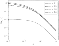
Figure S1: The function $\mathcal{I}(\epsilon_{v},\epsilon_{r})$ entering the Asimov likelihood profile in (15) for the Plummer sphere model. The parameters are $\epsilon_{v}=v_{0}/v_{\text{sh}}$ and $\epsilon_{r}=r_{s}/R$. Larger values of $\mathcal{I}(\epsilon_{v},\epsilon_{r})$ indicate better sensitivity to DM subhalos.

.3 6-D vs. 3-D kinematic data

In order to asses the advantage of using the full 6-D kinematic data, as opposed to 3-D information, we need to know the un-binned likelihood functions based on only the velocity or number density. They can be written analogously to (8):

$$\begin{split}p_{\text{velocity}}(d|{\mathcal{M}},{\bm{\theta}})&=\prod_{k=1}^{\bar{N}_{\text{star}}}\,\frac{f(\mathbf{x}_{k},\mathbf{v}_{k})({\mathbf{\theta}})}{n(\mathbf{x}_{k})(\mathbf{\theta})}\,,\end{split}$$ (S9)

and

$$\begin{split}p_{\text{number}}(d|{\mathcal{M}},{\bm{\theta}})&=e^{-N_{\text{star}}({\mathbf{\theta}})}\prod_{k=1}^{\bar{N}_{\text{star}}}\,n(\mathbf{x}_{k})({\mathbf{\theta}})\,,\end{split}$$ (S10)

where the data set $d$ is now restricted to $\{\mathbf{v}_{k}\}$ and $\{\mathbf{x}_{k}\}$, respectively.

We show an example of the Asimov likelihood profile, under the null hypothesis, comparing the 6-D and 3-D distributions in Fig. S2. We take $v_{0}\,=\,100\leavevmode\nobreak\ \text{km/s}$, $n_{0}\,=\,5\times 10^{3}\,\text{kpc}^{-3}$, $M_{sh}\,=\,2\times 10^{7}\,\text{M}_{\odot}$, $v_{\text{sh}}\,=\,200\leavevmode\nobreak\ \text{km/s}$, and ROI radius $R\,=\,3\leavevmode\nobreak\ \text{kpc}$. As shown in Fig S2, the likelihood profile using the full phase space information is not much different from that obtained with only velocity information. This indicates that one can work with the simplified likelihood function, which does not require a complete sample of stars, and obtain similar sensitivity to DM subhalos. On the other hand, the likelihood function that only uses the stellar number density data is significantly less sensitive, by almost one orders of magnitude in mass, to DM subhalos.

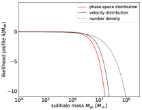
Figure S2: Likelihood profiles obtained using the Asimov dataset under the null hypothesis, with parameters as in Fig. 1, for the 6-D and 3-D likelihood functions.

References

- (1) V. Springel, J. Wang, M. Vogelsberger, A. Ludlow, A. Jenkins, A. Helmi, J. F. Navarro, C. S. Frenk, and S. D. M. White, The Aquarius Project: the subhalos of galactic halos, Mon. Not. Roy. Astron. Soc. 391 (2008) 1685–1711, [arXiv:0809.0898].
- (2) P. Colin, V. Avila-Reese, and O. Valenzuela, Substructure and halo density profiles in a warm dark matter cosmology, Astrophys. J. 542 (2000) 622–630, [astro-ph/0004115].
- (3) P. Bode, J. P. Ostriker, and N. Turok, Halo formation in warm dark matter models, Astrophys. J. 556 (2001) 93–107, [astro-ph/0010389].
- (4) M. Viel, J. Lesgourgues, M. G. Haehnelt, S. Matarrese, and A. Riotto, Constraining warm dark matter candidates including sterile neutrinos and light gravitinos with WMAP and the Lyman-alpha forest, Phys. Rev. D71 (2005) 063534, [astro-ph/0501562].
- (5) W. Hu, R. Barkana, and A. Gruzinov, Cold and fuzzy dark matter, Phys. Rev. Lett. 85 (2000) 1158–1161, [astro-ph/0003365].
- (6) B. Li, T. Rindler-Daller, and P. R. Shapiro, Cosmological Constraints on Bose-Einstein-Condensed Scalar Field Dark Matter, Phys. Rev. D89 (2014), no. 8 083536, [arXiv:1310.6061].
- (7) L. Hui, J. P. Ostriker, S. Tremaine, and E. Witten, Ultralight scalars as cosmological dark matter, Phys. Rev. D95 (2017), no. 4 043541, [arXiv:1610.08297].
- (8) D. N. Spergel and P. J. Steinhardt, Observational evidence for selfinteracting cold dark matter, Phys. Rev. Lett. 84 (2000) 3760–3763, [astro-ph/9909386].
- (9) B. D. Wandelt, R. Dave, G. R. Farrar, P. C. McGuire, D. N. Spergel, and P. J. Steinhardt, Selfinteracting dark matter, in Sources and detection of dark matter and dark energy in the universe. Proceedings, 4th International Symposium, DM 2000, Marina del Rey, USA, February 23-25, 2000, pp. 263–274, 2000. astro-ph/0006344.
- (10) M. Kaplinghat, S. Tulin, and H.-B. Yu, Self-interacting Dark Matter Benchmarks, arXiv:1308.0618.
- (11) M. A. C. Perryman, K. S. de Boer, G. Gilmore, E. Høg, M. G. Lattanzi, L. Lindegren, X. Luri, F. Mignard, O. Pace, and P. T. de Zeeuw, GAIA: Composition, formation and evolution of the Galaxy, A&A 369 (Apr., 2001) 339–363, [astro-ph/0101235].
- (12) LSST Science Collaboration, P. A. Abell, J. Allison, S. F. Anderson, J. R. Andrew, J. R. P. Angel, L. Armus, D. Arnett, S. J. Asztalos, T. S. Axelrod, et al., LSST Science Book, Version 2.0, arXiv:0912.0201.
- (13) The Dark Energy Survey Collaboration, The Dark Energy Survey, astro-ph/0510346.
- (14) SDSS Collaboration, M. Juric et al., The Milky Way Tomography with SDSS. 1. Stellar Number Density Distribution, Astrophys. J. 673 (2008) 864–914, [astro-ph/0510520].
- (15) R. Feldmann and D. Spolyar, Detecting Dark Matter Substructures around the Milky Way with Gaia, Mon. Not. Roy. Astron. Soc. 446 (2015) 1000–1012, [arXiv:1310.2243].
- (16) R. A. Ibata, G. F. Lewis, M. J. Irwin, and T. Quinn, Uncovering cold dark matter halo substructure with tidal streams, Mon. Not. Roy. Astron. Soc. 332 (June, 2002) 915–920, [astro-ph/0110690].
- (17) K. V. Johnston, D. N. Spergel, and C. Haydn, How Lumpy Is the Milky Way’s Dark Matter Halo?, ApJ 570 (May, 2002) 656–664, [astro-ph/0111196].
- (18) J. M. Siegal-Gaskins and M. Valluri, Signatures of LCDM substructure in tidal debris, Astrophys. J. 681 (2008) 40–52, [arXiv:0710.0385].
- (19) J. Bovy, Detecting the disruption of dark-matter halos with stellar streams, Phys. Rev. Lett. 116 (2016), no. 12 121301, [arXiv:1512.00452].
- (20) R. G. Carlberg, Modeling GD-1 Gaps in a Milky Way Potential, ApJ 820 (Mar., 2016) 45, [arXiv:1512.01620].
- (21) D. Erkal, V. Belokurov, J. Bovy, and J. L. Sanders, The number and size of subhalo-induced gaps in stellar streams, Mon. Not. Roy. Astron. Soc. 463 (Nov., 2016) 102–119, [arXiv:1606.04946].
- (22) D. Erkal, S. E. Koposov, and V. Belokurov, A sharper view of Pal 5’s tails: discovery of stream perturbations with a novel non-parametric technique, Mon. Not. Roy. Astron. Soc. 470 (Aug., 2017) 60–84, [arXiv:1609.01282].
- (23) S.-d. Mao and P. Schneider, Evidence for substructure in lens galaxies?, Mon. Not. Roy. Astron. Soc. 295 (1998) 587–594, [astro-ph/9707187].
- (24) Y. Hezaveh, N. Dalal, G. Holder, M. Kuhlen, D. Marrone, N. Murray, and J. Vieira, Dark Matter Substructure Detection Using Spatially Resolved Spectroscopy of Lensed Dusty Galaxies, Astrophys. J. 767 (Apr., 2013) 9, [arXiv:1210.4562].
- (25) Y. D. Hezaveh et al., Detection of lensing substructure using ALMA observations of the dusty galaxy SDP.81, Astrophys. J. 823 (2016), no. 1 37, [arXiv:1601.01388].
- (26) R. H. Brandenberger, N. Kaiser, and N. Turok, Dissipationless Clustering of Neutrinos Around a Cosmic String Loop, Phys. Rev. D36 (1987) 2242.
- (27) H. C. Plummer, On the problem of distribution in globular star clusters, Mon. Not. Roy. Astron. Soc. 71 (1911) 460–470.
- (28) J. F. Navarro, C. S. Frenk, and S. D. M. White, A Universal density profile from hierarchical clustering, Astrophys. J. 490 (1997) 493–508, [astro-ph/9611107].
- (29) J. Diemand, M. Kuhlen, P. Madau, M. Zemp, B. Moore, D. Potter, and J. Stadel, Clumps and streams in the local dark matter distribution, Nature 454 (2008) 735–738, [arXiv:0805.1244].
- (30) G. Cowan, K. Cranmer, E. Gross, and O. Vitells, Asymptotic formulae for likelihood-based tests of new physics, Eur. Phys. J. C71 (2011) 1554, [arXiv:1007.1727]. [Erratum: Eur. Phys. J.C73,2501(2013)].
- (31) D. Erkal and V. Belokurov, Properties of dark subhaloes from gaps in tidal streams, Mon. Not. Roy. Astron. Soc. 454 (Dec., 2015) 3542–3558, [arXiv:1507.05625].
- (32) C. Jordi, M. Gebran, J. M. Carrasco, J. de Bruijne, H. Voss, C. Fabricius, J. Knude, A. Vallenari, R. Kohley, and A. Mora, Gaia broad band photometry, A&A 523 (Nov., 2010) A48, [arXiv:1008.0815].
- (33) S. E. Koposov, G. Gilmore, M. G. Walker, V. Belokurov, N. Wyn Evans, M. Fellhauer, W. Gieren, D. Geisler, L. Monaco, J. E. Norris, S. Okamoto, J. Peñarrubia, M. Wilkinson, R. F. G. Wyse, and D. B. Zucker, Accurate Stellar Kinematics at Faint Magnitudes: Application to the Boötes I Dwarf Spheroidal Galaxy, Astrophys. J. 736 (Aug., 2011) 146, [arXiv:1105.4102].
- (34) G. Gilmore, S. Randich, M. Asplund, J. Binney, P. Bonifacio, J. Drew, S. Feltzing, A. Ferguson, R. Jeffries, G. Micela, et al., The Gaia-ESO Public Spectroscopic Survey, The Messenger 147 (Mar., 2012) 25–31.
- (35) G. D. et.al, WEAVE: the next generation wide-field spectroscopy facility for the William Herschel Telescope, 2012.
- (36) R. S. de Jong et al., 4MOST: the 4-metre Multi-Object Spectroscopic Telescope project at preliminary design review, 2016.
- (37) D. Hooper and S. J. Witte, Gamma Rays From Dark Matter Subhalos Revisited: Refining the Predictions and Constraints, JCAP 1704 (2017), no. 04 018, [arXiv:1610.07587].
- (38) S. Garrison-Kimmel, M. Boylan-Kolchin, J. Bullock, and K. Lee, ELVIS: Exploring the Local Volume in Simulations, Mon. Not. Roy. Astron. Soc. 438 (2014), no. 3 2578–2596, [arXiv:1310.6746].
- (39) G. Despali and S. Vegetti, The impact of baryonic physics on the subhalo mass function and implications for gravitational lensing, Mon. Not. Roy. Astron. Soc. 469 (2017) 1997, [arXiv:1608.06938].
- (40) T. Sawala, P. Pihajoki, P. H. Johansson, C. S. Frenk, J. F. Navarro, K. A. Oman, and S. D. M. White, Shaken and Stirred: The Milky Way’s Dark Substructures, Mon. Not. Roy. Astron. Soc. 467 (2017), no. 4 4383–4400, [arXiv:1609.01718].
- (41) R. Errani, J. Peñarrubia, C. F. P. Laporte, and F. A. Gómez, The effect of a disc on the population of cuspy and cored dark matter substructures in Milky Way-like galaxies, Mon. Not. Roy. Astron. Soc. 465 (Feb., 2017) L59–L63, [arXiv:1608.01849].
- (42) M. Lisanti, D. N. Spergel, and P. Madau, Signatures of Kinematic Substructure in the Galactic Stellar Halo, Astrophys. J. 807 (2015), no. 1 14, [arXiv:1410.2243].
- (43) G. Aslanyan, L. C. Price, J. Adams, T. Bringmann, H. A. Clark, R. Easther, G. F. Lewis, and P. Scott, Ultracompact minihalos as probes of inflationary cosmology, Phys. Rev. Lett. 117 (2016), no. 14 141102, [arXiv:1512.04597].