Gas-Phase Spectra of MgO Molecules: A Possible Connection from Gas-Phase Molecules to Planet Formation

Abstract

A more fine-tuned method for probing planet-forming regions, such as protoplanetary discs, could be rovibrational molecular spectroscopy observation of particular premineral molecules instead of more common but ultimately less related volatile organic compounds. Planets are created when grains aggregate, but how molecules form grains is an ongoing topic of discussion in astrophysics and planetary science. Using the spectroscopic data of molecules specifically involved in mineral formation could help to map regions where planet formation is believed to be occurring in order to examine the interplay between gas and dust. Four atoms are frequently associated with planetary formation: Fe, Si, Mg, and O. Magnesium, in particular, has been shown to be in higher relative abundance in planet-hosting stars. Magnesium oxide crystals comprise the mineral periclase making it the chemically simplest magnesium-bearing mineral and a natural choice for analysis. The monomer, dimer, and trimer forms of (MgO)_n with $n=1-3$ are analyzed in this work using high-level quantum chemical computations known to produce accurate results. Strong vibrational transitions at 12.5 $\mu$m, 15.0 $\mu$m, and 16.5 $\mu$m are indicative of magnesium oxide monomer, dimer, and trimer making these wavelengths of particular interest for the observation of protoplanetary discs and even potentially planet-forming regions around stars. If such transitions are observed in emission from the accretion discs or absorptions from stellar spectra, the beginning stages of mineral and, subsequently, rocky body formation could be indicated.

1 Introduction

The crossover in chemical classification from gaseous to solid matter is a difficult question to answer in terms of astrophysics and astrochemistry. The low pressures and various temperature extremes of diverse astrophysical environments often inhibit the creation of anything molecular beyond the gas phase. Yet, rocky bodies are comprised of solid matter. How and when a cluster of monomer molecules can begin to be classified as a mineral solid, especially with regards to those that comprise bodies such as rocky planets, is still not well understood (Gail & Sedlmayr, 1999; McWilliams et al., 2012). The main hang-up for this analysis is largely centered around what molecular species can be observed as indicators of changes in the region being observed and mapped.

Most of the interstellar molecules detected thus far have been gaseous and have atomic compositions from the upper-right of the periodic table (McCarthy & Thaddeus, 2001; Fortenberry, 2017) since carbon, nitrogen, and oxygen are among the most abundant elements in the universe (Savage & Sembach, 1996). While many of these have pertinence to planetary atmospheres, origins of life, and have even been detected in protoplanetary discs (Qi et al., 2003), few have been tied directly to the formation of geologically-related solids and their constituent minerals. As such, reason exists to shift toward the other side of the periodic table for searches related to rocky planets and how/where they might form. Most notably, [Al]/[Fe], [Si]/[Fe], [Sc]/[Fe], [Ti]/[Fe], and [Mg]/[Fe] ratios have been found to be statistically-significantly higher in the spectra of planet-hosting star systems (Adibekyan et al., 2012). Consequently, these atoms, are likely important in small-mass planet formation, and the higher [Mg]/[Si] ratio taken in the spectrum of a star or in that of a protoplanetary disc, the more likely planets are to be found (Adibekyan et al., 2015). Since magnesium is also one of the ten-most abundant atoms in the universe (Savage & Sembach, 1996) molecules containing magnesium should be fairly common. As a result, magnesium almost certainly plays a role in solid mineral and subsequent rocky body formation, and molecules containing it could be utilized as indicators of such processes.

Molecules containing one atom of magnesium have been previously detected in the interstellar medium (ISM). The carbon rich star IRC +10 216 has played host to a significant portion of the known, unique interstellar molecules, and those containing Mg are no exception. Notably, these include: HMgNC detected in 2013 (Cabezas et al., 2013), MgNC in 1993 (Kawaguchi et al., 1993), MgCN in 1995 (Ziurys et al., 1995), and MgCCH in 2014 (Agúndez, Cernicharo & Guélin, 2014). While these forms have been detected, there seems to be no direct tie between them and mineral formation.

Alternatively, the spectrum of the as-of-yet undetected magnesium oxide (MgO) clusters would be a natural place to begin such remote sensing. In addition to the abundance of magnesium, the presence of atomic oxygen in space is quite prevalent, as it is the third most abundant element in the universe (Savage & Sembach, 1996). Although the formation of an Mg$-$O bond is unlikely in hydrogen rich environments (Kohler, Gail & Sedlmayr, 1997), the formation of an ionic bond between oxygen and magnesium is inevitable due the atoms’ abundances and large electrostatic attraction.

Furthermore, on Earth, magnesium oxide is the chemically simplest mineral containing magnesium since it contains a repeating pattern of only two atoms. In its cubic form, magnesium oxide creates the mineral periclase. This mineral occurs naturally in contact metamorphic rocks and also in the form of ferropericlase (Fe,Mg)O in conjunction with iron making up about 20% of the Earth’s mantle (Ohta et al., 2017). Magnesium oxide has become well-known as a refractory material and is remarkably resistant to changes when put under extremely high temperatures and pressures (Koker, 2010). In its solid form, magnesium oxide is not magnetically conductive, but its superheated liquid-phase is magnetic (Coppari et al., 2013). This liquid-phase may exist as melt in the interiors of Super-Earths. Melt in terrestrial planet interiors can enable magnetic fields of the planet due to their electrically conductive characteristics (Coppari et al., 2013).

In order for planetary formation to occur, all minerals must form from molecules which must form from atoms in the gas-phase. These gas-phase molecules aggregate eventually to form planetesimals which mark the beginning of rocky planet formation (Pollack et al., 1996). To determine where these gas-phase molecules may be found and at what stage of planet formation they aggregate, highly accurate spectroscopic data are needed for increasingly larger numbers of MgO clusters. Delineations in column densities or local abundances observed in protoplanetary discs for the monomer would indicate gas phase chemistry, while increased presence of the dimer, trimer, and larger clusters would give a sign of a trend toward the solid and mineral phase, especially for spectral features for each larger molecular cluster. Such could be a marker for the initiation of mineral or solid material formation, but the unique features of each molecule must be available for reference.

Even though, the spectral features of magnesium oxide monomer were originally observed by Herzberg over 50 years ago (Herzberg, 1966), the dimer, trimer, and higher $n$-mers have been little studied save for some anion photodetachment analysis (Gutowski et al., 2000). The relative energies and structural data for the gaseous clusters of (MgO)_n ($n=1-40$), have been previously calculated with density functional theory (Chen, Xu & Zhang, 2008; Chen, Felmy & Dixon, 2014; Feitoza et al., 2017) showing patterns of aggregation. Most notably, the face-centered cubic patterns of (MgO)_n begin to emerge at $n=4$ as a cube built from two, stacked (MgO)₂ structures. However, depending upon the $n$ value, cubic and hexagonal isomers vie for the minimum energy structure (Chen, Felmy & Dixon, 2014). In any case, spectral data for the smallest of these clusters will assist in the characterization of magnesium oxide forms in the laboratory and potentially even in mapping the physical properties of protoplanetary discs.

2 Computational Details

In the current work, the necessary vibrational frequencies and rotational constants have been computed quantum chemically via a quartic force field, a fourth-order Taylor series expansion of the internuclear Hamiltonian (Fortenberry et al., 2013) and is of the form:

$$V=\frac{1}{2}\sum_{ij}F_{ij}\Delta_{i}\Delta_{j}+\frac{1}{6}\sum_{ijk}F_{ijk}\Delta_{i}\Delta_{j}\Delta_{K}+\frac{1}{24}\sum_{ijkl}F_{ijkl}\Delta_{i}\Delta_{j}\Delta_{k}\Delta_{l},$$ (1)

in which the $F_{ij\dots}$ represents the force constants and the $\Delta_{i}$ terms describe the displacements. In the past these types of calculations have produced vibrational fundamental frequencies to within as good as 1.0 cm^-1 and rotational constants within 50 MHz of experimental data (Fortenberry et al., 2011, 2012; Huang, Fortenberry & Lee, 2013; Zhao, Doney & Linnartz, 2014; Fortenberry et al., 2014a, b; Fortenberry, Lee & Müller, 2015; Morgan & Fortenberry, 2015a, b; Fortenberry, Roueff & Lee, 2016; Kitchens & Fortenberry, 2016; Bizzocchi et al., 2017). With these results, accurate rovibrational molecular spectra can be produced, such that small clusters of (MgO)_n can be detected.

Coupled cluster theory (Crawford & Schaefer III, 2000; Shavitt & Bartlett, 2009) at the singles, doubles, and perturbative triples [CCSD(T)] level (Raghavachari et al., 1989) as well as the explicitly correlated second-order Møller-Plesset perturbation theory MP2-F12 levels (Raghavachari et al., 1989; Møller & Plesset, 1934; Werner, Adler & Manby, 2007; Hill & Peterson, 2010) are utilized to determine the spectroscopic properties of the magnesium oxide clusters. The CCSD(T) method used to calculate the spectroscopic data in this work is regarded as the “gold standard” of quantum chemistry (Helgaker et al., 2004). The lower-level MP2 approach is significantly less costly than CCSD(T) which allows it to treat larger systems, such as the magnesium oxide trimer here. Additionally, MP2 is known to produce surprisingly accurate results for a relatively low level of theory due to the presence of a fortuitous cancellation of errors called a “Pauling point” in honor of Linus Pauling (Zheng, Zhao & Truhlar, 2009; Sherrill, 2009; Fink, 2016). The MOLPRO 2015.1 program (Werner et al., 2015, 2012) as well as the PSI4 program (Turney et al., 2012; Parrish et al., 2107) are used to perform the quantum chemical computations.

2.1 CCSD(T)-level Computations for MgO and (MgO)₂

In order to form a QFF for the closed shell molecules, MgO and (MgO)₂, a restricted Hartree-Fock CCSD(T)/aug-cc-pV5Z (Dunning, 1989; Kendall, Dunning & Harrison, 1992; Peterson & Dunning, 1995; Prascher et al., 2011) geometry optimization is performed to compute the initial geometry. The Martin-Taylor (MT) (Martin & Taylor, 1994) core correlating basis set is also used to modify the geometry to include core-orbitals, $1s$ for oxygen and $1s2s2p$ for magnesium. The reference geometries for these molecules are determined by combining the CCSD(T)/aug-cc-pV5Z optimized geometry and the differences in the CCSD(T)/MT optimized geometry with and without the core orbitals. This geometry optimization is performed in order to construct a structure which is as close as possible to the true minimum.

From the reference geometries, the energy points for the anharmonic internuclear potential, which subsequently is used to produce the spectroscopic data, are defined. The MgO monomer QFF requires 9 total points, and the (MgO)₂ QFF requires 233 total points. The displacements of these points, the $\Delta_{i}$ terms from Eq. 1, are described as 0.005 Å for bond length coordinates and 0.005 radians for all bond angles and torsions. The displacements are then used to define the Taylor series expansion and refine the true minimum energy structure.

Only one symmetry-internal coordinate defines the MgO molecule:

$$S_{1}(\sigma) =(\mathrm{O}-\mathrm{Mg}),$$ (2)

where the above coordinate is simply the distance between the oxygen and magnesium atoms. To fourth-order, there are four steps of positive displacements, four steps of negative displacements, and the reference mimum producing 9 total points. The dimer, (MgO)₂, requires 233 total points described by the following symmetry-internal coordinates:

$$S_{1}(a_{g}) =\frac{1}{\sqrt{2}}[(\mathrm{O}_{1}-\mathrm{O}_{2})+(\mathrm{Mg}_{1}-\mathrm{Mg}_{2})]$$ (3)

$$S_{2}(a_{g}) =\frac{1}{\sqrt{2}}[(\mathrm{O}_{1}-\mathrm{O}_{2})-(\mathrm{Mg}_{1}-\mathrm{Mg}_{2})]$$ (4)

$$S_{3}(b_{1g}) =\frac{1}{2}[(\mathrm{O}_{1}-\mathrm{Mg}_{1})-(\mathrm{O}_{1}-\mathrm{Mg}_{2})-(\mathrm{O}_{2}-\mathrm{Mg}_{1})+(\mathrm{O}_{2}-\mathrm{Mg}_{2})]$$ (5)

$$S_{4}(b_{1u}) =\tau[(\mathrm{O}_{1}-\mathrm{Mg}_{1}-\mathrm{O}_{2}-\mathrm{Mg}_{2})]$$ (6)

$$S_{5}(b_{3u}) =\frac{1}{2}[(\mathrm{O}_{1}-\mathrm{Mg}_{1})+(\mathrm{O}_{1}-\mathrm{Mg}_{2})-(\mathrm{O}_{2}-\mathrm{Mg}_{1})-(\mathrm{O}_{2}-\mathrm{Mg}_{2})]$$ (7)

$$S_{6}(b_{2u}) =\frac{1}{2}[(\mathrm{O}_{1}-\mathrm{Mg}_{1})-(\mathrm{O}_{1}-\mathrm{Mg}_{2})+(\mathrm{O}_{2}-\mathrm{Mg}_{1})-(\mathrm{O}_{2}-\mathrm{Mg}_{2})],$$ (8)

where the atom numbers are given in Figure 1.

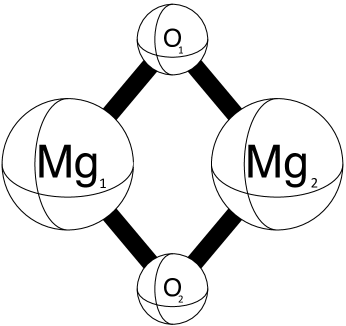
Figure 1: The CcCR Optimized Geometry of Planar, $D_{2h}$ (MgO)₂.

At each point, the energy produced is determined from CCSD(T). Using the aug-cc-pVTZ, aug-cc-pVQZ, and aug-cc-pV5Z basis sets, the CCSD(T) energy can be extrapolated using a three-point complete basis set (CBS) limit (Martin & Lee, 1996). The energy differences between the CCSD(T) computations retaining core orbitals and those lacking core orbitals again utilizing the MT basis set are added to the CCSD(T)/CBS energies. Additionally, the scalar relativistic (Douglas & Kroll, 1974) corrections are also added from computations utilizing the cc-pVTZ-DK basis set for relativity included and excluded. Using these techniques to compute exceedingly accurate energies is defined as the CcCR QFF (Huang & Lee, 2008, 2009; Huang, Taylor & Lee, 2011; Fortenberry et al., 2011). The “C” represents the CBS energy, the “cC” represents the core correlation calculated as the difference between the MT and MTc energies, and the “R” represents scalar relativity. As mentioned above, these CcCR QFF computations are highly accurate models that can physically describe spectroscopic data.

2.2 MP2-F12 for (MgO)₂ and (MgO)₃

The methodology for the MP2-F12 level has congruencies with the CCSD(T) level. To begin, the initial geometry is optimized using the MP2-F12/aug-cc-pVDZ. This optimized geometry is then used to define the necessary energy points to form the anharmonic potential. Again, the (MgO)₂ QFF requires 233 total energy points, but the (MgO)₃ QFF requires 3789 total energy points. The displacements are still 0.005 Å for bond length coordinates and 0.005 radians for all bond angles and torsions. The coordinates for the dimer are the same as those defined above for the CcCR QFF. The trimer, (MgO)₃, is of $D_{3h}$ symmetry, but will be run in $C_{2v}$ for ease in constructing the points and in the force constants analysis. The magnesium oxide trimer’s QFF is defined by 12 symmetry-internal coordinates:

$$S_{1}(a_{1}) =\frac{1}{\sqrt{2}}[(\mathrm{Mg}_{1}-\mathrm{O}_{2})+(\mathrm{Mg}_{1}-\mathrm{O}_{3})]$$ (9)

$$S_{2}(a_{1}) =\frac{1}{\sqrt{2}}[(\mathrm{Mg}_{1}-\mathrm{Mg}_{2})+(\mathrm{Mg}_{1}-\mathrm{Mg}_{3})]$$ (10)

$$S_{3}(a_{1}) =(\mathrm{Mg}_{1}-\mathrm{O}_{1})$$ (11)

$$S_{4}(a_{1}) =\frac{1}{\sqrt{2}}[(\mathrm{O}_{2}-\mathrm{Mg}_{1}-\mathrm{Mg}_{2})+(\mathrm{O}_{3}-\mathrm{Mg}_{1}-\mathrm{Mg}_{3})]$$ (12)

$$S_{5}(a_{1}) =\frac{1}{\sqrt{2}}[(\mathrm{O}_{2}-\mathrm{Mg}_{1}-\mathrm{O}_{1})+(\mathrm{O}_{3}-\mathrm{Mg}_{1}-\mathrm{O}_{1})]$$ (13)

$$S_{6}(b_{2}) =\frac{1}{\sqrt{2}}[(\mathrm{Mg}_{1}-\mathrm{O}_{2})-(\mathrm{Mg}_{1}-\mathrm{O}_{3})]$$ (14)

$$S_{7}(b_{2}) =\frac{1}{\sqrt{2}}[(\mathrm{Mg}_{1}-\mathrm{Mg}_{2})-(\mathrm{Mg}_{1}-\mathrm{Mg}_{3})]$$ (15)

$$S_{8}(b_{2}) =\frac{1}{\sqrt{2}}[\angle(\mathrm{O}_{2}-\mathrm{Mg}_{1}-\mathrm{Mg}_{2})-\angle(\mathrm{O}_{3}-\mathrm{Mg}_{1}-\mathrm{Mg}_{3})]$$ (16)

$$S_{9}(b_{2}) =\frac{1}{\sqrt{2}}[(\mathrm{O}_{2}-\mathrm{Mg}_{1}-\mathrm{O}_{1})-(\mathrm{O}_{3}-\mathrm{Mg}_{1}-\mathrm{O}_{1})]$$ (17)

$$S_{10/x}(b_{1}) =\frac{1}{\sqrt{2}}\tau[(\mathrm{O}_{3}-\mathrm{Mg}_{1}-\mathrm{Mg}_{3}-\mathrm{O}_{1})-(\mathrm{O}_{2}-\mathrm{Mg}_{1}-\mathrm{Mg}_{2}-\mathrm{O}_{1})]$$ (18)

$$S_{11/y}(b_{1}) =\tau(\mathrm{O}_{2}-\mathrm{Mg}_{1}-\mathrm{O}_{3}-\mathrm{O}_{1})$$ (19)

$$S_{12/z}(a_{2}) =\frac{1}{\sqrt{2}}\tau[(\mathrm{O}_{3}-\mathrm{Mg}_{1}-\mathrm{Mg}_{3}-\mathrm{O}_{1})+(\mathrm{O}_{2}-\mathrm{Mg}_{1}-\mathrm{Mg}_{2}-\mathrm{O}_{1})].$$ (20)

At each point, MP2-F12/aug-cc-pVDZ energies are computed, and this QFF is only defined by these terms. The atom labels are shown in Figure 2.

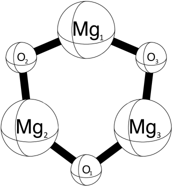
Figure 2: The MP2-F12/aug-cc-pVDZ Optimized Geometry of Planar, $D_{3h}$ (MgO)₃.

2.3 Forming the QFF with CCSD(T) and MP2-F12 methods

After obtaining the set of energies, the QFF is fitted. A least-squares fitting of the energy points (whether CcCR or MP2-F12) produces results with minimal error as indicated by the sum of squared residuals of less than 10^-16 a.u.² (10^-18 for the monomer and dimer) for all levels of theory used and molecules examined. This fitting produces the equilibrium geometry. Refitting once more zeroes the gradients and produces the force constants needed to define the potential portion for the internuclear Hamiltonian, the QFF (Eq. 1).

The INTDER (Allen & coworkers, 2005) program transforms the computed force constants into Cartesian coordinates which are more readily translated for subsequent generic analysis. Rotational and vibrational second-order perturbation theory (VPT2) (Mills, 1972; Watson, 1977; Papousek & Aliev, 1982) are employed by combining the previously computed potential energy and the new kinetic energy via the SPECTRO (Gaw et al., 1991) program. These analyses provide the anharmonic vibrational frequencies and spectroscopic data. (MgO)₂ possesses a $2\nu_{6}=\nu_{1}$ type-1 Fermi resonance as well as $\nu_{3}/\nu_{2}$ and $\nu_{5}/\nu_{4}$ C$-$type Coriolis resonances. (MgO)₃ exhibits dozens of type-1 and type-2 Fermi, Coriolis, and Darling-Denison resonances, but none perturb the vibrational frequencies by more than 2 cm^-1 which is well within the expected accuracy of MP2-F12/aug-cc-pVDZ approach utilized here. All vibrational intensities are computed within the double-harmonic approximation and with MP2/6-31+G^∗ in the Gaussian09 program (Møller & Plesset, 1934; Frisch et al., 2009; Hehre, Ditchfeld & Pople, 1972). This approximation has been shown to be in good agreement with higher-level computations for the prediciton of such properties (Fortenberry et al., 2014c; Yu et al., 2015).

3 Results and Discussion

3.1 MgO Singlet and Triplet

Table 1: The MgO CcCR Force Constants in mdyn/Åⁿ for $n,m=0,1,2,3,4$.

$\tilde{X}\ ^{1}\Sigma^{+}$ MgO		$A\ ^{3}\Pi$ MgO
F11	3.763 052	F11	2.384 934
F111	-22.118 502	F111	-11.858 582
F1111	66.966 674	F1111	52.025 584

Table 2: The MgO Singlet and MgO Triplet CcCR QFF VPT2 Bond Lengths, Spectroscopic Constants, and Vibrational Frequencies (with intensities in km/mol in parentheses)

		$\tilde{X}\ ^{1}\Sigma^{+}$ MgO					$A\ ^{3}\Pi$ MgO
		MgO	25MgO	26MgO	Mass Avg.	Experimenta	Mass Avg.	Experimentb
$r_{e}$ (O-Mg)	Å	1.738 981	–	–	–	1.7490	1.876 550	1.869 286
$B_{e}$	MHz	17416.0	17136.9	16880.3	17329.2	–	14881.5	–
Est. $B_{0}$	MHz				17242.5	17233.31	14807.1	15072.5
$D_{e}$	kHz	35.331	34.208	33.191	35.005	36.937	34.9574	35.92
$H_{e}$	mHz	-29.838	-28.426	-27.268	-29.440	–	-8.933	–
$\omega_{1}$	cm-1	814.8 (1127)	809.3	803.2	813.0	785.2	647.9 (61)	650.223

^a Irikura (2007) with $D$ from Mürtz et al. (1995).
^b Mürtz et al. (1995).

In order to determine accurate rovibrational spectroscopic data for (MgO)_n as a potential marker of mineral formation in protoplanetary discs, the analysis begins with the monomer, MgO. The CcCR symmetry-internal harmonic force constants for $\tilde{X}\ ^{1}\Sigma^{+}$ MgO and $A\ ^{3}\Pi$ MgO are listed in Table 1, and define the QFF. The singlet is more tightly bound in the F₁₁ value indicating a higher bond order. Magnesium is less inclined to form double bonds because this atom has a [Ne]$3s^{2}$ electron configuration. Sharing or outright removal of those $s$ orbitals are much more likely than any notable $p$ orbital population, which is a characteristic of a double bond. In fact, the triplet has a strength of merely 63% to that of the singlet. The implication is that $\tilde{X}\ ^{1}\Sigma^{+}$ MgO is more ionic in character since one of the electrons from the magnesium atom now occupies a lone pair orbital on the carbon in order to create the spin-pairing of the singlet. This relationship is somewhat unexpected since it is opposite of that noted for the isoelectronic MgCH₂ molecule recently analyzed in our group where the triplet state is the ground state (Bare et al., 2000; Bassett & Fortenberry, 2017). However, this has been known in MgO for over 40 years (Ikeda et al., 1977) and the more contemporary 2551.9713 cm^-1 $a^{3}\Pi\leftarrow\tilde{X}^{1}\Sigma^{+}$ transition frequency (Mürtz et al., 1994, 1995) is very close to the 2385 cm^-1 CcCR adiabatic excitation computed here. Regardless, MgO monomer will almost exclusively exist in the $\tilde{X}\ ^{1}\Sigma^{+}$ state in protoplanetary discs at distances where rocky planets will form since the excitation energy is equivalent to an ambient temperature of roughly 3700 K.

The CcCR QFF VPT2 bond lengths and spectroscopic constants are displayed in Table 2. The O$-$Mg bond is longer in the triplet state than in the singlet state as a result of the smaller F₁₁ value in the triplet. While $\tilde{X}\ ^{1}\Sigma^{+}$ MgO is more ionic than $A\ ^{3}\Pi$ MgO, the monomer can be more tightly bound since both electrons can be involved in the bonding. However, in the triplet, the electron is reatined by the magnesium but lies on the side opposite the carbon. Therefore, it is unavilable for bonding weaking the Mg$-$O interaction. The $\tilde{X}\ ^{1}\Sigma^{+}$ MgO bond length is comparable to the experimental bond length of 1.7490 Å (Irikura, 2007), and even the excited triplet state is within 0.02 Å of experiment at 1.869 286 Å (Mürtz et al., 1995). The variance in the bond lengths, rotational constants, and sextic distortion constants between the singlet and triplet states showcases that these two forms of MgO will be easily distinguished rotationally as well as electronically or by ambient temperature.

However, the computed rotational constant for $\tilde{X}\ ^{1}\Sigma^{+}$ MgO does not match that from experiment 17233.31 MHz (Irikura, 2007). Magnesium has three major isotopes, unlike oxygen, carbon, and hydrogen where one dominates. ²⁴Mg has a natural abundance of 79%, ²⁵Mg is 10%, and ²⁶Mg is 11%. By averaging the equilibrium rotational constants, $B_{e}$, for each isotopologue, 17329.2 MHz is produced, in much better agreement. Full vibrational-averaging for diatomics is problematic for the available software. However, estimates in the perturbation between $B_{e}$ and the more experimentally-meaningful $B_{0}$ values from data taken below for (MgO)₂ give a rotational constant within 10 MHz of experiment at 17242.5 MHz. Hence, our experimental methods should be similarly accurate for the dimer species below. Case in point are the quartic distortion contants ($D$) where is computed to be 35.004 kHz and experiment which is 36.937 kHz (Mürtz et al., 1995). The $A\ ^{3}\Pi$ bond length, rotational constant, $D$ value, and even vibrational frequecny are in excellent agreement with experiment (Mürtz et al., 1995) showcasing the accuracy of this computational approach.

The vibrational frequencies of MgO are also listed in Table 2. The singlet state has an incredibly bright intensity (1127 km/mol) for the fundamental mode due to an active charge transfer which is a hallmark of ionic species. Again, anharmonic computations are problematic for diatomics, but mass-averaging lowers the $\omega_{1}$ fundamental frequency somewhat to 813.0 cm^-1. Considering an anharmonic effect on the order of 10-20 cm^-1 puts the estimated frequency within 10 cm^-1 of the experimentally-observed value at 785.2 cm^-1. Consequently, any computational studies of magnesium must involve all three major isotopes in order for meaningful comparison to be had for physically observable properties whether in planet-forming regions or in the laboratory.

3.2 (MgO)₂

The dimer, (MgO)₂, requires significantly more force constants than the monomer. These force constants are produced in Table 1 of the Supporting Information (SI). The higher $D_{2h}$ symmetry means that the bond strengths arise from linear combinations of the force constants. As a result, the bonding in (MgO)₂ is somewhat weaker between individual Mg$-$O bonds, but the cross-bonding between like atoms in the ring and the cyclic stabilization create a more stable structure once two MgO pieces are brought together. In fact, the CcCR separation energy for (MgO)₂ $\rightarrow$ 2 MgO is -132.0 kcal/mol indicating a strong stabilization for creation of the dimer from the monomer. Granted some barrier will likely be present in any such reaction, but the thermodynamics will ultimately lead to the larger clusters. Each MgO unit contains 20 electrons meaning that each successive $n$-mer will be add a factor of 20 electrons to the system making for simple addition.

The vibrational frequencies of (MgO)₂ are shown in Table 3. The anharmonic corrections are well-behaved within our tight fitting giving no reason to doubt the accuracy of these values as within the 10 cm^-1 or less range established for MgO above and previously for $p$-block molecules. The mass averaging is of supreme importance here for observations of molecules mixed through a bulk. While the (²⁴MgO)₂ isotopologue will make up 62% of the observable amount of (MgO)₂, ²⁴MgO²⁵MgO and ²⁴MgO²⁶MgO will comprise 7.9% and 8.7% of (MgO)₂. Hence, these and the three other combinations of magnesium masses are included in the averaged values given in the furthest column of Table 3.

Only three of the six fundamental vibrational frequencies are infrared-active due to symmetry, $\nu_{2}$ (the oxygen atom translation), $\nu_{3}$ (the magnesium atom translation), and $\nu_{6}$ (the out-of-plane “book” motion) as given in Table 3. These three are all notably bright frequencies with intensities above 100 km/mol. Most molecules have intensities around a few dozen km/mol. As a result, the magnesium oxide dimer should be detectable even in reduced amounts as a consequence of Beer’s law. The 15-17 $\mu$m region at the beginning of the far-IR and approaching the THz region is well within the range of the James Webb Space Telescope (JWST) making this upcoming observatory a natural choice for future observation of the $\nu_{2}$ fundamental vibrational frequency of (MgO)₂. The 281.4 cm^-1 (35.5 $\mu$m or 8.44 THz) out-of-plane motion will be below what JWST can observe, but this is the least bright fundamental of the three. The frequencies for the two-quanta overtones for each of these fundamentals are also given in Table 3.

The differences between the CcCR and MP2-F12/aug-cc-pVDZ calculations differ by 3-5%. Hence, MP2-F12/aug-cc-pVDZ is well-behaved, but undershoots the prediction of the frequencies by as much as 30 cm^-1. However, this is close enough use in conjunction with isolated laboratory experiments for larger molecules where such anharmonic computations cannot be undertaken with the CcCR QFF.

Even though, (MgO)₂ is non-polar, the CcCR QFF structures and spectroscopic constants are included in Table 4 for completeness. The vibrationally-averaged ($R_{\alpha}$) bond lengths for (MgO)₂ differ slightly between the CcCR and MP2-F12/aug-cc-pVDZ methods as expected for different methods and basis sets. However, the spectroscopic $D$ and $H$ constants are consistent between the two approaches with the primary rotational constants roughly similar. The near-oblate nature of this molecule means that the $A$ and $B$ constants are closer to one another in magnitude and greater than the $C$. Even without a permanent dipole moment, rotational transitions of vibrationally-excited states of molecules have been detected in the ISM (Turner, 1987; Cernicharo et al., 2008) making the present predictions for the $A$, $B$, and $C$ constants of the 2, 3, and 6 states potentially of value for observations with the Atacama Large Millimeter Array (ALMA).

3.3 (MgO)₃

Creating the magnesium oxide trimer from three monomers will also produce 268.0 kcal/mol indicating that the trimer is even more stable than the dimer since half of this stabilization energy is 134.0 kcal/mol, 2.0 kcal/mol more than the dimer. Even though the two are computed with different methods (MP2-F12/aug-cc-pVDZ versus CcCR), the relative energies are still directly comparable. The slightly larger harmonic, diagonal (MgO)₃ force constants, displayed in Table 2 of the SI, also corroborate the growth in stabilization for larger clusters of (MgO)_n. Since periclase or bulk magnesium oxide is a stable ionic lattice, such an increase in stabilization for larger clusters is fully expected. As a result, the larger clusters are behaving more like the mineral with each addition of a monomer unit (Chen, Felmy & Dixon, 2014).

While there are 10 possible combinations of magnesium isotopes possible in (MgO)₃, only the six that contain at least one ²⁴Mg will have natural abundances of greater than 0.4%. Hence, the isotopes included in Tables 5 and 6 will make up more than 98% of any observable (MgO)₃. Only these are included in the mass averaging.

Of the twelve total fundamental vibrational frequencies, four are in degenerate pairs making a total of eight fundamental frequencies. Even though the QFF is computed in the lower-symmetry $C_{2v}$ point group, the vibrational frequencies are computed in full $D_{3h}$. Of the eight fundamental frequencies, four are vibrationally-active, but the $\nu_{3}$ motion is nearly unobservable. As a result and like with (MgO)₂, the magnesium oxide trimer has three observable fundamental vibrational frequencies (with atom labels from Fig. 2): $\nu_{2}(E^{\prime})$, the Mg₂+Mg₃/O₂+O₃ stretch akin to the vibrationally-active mode in H₃⁺; $\nu_{6}(A_{2}^{\prime\prime})$, the Mg triangle and O triangle out-of-plane separation; and $\nu_{7}(E^{\prime})$, the Mg₁+O₁ stretch).

The anharmonic shifts are small for the first four fundamentals. After that, the anharmonicities are fairly large and actually increase the fundamental frequency. Such behavior is not typical but not uncommon. These modes are low-frequency in the same range where most positive anharmonicities are reported in other highly-symmetric systems. However, $\nu_{5}-\nu_{8}$ should still be viewed as less trustworthy than the typically-behaving fundamentals in $\nu_{1}$-$\nu_{4}$. Follow-up experiments should be able to determine the $\nu_{6}$ and $\nu_{7}$ peak positions due to the large intensities of these motions. Regardless, these frequencies are not observable with JWST anyway.

The only observable fundamental frequency for (MgO)₃ in JWST’s range is $\nu_{7}$ which VPT2 with the MP2-F12/aug-cc-pVDZ QFF reports the mass averaged fundamental to be at 748.6 cm^-1. Taking the benchmark for the performance of the dimer and upscaling this value by 5% to perform more like the CcCR QFF puts the fundamental for this bright transition at roughly 785 cm^-1, 12.7$\mu$m, or 23.5 THz. This is in the exact range as the MgO monomer. Hence, their vibrational spectra will likely rest at nearly the same frequency.

According to Table 6 the mass averaged bond length in this molecule is 1.848 Å, shorter than the 1.860 Å mass averaged bond length in (MgO)₂ giving further indication of stronger bonding as discussed previously. This bond length does not vary significantly as the molecule includes the ²⁵Mg and ²⁶Mg isotopes such that the standard isotopologue and the other masses have the same structure for all intents and purposes. As with the dimer, (MgO)₃ has no dipole moment and will not be rotationally-observable. However, the rotational constants and spectroscopic data are provided for completeness. Magnesium oxide trimer is even more nearly-oblate than dimer as implied by the rotational constants and as expected by the structure. Again, the rotational spectra of some of the vibrationally-excited states could be observed. The accuracies for such data with MP2-F12/aug-cc-pVDZ would not be as good as desired, but the pure ground vibrational state rotational data should be a good first-order approximation for their values.

4 Conclusions

Since magnesium is known to be in higher relative abundances in stars that host planets and magnesium is believed to comprise a significant portion of terrestrial-type planets, molecules containing element-12 could serve as sentinel markers in planet forming regions where gas phase-chemistry is giving way to the creation of solids, minerals most notably. The simplest magnesium mineral, magnesium oxide or periclase, is a good place to begin such analysis. The advent of JWST will bring high-resolution to the observation of protoplanetary discs and planet forming regions around stars. This work provides data for the detection of the (MgO)_n molecular clusters for $n=1-3$. Such molecules are the building blocks of larger magnesium oxide crystals. Hence, if the $n\geq 2$ molecular clusters can be detected in the gas-phase in such planet-forming environments as protoplanetary discs, they will be clear indicators of larger mineral formation moving from the gas- to solid- (mineral) phases.

This work has shown that magnesium oxide clusters are more strongly bound as monomer units are added. Such is expected for premineral molecules that ultimately build larger clusters and eventually ionic lattices in solid materials. Additionally, the excellent monomer CcCR QFF benchmarks show that the equivalently computed dimer spectral features should be equivalently accurate. Therefore, scaling-up the trimer MP2-F12/aug-cc-pVDZ results will provide similar results, especially for the higher-frequency fundamentals.

In general, transitions at 12.5 $\mu$m (monomer & trimer), 15.0 $\mu$m (dimer), and 16.5 $\mu$m (dimer) will be clear indicators of initial periclase formation from these MgO clusters. These transitions also fall within a relatively clear window of observed spectra for known protoplanetary discs (Williams & Cieza, 2011). They are to the red of a dominant silicate feature at 10 $\mu$m making these peaks observable as shoulders or simply separate, lower-frequency peaks especially if the resolving power of JWST can be brought to bear. Since the 785 cm^-1/12.5 $\mu$m band is exhibited for both the monomer and the trimer, the tetramer will likely have a transition very close to this range. As a result, mapping the 12.5 $\mu$m band in protoplanetary discs while also mapping the growth of the dimer’s 16.5 $\mu$m band and/or the reduction in the monomer’s rotational signal could be indicators of the very first stages of where magnesium oxide turns from a gas into a proto-mineral. Consequently, the provided spectral features may allow for detailed and fine-tuned analysis of planet-forming regions and specifically protoplanetary discs.

5 Acknowledgements

RCF wishes to acknowledge NASA grant NNX17AH15G for support of this work. Additionally, the authors greatly acknowledge the support of the National Science Foundation (Award Number: NSF-CHE (REU) 1359229).

Table 3: The (MgO)₂ CcCR and MP2-F12/aug-cc-pVDZ QFF VPT2 Frequencies (in cm^-1) with MP2/6-31+G^∗ Double Harmonic Intensities (in km/mol in Parentheses).

Units	CcCR	MP2-F12	24Mg25Mg	25Mg 25Mg	25Mg 26Mg	26Mg 26Mg	24Mg26Mg	Mass Average
$\omega_{1}(A_{g})$	681.8	650.1	679.4	676.6	674.4	672.1	677.2	673.1
$\omega_{2}(B_{2u})$	673.6 (179)	641.1	671.0	668.2	665.7	663.2	668.7	664.5
$\omega_{3}(B_{3u})$	615.0 (201)	593.1	612.4	610.0	607.7	605.4	610.0	607.7
$\omega_{4}(B_{1g})$	580.7	558.8	577.8	575.0	572.3	569.8	574.9	572.8
$\omega_{5}(A_{g})$	453.4	441.7	450.5	447.6	444.7	441.9	447.6	446.8
$\omega_{6}(B_{1u})$	286.9 (141)	278.6	285.7	284.5	283.5	282.4	284.6	283.7
$\nu_{1}(A_{g})$	672.2	641.2	669.7	667.2	665.1	662.8	667.7	663.7
$\nu_{2}(B_{2u})$	661.8	630.4	659.3	656.6	654.3	651.8	657.1	653.1
$\nu_{3}(B_{3u})$	605.0	583.2	602.5	600.2	597.9	559.4	563.8	587.4
$\nu_{4}(B_{1g})$	569.4	548.1	566.5	563.9	561.3	558.8	563.8	561.7
$\nu_{5}(A_{g})$	450.3	439.0	447.4	444.6	441.7	438.9	444.6	443.8
$\nu_{6}(B_{1u})$	284.4	276.7	283.2	282.1	281.1	280.0	282.2	281.4
$2\nu_{2}$	1320.4	1257.8	1315.3	1197.1	1248.7	930.3	1310.9	1225.8
$2\nu_{3}$	1206.7	1163.1	1201.8	1310.0	1192.6	1149.4	1197.1	1202.9
$2\nu_{6}$	568.2	553.1	565.9	563.6	561.5	559.4	563.8	562.2
Zero-Point	1639.14	1575.90	1631.88				1625.13

Table 4: The CcCR QFF Zero-Point ($R_{\alpha}$ vibrationally-averaged) and Equilibrium Structures, Rotational Constants, and Quartic and Sextic Distortion Constants of (MgO)₂ and for the ²⁵Mg and ²⁶Mg Isotopologues.

	Units	CcCR	MP2-F12	24Mg25Mg	25Mg 25Mg	25Mg 26Mg	26Mg 26Mg	24Mg 26Mg	Mass Average
r0(O$-$Mg)		1.859944	1.88708	1.859905	1.859893	1.859883	1.859846	1.859867	1.859890
$\angle$(Mg$-$O$-$Mg)		79.999	79.918	79.998	79.999	79.999	79.998	79.997	79.998
$A_{0}$	MHz	7796.0	7564.7	7796.1	7796.3	7796.4	7796.5	7796.3	7796.3
$B_{0}$	MHz	7384.9	7186.1	7235.9	7089.4	6952.5	6817.6	7096.8	7096.2
$C_{0}$	MHz	3787.4	3680.4	3747.9	3708.2	3670.4	3632.5	3710.2	3709.4
$A_{1}$	MHz	7776.9	7544.8	7777.2	7777.6	7777.9	7778.3	7777.5	7777.6
$B_{1}$	MHz	7369.1	7170.9	7220.5	7074.2	6937.7	6803.1	7081.9	7081.1
$C_{1}$	MHz	3779.0	3671.9	3740.0	3700.2	3662.9	3624.9	3703.4	3701.7
$A_{2}$	MHz	7796.2	7563.4	7796.5	7796.9	7797.2	7797.5	7796.8	7796.9
$B_{2}$	MHz	7355.9	7158.8	7207.7	7061.8	6925.6	6791.3	7069.4	7068.6
$C_{2}$	MHz	3774.3	3667.3	3734.6	3695.3	3657.5	3620.0	3696.3	3696.3
$A_{3}$	MHz	7761.3	7530.5	7761.7	7761.9	7762.2	7762.4	7762.1	7761.9
$B_{3}$	MHz	7403.0	7203.7	7253.2	7106.0	6968.4	6833.0	7113.3	7112.8
$C_{3}$	MHz	3777.5	3670.5	3738.2	3698.7	3661.1	3623.4	3700.7	3699.9
$A_{4}$	MHz	7770.3	7538.9	7770.6	7770.8	7771.0	7771.1	7770.9	7770.8
$B_{4}$	MHz	7376.2	7177.4	7227.4	7081.2	6944.5	6809.9	7088.5	7088.0
$C_{4}$	MHz	3773.7	3666.8	3734.3	3694.7	3657.1	3619.3	3696.7	3696.0
$A_{5}$	MHz	7811.9	7580.8	7811.8	7811.8	7811.7	7811.6	7811.7	7811.8
$B_{5}$	MHz	7384.9	7185.0	7236.0	7089.5	6952.6	6817.8	7097.0	7096.3
$C_{5}$	MHz	3784.9	3677.8	3745.3	3705.7	3667.9	3630.0	3707.7	3706.9
$A_{6}$	MHz	7780.4	7548.8	7780.4	7780.3	7811.7	7811.6	7780.3	7790.8
$B_{6}$	MHz	7361.2	7162.3	7213.2	7067.5	6952.6	6817.8	7074.9	7081.2
$C_{6}$	MHz	3791.0	3683.7	3751.4	3711.6	3667.9	3630.0	3713.6	3710.9
re(O$-$Mg)	Å	1.853962	1.880792	1.853962	1.853962	1.853962	1.853962	1.853962	1.853962
$\angle$(Mg$-$O$-$Mg)	∘	80.026	79.951	80.026	80.026	80.026	80.026	80.026	80.026
$A_{e}$	MHz	7835.43	7605.11	7835.43	7835.43	7835.43	7835.43	7835.43	7835.43
$B_{e}$	MHz	7414.35	7215.57	7264.66	7117.37	6979.82	6844.33	7124.89	7124.24
$C_{e}$	MHz	3809.54	3702.61	3769.63	3729.58	3691.46	3653.21	3731.64	3730.84
$D_{J}$	kHz	3.296	3.1755	3.1542	3.0201	2.9003	2.7862	3.028	3.0308
$D_{JK}$	kHz	-3.1362	-2.6168	-2.8306	-2.559	-2.3299	2.7862	-2.5735	-1.7738
$D_{K}$	kHz	6.6563	6.2184	6.4924	6.355	6.2456	6.154	6.3615	6.3775
$d_{1}$	kHz	-1.6033	-1.5492	-1.5363	-1.4714	-1.4123	-1.355	-1.4753	-1.4756
$d_{2}$	kHz	-0.226	-0.2331	-0.2253	-0.2229	-0.2195	-1.355	-0.2231	-0.4120
$H_{J}$	Hz	0.00664	0.0062	0.00604	0.00549	0.00503	0.00461	0.00552	0.00556
$H_{JK}$	Hz	-0.0302	-0.02713	-0.02683	-0.02386	-0.02142	-0.01925	-0.02407	-0.02427
$H_{KJ}$	Hz	0.00459	-0.00095	0.00122	-0.00165	-0.00387	-0.00577	-0.00141	-0.00115
$H_{K}$	Hz	0.03331	0.0362	0.03392	0.03437	0.03461	0.03476	0.0343	0.0342
$h_{1}$	Hz	0.003	0.00284	0.00282	0.00266	0.00251	0.00236	0.00267	0.00267
$h_{2}$	Hz	-0.00013	-0.00011	-0.00001	0.00008	0.00015	0.00021	0.00008	0.00006
$h_{3}$	Hz	0.0002	0.00016	0.00018	0.00017	0.00016	0.00015	0.00017	0.00017

Table 5: The MP2-F12/aug-cc-pVDZ QFF VPT2 Magnesium Oxide Timer Frequencies (in cm^-1) with MP2/6-31+G^∗ Double Harmonic Intensities (in km/mol in Parentheses).

Units	24Mg24Mg24Mg	24Mg24Mg25Mg	24Mg 25Mg 25Mg	24Mg 26Mg 26Mg	24Mg 24Mg 26Mg	26Mg 24Mg 25Mg	Mass Average
$\omega_{1}(A_{2}^{\prime})$	782.3	780.2	777.8	774.6	778.9	776.3	778.3
$\omega_{2}(E^{\prime})$	757.6 (321)	757.4	754.6	751.0	757.1	753.7	755.2
		753.0	751.2	745.4	748.3	747.4	749.1
$\omega_{3}(E^{\prime})$	600.9 (1)	599.7	598.3	595.9	598.6	597.2	598.4
		599.4	598.1	595.5	598.0	596.7	597.5
$\omega_{4}(A_{1}^{\prime})$	513.3	512.6	511.8	510.5	511.9	511.1	511.9
$\omega_{5}(A_{1}^{\prime})$	355.0	353.1	351.2	347.7	351.3	349.5	351.3
$\omega_{6}(A_{2}^{\prime\prime})$	269.2 (220)	268.4	267.7	266.4	267.8	267.1	267.8
$\omega_{7}(E^{\prime})$	188.4 (82)	188.1	187.2	186.1	187.8	186.8	187.4
		187.0	186.2	184.2	185.7	185.1	185.6
$\omega_{8}(E^{\prime\prime})$	165.9	165.9	165.3	164.8	165.9	165.2	165.5
		164.8	164.3	162.9	163.8	163.5	164.2
$\nu_{1}(A_{2}^{\prime})$	767.8	765.0	763.3	759.5	764.6	761.8	763.7
$\nu_{2}(E^{\prime})$	751.2	748.4	747.4	744.1	751.9	748.4	748.6
		749.6	746.0	740.2	740.3	740.2	743.2
$\nu_{3}(E^{\prime})$	597.8	594.5	594.2	591.8	596.6	594.6	594.9
		598.5	596.1	593.4	593.9	593.2	595.0
$\nu_{4}(A_{1}^{\prime})$	514.1	513.0	512.1	510.3	512.3	511.3	512.2
$\nu_{5}(A_{1}^{\prime})$	374.9	372.3	370.7	366.7	371.7	369.1	370.9
$\nu_{6}(A_{2}^{\prime\prime})$	314.2	312.9	312.1	310.1	312.8	311.4	312.2
$\nu_{7}(E^{\prime})$	216.4	204.7	209.1	208.1	221.2	214.7	212.4
		226.0	219.5	216.5	207.4	211.9	216.3
$\nu_{8}(E^{\prime\prime})$	194.3	197.5	195.3	194.5	192.6	193.4	194.6
		189.8	190.6	188.8	193.3	191.1	190.7
Zero-Point	2718.69	2710.1	2702.1	2686.8	2703.2	2694.7	2702.6

Table 6: The (MgO)₃ MP2-F12/aug-cc-pVDZ QFF Zero-Point ($R_{\alpha}$ vibrationally-averaged) and Equilibrium Structures, Rotational Constants, and Quartic and Sextic Distortion Constants Including Some of the ²⁵Mg and ²⁶Mg Isotopologues.

	Units	24Mg24Mg24Mg	24Mg24Mg25Mg	24Mg 25Mg 25Mg	24Mg 26Mg 26Mg	24Mg 24Mg 26Mg	26Mg 24Mg 25Mg	Mass Average
r0(O$-$Mg)	Å	1.848368	1.848348	1.84834	1.848318	1.848356	1.848336	1.848344
$\angle$(Mg$-$O$-$Mg)	∘	73.643	73.643	73.642	73.643	73.644	73.644	73.643
$A_{0}$	MHz	2579.2	2572.0	2559.7	2526.7	2563.0	2538.0	2556.4
$B_{0}$	MHz	2561.2	2531.2	2506.5	2469.0	2505.2	2493.1	2511.0
$C_{0}$	MHz	1284.0	1274.7	1265.4	1247.7	1265.8	1256.6	1265.7
re(O$-$Mg)	Å	1.844533	1.844533	1.844533	1.844533	1.844533	1.844533	1.844533
$\angle$(Mg$-$O$-$Mg)	∘	73.622	73.622	73.622	73.622	73.622	73.622	73.622
$A_{e}$	MHz	2586.77	2580.08	2567.29	2534.96	2571.21	2546.28	2564.43
$B_{e}$	MHz	2569.74	2539.14	2514.7	2476.11	2512.79	2500.35	2518.81
$C_{e}$	MHz	1289.11	1279.72	1270.36	1252.59	1270.83	1261.55	1270.69
$D_{J}$	kHz	0.3046	0.3101	0.2947	0.2898	0.3155	0.3009	0.3026
$D_{JK}$	kHz	0.9528	0.8783	0.942	0.9253	0.8091	0.885	0.899
$D_{K}$	kHz	-0.2212	-0.1596	-0.2237	-0.2365	-0.1042	-0.1919	-0.1895
$d_{1}$	kHz	-0.2444	-0.2424	-0.2357	-0.2314	-0.241	-0.2368	-0.2386
$d_{2}$	kHz	-0.1123	-0.1073	-0.1081	-0.1059	-0.103	-0.1059	-0.1071
$H_{J}$	Hz	-0.0001	0.00014	-0.00063	-0.00062	0.00053	-0.00011	-0.00013
$H_{JK}$	Hz	0.0026	-0.00125	0.0127	0.01256	-0.00851	0.00301	0.00352
$H_{KJ}$	Hz	-0.00142	0.00819	-0.02898	-0.02866	0.0273	-0.00313	-0.00445
$H_{K}$	Hz	0.00024	-0.00599	0.01877	0.01848	-0.01865	0.00148	0.00239
$h_{1}$	Hz	0.00022	0.00022	0.00025	0.00024	0.00019	0.00022	0.00022
$h_{2}$	Hz	0.00037	0.00031	0.00047	0.00046	0.0002	0.00035	0.00036
$h_{3}$	Hz	0.0001	0.00016	-0.00009	-0.00009	0.00027	0.00008	0.00007

References

- Adibekyan et al. (2015) Adibekyan V. et al., 2015, Astron. Astrophys, 581, L2
- Adibekyan et al. (2012) Adibekyan V. Z., Santos N. C., Sousa S. G., Mena E. D., Hernández J. I. G., Mayor M., Lovis C., Udrys S., 2012, Astron. Astrophys., 543, A89
- Agúndez, Cernicharo & Guélin (2014) Agúndez M., Cernicharo J., Guélin M., 2014, Aston. Astrophys., 570, A45
- Allen & coworkers (2005) Allen W. D., coworkers, 2005. is a General Program Written by W. D. Allen and Coworkers, which Performs Vibrational Analysis and Higher-Order Non-Linear Transformations.
- Bare et al. (2000) Bare W. D., Citra A., Trindle C., Andrews L., 2000, Inorg. Chem., 39, 1204
- Bassett & Fortenberry (2017) Bassett M. K., Fortenberry R. C., 2017, J. Molec. Spectrosc.,
- Bizzocchi et al. (2017) Bizzocchi L. et al., 2017, Astron. Astrophys., 602, A34
- Cabezas et al. (2013) Cabezas C., Cernicharo J., Alonso J. L., Agúndez M., Mata S., Guélin M., Pea I., 2013, Astrophys. J., 775, 133
- Cernicharo et al. (2008) Cernicharo J., Guèlin M., Agundez M., McCarthy M. C., Thaddeus P., 2008, Astrophys. J., 688, L83
- Chen, Xu & Zhang (2008) Chen L., Xu C., Zhang X. F., 2008, J. Molec. Struct., 863, 55
- Chen, Felmy & Dixon (2014) Chen M., Felmy A., Dixon D. A., 2014, J. Phys. Chem. A, 118, 3136
- Coppari et al. (2013) Coppari F. et al., 2013, Nature Geosci., 6, 926
- Crawford & Schaefer III (2000) Crawford T. D., Schaefer III H. F., 2000, in Reviews in Computational Chemistry, Lipkowitz K. B., Boyd D. B., eds., Vol. 14, Wiley, New York, pp. 33–136
- Douglas & Kroll (1974) Douglas M., Kroll N., 1974, Ann. Phys., 82, 89
- Dunning (1989) Dunning T. H., 1989, J. Chem. Phys., 90, 1007
- Feitoza et al. (2017) Feitoza L., Castro M. A., Leo S. A., Fonseca T. L., 2017, J. Chem. Phys., 146, 144309
- Fink (2016) Fink R. F., 2016, J. Chem. Phys., 145, 184101
- Fortenberry (2017) Fortenberry R. C., 2017, Int. J. Quant. Chem., 117, 81
- Fortenberry et al. (2014a) Fortenberry R. C., Huang X., Crawford T. D., Lee T. J., 2014a, J. Phys. Chem. A, 118, 7034
- Fortenberry et al. (2011) Fortenberry R. C., Huang X., Francisco J. S., Crawford T. D., Lee T. J., 2011, J. Chem. Phys., 135, 134301
- Fortenberry et al. (2012) Fortenberry R. C., Huang X., Francisco J. S., Crawford T. D., Lee T. J., 2012, J. Phys. Chem. A., 116, 9582
- Fortenberry et al. (2014b) Fortenberry R. C., Huang X., McCarthy M. C., Crawford T. D., Lee T. J., 2014b, J. Phys. Chem. B, 118, 6498–6510
- Fortenberry et al. (2014c) Fortenberry R. C., Huang X., Schwenke D. W., Lee T. J., 2014c, Spectrochim. Acta, Part A., 119, 76
- Fortenberry et al. (2013) Fortenberry R. C., Huang X., Yachmenev A., Thiel W., Lee T. J., 2013, Chem. Phys. Lett., 574, 1
- Fortenberry, Lee & Müller (2015) Fortenberry R. C., Lee T. J., Müller H. S. P., 2015, Molec. Astrophys., 1, 13
- Fortenberry, Roueff & Lee (2016) Fortenberry R. C., Roueff E., Lee T. J., 2016, Chem. Phys. Lett., 650, 126
- Frisch et al. (2009) Frisch M. J. et al., 2009, Gaussian 09 Revision D.01. Gaussian Inc. Wallingford CT
- Gail & Sedlmayr (1999) Gail H.-P., Sedlmeyer E., 1999, Astron. Astrophys., 347, 594
- Gaw et al. (1991) Gaw J. F., Willets A., Green W. H., Handy N. C., 1991, in Advances in Molecular Vibrations and Collision Dynamics, Bowman J. M., Ratner M. A., eds., JAI Press, Inc., Greenwich, Connecticut, pp. 170–185
- Gutowski et al. (2000) Gutowski M., Skurski P., Li X., Wang L.-S., 2000, Phys. Rev. Lett., 85, 3145
- Hehre, Ditchfeld & Pople (1972) Hehre W. J., Ditchfeld R., Pople J. A., 1972, J. Chem. Phys., 56, 2257
- Helgaker et al. (2004) Helgaker T., Ruden T. A., Jørgensen P., Olsen J., Klopper W., 2004, J. Phys. Org. Chem., 17, 913
- Herzberg (1966) Herzberg G., 1966, Electronic spectra and Electronic Structure of Polyatomic Molecules. Van Nostrand, New York
- Hill & Peterson (2010) Hill J. G., Peterson K. A., 2010, Phys. Chem. Chem. Phys., 12, 10460
- Huang, Fortenberry & Lee (2013) Huang X., Fortenberry R. C., Lee T. J., 2013, J. Chem. Phys., 139, 084313
- Huang & Lee (2008) Huang X., Lee T. J., 2008, J. Chem. Phys., 129, 044312
- Huang & Lee (2009) Huang X., Lee T. J., 2009, J. Chem. Phys., 131, 104301
- Huang, Taylor & Lee (2011) Huang X., Taylor P. R., Lee T. J., 2011, J. Phys. Chem. A, 115, 5005
- Ikeda et al. (1977) Ikeda T., Wong N. B., Harris D. O., Field R. W., 1977, J. Molec. Spectrosc., 68, 452
- Irikura (2007) Irikura K. K., 2007, J. Phys. Chem. Ref. Data, 36, 389
- Kawaguchi et al. (1993) Kawaguchi K., Kagi E., Hirano T., Takano S., Saito S., 1993, Astrophys. J., 406, L39
- Kendall, Dunning & Harrison (1992) Kendall R. A., Dunning T. H., Harrison R. J., 1992, J. Chem. Phys., 96, 6796
- Kitchens & Fortenberry (2016) Kitchens M. J. R., Fortenberry R. C., 2016, Chem. Phys., 472, 119
- Kohler, Gail & Sedlmayr (1997) Kohler T. M., Gail H. P., Sedlmayr E., 1997, Astron. Astrophys., 320, 553
- Koker (2010) Koker N., 2010, Earth Planet. Sci. Lett., 40, 600
- Martin & Lee (1996) Martin J. M. L., Lee T. J., 1996, Chem. Phys. Lett., 258, 136
- Martin & Taylor (1994) Martin J. M. L., Taylor P. R., 1994, Chem. Phys. Lett., 225, 473
- McCarthy & Thaddeus (2001) McCarthy M. C., Thaddeus P., 2001, Chem. Soc. Rev., 30, 177
- McWilliams et al. (2012) McWilliams R. S., Spaulding D. K., Eggert J. H., Celliers P. M., Hicks D. G., Smith R. F., Collins G. W., Jeanloz R., 2012, Science, 338, 1330
- Mills (1972) Mills I. M., 1972, in Molecular Spectroscopy - Modern Research, Rao K. N., Mathews C. W., eds., Academic Press, New York, pp. 115–140
- Møller & Plesset (1934) Møller C., Plesset M. S., 1934, Phys. Rev., 46, 618
- Morgan & Fortenberry (2015a) Morgan W. J., Fortenberry R. C., 2015a, Spectrochim. Acta A, 135, 965
- Morgan & Fortenberry (2015b) Morgan W. J., Fortenberry R. C., 2015b, J. Phys. Chem. A, 119, 7013
- Mürtz et al. (1994) Mürtz P., Richter S., Pfelzer C., Thümmel H., Urban W., 1994, Mol. Phys., 82, 989
- Mürtz et al. (1995) Mürtz P., Thümmel H., Pfelzer C., Urban W., 1995, Mol. Phys., 86, 513
- Ohta et al. (2017) Ohta K., Yagi T., Hirose K., Ohishi Y., 2017, Earth and Planetary Sci. Lett., 465, 29
- Papousek & Aliev (1982) Papousek D., Aliev M. R., 1982, Molecular Vibration-Rotation Spectra. Elsevier, Amsterdam
- Parrish et al. (2107) Parrish R. M. et al., 2107, J. Chem. Theory Comput., 13, 3185
- Peterson & Dunning (1995) Peterson K. A., Dunning T. H., 1995, J. Chem. Phys., 102, 2032
- Pollack et al. (1996) Pollack J., Hubickyj O., Bodenheimer P., Lissauer J., Podolak M., Greensweig Y., 1996, Icarus, 124, 62
- Prascher et al. (2011) Prascher B. P., Woon D. E., Peterson K. A., Dunning T. H., Wilson A. K., 2011, Theor. Chem. Acc., 128, 69
- Qi et al. (2003) Qi C., Kessler J. E., Koerner D. W., Sargent A. I., Blake G. A., 2003, Astrophys. J., 597, 986
- Raghavachari et al. (1989) Raghavachari K., Trucks. G. W., Pople J. A., Head-Gordon M., 1989, Chem. Phys. Lett., 157, 479
- Savage & Sembach (1996) Savage B. D., Sembach K. R., 1996, Annu. Rev. Astron. Astrophys., 34, 279
- Shavitt & Bartlett (2009) Shavitt I., Bartlett R. J., 2009, Many-Body Methods in Chemistry and Physics: MBPT and Coupled-Cluster Theory. Cambridge University Press, Cambridge
- Sherrill (2009) Sherrill C. D., 2009, in Rev. Comput. Chem., Lipkowitz K. B., Cundari T. R., eds., Vol. 26, Wiley, West Sussex, England, pp. 1–38
- Turner (1987) Turner B. E., 1987, Astron. Astrophys., 183, L23
- Turney et al. (2012) Turney J. M. et al., 2012, Wiley Interdisciplinary Reviews: Computational Molecular Science, 2, 556
- Watson (1977) Watson J. K. G., 1977, in Vibrational Spectra and Structure, During J. R., ed., Elsevier, Amsterdam, pp. 1–89
- Werner, Adler & Manby (2007) Werner H.-J., Adler T. B., Manby F. R., 2007, J. Chem. Phys., 126, 164102
- Werner et al. (2012) Werner H.-J., Knowles P. J., Knizia G., Manby F. R., Schütz M., 2012, WIREs Comput Mol Sci, 2, 242
- Werner et al. (2015) Werner H.-J. et al., 2015, Molpro, version 2015.1, a package of ab initio programs. See http://www.molpro.net
- Williams & Cieza (2011) Williams J. P., Cieza L. A., 2011, Annu. Rev. Astron. Astrophys., 49, 67
- Yu et al. (2015) Yu Q., Bowman J. M., Fortenberry R. C., Mancini J. S., Lee T. J., Crawford T. D., Klemperer W., Francisco J. S., 2015, J. Phys. Chem. A, 119, 11623
- Zhao, Doney & Linnartz (2014) Zhao D., Doney K. D., Linnartz H., 2014, Astrophys. J. Lett., 791, L28
- Zheng, Zhao & Truhlar (2009) Zheng J., Zhao Y., Truhlar D. G., 2009, J. Chem. Theory Comput., 5, 808
- Ziurys et al. (1995) Ziurys L. M., Apponi A. J., Guélin M., Cernicharo J., 1995, Astrophys. J., 445, L47