A Change-Detection based Framework for
Piecewise-stationary Multi-Armed Bandit Problem
Abstract
The multi-armed bandit problem has been extensively studied under the stationary assumption. However in reality, this assumption often does not hold because the distributions of rewards themselves may change over time. In this paper, we propose a change-detection (CD) based framework for multi-armed bandit problems under the piecewise-stationary setting, and study a class of change-detection based UCB (Upper Confidence Bound) policies, CD-UCB, that actively detects change points and restarts the UCB indices. We then develop CUSUM-UCB and PHT-UCB, that belong to the CD-UCB class and use cumulative sum (CUSUM) and Page-Hinkley Test (PHT) to detect changes. We show that CUSUM-UCB obtains the best known regret upper bound under mild assumptions. We also demonstrate the regret reduction of the CD-UCB policies over arbitrary Bernoulli rewards and Yahoo! datasets of webpage click-through rates.
1 Introduction
The multi-armed bandit problem, introduced by ? (?), models sequential allocation in the presence of uncertainty and partial feedback on rewards. It has been extensively studied and has turned out to be fundamental to many problems in artificial intelligence, such as reinforcement learning (?), online recommendation systems (?) and computational advertisement (?). In the classical multi-armed bandit problem (?), a decision maker needs to choose one of independent arms and obtains the associated reward in a sequence of time slots (rounds). Each arm is characterized by an unknown reward distribution and the rewards are independent and identically distributed (i.i.d.).
The goal of a bandit algorithm, implemented by the decision maker, is to minimize the regret over time slots, which is defined as the expectation of the difference between the total rewards collected by playing the arm with the highest expected reward and the total rewards obtained by the algorithm. To achieve this goal, the decision maker is faced with an exploration versus exploitation dilemma, which is the trade-off between exploring the environment to find the most profitable arms and exploiting the current empirically best arm as often as possible. A problem-dependent regret lower bound, , of any algorithm for the classical bandit problem has been shown in ? (?). Several algorithms have been proposed and proven to achieve regret, such as Thompson Sampling (?), -greedy and Upper Confidence Bound (UCB) (?). Variants of these bandit policies can be found in ? (?).
Although the stationary (classical) multi-armed bandit problem is well-studied, it is unclear whether it can achieve regret in a non-stationary environment, where the distributions of rewards change over time. This setting often occurs in practical problems. For example, consider the dynamic spectrum access problem (?) in communication systems. Here, the decision maker wants to exploit the empty channel, thus improving the spectrum usage. The availability of a channel is dependent on the number of users in the coverage area. The number of users, however can change dramatically with time of day and, therefore, is itself a non-stationary stochastic process. Hence, the availability of the channel also follows a distribution that is not only unknown, but varies over time. To address the changing environment challenge, a non-stationary multi-armed bandit problem has been proposed in the literature. There are two main approaches to deal with the non-stationary environment: passively adaptive policies (?; ?; ?) and actively adaptive policies (?; ?; ?).
First, passively adaptive policies are unaware of when changes happen but update their decisions based on the most recent observations in order to keep track of the current best arm. Discounted UCB (D-UCB), introduced by ? (?), where geometric moving average over the samples is applied to the UCB index of each arm, has been shown to achieve the regret upper-bounded by , where is the number of change points up to time (?). Based on the analysis of D-UCB, they also proposed and analyzed Sliding-Window UCB (SW-UCB), where the algorithm updates the UCB index based on the observations within a moving window of a fixed length. The regret of SW-UCB is at most . Exp3.S (?) also achieves the same regret bound, where a uniform exploration is mixed with the standard Exp3 (?) algorithm. Similarly, ? (?) proposed a Rexp3 algorithm, which restarts the Exp3 algorithm periodically. It is shown that the regret is upper-bounded by , where denotes the total reward variation budget up to time .111 satisfies for the expected reward of arm at time , . The increased regret of Rexp3 comes from the adversarial nature of the algorithm, which assumes that the environment changes every time slot in the worst case.
Second, actively adaptive policies adopt a change detection algorithm to monitor the varying environment and restart the bandit algorithms when there is an alarm. Adapt-EvE, proposed by ? (?), employs a Page-Hinkley Test (PHT) (?) to detect change points and restart the UCB policy. PHT has also been used to adapt the window length of SW-UCL (?), which is an extension of SW-UCB in the multi-armed bandit with Gaussian rewards. However, the regret upper bounds of Adapt-EvE and adaptive SW-UCL are still open problems. These works are closely related to our work, as one can regard them as instances of our change-detection based framework. We highlight that one of our contributions is to provide an analytical result for such a framework. ? (?) took a Bayesian view of the non-stationary bandit problem, where a stochastic model of the dynamic environment is assumed and a Bayesian online change detection algorithm is applied. Similar to the work by ? (?), the theoretical analysis of the Change-point Thompson Sampling (CTS) is still open. Exp3.R (?) combines Exp3 and a drift detector, and achieves the regret , which is not efficient when the change rate is high.
In sum, for various passively adaptive policies theoretical guarantees have been obtained, as they are considered more tractable to analyze. However, it has been demonstrated via extensive numerical studies that actively adaptive policies outperform passively adaptive policies (?). The intuition behind this is that actively adaptive policies can utilize the balance between exploration and exploitation by bandit algorithms, once a change point is detected and the environment stays stationary for a while, which is often true in real world applications. This observation motivates us to construct a change-detection based framework, where a class of actively adaptive policies can be developed with both good theoretical bounds and good empirical performance. Our main contributions are as follows.
-
1.
We propose a change-detection based framework for a piecewise-stationary bandit problem, which consists of a change detection algorithm and a bandit algorithm. We develop a class of policies, CD-UCB, that uses UCB as a bandit algorithm. We then design two instances of this class, CUSUM-UCB and PHT-UCB, that exploit CUSUM (cumulative sum) and PHT as their change detection algorithms, respectively.
-
2.
We provide a regret upper bound for the CD-UCB class, for given change detection performance. For CUSUM, we obtain an upper bound on the mean detection delay and a lower bound on the mean time between false alarms, and show that the regret of CUSUM-UCB is at most . To the best of our knowledge, this is the first regret bound for actively adaptive UCB policies in the bandit feedback setting.
-
3.
The performance of the proposed and existing policies are validated by both synthetic and real world datasets, and we show that our proposed algorithms are superior to other existing policies in terms of regret.
We present the problem setting in Section 2 and introduce our framework in Section 3. We propose our algorithms in Section 4. We then present performance guarantees in Section 5. In Section 6, we compare our algorithms with other existing algorithms via simulation. Finally, we conclude the paper.
2 Problem Formulation
2.1 Basic Setting
Let be a set of arms. Let denote the decision slots faced by a decision maker and is the time horizon. At each time slot , the decision maker chooses an arm and obtains a reward . Note that the results can be generalized to any bounded interval. The rewards for arm are modeled by a sequence of independent random variables from potentially different distributions, which are unknown to the decision maker. Let denote the expectation of reward at time slot , i.e., . Let be the arm with highest expected reward at time slot , denoted by . Let , be the minimum difference over all time slots between the expected rewards of the best arm and the arm while the arm is not the best arm.
A policy is an algorithm that chooses the next arm to play based on the sequence of past plays and obtained rewards. The performance of a policy is measured in terms of the regret. The regret of after plays is defined as the expected total loss of playing suboptimal arms. Let denote the regret of policy after plays and let be the number of times arm has been played when it is not the best arm by during the first plays.
| (1) | ||||
| (2) |
Note that the regret of policy is upper-bounded by since the rewards are bounded in (1). In Section 5, we provide an upper bound on to obtain a regret upper bound.
2.2 Piecewise-stationary Environment
We consider the notion of a piecewise-stationary environment in ? (?), where the distributions of rewards remain constant for a certain period and abruptly change at some unknown time slots, called breakpoints. Let be the number of breakpoints up to time , In addition, we make three mild assumptions for tractability.
Assumption 1.
(Piecewise Stationarity) The shortest interval between two consecutive breakpoints is greater than , for some integer .
Assumption 1 ensures that the shortest interval between two successive breakpoints is greater than , so that we have enough samples to estimate the mean of each arm before the change happens. Note that this assumption is equivalent to the notions of an abruptly changing environment used in ? (?) and a switching environment in ? (?). However, it is different from the adversarial environment assumption, where the environment changes all the time. We make a similar assumption as Assumption 4.2 in ? (?) about the detectability in this paper.
Assumption 2.
(Detectability) There exists a known parameter , such that and , if , then .
Assumption 2 excludes infinitesimal mean shift, which is reasonable in practice when detecting abrupt changes bounded from below by a certain threshold.
Assumption 3.
(Bernoulli Reward) The distributions of all the arms are Bernoulli distributions.
Assumption 3 has also been used in the literature (?; ?; ?; ?). By Assumption 3, the empirical average of Bernoulli random variables must be one of the grid points . Let be the minimal non-trival gap between expectation and closest grid point of arm .222Note that denotes the floor function and denotes the ceiling function. We define the minimal gap of all arms as .
3 Change-Detection based Framework
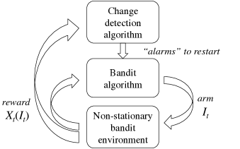
Our change-detection based framework consists of two components: a change detection algorithm and a bandit algorithm, as shown in Figure 1. At each time , the bandit algorithm outputs a decision based on its past observations of the bandit environment. The environment generates the corresponding reward of arm , which is observed by both the bandit algorithm and the change detection algorithm. The change detection algorithm monitors the distribution of each arm, and sends out a positive signal to restart the bandit algorithm once a breakpoint is detected. One can find that our framework is a generalization of the existing actively adaptive policies.
Since the bandit algorithms are well-studied in the bandit setting, what remains is to find a change detection algorithm, which works in the bandit environment. Change point detection problems have been well studied, see, e.g., the book (?). However, the change detection algorithms are applied in a context that is quite different from the bandit setting. There are two key challenges in adapting the existing change detection algorithms in the bandit setting.
(1) Unknown priors: In the context of the change detection problem, one usually assumes that the prior distributions before and after a change point are known. However, such information is unknown to the decision maker in the bandit setting. Even though there are some simple methods, such as estimating the priors and then applying the change detection algorithm like PHT, there are no analytical results in the literature.
(2) Insufficient samples: Due to the bandit feedback setting, the decision maker can only observe one arm at each time. However, there are change detection algorithms running in parallel since each arm is associated with a change detection procedure to monitor the possible mean shift. So the change detection algorithms in most arms are hungry for samples at each time. If the decision maker does not feed these change detection algorithms intentionally, the change detection algorithm may miss detection opportunities because they do not have enough recent samples.
4 Application of the Framework
In this section, we introduce our Change-Detection based UCB (CD-UCB) policy, which addresses the issue of insufficient samples. Then we develop a tailored CUSUM algorithm for the bandit setting to overcome the issue of unknown priors. Finally, we combine our CUSUM algorithm with the UCB algorithm as CUSUM-UCB policy, which is a specific instance of our change-detection based framework. Performance analysis is provided in Section 5.
4.1 CD-UCB policy
Suppose we have a change detection algorithm, CD, which takes arm index and observation as input at time , and it returns if there is an alarm for a breakpoint. Given such a change detection algorithm, we can employ it to control the UCB algorithm, which is our CD-UCB policy as shown in Algorithm 1. We clarify some useful notations as follows. Let be the last time that the CD alarms and restarts for arm before time . Then the number of valid observations (after the latest detection alarm) for arm up to time is denoted as . Let be the total number of valid observations for the decision maker. For each arm , let be the sample average and be the confidence padding term. In particular,
| (3) | ||||
| (4) |
where is some positive real number. Thus, the UCB index for each arm is . Parameter is a tuning parameter we introduce in the CD-UCB policy. At each time , the policy plays the arm
| (5) |
4.2 Tailored CUSUM algorithm
A change detection algorithm observes a sequence of independent random variables, , in an online manner, and outputs an alarm once a change point is detected. In the context of the traditional change detection problem, one assumes that the parameters and are known for the density function . In addition, is sampled from distribution under () before (after) the breakpoint. Let () be the mean of before (after) the change point. The CUSUM algorithm, originally proposed by (?), has been proven to be optimal in detecting abrupt changes in the sense of worst mean detection delay (?). The basic idea of the CUSUM algorithm is to take a function of the observed sample (e.g., the logarithm of likelihood ratio ) as the step of a random walk. This random walk is designed to have a positive mean drift after a change point and have a negative mean drift without a change. Hence, CUSUM signals a change if this random walk crosses some positive threshold .
We propose a tailored CUSUM algorithm that works in the bandit setting. To be specific, we use the first samples to calculate the average, Then we construct two random walks, which have negative mean drifts before the change point and have positive mean drifts after the change. In particular, we design a two-sided CUSUM algorithm, described in Algorithm 2, with an upper (lower) random walk monitoring the possible positive (negative) mean shift. Let () be the step of the upper (lower) random walk. Then and are defined as
| (6) |
Let () track the positive drift of upper (lower) random walk. In particular,
| (7) |
The change point is detected when either of them crosses the threshold . The parameter is important in the detection delay and false alarm trade-off. We discuss the choice of in Section 5.
4.3 CUSUM-UCB policy
Now we are ready to introduce our CUSUM-UCB policy, which is a CD-UCB policy with CUSUM as a change detection algorithm. In particular, it takes parallel CUSUM algorithms as CD in CD-UCB. Formal description of CUSUM-UCB can be found in Algorithm 3, provided in Section F in the supplementary material.
4.4 PHT-UCB policy
5 Performance Analysis
In this section, we analyze the performance in each part of the proposed algorithm: (a) our bandit algorithm (i.e., CD-UCB), and (b) our change detection algorithm (i.e., two-sided CUSUM). First, we present the regret upper bound result of CD-UCB for a given change detection guarantee. This is of independent interest in understanding the challenges of the non-stationary environment. Second, we provide performance guarantees of our modified CUSUM algorithm in terms of the mean detection delay, , and the expected number of false alarms up to time , . Then, we combine these two results to provide the regret upper bound of our CUSUM-UCB. The proofs are presented in our supplementary material.
Theorem 1.
(CD-UCB) Let . Under Assumption 1, for any and any arm , the CD-UCB policy achieves,
Recall that the regret of the CD-UCB policy is upper-bounded by . Therefore, given the parameter values (e.g., ) and the performance of a change detection algorithm (i.e., and ), we can obtain the regret upper bound of that change detection based bandit algorithm. By letting , we obtain the following result.
Corollary 1.
(CD-UCB) If and , then the regret of CD-UCB is
| (9) |
Remark 1.
If one can find an oracle algorithm that detects the change point with the properties that and , then one can achieve regret, which recovers the regret result in ? (?). We note that the WMD (Windowed Mean-shift Detection) change detection algorithm proposed by ? (?) achieves these properties when side observations are available.
In the next proposition, we introduce the result of Algorithm 2 about the conditional expected detection delay and the conditional expected number of false alarms given . Note that the expectations exclude the first slots for initial observations.
Proposition 1.
(CUSUM) Recall that is the tuning parameter in Algorithm 2. Under Assumptions 1 and 2, the conditional expected detection delay and the conditional expected number of false alarms satisfy
| (10) | ||||
| (11) |
where , is the non-zero root of and is the non-zero root of . In the case of , the algorithm restarts in at most time slots.
In the next theorem, we show the result for and when CUSUM is used to detect the abrupt change. Note again that the expectations exclude the first time slots.
Theorem 2.
Summing the result of Theorems 1 and 2, we obtain the regret upper bound of the CUSUM-UCB policy. To the best of our knowledge, this is the first regret bound for an actively adaptive UCB policy in the bandit feedback setting.
Theorem 3.
| Passively adaptive | Actively adaptive | |||||
|---|---|---|---|---|---|---|
| Policy | D-UCB | SW-UCB | Rexp3 | Adapt-EvE | CUSUM-UCB | lower bound |
| (?) | (?) | (?) | (?) | (?) | ||
| Regret | Unknown | |||||
Corollary 2.
Remark 2.
The choices of parameters depend on the knowledge of . This is common in the non-stationary bandit literature. For example, the discounting factor of D-UCB and sliding window size of SW-UCB depend on the knowledge of . The batch size of Rexp3 depends on the knowledge of , which denotes the total reward variation. It is practically viable when the reward change rate is regular such that one can accurately estimate based on history.
Remark 3.
As shown in ? (?), the lower bound of the problem is . Our policy approaches the optimal regret rate in an order sense.
Remark 4.
For the SW-UCB policy, the regret analysis result is (?). If is a constant with respect to , then term dominates and our policy achieves the same regret rate as SW-UCB. If goes to as increases, then the regret of CUSUM-UCB grows much slower than SW-UCB.
Table 1 summarizes the regret upper bounds of the existing and proposed algorithms in the non-stationary setting when is a constant in . Our policy has a smaller regret term with respect to compared to SW-UCB.
6 Simulation Results
We evaluate the existing and proposed policies in three non-stationary environments: two synthetic dataset (flipping and switching scenarios) and one real-world dataset from Yahoo! (?). Yahoo! dataset collected user click traces for news articles. Our PHT-UCB is similar to Adapt-EvE, but they are different in that Adapt-EvE ignores the issue of insufficient samples and includes other heuristic methods dealing with the detection points.
In the simulation, the parameters and are tuned around and based on the flipping environment. We suggest the practitioners to take the same approach because the choices of and in Corollary 2 are minimizing the regret upper bound rather than the regret. We use the same parameters and for CUSUM-UCB and PHT-UCB to compare the performances of CUSUM and PHT. Parameters are listed in Table 2 in Section G of the appendix. Note that and are obtained based on the prior knowledge of the datasets. The baseline algorithms are tuned similarly with the knowledge of and . We take the average regret over 1000 trials for the synthetic dataset.
6.1 Synthetic Datasets
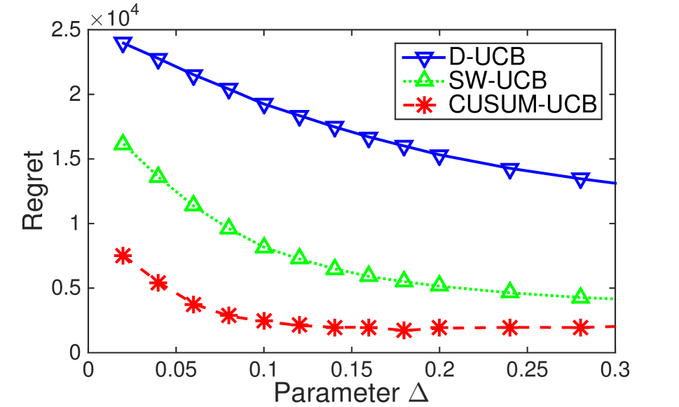
Flipping Environment. We consider two arms (i.e., ) in the flipping environment, where arm is stationary and the expected reward of arm flips between two values. All arms are associated with Bernoulli distributions. In particular, for any and
| (16) |
The two change points are at and . Note that is equivalent to . We let vary within the interval , and compare the regrets of D-UCB, SW-UCB and CUSUM-UCB to verify Remark 4. For this reason, results of other algorithms are omitted. As shown in Figure 2(a), CUSUM-UCB outperforms D-UCB and SW-UCB. In addition, the gap between CUSUM-UCB and SW-UCB increases as decreases.
Switching Environment. We consider the switching environment, introduced by ? (?), which is defined by a hazard function, , such that,
| (17) |
Note that denotes the uniform distribution over the interval and are independent samples from . In the experiments, we use the constant hazard function . All the arms are associated with a Bernoulli distribution.
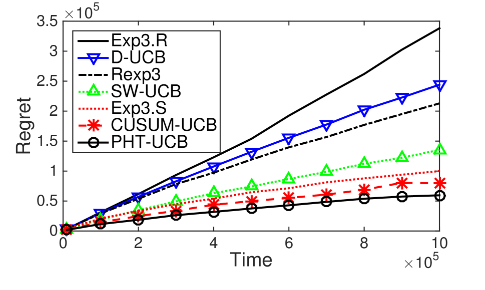
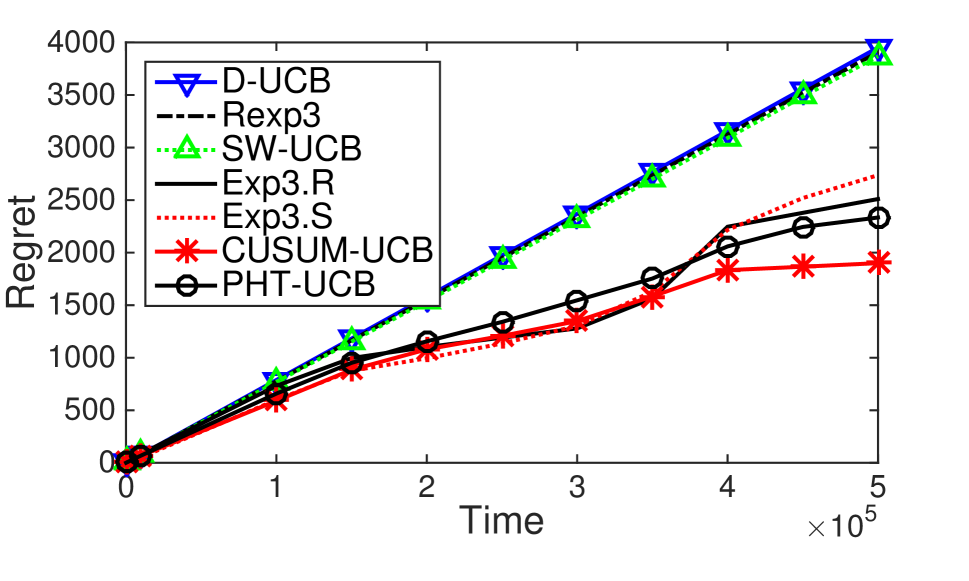
The regrets over the time horizon are shown in Figure 2(b). Although Assumptions 1 and 2 are violated, CUSUM-UCB and PHT-UCB outperform the other policies. To find the polynomial order of the regret, we use the non-linear least squares method to fit the curves to the model . The resulting exponents of Exp3.R, D-UCB, Rexp3, SW-UCB, Exp3.S, CUSUM-UCB and PHT-UCB are 0.92, 0.89, 0.85, 0.84, 0.83, 0.72 and 0.69, respectively. The regret of CUSUM-UCB and PHT-UCB shows the better sublinear function of time compared to the other policies. Another observation is that PHT-UCB performs better than CUSUM-UCB, although we could not find a regret upper bound for PHT-UCB. The reason behind is that the PHT test is more stable and reliable (due to the updated estimation ) in the switching environment.
6.2 Yahoo! Dataset
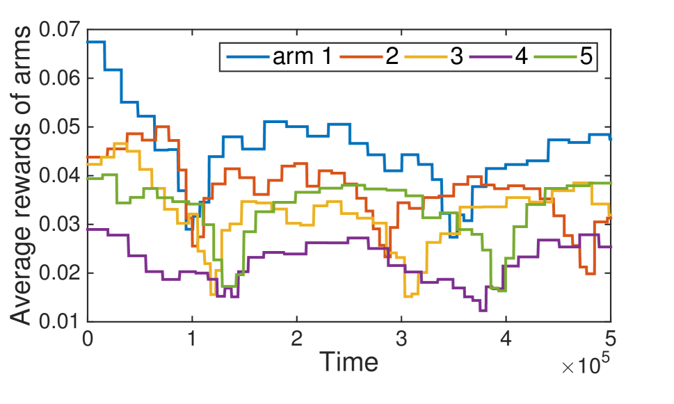
Yahoo! Experiment 1 (). Yahoo! has published a benchmark dataset for the evaluation of bandit algorithms (?). The dataset is the user click log for news articles displayed on the Yahoo! Front Page (?). Given the arrival of a user, the goal is to select an article to present to the user, in order to maximize the expected click-through rate, where the reward is a binary value for user click. For the purpose of our experiment, we randomly select the set of 5 articles (i.e., ) from a list of 100 permutations of possible articles which overlapped in time the most. To recover the ground truth of the expected click-through rates of the articles, we take the same approach as in ? (?), where the click-through rates were estimated from the dataset by taking the mean of an article’s click-through rate every 5000 time ticks (the length of a time tick is about one second), which is shown in Figure 3(a).
The regret curves are shown in Figure 3(b). We again fit the curves to the model . The resulting exponents of D-UCB, Rexp3, SW-UCB, Exp3.R, Exp3.S, CUSUM-UCB and PHT-UCB are 1, 1, 1, 0.81, 0.85, 0.69 and 0.79, respectively. The passively adaptive policies, D-UCB, SW-UCB and Rexp3, receive a linear regret for most of the time. CUSUM-UCB and PHT-UCB achieve much better performance and show sublinear regret, because of their active adaptation to changes. Another observation is that CUSUM-UCB outperforms PHT-UCB. The reason behind is that the Yahoo! dataset has more frequent breakpoints than the switching environment (i.e., high ). Thus, the estimation in PHT test may drift away before PHT detects the change, which in turn results in more detection misses and the higher regret.
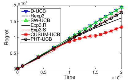
Yahoo! Experiment 2 (). We repeat the above experiment with . The regret curves are shown in Figure 4. We again fit the curves to the model . The resulting exponents of D-UCB, Rexp3, SW-UCB, Exp3.R, Exp3.S, CUSUM-UCB and PHT-UCB are 1, 1, 1, 0.88, 0.9, 0.85 and 0.9, respectively. The passively adaptive policies, D-UCB, SW-UCB and Rexp3, receive a linear regret for most of the time. CUSUM-UCB and PHT-UCB show robust performance in this larger scale experiment.
7 Conclusion
We propose a change-detection based framework for multi-armed bandit problems in the non-stationary setting. We study a class of change-detection based policies, CD-UCB, and provide a general regret upper bound given the performance of change detection algorithms. We then develop CUSUM-UCB and PHT-UCB, that actively react to the environment by detecting breakpoints. We analytically show that the regret of CUSUM-UCB is , which is lower than the regret bound of existing policies for the non-stationary setting. To the best of our knowledge, this is the first regret bound for actively adaptive UCB policies. Finally, we demonstrate that CUSUM-UCB outperforms existing policies via extensive experiments over arbitrary Bernoulli rewards and the real world dataset of webpage click-through rates.
Acknowledgment
This work has been supported in part by grants from the Army Research Office W911NF-14-1-0368 W911NF-15-1-0277, and MURI W911NF-12-1-0385, DTRA grant HDTRA1-14-1-0058, and NSF grant CNS-1719371.
References
- [2012] Agrawal, S., and Goyal, N. 2012. Analysis of thompson sampling for the multi-armed bandit problem. In COLT, 39.1–39.26.
- [2008] Alaya-Feki, A. B. H.; Moulines, E.; and LeCornec, A. 2008. Dynamic spectrum access with non-stationary multi-armed bandit. In 2008 IEEE 9th Workshop on Signal Processing Advances in Wireless Communications, 416–420. IEEE.
- [2015] Allesiardo, R., and Féraud, R. 2015. Exp3 with drift detection for the switching bandit problem. In Data Science and Advanced Analytics (DSAA), 2015. 36678 2015. IEEE International Conference on, 1–7. IEEE.
- [2002] Auer, P.; Cesa-Bianchi, N.; Freund, Y.; and Schapire, R. E. 2002. The nonstochastic multiarmed bandit problem. SIAM Journal on Computing 32(1):48–77.
- [2002] Auer, P.; Cesa-Bianchi, N.; and Fischer, P. 2002. Finite-time analysis of the multiarmed bandit problem. Machine learning 47(2-3):235–256.
- [1993] Basseville, M., and Nikiforov, I. V. 1993. Detection of abrupt changes: theory and application, volume 104. Prentice Hall Englewood Cliffs.
- [2014] Besbes, O.; Gur, Y.; and Zeevi, A. 2014. Stochastic multi-armed-bandit problem with non-stationary rewards. In Advances in neural information processing systems, 199–207.
- [2012] Bubeck, S., and Cesa-Bianchi, N. 2012. Regret analysis of stochastic and nonstochastic multi-armed bandit problems. arXiv preprint arXiv:1204.5721.
- [2017] Buccapatnam, S.; Liu, F.; Eryilmaz, A.; and Shroff, N. B. 2017. Reward maximization under uncertainty: Leveraging side-observations on networks. arXiv preprint arXiv:1704.07943.
- [2006] Cesa-Bianchi, N., and Lugosi, G. 2006. Prediction, learning, and games. Cambridge university press.
- [2012] Gallager, R. G. 2012. Discrete stochastic processes, volume 321. Springer Science & Business Media.
- [2008] Garivier, A., and Moulines, E. 2008. On upper-confidence bound policies for non-stationary bandit problems. arXiv preprint arXiv:0805.3415.
- [2007] Hartland, C.; Baskiotis, N.; Gelly, S.; Sebag, M.; and Teytaud, O. 2007. Change point detection and meta-bandits for online learning in dynamic environments. CAp 237–250.
- [1971] Hinkley, D. V. 1971. Inference about the change-point from cumulative sum tests. Biometrika 509–523.
- [2012] Kaufmann, E.; Korda, N.; and Munos, R. 2012. Thompson sampling: An asymptotically optimal finite-time analysis. In International Conference on Algorithmic Learning Theory, 199–213. Springer.
- [1981] Khan, R. A. 1981. A note on page’s two-sided cumulative sum procedure. Biometrika 717–719.
- [2006] Kocsis, L., and Szepesvári, C. 2006. Discounted ucb. In 2nd PASCAL Challenges Workshop, 784–791.
- [1985] Lai, T. L., and Robbins, H. 1985. Asymptotically efficient adaptive allocation rules. Advances in applied mathematics 6(1):4–22.
- [2011] Li, L.; Chu, W.; Langford, J.; and Wang, X. 2011. Unbiased offline evaluation of contextual-bandit-based news article recommendation algorithms. In Proceedings of the fourth ACM international conference on Web search and data mining, 297–306. ACM.
- [2016] Li, S.; Karatzoglou, A.; and Gentile, C. 2016. Collaborative filtering bandits. In Proceedings of the 39th International ACM SIGIR conference on Research and Development in Information Retrieval, 539–548. ACM.
- [1971] Lorden, G. 1971. Procedures for reacting to a change in distribution. The Annals of Mathematical Statistics 1897–1908.
- [2013] Mellor, J., and Shapiro, J. 2013. Thompson sampling in switching environments with bayesian online change detection. In Proceedings of the Sixteenth International Conference on Artificial Intelligence and Statistics, 442–450.
- [1954] Page, E. S. 1954. Continuous inspection schemes. Biometrika 41(1/2):100–115.
- [1984] Pollard, D. 1984. Convergence of Stochastic Processes. Springer.
- [2014] Srivastava, V.; Reverdy, P.; and Leonard, N. E. 2014. Surveillance in an abruptly changing world via multiarmed bandits. In Decision and Control (CDC), 2014 IEEE 53rd Annual Conference on, 692–697. IEEE.
- [1998] Sutton, R. S., and Barto, A. G. 1998. Reinforcement learning: An introduction, volume 1. MIT press Cambridge.
- [1933] Thompson, W. R. 1933. On the likelihood that one unknown probability exceeds another in view of the evidence of two samples. Biometrika 25(3/4):285–294.
- [2016] Wei, C.-Y.; Hong, Y.-T.; and Lu, C.-J. 2016. Tracking the best expert in non-stationary stochastic environments. In Advances In Neural Information Processing Systems, 3972–3980.
- [] Yahoo! Webscope program. http://webscope.sandbox.yahoo.com/catalog.php?datatype=r&did=49. [Online; accessed 18-Oct-2016].
- [2009] Yu, J. Y., and Mannor, S. 2009. Piecewise-stationary bandit problems with side observations. In Proceedings of the 26th Annual International Conference on Machine Learning, 1177–1184. ACM.
Appendix A Lemma List
We will make use of the following standard facts.
Lemma 1.
(Chernoff-Hoeffding bound) Let be random variables with common range and such that . Let . Then for all
| (18) | ||||
| (19) |
Lemma 1 states the well known Chernoff-Hoeffding inequalities, proof of which is referred to (?). The next two lemmas are used in the proof of Theorem 2.
Lemma 2.
(Wald’s identity) Let be independent and identically distributed, and let . Let be the interval of over which exists. For each , let . Let and be arbitrary, and let be the smallest for which either or . Then for each ,
| (20) |
Proof of Lemma 2 is referred to (?).
Lemma 3.
(Two-sided CUSUM) Let be independent random variables. For , define and . Let and . For , define and . Let . Then, we have that
| (21) |
Appendix B Proof of Theorem 1
Proof.
Recall that is the arm with the best UCB index at time , i.e., . In addition is the random arm sampled from uniform distribution. At each time , if the arm is played, then the CD-UCB algorithm is either sampling a random arm () or playing the arm with the best UCB index (). So, the probability that arm is chosen at time and arm is not the best arm is
| (22) |
By the definition of in equation (1), we have that
| (23) | ||||
| (24) | ||||
| (25) |
Now, it remains to bound the second term of (25), denoted by . Let be a constant defined as . Then we can decompose the event as
Consider an experiment of the CD-UCB over plays. Let be the number of false alarms up to time and be the detection delay of -th breakpoint on arm , where . Then, the total number of detection points, when the change detection algorithm CD signals an alarm on arm , is upper-bounded by . Let be the latest detection points (including false arms) up to time . For each arm , we define as the set of time slots that no breakpoint occurs after time slots away from the detection points.
| (26) |
Then, we can bound the term by
| (27) | ||||
For each , the event implies the following union of events
| (28) |
On the event , we have that
| (29) |
by the definition of . Thus, holds when . This implies that the last event of (28) is impossible. So we have that is at most
| (30) |
By the Lemma 1, we have that
| (31) | ||||
| (32) |
Let , be the length of intervals between successive detection points. Then, we have that . Let , we have that
| (33) | ||||
| (34) | ||||
| (35) |
Let be the expected number of false alarms in time horizon , and be the expected detection delay. Summing all the results, we have and
| (36) | ||||
Appendix C Proof of Proposition 1
Proof.
Let be a sequence of independent random variables with bounded support . Before (after) the change, the random variable follows a distribution with parameter (). Let () denote the mean before (after) the change. Under the Assumption 2, we have that . Note that we use the first samples to estimate the mean before the change by . Then, and become a non-trivial function of observation . We define the expected time excluding the first time slots until the alarm occurs as the average run length (ARL), which is consistent with the literature in change detection problems (?). In particular, let be the ARL function defined as
| (37) |
It is clear that Algorithm 2 is a symmetric version of two-sided CUSUM-type algorithm (?). Let and ( and ) be the upper (lower) side CUSUM random walk. Then, we define the ARL function for lower and upper side CUSUM as
| (38) | ||||
| (39) |
By Lemma 3, we have that
| (40) |
The ARL function characterizes the detection delay and false alarm performances of our CUSUM algorithm. In particular, is the mean detection delay, and is the mean time between false alarms. Thus, and . By (40), it remains to calculate and . In the following, we show the results for and obtain the results for by symmetry.
Let be a random walk. Let be the smallest such that crosses the bounded interval , i.e., . The procedure that monitors the stopping time that crosses the boundary is also called a sequential probability ratio test (SPRT). Then the lower side CUSUM can be viewed as a repeated SPRT such that CUSUM restarts the SPRT once crosses the boundary (i.e., ) and outputs an alarm the first time that crosses the boundary (i.e., ) (?). Let be the probability that SPRT ends up with . Let be the number of SPRT tests that CUSUM runs until an alarm. Then is a geometrically distributed random variable with parameter . Hence, we have that
| (41) | ||||
| (42) |
Let . Then, by Lemma 2 we have
| (43) |
We use the two implications from the Wald’s identity . For simplicity, we assume that when we consider the expectation of and . First, taking the derivative of both sides and letting , we have that
| (44) |
Second, letting such that and , we have that
| (45) |
By the Assumption 1, is the average of samples from distribution under . By Lemma 1, we have that
| (46) |
Now, we classify the possible scenarios into four different cases depending on and , under which we can derive the upper bound of the mean detection delay or the mean time between false alarms.
Case 1: and
Under , we show the upper bound of (mean detection delay of lower side CUSUM). Note that . Then, by (42) and (44) we have that
| (47) | ||||
| (48) | ||||
| (49) | ||||
| (50) |
Under , we show the lower bound of (mean time between false alarms of lower side CUSUM). Note that , which implies that . By (45), we have that
| (51) | ||||
| (52) | ||||
| (53) | ||||
| (54) |
Note that . Hence, we have that
| (55) |
Under , we obtain the lower bound of (mean time between false alarms of upper side CUSUM) with the similar arguments. In particular, , which implies that . Then we have that
| (56) |
Let . By (40), we have that
| (57) | ||||
| (58) |
Case 2: and
Similarly, we obtain the results for upper side CUSUM as
| (59) | ||||
| (60) |
Under , we check that . Hence, we have that
| (61) |
By (40), we have that
| (62) | ||||
| (63) |
Case 3:
When the estimate is large (), . Then we have that
| (64) |
Case 4:
When the estimate is small (), . Then we have that
| (65) |
∎
Appendix D Proof of Theorem 2
Note that the bounds for , and in the Proposition 1 are the conditional expectations under given . By the law of total expectation, we can obtain the expected bound results by taking expectation over . Let denote the expectation over . We classify the possible scenarios into two cases, under which we take the conditional expectations and sum the total expectation finally.
Case 1:
By the Proposition 1, given the condition and , we have that
| (66) | ||||
| (67) | ||||
| (68) |
First, we consider the upper bound of when . Let denote the probability density function (or probability mass function) of random variable . Then, we have that
| (69) | ||||
| (70) | ||||
| (71) |
We define . Note that is the minimum over a finite set of positive real numbers (i.e., ). Then, . Therefore, we have
| (72) | ||||
| (73) | ||||
| (74) | ||||
| (75) |
Hence, we have that
| (76) | ||||
| (77) |
The same result holds for . Note that by the Assumption 2. Then, we have that
| (78) |
Second, we consider the lower bound of and . By the Assumption 3, the is a Bernoulli random variable. Then, we have that
| (79) | ||||
| (80) |
Let () be the solution of . Then, the convexity of implies that . In addition, and satisfy
| (81) | ||||
| (82) |
Note that and always exist when . One can scale the reward linearly without changing the problem by function so that the expected reward is within the interval . Hence, we assume that and exist without loss of generality. We first derive a lower bound for (81).
| (83) | |||
| (84) | |||
| (85) | |||
| (86) | |||
| (87) | |||
| (88) | |||
| (89) |
Hence, we have that
| (90) | ||||
| (91) | ||||
| (92) |
Now, we derive a lower bound for (82). Similarly, we have that
| (93) | ||||
| (94) | ||||
| (95) | ||||
| (96) | ||||
| (97) |
Hence, by the Jensen’s inequality, we have that
| (98) | ||||
| (99) | ||||
| (100) | ||||
| (101) | ||||
| (102) | ||||
| (103) | ||||
| (104) |
Let and . Then, there exists a positive number , which depends on and , such that
| (105) | ||||
| (106) | ||||
| (107) | ||||
| (108) |
Similarly, we have that
| (109) |
Case 2:
By Assumption 3, the is the average of Bernoulli random variables. In other words, must be one of the points . Then there must be a gap between and . Let be the minimal gap of arm .333Note that denotes the floor function and denotes the ceiling function. We define the minimal gap of all arms as .
By the Proposition 1, the average run length is at most
| (110) |
Suppose that , then
| (111) | ||||
| (112) | ||||
| (113) | ||||
| (114) |
The same result holds when . Summing the results (78) (108) (109) (114), we derive the upper bound for the mean detection delay and the lower bound for number of false alarms within the horizon .
| (115) | ||||
| (116) | ||||
| (117) |
Note that the mean time between false alarm is . By the law of total expectation, we have that
| (118) |
By the Lemma 3 and (108) (109), we have that
| (119) |
Hence, we have that
| (120) | ||||
| (121) |
Appendix E Proof of Theorem 3
Appendix F CUSUM-UCB policy
CUSUM-UCB policy is a CD-UCB policy with CUSUM as a change detection algorithm. In particular, it takes parallel CUSUM algorithms as CD in CD-UCB. Since our CUSUM algorithm needs to estimate the mean first, we let the policy finish the estimation with observations as soon as possible. That is why we introduce the countdown timers in Algorithm 3. The performance of CUSUM-UCB depends on the parameters and . We discuss the joint choices of and in Sections 5 and 6.
Appendix G Simulation Parameters
| Environment | |||||||
|---|---|---|---|---|---|---|---|
| Flipping | |||||||
| Switching | |||||||
| Yahoo! 1 | |||||||
| Yahoo! 2 |
-
a
: We count breakpoints when the difference in mean rewards is greater than .