Momentum conservation and unitarity in parton showers and NLL resummation

Abstract

We present a systematic study of differences between NLL resummation and parton showers. We first construct a Markovian Monte-Carlo algorithm for resummation of additive observables in electron-positron annihilation. Approximations intrinsic to the pure NLL result are then removed, in order to obtain a traditional, momentum and probability conserving parton shower based on the coherent branching formalism. The impact of each approximation is studied, and an overall comparison is made between the parton shower and pure NLL resummation. Differences compared to modern parton-shower algorithms formulated in terms of color dipoles are analyzed.

I Introduction

Searches for new physics and measurements of Standard Model parameters at the Large Hadron Collider and possible future colliders require ever increasing precision in the analysis of multi-scale events. Large scale hierarchies in such reactions will generally result in large Bremsstrahlung effects. In order to reliably predict measurable quantities, such as a fiducial cross section, the radiative corrections determined in QCD perturbation theory must be resummed to all orders. Resummation was first performed for energy-energy correlations in $e^{+}e^{-}$ collisions Dokshitzer et al. (1980); Parisi and Petronzio (1979); Collins and Soper (1981), transverse momentum dependent cross sections in Drell-Yan events Sterman (1987); Catani and Trentadue (1989, 1991) and $e^{+}e^{-}$ hadronic event shapes Catani et al. (1993). Several observables in hadron collisions have also been resummed analytically Catani et al. (2000). Such calculations have been extended to very high precision and used, for example, to extract the strong coupling from experimental data in $e^{+}e^{-}$ annihilation to hadrons Dissertori et al. (2009); Gehrmann et al. (2010). Effective field theory methods Bauer et al. (2002a, b) also contribute to rapid progress in this field. General semi-analytic approaches to the problem have been constructed Kidonakis and Sterman (1997); Kidonakis et al. (1998a); Laenen et al. (1998); Bonciani et al. (2003); Banfi et al. (2002, 2005, 2015) and automated Gerwick et al. (2014) based on direct QCD resummation. They depend only on universal coefficients and are applicable to different processes and a large class of observables. An alternative to analytical calculations is the simulation of events in a Markov-Chain Monte-Carlo known as a parton showerFox and Wolfram (1980); Marchesini and Webber (1984); Sjöstrand (1985); Marchesini and Webber (1988). While the formal precision of this approach is comparable to analytic resummation only in processes with a trivial color structure at the leading order, parton-showers typically give a good description of experimental measurements and are therefore an integral part of the high-energy physics toolkit.

Even in the simplest scenarios the resummation performed by a parton shower is not identical to an analytic computation. This study will investigate the differences in some detail. We first show how a parton shower can be constructed that reproduces the pure next-to-leading logarithmic (NLL) resummed result as obtained by the semi-analytic C AESAR formalism Banfi et al. (2005). For simplicity we will focus on additive observables in $e^{+}e^{-}$ annihilation to jets. Starting from this algorithm, we successively include effects beyond NLL accuracy that arise from momentum and probability conservation, such that a traditional parton shower in the coherent branching formalism is recovered eventually. To our knowledge this is the first time that a systematic study of this type has been performed. While we focus on a very simple setup, for which parton showers have been shown to achieve NLL accuracy Catani et al. (1991), we argue that most differences investigated here will also arise in more complicated scenarios, such as hadron-hadron collisions and processes with a non-trivial color structure at the Born level. They will impact any prediction made for the Large Hadron Collider and possible future colliders, and – while formally sub-leading – they may be numerically large and should be taken into account as a systematic uncertainty.

This paper is organized as follows: Section II recalls those parts of the C AESAR formalism and of the parton shower formalism needed in this study. Section III presents the technical details of a modified parton shower reproducing exactly the analytic NLL result. Section IV analyzes the role of NLL approximations in detail by removing them from the previously constructed shower one-by-one. Section V compares the full parton-shower result against a more conventional parton-shower implementation, where soft double counting is removed by partial fractioning of the soft eikonal. Section VI presents our conclusions.

II NLL resummation and the parton shower formalism

We first review the methods used for analytic resummation in C AESAR Banfi et al. (2005) as well as the parton shower algorithm Fox and Wolfram (1980); Marchesini and Webber (1984); Sjöstrand (1985); Marchesini and Webber (1988). They are cast into a common language in order to allow an easy comparison between the two. We focus on the simplest case of resummation of a 2-jet observable in $e^{+}e^{-}\to\mathrm{jets}$, i.e. resummation of soft gluons emitted from a pair of two hard quark lines.

II.1 Prerequisites and notation

Following the C AESAR formalism, we denote the momenta of the hard partons as $p_{1},\ldots,p_{n}$. Additional soft emissions are denoted by $k$, and the observable we wish to compute by $v$. In general, the observable will be a function of both the hard and the soft momenta, $v=V(\{p\},\{k\})$, while in the soft approximation it reduces to a function of the soft momenta alone, $v=V(\{k\})$. In the rest frame of two hard legs, $i$ and $j$, considered to be the radiating color dipole, we can parametrize the momentum of a single emission as

$$k=z_{i,j}p_{i}+z_{j,i}p_{j}+k_{T,ij}\;,\qquad\text{where}\qquad k_{T,ij}^{2}=2p_{i}p_{j}\,z_{i,j}\,z_{j,i}\;.$$ (1)

We define the rapidity of the emission in this frame as $\eta_{ij}=1/2\ln(z_{i,j}/z_{j,i})$. The observable, computed as a function of $k$ when radiated collinear to the hard parton, $l$, can then be written as.

$$V(k)=\left(\frac{k_{T,l}}{Q}\right)^{a}e^{-b_{l}\eta_{l}}\;,$$ (2)

where, in the collinear limit, we have $k_{T,l}=k_{T,lj}$ and $\eta_{l}=\eta_{lj}$ for any $j\nparallel l$. We restrict our analysis to the case of additive observables, which can be calculated in the presence of multiple soft gluons as a simple sum, $V\left(k_{1},\dots,k_{n}\right)=\sum_{i}^{n}V(k_{i})$. Such observables are of great interest phenomenologically and, while relatively easy to compute, already exhibit most complications associated with the effects of NLL approximations.

The parton shower used in our study will be based on DGLAP evolution Gribov and Lipatov (1972); Lipatov (1975); Dokshitzer (1977); Altarelli and Parisi (1977). At NLL, for recursive infrared and collinear safe observables, gluon splitting only contributes at the inclusive level and is therefore taken into account effectively by working in the CMW scheme Catani et al. (1991). In analogy to the NLL C AESAR formalism, our parton shower will therefore only implement gluon radiation off the hard partons, and soft double counting will be removed by sectorization of the soft-emission phase space. Technical details are given in Sec. III, and a comparison to more conventional parton showers, which include gluon splitting, is performed in Sec. V. The basis for DGLAP evolution are the collinear factorization properties of QCD matrix elements. With $|\mathcal{M}_{n}(1,\ldots,n)|^{2}$ being the squared $n$-parton matrix element, the factorization formula in the limit that partons $i$ and $j$ become collinear reads

$$\mathop{d\Phi_{n+1}}\left|\mathcal{M}_{n+1}(1,..,i,..,j,..,n)\right|^{2}\approx\mathop{d\Phi_{n}}\left|\mathcal{M}_{n}(1,..,ij,..,n)\right|^{2}\;\frac{\mathop{dt}}{t}\mathop{dz}\frac{\mathop{d\phi}}{2\pi}\,\frac{\alpha_{s}}{2\pi}P_{ij\,i}(z)\;.$$ (3)

In this context, $\mathop{d\Phi_{n}}$ is the $n$-particle phase space element, and $P_{ij\,i}(z)$ is the Altarelli-Parisi splitting kernel associated with the branching of an intermediate parton $ij$ into partons $i$ and $j$. Except for the analysis in Sec. V, the only relevant splitting kernel in our study is the quark-to-quark transition

$$P_{qq}\left(z\right)=C_{F}\left[\frac{2}{1-z}-\left(1+z\right)\right]~{}.$$ (4)

The treatment of gluon radiators is discussed in App. A. We denote the unregularized splitting probability between two scales, $t$ and $t^{\prime}$, as

$$R(t^{\prime},t)=\int_{t^{\prime}}^{t}\frac{\mathop{d\bar{t}}}{\bar{t}}\;R^{\prime}(\bar{t})\;\qquad\text{where}\qquad R^{\prime}(t)=\int_{z_{\rm min}(t)}^{z_{\rm max}(t)}dz\;\frac{\alpha_{s}}{2\pi}P_{qq}(z)\;.$$ (5)

Following standard practice to improve the logarithmic accuracy of the resummation, the strong coupling is evaluated at the transverse momentum of the gluon Amati et al. (1980), and the soft enhanced term of the splitting functions is rescaled by $1+\alpha_{s}/(2\pi)K$, where $K=(67/18-\pi^{2}/6)\,C_{A}-10/9\,T_{R}\,n_{f}$ Catani et al. (1991). The latter method is known as the CMW scheme.

The integration boundaries for $z$ depend on the evolution variable and are given by the constraint that the momentum in the anti-collinear direction must be preserved. For the case of evolution in collinear transverse momentum, $k_{T}^{2}=2p_{i}p_{j}\,z(1-z)$, we obtain $z_{\rm min/max}=(1\mp\sqrt{1-4k_{T}^{2}/Q^{2}})/2$ (cf. Sec. IV). The probability for no splitting between two scales can be inferred from a unitarity constraint, i.e. the condition that the parton shower be probability conserving. For final-state evolution the no-branching probability is given by

$$\Pi(t^{\prime},t)=e^{-R(t,t^{\prime})}\;.$$ (6)

Note that this particular form of the no-branching probability is equivalent to the Sudakov form factor only at leading order, cf. App. A. Since we neglect gluon splitting, the functional form of $R$ is unchanged until the shower terminates, which greatly simplifies the calculation. The parton shower algorithm solves for the scale $t^{\prime}$, based on a starting scale $t$ and the total branching probability (differential in $\ln t$),

$$\mathcal{P}(t^{\prime},t)=\frac{d\,\Pi(t^{\prime},t)}{d\ln t^{\prime}}\;.$$ (7)

It terminates when a cutoff scale $t_{c}$ is reached. Typically, $t_{c}$ is defined such as to mark the transition to the non-perturbative regime, i.e. the region where $\alpha_{s}/(2\pi)\approx 1$.

II.2 Casting analytic resummation into the parton shower language

To enable a comparison with the semi-analytic resummation framework of C AESAR , we consider the cumulative cross section in an arbitrary observable, $v$, defined as

$$\Sigma\left(v\right):=\frac{1}{\sigma}\int^{v}\mathop{d\bar{v}}\frac{\mathop{d\sigma}}{\mathop{d\bar{v}}}\;.$$ (8)

The calculation is simplified by choosing a parton shower evolution variable, $\xi$, that (up to a power) corresponds to $V(k)$

$$\xi=k_{T}^{2}\,(1-z)^{-\frac{2b}{a+b}}\;.$$ (9)

This implies that splittings giving the largest contribution to the observable are produced first. Note that here and in the following we use $k_{T}=k_{T,l}$ and $\eta=\eta_{l}$.

If the effects of multiple emissions could be ignored, the cumulative cross section in Eq. (8) would be given by the square of the survival probability, Eq. (6), corresponding to the fact that radiation of a single gluon can originate from either of the two hard legs in the two-quark leading-order final state. It would then be sufficient to compute the probability $R(v)=R(v,1)$ for emissions resulting in observable values larger than $v$. Already at the level of a single emission this would lead to double counting Marchesini and Webber (1984). The problem can be circumvented by sectorizing the phase space using the requirement $\eta>0$. Note that this constraint is not strictly necessary for the collinear part of the splitting function if the parton shower implementation is capable of handling negative weights. However, this is not the case for most traditional shower algorithms, which prompts us to apply the condition to the entire splitting function. The combined probability for a single emission from any of the two hard legs at $\xi>Q^{2}v^{2/(a+b)}$ can then be written as

$$R_{\rm PS}(v)=2\int_{Q^{2}v^{\frac{2}{a+b}}}^{Q^{2}}\frac{\mathop{d\xi}}{\xi}\;\int_{z_{\rm min}}^{z_{\rm max}}dz\;\frac{\alpha_{s}\big{(}\xi(1-z)^{\frac{2b}{a+b}}\big{)}}{2\pi}\,C_{F}\left[\frac{2}{1-z}-(1+z)\right]\,\Theta\bigg{(}\!\ln\frac{(1-z)^{\frac{2a}{a+b}}}{\xi/Q^{2}}\bigg{)}\;.$$ (10)

This should be compared to Eq. (2.17) of Ref. Banfi et al. (2005), which can be rewritten in our parametrization as

$$R_{\rm NLL}(v)=2\int_{Q^{2}v^{\frac{2}{a+b}}}^{Q^{2}}\frac{\mathop{d\xi}}{\xi}\;\left[\,\int_{0}^{1}dz\;\frac{\alpha_{s}\big{(}\xi(1-z)^{\frac{2b}{a+b}}\big{)}}{2\pi}\frac{2\,C_{F}}{1-z}\Theta\bigg{(}\!\ln\frac{(1-z)^{\frac{2a}{a+b}}}{\xi/Q^{2}}\bigg{)}-\frac{\alpha_{s}(\xi)}{\pi}\,C_{F}B_{q}\right]\;.$$ (11)

A brief summary of semi-analytic resummation based on Banfi et al. (2005) and using Eq. (11) can be found in App. B. The no-emission probability based on $R_{\rm NLL}(v)$ can also be computed in a Markovian Monte-Carlo simulation, by starting from the parton-shower expression, Eq. (10), and performing the following manipulations:

• The $z$-integration in the soft term runs from 0 to $1-(\xi/Q^{2})^{(a+b)/2a}$, where the upper bound stems from the requirement that $\eta>0$ (the $\Theta$-function in Eq. (10)), eliminating the double counting of soft-gluon radiation.

• The collinear term proportional to $(1+z)$ is integrated from 0 to 1 in order to produce the collinear anomalous dimension, $B_{q}$. At the same time, $\alpha_{s}$ is evaluated at $\xi$.

Note in particular that the $z$-integration is extended beyond the values $z_{\rm min}$ (and $z_{\rm max}$ in the collinear case) allowed by local four-momentum conservation. This will be one of the effects investigated in Sec. IV.

The complete parton-shower prediction of the cumulative cross section, $\Sigma(v)$, including effects from arbitrarily many emissions, and using the approximation $V(\{p\},\{k\})=\sum_{i}V(k_{i})$ is given by

$$\Sigma_{\mathrm{PS}}\left(v\right) =\sum_{m=0}^{\infty}\left(\prod_{i=1}^{m}\int_{\xi_{c}}^{\xi_{i-1}}\frac{\mathop{d\xi_{i}}}{\xi_{i}}\,R_{\rm PS}^{\prime}(\xi_{i})\,e^{-R_{\rm PS}(\xi_{i-1},\xi_{i})}\right)e^{-R_{\rm PS}(\xi_{m},\xi_{c})}\;\Theta\bigg{(}v-\sum_{j=1}^{m}V(t_{j})\bigg{)}\bigg{|}_{\xi_{0}=Q^{2}}$$ (12)

$$=e^{-R_{\rm PS}(Q^{2},t_{c})}\sum_{m=0}^{\infty}\frac{1}{m!}\left(\prod_{i=1}^{m}\int_{t_{c}}^{Q^{2}}\frac{\mathop{dt_{i}}}{t_{i}}\,R_{\rm PS}^{\prime}(t_{i})\right)\Theta\bigg{(}v-\sum_{j=1}^{m}V(t_{j})\bigg{)}\;.$$

We compare Eq. (12) to the main result of Banfi et al. (2002), which reads

$$\Sigma_{\mathrm{NLL}}\left(v\right)=e^{-R_{\rm NLL}(v)}\mathcal{F}\left(v\right)\;.$$ (13)

The exponential corresponds to the pure survival probability in terms of Eq. (11). The function $\mathcal{F}\left(v\right)$ accounts for the effect of multiple emissions. For the simple observables considered here it can be written as Banfi et al. (2005):

$$\mathcal{F}\left(v\right)=\lim_{\epsilon\to 0}\mathcal{F}_{\epsilon}\left(v\right)\;,\qquad\text{where}\qquad\mathcal{F}_{\epsilon}\left(v\right)=e^{R_{\rm NLL}^{\prime}(v)\ln\epsilon}\sum_{m=0}^{\infty}\frac{1}{m!}\left(\prod_{i=1}^{m}R_{\rm NLL}^{\prime}(v)\int_{\epsilon}^{1}\frac{\mathop{d\zeta_{i}}}{\zeta_{i}}\right)\Theta\bigg{(}1-\sum_{j=1}^{m}\zeta_{j}\bigg{)}\;.$$ (14)

Following the notation of Ref. Banfi et al. (2005), $R_{\rm NLL}^{\prime}(v)$ is the derivative of $R$ with respect to $L=-\ln v$, excluding all terms formally not relevant at NLL accuracy. Note that Eq. (14) is a pure NLL contribution to $\Sigma_{\rm NLL}(v)$, as $R^{\prime}(v)$ by itself is sub-leading. If we intend to generate Eq. (14) using a parton shower, the branching probability, Eq. (10), must be modified such as to reflect the differentiation w.r.t. the lower integration limit in Eq. (11), which leads to $\xi=Q^{2}v^{2/(a+b)}$, as well as the condition that higher logarithmic terms are dropped in $R^{\prime}(v)$. We can satisfy these constraints using the following modifications of the plain parton shower:

• The $z$-integration in the soft term runs from 0 to $1-v^{1/a}$.

• The strong coupling runs at one loop and is evaluated at $v^{2/(a+b)}(1-z)^{2b/(a+b)}$.

• The collinear term is dropped.

We can now rewrite Eq. (13) in a form that is similar to Eq. (12)

$$\Sigma\left(v\right)=\exp\left\{-\int_{v}\frac{\mathop{d\xi}}{\xi}R^{\prime}_{>v}(\xi)-\int_{v_{\mathrm{min}}}^{v}\frac{\mathop{d\xi}}{\xi}R^{\prime}_{<v}(\xi)\right\}\times\sum_{m=0}^{\infty}\frac{1}{m!}\left(\prod_{i=1}^{m}\int_{v_{\mathrm{min}}}\frac{\mathop{d\xi_{i}}}{\xi_{i}}R^{\prime}_{<v}(\xi_{i})\right)\Theta\bigg{(}v-\sum_{j=1}^{m}V(\xi_{j})\bigg{)}\;.$$ (15)

with $R^{\prime}$ given by

$$R^{\prime}_{\lessgtr v}(\xi)=\frac{\alpha_{s}^{\lessgtr v,\mathrm{soft}}\big{(}\mu^{2}_{\lessgtr}\big{)}}{\pi}\int_{z^{\rm min}}^{z^{\mathrm{max}}_{\lessgtr v,\mathrm{soft}}}\mathop{dz}\frac{C_{\mathrm{F}}}{1-z}-\frac{\alpha_{s}^{\lessgtr v,\mathrm{coll}}\big{(}\mu^{2}_{\lessgtr v}\big{)}}{\pi}\int_{z^{\rm min}}^{z^{\mathrm{max}}_{\lessgtr v,\mathrm{coll}}}\mathop{dz}C_{\mathrm{F}}\frac{1+z}{2}\;.$$ (16)

	Resummation	Parton Shower	Figure			Resummation	Parton Shower	Figure
$z^{\mathrm{max}}_{>v,\mathrm{soft}}$	$1-(\xi/Q^{2})^{\frac{a+b}{2a}}$		n.a.		$z^{\mathrm{max}}_{>v,\mathrm{coll}}$	$1$	$1-(\xi/Q^{2})^{\frac{a+b}{2a}}$	2
$\mu^{2}_{>v,\mathrm{soft}}$	$\xi(1-z)^{\frac{2b}{a+b}}$		n.a.		$\mu^{2}_{>v,\mathrm{coll}}$	$\xi$	$\xi(1-z)^{\frac{2b}{a+b}}$	2
$\alpha_{s}^{>v,\mathrm{soft}}$	2-loop CMW		n.a.		$\alpha_{s}^{>v,\mathrm{coll}}$	1-loop	2-loop CMW	5
$z^{\mathrm{max}}_{<v,\mathrm{soft}}$	$1-v^{\frac{1}{a}}$	$1-(\xi/Q^{2})^{\frac{a+b}{2a}}$	3		$z^{\mathrm{max}}_{<v,\mathrm{coll}}$	$0$	$1-(\xi/Q^{2})^{\frac{a+b}{2a}}$	6
$\mu^{2}_{<v,\mathrm{soft}}$	$Q^{2}v^{\frac{2}{a+b}}(1-z)^{\frac{2b}{a+b}}$	$\xi(1-z)^{\frac{2b}{a+b}}$	3		$\mu^{2}_{<v,\mathrm{coll}}$	n.a.	$\xi(1-z)^{\frac{2b}{a+b}}$	6
$\alpha_{s}^{<v,\mathrm{soft}}$	1-loop	2-loop CMW	5		$\alpha_{s}^{<v,\mathrm{coll}}$	n.a.	2-loop CMW	6

Table 1: Choices of parameters in Eq. (15) leading to Eq. (13) (NLL resummation) and Eq. (12) (parton shower). The effects of switching between the two parametrizations are investigated in the figure referred to in the last column. More details can be found in Sec. IV.

The choices of $\alpha_{s}$, $z^{\rm max}$ and $\mu^{2}$ corresponding to NLL resummation in the C AESAR formalism and in a DGLAP-based parton shower are given in Tab. 1. The physical limits on the $z$-integral in Eq. (10), which are a consequence of local four-momentum conservation, are not easily formulated in terms of $\xi$ and will be investigated separately in Sec. IV. It is interesting to note that $\mathcal{F}\left(v\right)$ by itself can be extracted from the same formalism by starting the shower evolution at $Q^{2}v^{\frac{2}{a+b}}$. This fact has been used in the past to construct a dipole shower for the resummation of non-global logarithms Dasgupta and Salam (2001).

III Markov-Chain Monte Carlo implementation

As described in Sec. II, the NLL resummation is nearly equivalent to a parton shower at the single-emission level. The differences lie in the treatment of the collinear term and of the lower integration boundary on $z$. These differences also introduce a change in the scale of the running coupling in Eq. (15). The choice of integration boundaries in the analytic resummation implies that the splitting function turns negative in parts of the phase space. To deal with this situation in the Monte Carlo simulation, we use the methods discussed in Höche et al. (2010); Lönnblad (2013). Splittings are generated according to an overestimate of the strong coupling and the splitting kernel

$$\alpha_{s}^{\rm max}P_{\mathrm{max}}\left(z\right)=\alpha_{s}^{\rm max}C_{\mathrm{F}}\left[\frac{2}{1-z}\Theta\left(z_{\mathrm{max}}^{\prime}-z\right)+\gamma\Theta\left(z-z_{\mathrm{max}}^{\prime}\right)\right]$$ (17)

with an in principle arbitrary constant $\gamma$. For practical calculations we choose $\gamma=2$. Note that the values of $z^{\mathrm{max}}_{\mathrm{soft}}$ and $z_{\mathrm{coll}}^{\mathrm{max}}$ are overestimated by a common value in $P_{\mathrm{max}}$, which we have made explicit by writing $z_{\rm max}^{\prime}$. Splittings are vetoed with a constant probability $1/C$ and are associated with a weight

$$\omega=\frac{C\;\alpha_{s}^{\rm res}P_{\mathrm{res}}\left(z\right)}{\alpha_{s}^{\rm max}P_{\mathrm{max}}\left(z\right)}\times\left\{\begin{array}[]{cc}\displaystyle 1&\text{if accepted}\\[5.69054pt] \displaystyle\frac{\alpha_{s}^{\rm max}P_{\mathrm{max}}\left(z\right)-\alpha_{s}^{\rm res}P_{\mathrm{res}}\left(z\right)}{\left(C-1\right)\alpha_{s}^{\rm res}P_{\mathrm{res}}\left(z\right)}&\text{if rejected}\end{array}\right.$$ (18)

This correction accounts in particular for the negative sign of the integrand, Eq. (19), in the region $z>z_{\rm max}^{\rm soft}$. In addition, it is possible to veto emissions violating the condition $\sum_{i}V(k_{i})<v$, which would contribute with zero weight, to improve numerical accuracy Lönnblad (2013). The value of $C$ determines how many emissions are proposed, and thus potentially vetoed. It can again in principle be an arbitrary constant larger than $1$, but is relevant for the speed of convergence. We choose $C=2$ in our implementation.
The kernel eventually used for NLL resummation is given by

$$\alpha_{s}^{\rm res}P_{\mathrm{res}}=C_{\mathrm{F}}\left[\alpha_{s}(\mu^{2}_{\rm soft})\frac{2}{1-z}\Theta\left(z^{\mathrm{max}}_{\rm soft}-z\right)-\alpha_{s}(\mu^{2}_{\rm coll})(1+z)\Theta\left(z^{\mathrm{max}}_{\rm coll}-z\right)\right]\;,$$ (19)

with $z_{\mathrm{max}}$ and $\mu^{2}$ chosen according to Table 1.

For multiple emissions $P_{\rm res}$ explicitly depends on $v$. We therefore first choose a value for $v$ and then run the parton shower, implementing the $z$ integration bounds and the scale of the strong coupling as defined in Tab. 1. This is a highly inefficient procedure to compute the cumulative cross section. If probability was conserved, the same distribution could be obtained by running the parton shower, computing $v$, filling the histogram in each bin with lower edge larger than $v$, and filling the histogram in the bin containing $v$ with weight $(v_{\rm max}-v)/\Delta v$, where $v_{\rm max}$ is the upper bin edge and $\Delta v$ is the bin width. This will be the method used to compute the predictions in Fig. 6 and Sec. V. While at the level of accuracy we are interested in, it is sufficient to set the cutoff scale of the parton shower to some numerically small value in $\xi$, exact agreement with the analytic calculation is expected only if the calculation is performed for a finite $\epsilon$, and the parton-shower cutoff is set to $\xi_{c}=\epsilon v$. We can verify that in this situation we reproduce the analytic result for finite $\epsilon$ in Eq. (14) and investigate the convergence towards the analytic result for $\epsilon\to 0$. Figure 1 presents the corresponding comparison for different values of $\epsilon$ in the case of the thrust 1(a) Farhi (1977), a BKS observable 1(b) Berger et al. (2003a, b) and a fractional energy correlation 1(c) Banfi et al. (2005). The definitions of the observables and related resummation coefficients are listed in App. C.

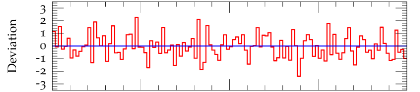
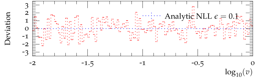
(a)  Thrust

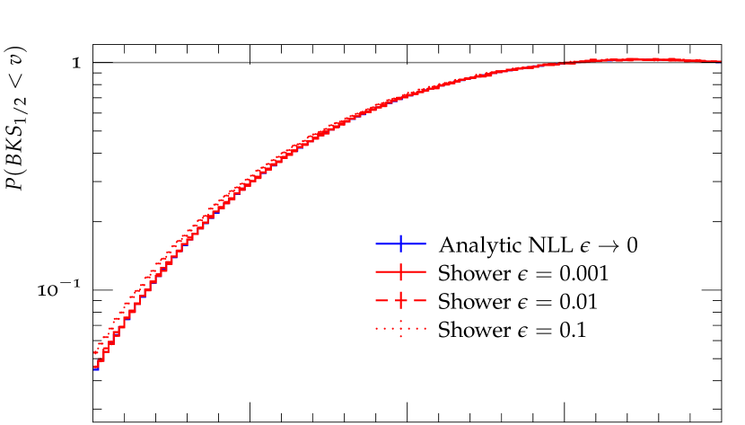
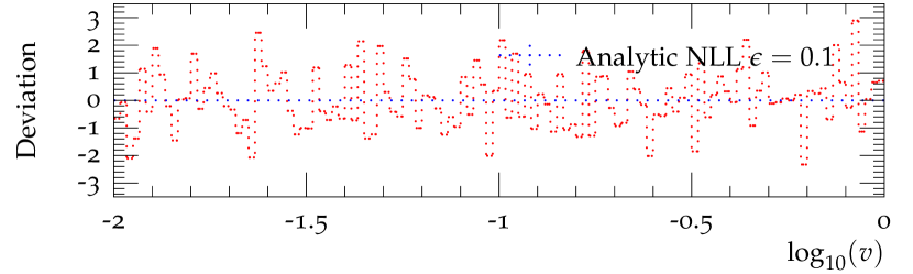
(b)  BKS_1/2

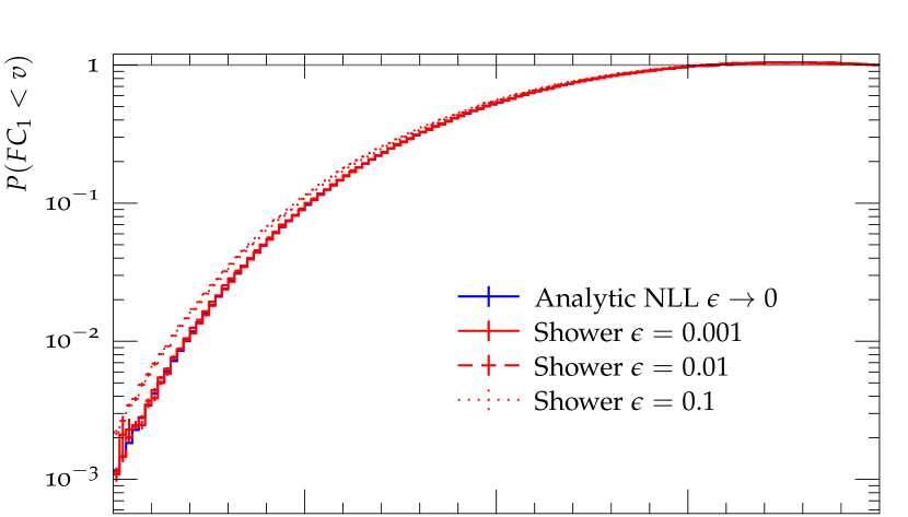
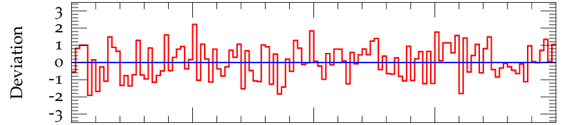
(c)  FC₁

Figure 1: Thrust variable $1-T$ 1(a), BKS observable with $x=1/2$ 1(b) and fractional energy correlation with $x=1$ 1(c) for different values of the cutoff $\epsilon$ in Eq. (14). The respective analytic results for $\mathcal{F}_{\epsilon}(v)$ are used as a reference in the ratio plots.

IV Effects of approximations

This section is dedicated to the detailed investigation of the effects of local four-momentum conservation and approximations made in the NLL calculation compared to the parton shower. In order to cover different choices of the parameters $a$ and $b$, we again present results for the thrust, a BKS observable ($x=1/2$) and a fractional energy correlation ($x=1$). All distributions are shown for $Q=91.2~{}\mathrm{GeV}$, and for a strong coupling defined by $\alpha_{s}(Q^{2})=0.118$ and a fixed number of flavors, $n_{f}=5$. We have cross-checked all of our predictions using two independent Monte-Carlo implementations based on Höche (2015).

We first investigate constraints arising from momentum conservation in the anti-collinear direction at single emission level, which reads

$$Q^{2}>2p_{i}p_{j}=\frac{k_{T}^{2}}{z(1-z)}\;.$$ (20)

This induces both a lower and an upper bound on $z$ given by $z_{\rm min/max}=(1\mp\sqrt{1-4k_{T}^{2}/Q^{2}})/2$. Figure 2 shows a comparison between the pure NLL predictions and those where this constraint has been implemented. The effect on the cumulative distributions is moderate, about 5% in the medium and low-$v$ region. In addition, we investigate the effect of choosing the scale in the collinear term to be $k_{T}^{2}$. This alters the slope of the thrust and BKS_1/2 distributions in the small-$v$ region, due to additional sub-leading logarithmic terms in $R(v)$.

The upper bound $z_{\rm max}$ is generally weaker than the constraint arising from the condition $\eta>0$, listed in Tab. 1. Figure 2 displays the additional effect on the NLL prediction when this constraint is applied in form of $z_{\lessgtr v,\rm coll}^{\rm max}$ as used in typical parton showers (cf. Eq. (10)). The effects are about 10% on all observables, and they lower the prediction for $\Sigma(v)$ due to an increased branching probability. Again, we also investigate the effect of choosing the scale in the collinear term to be $k_{T}^{2}$, which generates the same slope differences at small $v$ observed before.

(a)  Thrust

(b)  BKS_1/2

(c)  FC₁

Figure 2: Effects arising from momentum-conservation in the anti-collinear direction and from phase-space sectorization (removal of soft double counting in typical parton-shower implementations). Both are effects at the single-emission level, impacting terms in $R(v)$, cf. Tab. 1.

Next we investigate the effect of lifting the restriction on the $z$ integration in the calculation of $\mathcal{F}(v)$, i.e. removing the constraint $z<1-v^{1/a}$ if $\xi<Q^{2}v^{2/(a+b)}$ and replacing it by the constraint $\eta>0$. In this case $R^{\prime}(v)$ must be computed down to very small scales in Eq. (14), (except for FC₁) and it becomes mandatory to introduce an additional cutoff, as one would otherwise need to evaluate $\alpha_{s}$ at values where perturbation theory is no longer valid. We choose to implement this by adding the requirement $k_{T}^{\rm min}=0.5~{}{\rm GeV}$. The difference to the pure NLL result is shown in Fig. 3. Independent of the observable, this change is one of the largest differences observed in this study. The large relative difference between the pure NLL result and the modified prediction at small $v$ shows that sub-leading logarithmic effects become important.

(a)  Thrust

(b)  BKS_1/2

(c)  FC₁

Figure 3: Effect of replacing the constraint $z<1-v^{1/a}$ for $\xi<Q^{2}v^{2/(a+b)}$ by the phase-space sectorization constraint, $\eta>0$ and effects arising from the evaluation of the strong coupling at $k_{T}^{2}$ with $k_{T}^{\rm min}=0.5~{}{\rm GeV}$.

We also study the effect originating in the evaluation of the running coupling at $Q^{2}v^{2/(a+b)}(1-z)^{2b/(a+b)}$ if $\xi<Q^{2}v^{2/(a+b)}$. Again we implement the constraint $k_{T}^{\rm min}=0.5~{}{\rm GeV}$. Figure 3 shows that the predictions for all observables exhibit relatively large changes. They also show convergence issues at small values, which arise from the lower cutoff in $k_{T}$, leading to an insufficient sampling of $\mathcal{F}$ at higher number of emissions. This effect is most pronounced in FC₁, where it starts to appear around $10^{-1.5}$. Note, however, that practical measurements of FC₁ would be impacted by non-perturbative corrections in this regime. The problem is therefore purely academic in nature, hence we do not attempt to solve it here.

Formally the CMW scheme is the key to achieving NLL accuracy in a parton-shower computation of the observables considered here Catani et al. (1991). The numerical impact on $R(v)$ is investigated in Fig. 4.

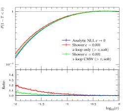
(a)  Thrust

(b)  BKS_1/2

(c)  FC₁

Figure 4: Effects of replacing 2-loop CMW running of $\alpha_{s}$ in the leading terms of the NLL result. The red line is computed without the CMW scheme, while the green line is computed by using the CMW scheme at 1-loop.

Figure 5 displays the effect of replacing 1-loop by 2-loop running couplings and of using the CMW scheme in sub-leading terms of the NLL calculation (cf. Tab. 1). The red line is computed by making the replacements only in the soft-enhanced part of the splitting function for $\xi<Q^{2}v^{2/(a+b)}$, and the red dotted line corresponds to not using the CMW scheme if $\xi<Q^{2}v^{2/(a+b)}$. It is evident that the effects are sizable over most of the observable range, and most pronounced at small $v$. The use of the CMW scheme has the biggest impact. Note in particular that not using the CMW scheme in the computation of $\mathcal{F}(v)$ has nearly the same impact as not using the CMW scheme in the computation of $R(v)$.

(a)  Thrust

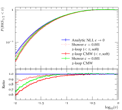
(b)  BKS_1/2

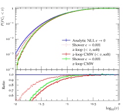
(c)  FC₁

Figure 5: Effects of replacing 1-loop by 2-loop CMW running of $\alpha_{s}$ in the sub-leading terms of the NLL result. The red line is computed by making the replacements only in the soft-enhanced term if $\xi<Q^{2}v^{2/(a+b)}$, the red dotted line corresponds to not using the CMW scheme in this region.

Figure 6 shows the cumulative effect of all changes discussed so far. In addition we present results from a simulation where the observable is computed using its definition in terms of four-momenta rather than using the soft approximation in Eq. (2) (see App. C for details). In this context it becomes important to take into account that emissions away from the strict soft limit inevitably change the momenta of the hard partons. Subsequent emissions are then computed based on the momenta of the quark lines with recoil effects taken into account. This can have a significant impact on the result, depending on the precise definition of the transverse momentum and momentum fraction. The magenta line in Fig. 6 corresponds to the conventions of Catani and Seymour (1997), while the green line corresponds to the conventions of Höche and Prestel (2015). In the latter case the transverse momentum coincides with Eq. (2.5) of Banfi et al. (2005). Note that the phase-space sectorization constraint, $\eta>0$, generates a different restriction on $z$ once recoil is taken into account, and that this condition depends on the choice of evolution and splitting variable.

(a)  Thrust

(b)  BKS_1/2

(c)  FC₁

Figure 6: Comparison of pure NLL resummation and plain DGLAP parton shower, effects of approximating the observable compared to exact calculation using four-momenta and evolution in dipole-$k_{T}$.

V Comparison with a dipole-like parton shower

This section presents a comparison of our previous results with predictions from a dipole-like parton shower. In such parton showers the soft enhanced part of the collinear splitting function is typically replaced by a partial fraction of the soft eikonal matched to the collinear limit Ellis et al. (1981); Catani and Seymour (1997). At the same time, the phase-space sectorization is removed, i.e. the restriction $\eta>0$ is lifted. A complete description of the parton-shower algorithm employed here can be found in Höche and Prestel (2015).

Figure 7 shows a comparison between results from the dipole-like parton shower in its default configuration (including gluon splitting) and from a modified version, tailored to match the settings of the parton shower used in Sec. IV, Fig. 6. It is interesting to observe that the dipole-shower prediction lies between the parton-shower result and the analytic result for all observables, and in the case of thrust agrees very well with the analytic prediction. In the measurable range at LEP energies, the predictions for FC₁ also agree fairly well between the dipole-shower and the analytic result.

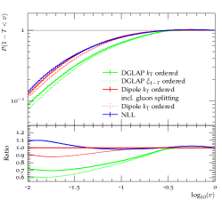
(a)  Thrust

(b)  BKS_1/2

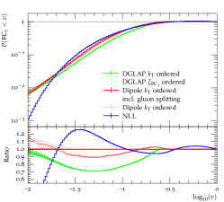
(c)  FC₁

Figure 7: Comparison between plain DGLAP parton shower ordered in $\xi$ to DGLAP parton shower ordered in dipole-$k_{T}$ and dipole shower with and without gluon splitting.

Figure 8 displays a cross-check on the logarithmic terms implemented by the dipole shower as compared to the parton shower and the analytic result. We extract $R(k_{T}/Q)$ for a fixed value of the strong coupling, $\alpha_{s}=0.118$, using the technique described in Lönnblad (2013). The slope of the distribution corresponds to the leading logarithm, while the offset of the analytic result corresponds to the next-to-leading logarithm. Any parton- or dipole-shower prediction must approach the analytic result as $k_{T}\to 0$, which is verified by the convergence of the predictions at small $k_{T}$.

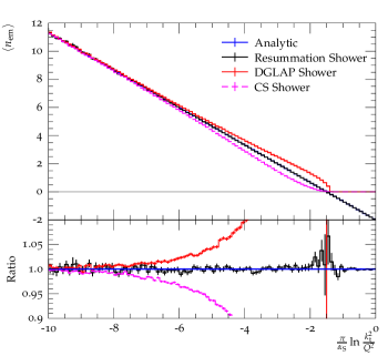
Figure 8: Comparison of analytic and parton-shower predictions for the emission probabilities in Eqs. (10) and  (11). The plot shows the average number of emissions per bin as a proxy observable Lönnblad (2013).

VI Conclusions

We have performed a detailed comparison between pure NLL resummation and parton showers for additive observables in $e^{+}e^{-}$ annihilation to hadrons. We have isolated their differences, which can broadly be classified as related to probability or momentum conservation. While a different treatment of these effects leads to formally subleading corrections on the resummed prediction, it can have a numerically sizable impact (20% or more) in the region where experimental measurements are performed. Similar effects can reasonably be expected to arise in other observables, as well as in processes with hadronic initial states and with a more complicated color structure at the Born level. When comparing analytic resummation to parton showers it should be kept in mind that such differences may exist, in which case they should be taken into account as a systematic uncertainty. We have shown in a simple scenario that the differences can be assessed quantitatively by casting analytic resummation into a Markovian Monte-Carlo simulation and introducing momentum and probability conservation. Conversely, parton showers can be modified to violate momentum and probability conservation to reproduce pure NLL resummation. From the practical point of view this approach is disfavored, as it leads to numerically inefficient Monte-Carlo algorithms.

Appendix A Gluon Radiators

Although we only deal with radiation off quark lines in this study, we argue that the same conclusions hold for radiating gluons. The basic reasoning is that the Sudakov form factor, Eq. (6) is an alternative form of the equations in Höche and Prestel (2017) that holds for leading-order DGLAP splitting functions due to their symmetries. If we use the correct form of the Sudakov factor, then we can extend the lower integration boundary for $z$ to zero without encountering a singularity, and we obtain the correct collinear anomalous dimensions. The detailed argument is as follows.

While the DGLAP equations are schematically identical for initial and final state, their implementation in parton-shower programs usually differs between the two, owing to the fact that Monte-Carlo simulations are inclusive over final states. The evolution equations for the fragmentation functions $D_{a}(x,Q^{2})$ for parton of type $a$ to fragment into a hadron read

$$\frac{{\rm d}\,xD_{a}(x,t)}{{\rm d}\ln t}=\sum_{b=q,g}\int_{0}^{1}{\rm d}\tau\int_{0}^{1}{\rm d}z\,\frac{\alpha_{s}}{2\pi}\big{[}zP_{ab}(z)\big{]}_{+}\,\tau D_{b}(\tau,t)\,\delta(x-\tau z)\;,$$ (21)

where the $P_{ab}$ are the unregularized DGLAP evolution kernels, and where the plus prescription is defined such as to enforce the momentum sum rule:

$$\big{[}zP_{ab}(z)\big{]}_{+}=\lim\limits_{\varepsilon\to 0}\bigg{[}zP_{ab}(z)\,\Theta(1-z-\varepsilon)-\delta_{ab}\sum_{c\in\{q,g\}}\frac{\Theta(z-1+\varepsilon)}{\varepsilon}\int_{0}^{1-\varepsilon}{\rm d}\zeta\,\zeta\,P_{ac}(\zeta)\bigg{]}\;.$$ (22)

For finite $\varepsilon$, the endpoint subtraction in Eq. (22) can be interpreted as the approximate virtual plus unresolved real corrections, which are included in the parton shower because the Monte-Carlo algorithm naturally implements a unitarity constraint Jadach and Skrzypek (2004). For $0<\varepsilon\ll 1$, Eq. (21) changes to

$$\frac{1}{D_{a}(x,t)}\,\frac{{\rm d}D_{a}(x,t)}{{\rm d}\ln t}=-\sum_{c=q,g}\int_{0}^{1-\varepsilon}{\rm d}\zeta\,\zeta\,\frac{\alpha_{s}}{2\pi}P_{ac}(\zeta)\,+\sum_{b=q,g}\int_{x}^{1-\varepsilon}\frac{{\rm d}z}{z}\,\frac{\alpha_{s}}{2\pi}\,P_{ab}(z)\,\frac{D_{b}(x/z,t)}{D_{a}(x,t)}\;.$$ (23)

Using the Sudakov form factor

$$\Delta_{a}(t_{0},t)=\exp\bigg{\{}-\int_{t_{0}}^{t}\frac{{\rm d}\bar{t}}{\bar{t}}\sum_{c=q,g}\int_{0}^{1-\varepsilon}{\rm d}\zeta\,\zeta\,\frac{\alpha_{s}}{2\pi}P_{ac}(\zeta)\bigg{\}}$$ (24)

the generating function for splittings of parton $a$ is defined as

$$\mathcal{D}_{a}(x,t,\mu^{2})=D_{a}(x,t)\Delta_{a}(t,\mu^{2})\,.$$ (25)

Equation (23) can now be written in the simple form

$$\frac{{\rm d}\ln\mathcal{D}_{a}(x,t,\mu^{2})}{{\rm d}\ln t}=\sum_{b=q,g}\int_{x}^{1-\varepsilon}\frac{{\rm d}z}{z}\,\frac{\alpha_{s}}{2\pi}\,P_{ab}(z)\,\frac{D_{b}(x/z,t)}{D_{a}(x,t)}\;.$$ (26)

The generalization to an $n$-parton final state, $\vec{a}=\{a_{1},\ldots,a_{n}\}$, resolved at scale $t$ can be made in terms of fragmenting jet functions, $\mathcal{G}$ Procura and Stewart (2010); Jain et al. (2011). If we define the generating function for this state as $\mathcal{F}_{\vec{a}}(\vec{x},t,\mu^{2})$, we can formulate its evolution equation in terms of a sum of the right hand side of Eq. (26). For unconstrained evolution, we can use Eq. (23), to write the differential decay probability as

$$\begin{split}\frac{{\rm d}}{{\rm d}\ln t}\ln\bigg{(}\frac{\mathcal{F}_{\vec{a}}(\vec{x},t,\mu^{2})}{\prod_{j\in\rm FS}\mathcal{G}_{a_{j}}(x_{j},t)}\bigg{)}=&\sum_{j\in{\rm FS}}\sum_{b=q,g}\int_{0}^{1-\varepsilon}{\rm d}z\,z\,\frac{\alpha_{s}}{2\pi}\,P_{a_{j}b}(z)\;.\end{split}$$ (27)

Thus, as highlighted in Jadach and Skrzypek (2004), it is generally necessary to use the Sudakov factor, Eq. (24), in final-state parton shower evolution. At the leading order, the factor $\zeta$ in Eq. (24) simply replaces the commonly used symmetry factor for $g\to g$ splitting and it also accounts for the proper counting of the number of active flavors. However, this reasoning applies only if the boundaries of the $\zeta$-integration are defined by momentum conservation, and are therefore symmetric around $\zeta=1/2$. In our analysis we attempt to extend the lower integration limit to zero, which would generate a spurious singularity arising from the symmetry of the gluon splitting function. Therefore, the commonly used technique of implementing the symmetrized gluon splitting function without an additional factor $\zeta$ cannot be used, and the only correct way to treat the problem is to work with Eq. (24).

Appendix B Analytic results at NLL accuracy

This section summarizes the components of the C AESAR formalism Banfi et al. (2005) that are needed for our analysis. The resummed cumulative cross section at NLL is given in this formalism by $\Sigma_{\rm NLL}(v)=e^{-R_{\rm NLL}(Q^{2},v)}\mathcal{F}(v)$, cf. Eq. (13). The unregularized branching probability $R(v)$ follows from Eq. (11). It is typically written in terms of $\lambda=\alpha_{s}\beta_{0}L$, where $L=-\ln v$. One obtains

$$R(v)=2C_{F}\left(r(L)+B_{q}T\left(\frac{L}{a+b}\right)\right)\;,$$ (28)

where $r(L)$ is separated into a leading and a sub-leading logarithmic piece as $r(L)=Lr_{1}(\alpha_{s}L)+r_{2}(\alpha_{s}L)$.

$$\begin{split}r_{1}(\alpha_{s}L)=&\;\frac{1}{2\pi\beta_{0}\lambda b}\left((a-2\lambda)\ln\left(1-\frac{2\lambda}{a}\right)-(a+b-2\lambda)\ln\left(1-\frac{2\lambda}{a+b}\right)\right)\;,\\ r_{2}(\alpha_{s}L)=&\;\frac{1}{b}\bigg{(}\frac{K}{(2\pi\beta_{0})^{2}}\left((a+b)\ln\left(1-\frac{2\lambda}{a+b}\right)-a\ln\left(1-\frac{2\lambda}{a}\right)\right)\\ &\qquad+\frac{\beta_{1}}{2\pi\beta_{0}^{3}}\bigg{(}\frac{a}{2}\ln^{2}\left(1-\frac{2\lambda}{a}\right)-\frac{a+b}{2}\ln^{2}\left(1-\frac{2\lambda}{a+b}\right)\\ &\qquad\qquad\qquad+a\ln\left(1-\frac{2\lambda}{a}\right)-(a+b)\ln\left(1-\frac{2\lambda}{a+b}\right)\bigg{)}\bigg{)}\;.\end{split}$$ (29)

The beta function coefficients and the two-loop cusp anomalous dimension in the $\overline{\rm MS}$ scheme are given by

$$\begin{split}\beta_{0}=&\;\frac{1}{2\pi}\left(\frac{11}{6}C_{A}-\frac{2}{3}T_{R}n_{f}\right)\;,\\ \beta_{1}=&\;\frac{1}{(2\pi)^{2}}\left(\frac{17}{6}C_{A}^{2}-\left(\frac{5}{3}C_{A}+C_{F}\right)T_{R}n_{f}\right)\;,\\ K=&\;\left(\frac{67}{18}-\frac{\pi^{2}}{6}\right)C_{A}-\frac{10}{9}T_{R}n_{f}\;.\end{split}$$ (30)

The sub-leading logarithmic term $T(L)$ is defined as

$$T(L)=\int_{Q^{2}e^{-2L}}^{Q^{2}}\frac{dk_{T}^{2}}{k_{T}^{2}}\frac{\alpha_{s}(k_{T}^{2})}{\pi}=-\frac{1}{\pi\beta_{0}}\ln(1-2\lambda)\;.$$ (31)

The $\mathcal{F}$-function, Eq. (14), for additive observables is given by

$$\mathcal{F}(v)=\frac{e^{-\gamma_{E}R^{\prime}(v)}}{\Gamma(1+R^{\prime}(v))}\;.$$ (32)

Since both $T(L)$ and $r_{2}(L)$ are sub-leading in $L$, we have

$$R^{\prime}(v)=2C_{F}\,r^{\prime}(L)\;,\qquad\text{where}\qquad r^{\prime}(L)=r_{1}^{\prime}(L)=\frac{1}{b}\left(T\left(\frac{L}{a}\right)-T\left(\frac{L}{a+b}\right)\right)\;.$$ (33)

Using Eq. (33) it can be verified that the combination of $z_{<v,\rm soft}^{\rm max}$ and $\mu_{<v,\rm soft}^{2}$ listed in Tab. 1 generates the correct value of $r^{\prime}(L)$, and therefore the correct value of the $\mathcal{F}$-function.

Appendix C Definition of observables

This appendix summarizes the definitions of observables used in our study and lists their parametrizations in terms of the coefficients $a$ and $b$ in Eq. (2). Note that $\vec{q}_{i}$ stands for any momentum in the event, no matter if this momentum is hard or soft.

The thrust observable for arbitrary $e^{+}e^{-}$ events is defined as Farhi (1977)

$$\tau=1-\max_{\vec{n}}\frac{\sum_{i}|\vec{q}_{i}\vec{n}|}{\sum_{i}|\vec{q}_{i}|}\;.$$ (34)

The maximization procedure defines a unit vector, $\vec{n}_{T}$, which is referred to as the thrust axis. In the 2-jet limit, Eq. (34) can be written as

$$\tau=\min_{\vec{n}}\frac{\sum_{i}|\vec{q}_{i}|(1-|\cos\theta_{i}|)}{\sum_{i}|\vec{q}_{i}|}\;,$$ (35)

where $\theta_{i}$ are the angles of the momenta with respect to $\vec{n}_{T}$. The coefficients in Eq. (2) are given by $a=b=1$ Banfi et al. (2005).

The BKS observable is defined as Berger et al. (2003a, b)

$${\rm BKS}_{x}=\frac{\sum_{i}E_{i}|\sin\theta_{i}|^{x}(1-|\cos\theta_{i}|)^{1-x}}{\sum_{i}|\vec{q}_{i}|}\;,$$ (36)

where $\theta_{i}$ are again the angles of the momenta with respect to the thrust axis. For this study we set $x=1/2$, which implies $a=1$ and $b=1/2$ Banfi et al. (2005).

The fractional energy correlation is defined as Banfi et al. (2005)

$${\rm FC}_{x}=\sum_{i\neq j}\frac{E_{i}E_{j}|\sin\theta_{ij}|^{x}(1-|\cos\theta_{ij}|)^{1-x}}{(\sum_{i}E_{i})^{2}}\Theta\big{(}(\vec{q}_{i}\vec{n}_{T})(\vec{q}_{j}\vec{n}_{T})\big{)}\;,$$ (37)

where $\vec{n}_{T}$ is the thrust axis. For this study we set $x=1$, which implies $a=1$ and $b=0$ Banfi et al. (2005).

References

- Dokshitzer et al. (1980) Y. L. Dokshitzer, D. Diakonov, and S. I. Troian, Phys. Rept. 58, 269 (1980).
- Parisi and Petronzio (1979) G. Parisi and R. Petronzio, Nucl. Phys. B154, 427 (1979).
- Collins and Soper (1981) J. C. Collins and D. E. Soper, Nucl. Phys. B193, 381 (1981).
- Sterman (1987) G. F. Sterman, Nucl. Phys. B281, 310 (1987).
- Catani and Trentadue (1989) S. Catani and L. Trentadue, Nucl. Phys. B327, 323 (1989).
- Catani and Trentadue (1991) S. Catani and L. Trentadue, Nucl. Phys. B353, 183 (1991).
- Catani et al. (1993) S. Catani, L. Trentadue, G. Turnock, and B. R. Webber, Nucl. Phys. B407, 3 (1993).
- Catani et al. (2000) S. Catani et al., in 1999 CERN Workshop on SM physics (and more) at the LHC (2000) hep-ph/0005025 .
- Dissertori et al. (2009) G. Dissertori et al., JHEP 08, 036 (2009), arXiv:0906.3436 [hep-ph] .
- Gehrmann et al. (2010) T. Gehrmann, M. Jaquier, and G. Luisoni, Eur. Phys. J. C67, 57 (2010), arXiv:0911.2422 [hep-ph] .
- Bauer et al. (2002a) C. W. Bauer, D. Pirjol, and I. W. Stewart, Phys.Rev. D65, 054022 (2002a), hep-ph/0109045 .
- Bauer et al. (2002b) C. W. Bauer, S. Fleming, D. Pirjol, I. Z. Rothstein, and I. W. Stewart, Phys.Rev. D66, 014017 (2002b), hep-ph/0202088 .
- Kidonakis and Sterman (1997) N. Kidonakis and G. F. Sterman, Nucl. Phys. B505, 321 (1997), hep-ph/9705234 .
- Kidonakis et al. (1998a) N. Kidonakis, G. Oderda, and G. F. Sterman, Nucl.Phys. B531, 365 (1998a), hep-ph/9803241 .
- Laenen et al. (1998) E. Laenen, G. Oderda, and G. F. Sterman, Phys. Lett. B438, 173 (1998), hep-ph/9806467 .
- Bonciani et al. (2003) R. Bonciani, S. Catani, M. L. Mangano, and P. Nason, Phys. Lett. B575, 268 (2003), hep-ph/0307035 .
- Banfi et al. (2002) A. Banfi, G. Salam, and G. Zanderighi, JHEP 01, 018 (2002), hep-ph/0112156 .
- Banfi et al. (2005) A. Banfi, G. P. Salam, and G. Zanderighi, JHEP 03, 073 (2005), hep-ph/0407286 .
- Banfi et al. (2015) A. Banfi, H. McAslan, P. F. Monni, and G. Zanderighi, JHEP 05, 102 (2015), arXiv:1412.2126 [hep-ph] .
- Gerwick et al. (2014) E. Gerwick, S. Höche, S. Marzani, and S. Schumann, (2014), arXiv:1411.7325 [hep-ph] .
- Fox and Wolfram (1980) G. C. Fox and S. Wolfram, Nucl. Phys. B168, 285 (1980).
- Marchesini and Webber (1984) G. Marchesini and B. R. Webber, Nucl. Phys. B238, 1 (1984).
- Sjöstrand (1985) T. Sjöstrand, Phys. Lett. B157, 321 (1985).
- Marchesini and Webber (1988) G. Marchesini and B. R. Webber, Nucl. Phys. B310, 461 (1988).
- Catani et al. (1991) S. Catani, B. R. Webber, and G. Marchesini, Nucl. Phys. B349, 635 (1991).
- Gribov and Lipatov (1972) V. N. Gribov and L. N. Lipatov, Sov. J. Nucl. Phys. 15, 438 (1972).
- Lipatov (1975) L. N. Lipatov, Sov. J. Nucl. Phys. 20, 94 (1975).
- Dokshitzer (1977) Y. L. Dokshitzer, Sov. Phys. JETP 46, 641 (1977).
- Altarelli and Parisi (1977) G. Altarelli and G. Parisi, Nucl. Phys. B126, 298 (1977).
- Amati et al. (1980) D. Amati, A. Bassetto, M. Ciafaloni, G. Marchesini, and G. Veneziano, Nucl. Phys. B173, 429 (1980).
- Botts and Sterman (1989) J. Botts and G. F. Sterman, Nucl.Phys. B325, 62 (1989).
- Kidonakis and Sterman (1996) N. Kidonakis and G. F. Sterman, Phys.Lett. B387, 867 (1996).
- Kidonakis et al. (1998b) N. Kidonakis, G. Oderda, and G. F. Sterman, Nucl. Phys. B525, 299 (1998b), hep-ph/9801268 .
- Oderda (2000) G. Oderda, Phys. Rev. D61, 014004 (2000), hep-ph/9903240 .
- Kidonakis and Owens (2001) N. Kidonakis and J. Owens, Phys.Rev. D63, 054019 (2001), hep-ph/0007268 .
- Dasgupta and Salam (2001) M. Dasgupta and G. Salam, Phys.Lett. B512, 323 (2001), hep-ph/0104277 .
- Höche et al. (2010) S. Höche, S. Schumann, and F. Siegert, Phys. Rev. D81, 034026 (2010), arXiv:0912.3501 [hep-ph] .
- Lönnblad (2013) L. Lönnblad, Eur.Phys.J. C73, 2350 (2013), arXiv:1211.7204 [hep-ph] .
- Farhi (1977) E. Farhi, Phys. Rev. Lett. 39, 1587 (1977).
- Berger et al. (2003a) C. F. Berger, T. Kucs, and G. F. Sterman, Int. J. Mod. Phys. A18, 4159 (2003a), hep-ph/0212343 .
- Berger et al. (2003b) C. F. Berger, T. Kucs, and G. F. Sterman, Phys. Rev. D68, 014012 (2003b), hep-ph/0303051 .
- Höche (2015) S. Höche, in Proceedings of TASI 2014 (2015) pp. 235–295, arXiv:1411.4085 [hep-ph] .
- Catani and Seymour (1997) S. Catani and M. H. Seymour, Nucl. Phys. B485, 291 (1997), hep-ph/9605323 .
- Höche and Prestel (2015) S. Höche and S. Prestel, Eur. Phys. J. C75, 461 (2015), arXiv:1506.05057 [hep-ph] .
- Ellis et al. (1981) R. Ellis, D. Ross, and A. Terrano, Nucl. Phys. B178, 421 (1981).
- Höche and Prestel (2017) S. Höche and S. Prestel, Phys. Rev. D96, 074017 (2017), arXiv:1705.00742 [hep-ph] .
- Jadach and Skrzypek (2004) S. Jadach and M. Skrzypek, Acta Phys. Polon. B35, 745 (2004), arXiv:hep-ph/0312355 [hep-ph] .
- Procura and Stewart (2010) M. Procura and I. W. Stewart, Phys. Rev. D81, 074009 (2010), arXiv:0911.4980 [hep-ph] .
- Jain et al. (2011) A. Jain, M. Procura, and W. J. Waalewijn, JHEP 05, 035 (2011), arXiv:1101.4953 [hep-ph] .