Individual eigenvalue distributions of crossover chiral random matrices and low-energy constants of SU(2)$\times$U(1) lattice gauge theory

Abstract

We compute individual distributions of low-lying eigenvalues of a chiral random matrix ensemble interpolating symplectic and unitary symmetry classes by the Nyström-type method of evaluating the Fredholm Pfaffian and resolvents of the quaternion kernel. The one-parameter family of these distributions is shown to fit excellently the Dirac spectra of SU(2) lattice gauge theory with a constant U(1) background or dynamically fluctuating U(1) gauge field, which weakly breaks the pseudoreality of the unperturbed SU(2) Dirac operator. The observed linear dependence of the crossover parameter with the strength of the U(1) perturbations leads to precise determination of the pseudo-scalar decay constant, as well as the chiral condensate in the effective chiral Lagrangian of the AI class.

B01,B60,B64,B83,B86

1 Introduction

The grounds for universality, i.e., insensitivity to details of the system of concern, of local correlation of energy levels of stochastic and quantum-chaotic Hamiltonians have been well uncovered by now, in terms of ten-fold classification of symmetric superspaces on which spectral nonlinear $\sigma$ models describing spontaneous symmetry breaking reside Zir96 , and of semiclassical equivalence between periodic orbits and the aforementioned $\sigma$ models MHABH09 . On the other hand, the presence of explicit symmetry breaking perturbations is known to induce a crossover between different universality classes Dys62 , in such a way that is also insensitive to the systems’ details. An example of this universality crossover is the Gaussian orthogonal ensemble (GOE)–Gaussian unitary ensemble (GUE) transition in a disordered or chaotic system under a magnetic field DM91 ; SNMB09 . In the realm of lattice gauge theory, where Dirac operators play the rôle of stochastic Hamiltonians SV93 ; Ver94 , the crossover between the chiral Gaussian unitary ensemble (chGUE) itself and the chGUE–GUE crossover, associated with an imaginary isospin chemical potential DHSS05 and a finite lattice-spacing effect in the Wilson Dirac operator DSV10 , respectively, have been utilized to determine the pion decay constant and the Wilsonian chiral perturbation constants from relatively small lattices. The aim of this work is to apply this spectral approach to the determination of low-energy constants in another setting, namely SU(2) gauge theory under U(1) perturbations, either in the form of a constant imaginary chemical potential Nis12-1 ; Nis12-2 or a dynamically fluctuating one. In contrast to these preceding works which used $n$-level correlation functions or the smallest eigenvalue distribution, our strategy in this paper is to employ multiple spectral observables which allows for precise fitting of lattice data, namely, individual distributions of the $k$th smallest Dirac eigenvalues DN01 inclusively. The practical advantages of our method will be proved in the precision of the low-energy constants determined, as preliminarily reported in Ref. NY14 .

This paper is composed mainly of two parts: Sect. 2 is devoted to analytic treatments in random matrix theory, and Sect. 3 to its application to Dirac eigenvalue distributions measured in lattice simulations. In Sect. 2 we start by reviewing the established results of the chiral Gaussian symplectic ensemble (chGSE)–chGUE crossover, namely, the derivation of the quaternion kernel $K$ FNH99 ; NF99 ; Nag05 . Then we apply the Nyström-type method Bor10-1 ; Bor10-2 to that kernel and compute individual eigenvalue distributions in the form of the Fredholm Pfaffian and resolvents of $\hat{K}$ Nis15 . The relationship between the chiral Lagrangian in the $\varepsilon$ regime and the nonlinear $\sigma$ model from random matrices interpolating chGSE–chGUE leads to identification between parameters in each theory. In Sect. 3 we introduce our models of lattice gauge theory and explain our strategy of fitting the Dirac spectra using individual eigenvalue distributions of chGSE and of the chGSE–chGUE crossover. Optimally fitting parameters (mean level spacings $\varDelta$ and crossover parameters $\rho$) will be exhibited in Tables 1–6, leading to very precise determination of the low-energy constants (chiral condensate $\Sigma$ and pseudo-scalar decay constant $F$) as presented in Table 7. Our conclusions, including a possible direction of study, will be summarized in Sect. 4.

2 chGSE–chGUE crossover

2.1 Crossover random matrix ensemble

Let $N$ and $N^{\prime}$ be even positive integers. Let $\boldsymbol{\mathit{A}}$ and $\boldsymbol{\mathit{B}}$ be $(N/2)\times(N^{\prime}/2)$ quaternion matrices, which can be represented as ordinary $N\times N^{\prime}$ matrices $A$ and $B$ as

$$A=\sum_{\mu=0}^{3}\left(A^{(\mu)}_{jk}\right)\otimes\sigma_{\mu},\ \ B=\sum_{\mu=0}^{3}\left(B^{(\mu)}_{jk}\right)\otimes\sigma_{\mu}\ \ (j=1,\ldots,N/2,\ k=1,\ldots,N^{\prime}/2).$$ (1)

Here the four units of the quaternion field $\mathbb{H}$ are represented by the $2\times 2$ unit matrix and Pauli matrices, $\{\sigma_{\mu}\}=(\mathbb{I},-i\sigma_{1},-i\sigma_{2},-i\sigma_{3})$. Let these matrix elements belong to

$$A^{(\mu)}_{jk}\in\mathbb{R},\ B^{(\mu)}_{jk}\in\mathbb{C},$$ (2)

i.e., $\boldsymbol{\mathit{A}}$ is quaternion-real and $\boldsymbol{\mathit{B}}$ is not (i.e., $B$ is a generic $N\times N^{\prime}$ complex matrix). We consider $A^{(\mu)}_{jk}$, ${\rm Re}\,B^{(\mu)}_{jk}$, and ${\rm Im}\,B^{(\mu)}_{jk}$ to be independent random variables, distributed according to the Gaussian distributions $e^{-\frac{1}{2}{\rm tr}\,AA^{\dagger}}$ and $e^{-{\rm tr}\,BB^{\dagger}}$, respectively. We define an ensemble of $(N+N^{\prime})\times(N+N^{\prime})$ Hermitian matrices $H$ of the form

$$H=\left[\begin{array}[]{cc}0_{N\times N}&C\\ C^{\dagger}&0_{N^{\prime}\times N^{\prime}}\end{array}\right],\ \ C=e^{-\tau}A+\sqrt{1-e^{-2\tau}}B,$$ (3)

where $\tau$ is a real parameter, initially introduced by Dyson as a fictitious time for the Brownian motion of eigenvalues Dys62 . This ensemble is called a “chiral” random matrix ensemble because it enjoys the chiral symmetry $\left\{H,\gamma_{5}\right\}=0$ with $\gamma_{5}={\rm diag}(\mathbb{I}_{N},-\mathbb{I}_{N^{\prime}})$. This anticommutation relation implies that the eigenvalues of $H$ consist of $\min(N^{\prime},N)$ pairs of generically nonzero eigenvalues of equal magnitude and opposite signs (i.e., $(\pm 1)\times$ singular values of $C$), and $\nu=|N^{\prime}-N|$ zero eigenvalues. The presence of $B$ violates the quaternion-reality of $\boldsymbol{\mathit{C}}$ and the self-duality of $H$ (i.e.,  $H_{ij}^{(\mu)}\otimes\sigma_{\mu}=H_{ji}^{(\mu)}\otimes\sigma_{\mu}^{\dagger},\ i,j=1,\ldots,N+N^{\prime}$), and lifts the Kramers degeneracy of all nonzero eigenvalues of $H$ (i.e.,  singular values of $A$ alone). Accordingly, this random matrix ensemble interpolates between two limiting cases, the chiral Gaussian Symplectic Ensemble (chGSE) at $\tau=0$ and the chiral Gaussian Unitary Ensemble (chGUE) at $\tau\to\infty$, depending on a single parameter $\tau$ (at a fixed, finite $N$ and $N^{\prime}$).

2.2 Joint eigenvalue distribution

In order to make the paper self-contained, below we sketch the derivation of the probability distribution of singular values of $C$, and refer the reader to Refs. FNH99 ; NF99 ; Nag05 for rigorous proofs of the relevant formulas. We start from the unnormalized probability measure of the matrix elements of $C$,

$$dC\,\int dA\,e^{-\frac{1}{2}{\rm tr}\,AA^{\dagger}}\int dB\,e^{-{\rm tr}\,BB^{\dagger}}\delta(e^{-\tau}A+\sqrt{1-e^{-2\tau}}B-C)$$ (4)

$$\propto dC\,\int dA\,\exp\left(-\frac{1}{2}{\rm tr}\,AA^{\dagger}-\frac{1}{1-e^{-2\tau}}{\rm tr}\,(C-e^{-\tau}A)(C-e^{-\tau}A)^{\dagger}\right),$$

where $dA=\prod_{j,k,\mu}dA_{jk}^{(\mu)}$, $dB=\prod_{j,k,\mu}d^{2}B_{jk}^{(\mu)}$, and $dC=\prod_{j,k,\mu}d^{2}C_{jk}^{(\mu)}$. Without loss of generality we assume $N\leq N^{\prime}$. We employ the singular value decomposition $A=SMS^{\prime}{}^{\dagger}$ and $C=U\Lambda U^{\prime}{}^{\dagger}$ with $S\in{\rm USp}(N),S^{\prime}\in{\rm USp}(N^{\prime}),U\in{\rm U}(N),U^{\prime}\in{\rm U}(N^{\prime})$ and parametrize the singular values as $M=\Bigl{[}{\rm diag}\left(\mu_{1},\ldots,\mu_{N}\right)\ 0_{N\times\nu}\Bigr{]},\ \Lambda=\Bigl{[}{\rm diag}\left(\lambda_{1},\ldots,\lambda_{N}\right)\ 0_{N\times\nu}\Bigr{]}$. Kramers-degenerate pairs of singular values of $A$ are ordered such that $\mu_{i+N/2}=\mu_{i}\ (i=1,\ldots,N/2)$. The measures $dA$ and $dB$ on quaternion-real matrices and complex matrices take the following respective forms (in what follows we suppress all constant factors in the measures):

$$dA=d(S,S^{\prime})\left(\prod_{i=1}^{N/2}d\mu_{i}\,\mu_{i}^{2\nu+3}\right)\triangle_{N/2}(\mu^{2})^{4},\ \ dC=d(U,U^{\prime})\left(\prod_{i=1}^{N}d\lambda_{i}\,\lambda_{i}^{2\nu+1}\right)\triangle_{N}(\lambda^{2})^{2}.$$ (5)

Here $d(S,S^{\prime})$ and $d(U,U^{\prime})$ denote the invariant measures on the respective angular degrees of freedom, and $\triangle$ denote the Vandermonde determinants $\triangle_{N/2}(\mu^{2}):=\prod_{i>j}^{N/2}(\mu_{i}^{2}-\mu_{j}^{2})$ and $\triangle_{N}(\lambda^{2}):=\prod_{i>j}^{N}(\lambda_{i}^{2}-\lambda_{j}^{2})$. The probability measure of the singular values $\{\lambda_{i}\}$ of $C$ follows from Eqs. (4) and (5) by integrating out the unitary matrices $(U,U^{\prime})$. The integrations over symplectic matrices $(S,S^{\prime})$ decouple after redefining the unitary matrices by $S^{\dagger}U\to U$ and $S^{\prime}{}^{\dagger}U^{\prime}\to U^{\prime}$, leading to the expression

$$\text{Eq.}(\ref{dC}) = \prod_{i=1}^{N}d\lambda_{i}\,\lambda_{i}^{2\nu+1}\,\exp\left(-\frac{\lambda_{i}^{2}}{1-e^{-2\tau}}\right)\triangle_{N}(\lambda^{2})^{2}\int_{0}^{\infty}\prod_{j=1}^{N/2}d\mu_{j}\,\mu_{j}^{2\nu+3}\,\exp\left(-\frac{\mu_{j}^{2}}{\tanh\tau}\right)$$ (6)

$$\times\triangle_{N/2}(\mu^{2})^{4}\int_{{\rm U}(N)}\!\!\!\!\!\!\!dU\int_{{\rm U}(N^{\prime})}\!\!\!\!\!\!\!\!\!dU^{\prime}\ \exp\left(\frac{1}{\sinh\tau}{\rm Re}\,{\rm tr}\,U\Lambda U^{\prime}{}^{\dagger}M^{t}\right).$$

We employ the Berezin–Karpelevich formula BK68 ; GW96 ; JSV96 for the integration over $(U,U^{\prime})$ and take the pairwise confluent limit $\mu_{i+N/2}\to\mu_{i}$ for all $i=1,\ldots,N/2$:

$$\int_{{\rm U}(N)}\!\!\!\!\!\!\!\!dU\int_{{\rm U}(N^{\prime})}\!\!\!\!\!\!\!\!\!\!dU^{\prime}\ \;\,e^{\frac{1}{\sinh\tau}{\rm Re}\,{\rm tr}\,U\Lambda U^{\prime}{}^{\dagger}M^{t}} \propto \left.\frac{\det\left[I_{\nu}\left(\frac{\lambda_{i}\mu_{j}}{\sinh\tau}\right)\right]_{i,j=1}^{N}}{\triangle_{N}(\lambda^{2})\triangle_{N}(\mu^{2})\prod_{i=1}^{N}(\lambda_{i}\mu_{i})^{\nu}}\right|_{\mu_{i+N/2}\to\mu_{i}}$$ (7)

$$\propto \frac{\det\left[I_{\nu}\left(\frac{\lambda_{i}\mu_{j}}{\sinh\tau}\right)\ \frac{\partial}{\partial\mu_{j}^{2}}I_{\nu}\left(\frac{\lambda_{i}\mu_{j}}{\sinh\tau}\right)\right]_{i=1,\ldots,N}^{j=1,\ldots,N/2}}{\triangle_{N}(\lambda^{2})\triangle_{N/2}(\mu^{2})^{4}\prod_{i=1}^{N}\lambda_{i}^{\nu}\prod_{j=1}^{N/2}\mu_{j}^{2\nu}}.$$

Here $I_{\nu}$ denotes the Bessel function of the pure imaginary argument, $I_{\nu}(z)=J_{\nu}(iz)$. By substituting Eq. (7) into Eq. (6) and performing a change of variables from the singular values of rectangular matrices $C$ and $A$ to the eigenvalues of Wishart matrices $CC^{\dagger}$ and $AA^{\dagger}$, $x_{i}=\lambda_{i}^{2}$ and $y_{i}=\mu_{i}^{2}$, the probability measure becomes proportional to

$$\text{Eq.}(\ref{dlambda})\ \propto\ \prod_{i=1}^{N}dx_{i}\,\sqrt{w(x_{i})}\,\triangle_{N}(x)\int_{0}^{\infty}\prod_{j=1}^{N/2}dy_{j}\,y_{j}\det\left[g(x_{k},y_{\ell})\ \ \frac{\partial g(x_{k},y_{\ell})}{\partial y_{\ell}}\right]^{k=1,\ldots,N}_{\ell=1,\ldots,N/2}.$$ (8)

Here we have introduced the Laguerre weight $w(x):=x^{\nu}e^{-x}$, and the symmetric function

$$g(x,y):=\frac{e^{-(2\nu+1)\tau}}{1-e^{-2\tau}}\exp\left(-\frac{x+y}{2\tanh\tau}\right)I_{\nu}\left(\frac{\sqrt{xy}}{\sinh\tau}\right).$$ (9)

With the multiplicative constant chosen as the above, the function $g(x,y)$ admits an alternative interpretation as a one-particle Green’s function for the Brownian motion at time $\tau$,

$$g(x,y)=\sqrt{w(x)w(y)}\sum_{k=0}^{\infty}\frac{L_{k}^{\nu}(x)L_{k}^{\nu}(y)}{h_{k}}e^{-\gamma_{k}\tau},$$ (10)

with the norm given by $h_{k}={(k+\nu)!}/{k!}$ and the “one-particle energy” by $\gamma_{k}=2k+\nu+1$. Using a lemma by Mehta (A.17 of Ref. Meh04 ), the $(N/2)$-fold integral of an $N\times N$ determinant in Eq. (8) can be decomposed into an $N\times N$ Pfaffian of single integrals:

$$\text{Eq.}(\ref{dlambda2}) \propto \prod_{i=1}^{N}dx_{i}\,\sqrt{w(x_{i})}\,\triangle_{N}(x)\,{\rm Pf}\left[F(x_{j},x_{k})\right]_{j,k=1,\ldots,N},$$ (11)

$$F(x,x^{\prime}) := \int_{0}^{\infty}dy\,y\left\{g(x,y)\frac{\partial g(x^{\prime},y)}{\partial y}-\frac{\partial g(x,y)}{\partial y}g(x^{\prime},y)\right\}.$$ (12)

2.3 Quaternion determinant

In this subsection we summarize the procedure presented in Ref. Meh04 , Sect. 14. We introduce a set of arbitrary monic polynomials $\{R_{k}(x)\}_{k=0,1,\ldots}$ and arbitrary positive numbers $\{r_{k}\}_{k=0,1,\ldots}$, and define functions $\{\psi_{k}(x)\}$ by

$$\psi_{2k}(x)=\frac{\sqrt{w(x)}R_{2k}(x)}{\sqrt{r_{k}}},\quad\psi_{2k+1}(x)=\frac{\sqrt{w(x)}R_{2k+1}(x)}{\sqrt{r_{k}}}$$ (13)

and their $F$-convolutions $\{\phi_{k}(x)\}$ by

$$\phi_{k}(x)=-\int_{0}^{\infty}dx^{\prime}\,F(x,x^{\prime})\psi_{k}(x^{\prime}).$$ (14)

Next we introduce functions $D(x,x^{\prime})$, $S(x,x^{\prime})$, and $I(x,x^{\prime})$, which are bilinear combinations of $\{\psi_{k}(x)\}$ and $\{\phi_{k}(x)\}$:

$$D(x,x^{\prime}) = \sum_{k=0}^{N/2-1}\Bigl{(}\psi_{2k}(x)\psi_{2k+1}(x^{\prime})-\psi_{2k+1}(x)\psi_{2k}(x^{\prime})\Bigr{)},$$ (15)

$$S(x,x^{\prime}) = \sum_{k=0}^{N/2-1}\Bigl{(}\phi_{2k}(x)\psi_{2k+1}(x^{\prime})-\phi_{2k+1}(x)\psi_{2k}(x^{\prime})\Bigr{)},$$ (16)

$$I(x,x^{\prime}) = -\sum_{k=0}^{N/2-1}\Bigl{(}\phi_{2k}(x)\phi_{2k+1}(x^{\prime})-\phi_{2k+1}(x)\phi_{2k}(x^{\prime})\Bigr{)},$$ (17)

and the corresponding $N\times N$ matrices $D_{N}$, $S_{N}$, and $I_{N}$ by

$${D}_{N}=[D(x_{i},x_{j})]_{i,j=1,\ldots,N},\ {S}_{N}=[S(x_{i},x_{j})]_{i,j=1,\ldots,N},\ {I}_{N}=[I(x_{i},x_{j})]_{i,j=1,\ldots,N}.$$ (18)

Since a $2N\times 2N$ antisymmetric matrix $\left[\begin{array}[]{cc}D_{N}&S_{N}{}^{t}\\ -S_{N}&-I_{N}\end{array}\right]$ is a product of two rectangular matrices of size $2N\times N$ and $N\times 2N$:

$$\left[\begin{array}[]{cc}D_{N}&S_{N}{}^{t}\\ -S_{N}&-I_{N}\end{array}\right]=\left[\begin{array}[]{cc}\psi_{2k}(x_{i})&\psi_{2k+1}(x_{i})\\ -\phi_{2k}(x_{i})&-\phi_{2k+1}(x_{i})\end{array}\right]^{i=1,\ldots,N}_{k=0,\ldots,N/2-1}\left[\begin{array}[]{cc}\psi_{2k+1}(x_{j})&-\phi_{2k+1}(x_{j})\\ -\psi_{2k}(x_{j})&\phi_{2k}(x_{j})\end{array}\right]_{j=1,\ldots,N}^{k=0,\ldots,N/2-1},$$

its rank is $N$ at most; and also it is $N$ at least due to the linear independence of $\{\psi_{i}(x)\}_{i=0,\ldots,N-1}$. Accordingly the lower $N$ rows $\left[-S_{N}\ -I_{N}\right]$ are linear combinations of the upper $N$ rows $\left[D_{N}\ S_{N}{}^{t}\right]$. Now consider a Pfaffian of another antisymmetric $2N\times 2N$ matrix $\left[\begin{array}[]{cc}D_{N}&S_{N}{}^{t}\\ -S_{N}&-I_{N}-F_{N}\end{array}\right]$ with ${F}_{N}=[F(x_{i},x_{j})]_{i,j=1,\ldots,N}$. Since adding $\left[S_{N}\ I_{N}\right]$ (or minus its transpose) to the lower $N$ rows (the right $N$ columns) does not change the determinants due to the aforementioned linear dependence with the upper $N$ rows (the left $N$ columns), we readily obtain

$${\rm Pf}\left[\begin{array}[]{cc}D_{N}&S_{N}{}^{t}\\ -S_{N}&-I_{N}-F_{N}\end{array}\right]={\rm Pf}\left[\begin{array}[]{cc}D_{N}&0\\ 0&-F_{N}\end{array}\right]=(-1)^{N/2}\,{\rm Pf}\,D_{N}\cdot{\rm Pf}\,F_{N}.$$ (19)

On the other hand,

$${\rm Pf}\,D_{N}={\rm Pf}\,\left[\left[\psi_{2k}(x_{i})\ \psi_{2k+1}(x_{i})\right]^{i=1,\ldots,N}_{k=0,\ldots,N/2-1}\left[\begin{array}[]{c}\psi_{2k+1}(x_{j})\\ -\psi_{2k}(x_{j})\end{array}\right]^{k=0,\ldots,N/2-1}_{j=1,\ldots,N}\right]$$ (22)

$$=\det\left[\psi_{k-1}(x_{i})\right]_{i,k=1,\ldots,N}=\det\left[\sqrt{w(x_{i})}x_{i}^{k-1}\right]_{i,k=1,\ldots,N}\propto\prod_{i=1}^{N}\sqrt{w(x_{i})}\cdot\triangle_{N}(x).$$ (23)

Using Eqs. (19) and (23), the probability measure (11) now reads

$$\text{Eq.}(\ref{dlambda3})\ \propto\ \prod_{i=1}^{N}dx_{i}\,{\rm Pf}\left(ZK_{N}\right),$$ (24)

$$K_{N}=\left[\begin{array}[]{cc}S_{N}&J_{N}\\ D_{N}&S_{N}{}^{t}\end{array}\right],\ \ J_{N}=I_{N}+F_{N},\ \ Z=\left[\begin{array}[]{cc}0&\mathbb{I}_{N}\\ -\mathbb{I}_{N}&0\end{array}\right].$$ (29)

Since its upper diagonal block is the transpose of the lower diagonal block and both off-diagonal blocks are antisymmetric, $K_{N}$ can be regarded a $2N\times 2N$ complex matrix representative of an $N\times N$ quaternion self-dual matrix, which we call $\boldsymbol{\mathit{K}}_{N}=[\boldsymbol{\mathit{K}}(x_{i},x_{j})]_{i,j=1,\ldots,N}$. Using Dyson’s lemma ${\rm qdet}\,\mathbf{\Phi}={\rm Pf}\,(Z\Phi)$ for the quaternion determinant (qdet) Dys70 of a quaternion self-dual matrix $\mathbf{\Phi}$, we finally obtain

$$\text{Eq.}(\ref{jpd6})=\prod_{i=1}^{N}dx_{i}\,{\rm qdet}\boldsymbol{\mathit{K}}_{N}(x_{1},\ldots,x_{N}).$$ (30)

2.4 Skew-orthogonal polynomials

We would like to choose $\{R_{k}(x)\}$ and $\{r_{k}\}$ (which are so far arbitrary) in such a way that the $2\times 2$ matrix $K(x,y)=\left[\begin{array}[]{cc}S(x,y)&J(x,y)\\ D(x,y)&S(y,x)\end{array}\right]$ representing the quaternion kernel $\boldsymbol{\mathit{K}}(x,y)$ enjoys the quasi-projectivity

$$\int_{0}^{\infty}dy\,{K}(x,y){K}(y,z)={K}(x,z)\left[\begin{array}[]{cc}1&0\\ 0&0\end{array}\right]+\left[\begin{array}[]{cc}0&0\\ 0&1\end{array}\right]{K}(x,z),$$ (31)

and is correctly normalized:

$$\int_{0}^{\infty}dx\,{K}(x,x)=N.$$ (32)

These two relationships would yield a crucial property that the restricted quaternion matrix $\boldsymbol{\mathit{K}}_{n}=[\boldsymbol{\mathit{K}}(x_{i},x_{j})]_{i,j=1,\ldots,n}$ satisfies the recursion relation

$$\int_{0}^{\infty}dx_{n}\,{\rm qdet}\,\boldsymbol{\mathit{K}}_{n}(x_{1},\ldots,x_{n})=(N-n+1)\,{\rm qdet}\,\boldsymbol{\mathit{K}}_{n-1}(x_{1},\ldots,x_{n-1}),$$ (33)

from which a $k$-level correlation function is expressed as $\mathrm{qdet}\,\boldsymbol{\mathit{K}}_{k}=\mathrm{Pf}(ZK_{k})$. It is well established that the properties (31), (32) are fulfilled by requiring $\{R_{k}(x)\}$ to be skew-orthogonal with respect to the skew inner product $\left\langle~{},~{}\right\rangle$ and $\{r_{k}\}$ to be their skew-norms,

$$\left\langle f,g\right\rangle:=\int_{0}^{\infty}dx\int_{0}^{\infty}dy\,\sqrt{w(x)w(y)}F(x,y)f(x)g(y)=-\left\langle g,f\right\rangle,$$ (34)

$$\left\langle R_{2k},R_{2k+1}\right\rangle=-\left\langle R_{2k+1},R_{2k}\right\rangle=r_{k},\quad\mbox{all others}=0.$$ (35)

Under this choice, $F(x,x^{\prime})$ itself is expressed as

$$F(x,x^{\prime})=\sum_{k=0}^{\infty}\Bigl{(}\phi_{2k}(x)\phi_{2k+1}(x^{\prime})-\phi_{2k+1}(x)\phi_{2k}(x^{\prime})\Bigr{)}.$$ (36)

Thus the matrix element of $J_{N}=[J(x_{i},x_{j})]_{i,j=1,\ldots,N}=[I(x_{i},x_{j})+F(x_{i},x_{j})]_{i,j=1,\ldots,N}$ takes the form

$$J(x,x^{\prime})=\sum_{k=N/2}^{\infty}\Bigl{(}\phi_{2k}(x)\phi_{2k+1}(x^{\prime})-\phi_{2k+1}(x)\phi_{2k}(x^{\prime})\Bigr{)},$$ (37)

due to the definition (17).

One can verify that

$$R_{2k}^{(0)}(x)=\sum_{j=0}^{k}\frac{2^{2k}k!\Gamma\left(k+(\nu+1)/2\right)}{2^{2j}j!\Gamma\left(j+(\nu+1)/2\right)!}(2j)!L_{2j}^{\nu-1}(x)\ \ \ \mbox{and}\ \ \ R_{2k+1}^{(0)}(x)=-(2k+1)!L_{2k+1}^{\nu-1}(x)$$ (38)

satisfy the skew-orthogonality (35) at $\tau=0$ (i.e., chGSE, with the skew inner product denoted by $\left\langle\ ,\ \right\rangle_{(0)}$) with $r_{k}^{(0)}=(2k+1)!(2k+\nu)!$ NW92 . Due to a lemma FP95 ,

$$\bigl{<}R_{m},R_{n}\bigr{>}=e^{-(\gamma_{m}+\gamma_{n})\tau}\bigl{<}R_{m}^{(0)},R_{n}^{(0)}\bigr{>}_{(0)}$$ (39)

which directly follows from the definition (34),

$$R_{2k}(x)=\sum_{j=0}^{k}\frac{2^{2k}k!\Gamma\left(k+(\nu+1)/2\right)}{2^{2j}j!\Gamma\left(j+(\nu+1)/2\right)!}(2j)!L_{2j}^{\nu-1}(x)e^{(\gamma_{2j}-\gamma_{2k})\tau}\ \ \ \mbox{and}\ \ \ R_{2k+1}(x)=R_{2k+1}^{(0)}(x)$$ (40)

satisfy the skew-orthogonality (35) at $\tau>0$ with $r_{k}=r_{k}^{(0)}e^{-(\gamma_{2k}+\gamma_{2k+1})\tau}$ FNH99 . Together with the definitions (13)–(16) and (37), the quaternion kernel elements at finite $N$ are completely determined.

2.5 Microscopic crossover scaling limit

Now we concentrate on the case in which the Kramers degeneracy is weakly broken by the small parameter $\tau\ll 1$. Then the spectral density ${\rho}(\lambda)$ of $H$ in the large-$N$ limit is identical to that of chGSE ($\tau=0$), i.e., Wigner’s semicircle ${\rho}(\lambda)=\pi^{-1}\sqrt{4N-\lambda^{2}}$. We magnify the vicinity of the origin by introducing the rescaled variables $x_{i}:=\lambda_{i}/\varDelta$ which measure the eigenvalues in units of the mean level spacing at the origin, $\varDelta=1/{\rho}(0)=\pi/\sqrt{4N}$. Moreover, in order to realize a nontrivial crossover behavior we take the triple-scaling limit $N\to\infty,\lambda\to 0,\tau\to 0$ while keeping the combination $\rho=\sqrt{\tau}/\varDelta$ and $x_{i}$ fixed finite. In this limit, sums over $k$ turn to integrals over $v:=k/N$ and Laguerre polynomials reduce to Bessel functions, $\sqrt{w(z)}L^{\nu}_{k}(z)\sim k^{\nu/2}J_{\nu}(2\sqrt{kz})$ as $k\to\infty$. Accordingly, the quaternion kernel elements (15), (16), (37) reduce to (see footnote ^†) FNH99

$$S(x,y)\!\!\!\! = \!\!\!\!\pi\sqrt{xy}\left\{\frac{J_{\nu}(\pi x)yJ_{\nu-1}(\pi y)-xJ_{\nu-1}(\pi x)J_{\nu}(\pi y)}{x^{2}-y^{2}}\right.$$ (41)

$$\left.~{}~{}~{}~{}~{}~{}~{}~{}~{}~{}-\frac{J_{\nu}(\pi x)}{2}\pi\int_{0}^{1}dv\,e^{\pi^{2}\rho^{2}(v^{2}-1)}J_{\nu}(\pi vy)\right\},$$

$$D(x,y)\!\!\!\! = \!\!\!\!\frac{\pi^{2}\sqrt{xy}}{2}\int_{0}^{1}dv\,v\int_{0}^{1}du\,e^{\pi^{2}\rho^{2}v^{2}(1+u^{2})}\left\{J_{\nu}(\pi vux)J_{\nu}(\pi vy)-J_{\nu}(\pi vx)J_{\nu}(\pi vuy)\right\},$$ (42)

$$J(x,y)\!\!\!\! = \!\!\!\!\frac{\pi^{3}\sqrt{xy}}{2}\int_{1}^{\infty}dv\,v^{2}\,e^{-2\pi^{2}\rho^{2}v^{2}}\left\{J_{\nu}(\pi vx)yJ_{\nu-1}(\pi vy)-xJ_{\nu-1}(\pi vx)J_{\nu}(\pi vy)\right\}.$$ (43)

Thus the correlation function of $n$ positive rescaled eigenvalues $\{x_{i}\}$ of $H$ in the vicinity of the origin is finally expressed as

$$R_{n}(x_{1},\ldots,x_{n})=\mathrm{Pf}\left(Z\left[K(x_{i},x_{j})\right]_{i,j=1}^{n}\right),\ \ K(x,y)=\left[\begin{array}[]{cc}S(x,y)&J(x,y)\\ D(x,y)&S(y,x)\end{array}\right].$$ (46)

2.6 Individual eigenvalue distributions

It is well known that, for a determinant process in which $n$-point correlation functions are expressed in terms of a scalar kernel $K(x,y)$ as $R_{n}(x_{1},\ldots,x_{n})=\det\left[K(x_{i},x_{j})\right]_{i,j=1}^{n}$, the probability $E_{\ell}(I)$ for an interval $I$ to contain exactly $\ell$ points is expressed as a Fredholm determinant (Det) of $K$ over $I$ Meh04 :

$$E_{\ell}(I)={\rm Prob}[\#(I)=\ell]=\frac{1}{\ell!}\left(-\frac{\partial}{\partial\xi}\right)^{\ell}\left.{\rm Det}(\mathbb{I}-\xi\hat{K}_{I})\right|_{\xi=1}.$$ (47)

Here $\hat{K}_{I}$ acts on $L^{2}$-functions $f(x)$ over $I$ as $(\hat{K}_{I}f)(x)=\int_{I}dy\,K(x,y)f(y)$. This argument directly carries over to our case of the quaternion determinant process in which $n$-point correlation functions are expressed in terms of a quaternion kernel $\boldsymbol{\mathit{K}}(x,y)$ as $R_{n}(x_{1},\ldots,x_{n})=\mathrm{qdet}\,\boldsymbol{\mathit{K}}_{n}(x_{1},\ldots,x_{n})=\mathrm{Pf}\left(Z\left[K(x_{i},x_{j})\right]_{i,j=1}^{n}\right)$, leading to

$$E_{\ell}(I)=\frac{1}{\ell!}\left(-\frac{\partial}{\partial\xi}\right)^{\ell}\left.{\rm Pf}(Z-\xi Z\hat{K}_{I})\right|_{\xi=1}=\frac{1}{\ell!}\left(-\frac{\partial}{\partial\xi}\right)^{\ell}\left.{\rm Det}(\mathbb{I}-\xi\hat{K}_{I})^{1/2}\right|_{\xi=1}.$$ (48)

This time, $\hat{K}_{I}$ acts on 2-component $L^{2}$-functions $F(x)$ over $I$ as $(\hat{K}_{I}F)(x)=\int_{I}dy\,K(x,y)\cdot F(y)$. By differentiating ${\rm Det}(\mathbb{I}-\xi\hat{K}_{I})^{1/2}=\exp\frac{1}{2}{\rm Tr}\log(\mathbb{I}-\xi\hat{K}_{I})$ in $\xi$, the first few $E_{\ell}(s)$ are expressed in terms of the Fredholm determinant and the resolvents of the operator $\hat{K}_{I}$,

$$T_{n}(I):=\frac{1}{2}{\rm Tr}\bigl{(}\hat{K}_{I}(\mathbb{I}-\hat{K}_{I})^{-1}\bigr{)}^{n},$$

as Nis15

$$E_{0}(I)={\rm Det}({\mathbb{I}}-\hat{K}_{I})^{1/2}$$

$$E_{1}(I)=E_{0}\,T_{1}$$

$$E_{2}(I)=\frac{E_{0}}{2!}\left(T_{1}^{2}-T_{2}\right)$$

$$E_{3}(I)=\frac{E_{0}}{3!}\left(T_{1}^{3}-3T_{1}T_{2}+2T_{3}\right)$$

$$E_{4}(I)=\frac{E_{0}}{4!}\left(T_{1}^{4}-6T_{1}^{2}T_{2}+3T_{2}^{2}+8T_{1}T_{3}-6T_{4}\right)$$ (49)

$$E_{5}(I)=\frac{E_{0}}{5!}\left(T_{1}^{5}-10T_{1}^{3}T_{2}+20T_{1}^{2}T_{3}+15T_{1}T_{2}^{2}-30T_{1}T_{4}-20T_{2}T_{3}+24T_{5}\right)$$

$$E_{6}(I)=\frac{E_{0}}{6!}\left\{\begin{array}[]{l}T_{1}^{6}-15T_{1}^{4}T_{2}+40T_{1}^{3}T_{3}+45T_{1}^{2}T_{2}^{2}-90T_{1}^{2}T_{4}-120T_{1}T_{2}T_{3}-15T_{2}^{3}\\ +144T_{1}T_{5}+90T_{2}T_{4}+40T_{3}^{2}-120T_{6}\end{array}\right\}$$ (52)

$$E_{7}(I)=\frac{E_{0}}{7!}\left\{\begin{array}[]{l}T_{1}^{7}-21T_{1}^{5}T_{2}+70T_{1}^{4}T_{3}+105T_{1}^{3}T_{2}^{2}-210T_{1}^{3}T_{4}-420T_{1}^{2}T_{2}T_{3}-105T_{1}T_{2}^{3}\\ +504T_{1}^{2}T_{5}+630T_{1}T_{2}T_{4}+280T_{1}T_{3}^{2}+210T_{2}^{2}T_{3}-840T_{1}T_{6}-504T_{2}T_{5}\\ -420T_{3}T_{4}+720T_{7}\end{array}\right\}.$$ (56)

After specializing to $I=[0,s)$ and abbreviating $E_{\ell}(s):=E_{\ell}\left([0,s)\right)$, the probability distribution $p_{k}(s)$ of the $k{\rm th}$ smallest positive eigenvalue is given in terms of $E_{0}(s),\ldots,E_{k-1}(s)$ as

$$p_{k}(s)=-\frac{d}{ds}\sum_{\ell=0}^{k-1}E_{\ell}(s).$$ (57)

This relationship follows from a simple observation that, for a joint of two intervals $[0,s+ds)=[0,s)\cup[s,s+ds):=I\cup dI$, the probability that the narrower interval $dI$ contains more than one eigenvalue is of order $O(ds^{2})$, so to the order $O(ds^{1})$ one has

$$E_{\ell}(s+ds)\simeq{\rm Prob}[\#(I)=\ell\cap\#(dI)=0]+{\rm Prob}[\#(I)=\ell-1\cap\#(dI)=1].$$ (58)

Subtracting Eq. (58) from the definition of $E_{\ell}(s)$ gives

$$E_{\ell}(s)-E_{\ell}(s+ds)\simeq{\rm Prob}[\#(I)=\ell\cap\#(dI)=1]-{\rm Prob}[\#(I)=\ell-1\cap\#(dI)=1]$$ (59)

which is equivalent, in the limit $ds\searrow 0$, to

$$-\frac{d}{ds}E_{\ell}(s)=p_{\ell+1}(s)-p_{\ell}(s),$$ (60)

with $p_{0}(s)=0$ understood. Summing over $\ell=0,\ldots,k-1$ gives Eq. (57).

An efficient way of numerically evaluating the Fredholm determinant of a trace-class operator $\hat{K}_{I}$ is the Nyström-type discretization Bor10-1 ; Bor10-2

$${\rm Det}(\mathbb{I}-\hat{K}_{I})\simeq\det(\mathbb{I}_{M}-\mathcal{K}_{I}),\ \ \mbox{where}\ \ \mathcal{K}_{I}=\left[K(x_{i},x_{j})\sqrt{w_{i}\,w_{j}}\right]_{i,j=1}^{M}$$ (61)

is an $M\times M$ matrix evaluated with a quadrature rule consisting of a set of $M$ points $\{x_{i}\}\in I$ and associated weights $\{w_{i}\}$ such that ${\int_{I}f(x)dx\simeq\sum_{i=1}^{M}f(x_{i})w_{i}}$. As the order $M$ of the quadrature increases, the RHS of Eq. (61) is proven to converge to its LHS uniformly and exponentially fast in $M$ Bor10-1 ; Bor10-2 . We also need to evaluate the resolvents in Eq. (49), which are likewise approximated as

$${\rm Tr}\bigl{(}\hat{K}_{I}(\mathbb{I}-\hat{K}_{I})^{-1}\bigr{)}^{n}\simeq{\rm tr}\left(\mathcal{K}_{I}(\mathbb{I}_{M}-\mathcal{K}_{I})^{-1}\right)^{n}.$$ (62)

Obviously these formulae hold for a $2\times 2$-matrix-valued kernel as well. For our purpose we employ the Gauss–Legendre quadrature rule in which $\{x_{1},\ldots,x_{M}\}$ are the nodes of the Legendre polynomial $P_{M}(x)$ on a shifted and rescaled domain $[-1,1]\mapsto I=[0,s]$. We have applied the Nyström-type method to the kernel (41)–(46) for the chGSE–chGUE crossover at $\nu=0$, bearing in mind that the topological charge $\nu$ is washed away in the staggered Dirac operator that we shall employ in Sect. 3. We have numerically evaluated $p_{1}(s),\ldots,p_{4}(s)$ with $M$ at least 20 for far-more-than-sufficient precision, and confirmed the stability of the results for increasing $M$. Plots of $p_{1}(s),\ldots,p_{4}(s)$ for $0\leq s\leq 5.5$ are exhibited in Fig. 1 (left).

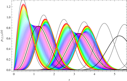
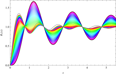
Figure 1: First four eigenvalue distributions $p_{1}(s),\ldots,p_{4}(s)$ (left) for $0.04\leq\rho\leq 0.70$ (step 0.01, purple to red) and the microscopic spectral density $R_{1}(x)$ (right) for $0.01\leq\rho\leq 1.00$ (step 0.01, purple to red) for the chGSE (black) to chGUE (gray) crossover, at $\nu=0$.

For comparison, the spectral densities that comprise the former, $R_{1}(x)=\sum_{k=1}^{\infty}p_{k}(x)=S(x,x)$ in Eq. (41), are plotted in Fig. 1 (right). The practical advantage of adopting individual eigenvalue distributions over $n$-level correlation functions (including $R_{1}(x)$) for fitting is clear from the figures: As the oscillation of the latter consists of overlapping multiple peaks, the characteristic shape of each peak is inevitably smeared, resulting in a rather structureless curve for which an accurate fit is difficult. On the other hand, the shape of the former is clearly distinguishable and is extremely sensitive to the $\rho$ parameter, because the ratio of the two $p_{k}(s)$ of the chGUE–chGSE crossover at different $\rho$ grows as $\exp(\mathrm{const.}s^{2})$ for large $s$. Therefore, the $p_{k}(s)$ are expected to admit very precise one-parameter fitting of data by the least-squares method (as will be shown in Tables 3–6 of Sect. 3).

2.7 Effective theory and low-energy constants

Now we shall relate the crossover random matrix ensemble to the nonlinear $\sigma$ models originating from gauge theory. In continuum, QCD-like theories with $N_{F}$ flavors of quarks in a real representation have pseudoreal Dirac operators, as does our case of SU(2) lattice gauge theory with fundamental staggered fermions (Eq. (69) in Sect. 3). The low-energy effective Lagrangian of these theories is universally determined by the spontaneous breaking of the Pauli–Gürsey extended flavor group $\mathrm{SU}(2N_{F})$ down to its vector subgroup $\mathrm{SO}(N_{F})$ and takes the form

$$\mathcal{L}_{\rm eff}(Q)=\frac{1}{2}F^{2}\,{\rm tr}\,\partial_{\nu}Q^{\dagger}\partial_{\nu}Q-\frac{1}{2}\Sigma m\,{\rm Re}\,{\rm tr}\,\hat{M}Q$$ (63)

in the leading order of the $p$-expansion. Here $Q(x)$ is a symmetric SU($2N_{F}$) matrix-valued Nambu–Goldstone field (called a nonlinear $\sigma$ model of class AI), $m$ the degenerate quark mass, and $\hat{M}=\sigma_{1}\otimes\mathbb{I}_{N_{F}}$. It contains two phenomenological constants: $F$ the pseudo-scalar decay constant and $\Sigma=\left\langle\bar{\psi}\psi\right\rangle/N_{F}$ the chiral condensate (both measured in the chiral and zero-chemical potential limit $m,\mu\to 0$). The effect of introducing the quark number chemical potential $\mu$ to the fundamental theory is unambiguously incorporated in $\mathcal{L}_{\rm eff}$ through flavor covariantization in the symmetric rank-2 tensor representation KSTVZ00 ,

$$\partial_{\nu}Q\ \mapsto\ \nabla_{\nu}Q=\partial_{\nu}Q-i\mu\delta_{\nu 0}(\hat{B}Q+Q\hat{B}),$$ (64)

with $\hat{B}=\sigma_{3}\otimes\mathbb{I}_{N_{F}}$. If the theory is in a finite volume $V=L^{4}$ and the Thouless energy defined as $E_{c}\sim{F^{2}}/(\Sigma L^{2})$ is much larger than $m$ (called the $\varepsilon$-regime), the path integral is dominated by the zero mode only and takes the form

$$Z=\int dQ\,\exp\left(V\mu^{2}F^{2}\,{\rm tr}\,(\hat{B}Q^{\dagger}\hat{B}Q+\hat{B}\hat{B})+\frac{1}{2}V\Sigma m\,{\rm Re}\,{\rm tr}\,\hat{M}Q\right).$$ (65)

The above form (not the concrete symmetric space on which $Q$ takes values) of action is in fact common for all classes of nonlinear $\sigma$ models (in even or odd dimensions, with Dyson indices $\beta=1,2,4$) in which the global symmetry is broken by the chemical potential DN03 .

On the other hand, the characteristic polynomial $\left\langle\det(\lambda-H)^{N_{F}}\right\rangle$ of a random matrix $H$ (3) in the microscopic crossover scaling limit explained in Sect. 2.5 can be evaluated by exponentiating the determinant with $N_{F}$ flavors of Grassmannian vectors and using a standard technique of Hubbard–Stratonovich transformations (see, e.g., Ref. Efe97 ) for matrices $A$ and $B$. One can easily show that the outcome is the same nonlinear $\sigma$ model as Eq. (65) with parameters replaced by

$$VF^{2}\mu^{2}\to\frac{\pi^{2}}{2}\rho^{2},\ \ \ V\Sigma m\to i\pi x,$$ (66)

respectively. Note that the above identification can also be read off from the exponents in the quaternion kernel elements (41)–(43).

3 Dirac spectrum

In this section we shall fit the probability distributions analytically derived in the previous section to the Dirac operator spectra measured from two types of lattice gauge simulations: (a) SU(2) gauge theory with the imaginary chemical potential, and (b) SU(2) $\times$ U(1) gauge theory. In either case the pseudoreality of the staggered SU(2) Dirac operator is weakly violated by the U(1) field, which is applied as a fixed background HOV97 or dynamically fluctuating.

3.1 Simulation details

(a) $\mathrm{SU}(2)$ gauge theory with the imaginary chemical potential (ICP): The $\mathrm{SU}(2)$ variables on temporal links of a hypercubic lattice of size $V=L^{4}$ are multiplied by a constant phase:

$$\tilde{U}_{\nu}(x)={U}_{\nu}(x)\times\begin{cases}{\rm e}^{i2\pi\varphi}&(\nu=4,\ x_{4}=L-1)\\ 1&\text{(else)}\end{cases}.$$ (67)

The phase $2\pi\varphi$ can be regarded as the Aharonov–Bohm (AB) flux DM91 penetrating the temporal circle and is gauge-equivalent to the imaginary chemical potential $\mu=i\mu_{\mathrm{I}}=2\pi i\varphi/L$, i.e., a fixed U(1) background $B_{\nu}=(2\pi\varphi/L)\delta_{\nu,4}$. We chose antiperiodic/periodic boundary conditions in the temporal/spatial directions, respectively, and consider a small twisting along the temporal direction ($\varphi\ll 1$).

(b) $\mathrm{SU}(2)\times\mathrm{U}(1)$ gauge theory: Following Ref. BDHIY07 , non-compact $\mathrm{U}(1)$ link variables $B_{\nu}(x)$ are generated under the Coulomb gauge-fixing condition (with an additional constraint for the $B_{4}(x)$) and at the unit coupling constant, and are multiplied to $\mathrm{SU}(2)$ link variables $U_{\nu}(x)$,

$$\tilde{U}_{\nu}(x)=U_{\nu}(x)\,e^{ieB_{\nu}(x)},$$ (68)

with $e$ denoting the bare $\mathrm{U}(1)$ coupling constant. Fermions are quenched both for the SU(2) and U(1) gauge fields. For the pure SU(2) case $e=0$ (or $\varphi=0$), the staggered $\mathrm{SU}(2)$ Dirac operator in the fundamental representation

$$D_{x,y}=\sum_{\nu=1}^{4}(-1)^{\sum_{i=1}^{\nu-1}x_{i}}\left(\tilde{U}_{\nu}(x)\delta_{x,y+\hat{\nu}}-\tilde{U}^{\dagger}_{\nu}(x)\delta_{x,y-\hat{\nu}}\right)$$ (69)

is pseudoreal, i.e., satisfies

$$\mathcal{T}D\mathcal{T}^{-1}=D\ \ \text{with}\ \ \mathcal{T}^{2}=(Z\mathcal{C})^{2}=-\mathbb{I}$$ (70)

($\mathcal{C}$ denotes complex conjugation) for either choice of periodic or antiperiodic boundary condition in each direction, and we impose periodic boundary conditions in all four directions and consider the $\mathrm{U}(1)$ part as a small perturbation (i.e., $e\ll 1$).

As the presence of the AB flux $\varphi$ or the $\mathrm{U}(1)$ coupling $e$ breaks the pseudoreality (70), they parametrize antiunitary symmetry breaking in Dirac operators and are anticipated to be the lattice gauge theory counterpart of the crossover parameter $\rho$ in random matrix ensemble interpolating chGSE and chGUE. We note that while the effect of the ICP $\mu_{\mathrm{I}}$ on the low-energy effective Lagrangian is completely dictated on the symmetry ground SV05 ; MT05 and is related to the pseudo-scalar decay constant $F$ as for the real chemical potential KSTVZ00 , the effect of $e$ cannot be directly related to $F$, because integrating over the dynamical U(1) gauge field in the effective Lagrangian would lead to nonlocal self-couplings of pseudo-scalar mesons.

3.1.1 Simulation setup

We measured low-lying spectra of the naïve staggered Dirac operator (69) on small lattices of volume $V=4^{4}$ and $6^{4}$. In order to examine the validity of our method for the strong-coupling to the near-continuum scaling regions, we chose the bare $\mathrm{SU}(2)$ gauge coupling constant $\beta=4/g^{2}$ from the range $\beta=0,0.25,\ldots,1.75$ (step $0.25$) on $V=4^{4}$ and $\beta=0,0.25,\ldots,2.0$ (step $0.25$), $2.1$ on $V=6^{4}$. The simplest algorithm is employed in generating SU(2) gauge configurations: unimproved plaquette action and the $10$-hit heat-bath update combined with over-relaxation. The antiunitary symmetry violation parameters are set to be: (a) $\varphi=0.01,\ldots,0.06$ (step 0.01) on $V=4^{4}$ and $\varphi=0.01,\ldots,0.05$ (step 0.005) on $V=6^{4}$, and (b) $e=0.002,\ldots,0.006$ (step $0.001$), 0.008, 0.0010 on $V=4^{4}$ and $e=0.0004,\ldots,0.0016$ (step $0.0002$), 0.0020, 0.0024, 0.0028 on $V=6^{4}$. $N_{\text{conf}}=40000$ (10000) configurations are generated and diagonalized on $V=4^{4}$ $(6^{4})$ for each set of parameters $(\beta,\varphi)$ or $(\beta,e)$.

3.1.2 Fitting Dirac spectra

Our procedure of fitting the Dirac spectra to the individual eigenvalue distributions of the crossover chiral random matrices consists of the following two steps:

1. Determination of the mean level spacing ${\varDelta}$ at the origin.   In order to determine the physical scale of Dirac eigenvalues upon which the effects of perturbations are to be evaluated, we measure for $N_{\text{conf}}$ independent configurations four low-lying nondegenerate eigenvalues $\lambda_{2i-1}=\lambda_{2i}\ (i=1,\ldots,4)$ of the pure SU(2) Dirac operator (due to its quaternionic nature, all eigenvalues are doubly degenerate).

   For each $i$, the mean level spacing $\varDelta_{i}$ at the spectral origin is determined by best-fitting the histogram of the unfolded Dirac eigenvalue $\lambda_{2i}/\varDelta_{i}$ to the normalized individual eigenvalue distribution $p_{i}(s)$ of chGSE so that $\chi^{2}/$d.o.f. is minimized by varying $\varDelta_{i}$. In doing so, we discard the left tail $[0,s_{\mathrm{min}}]$ and the right tail $[s_{\mathrm{max}},\infty)$ of the probability distribution $p_{i}(s)$ for which $\int_{0}^{s_{\mathrm{min}}}ds\,p_{i}(s)=\int_{s_{\mathrm{max}}}^{\infty}ds\,p_{i}(s)\simeq 10^{-3}$, and split the mid-range into $B$ bins of fixed widths $\delta s=0.1$, $[s_{\mathrm{min}},s_{\mathrm{max}}]=I_{1}\cup\cdots\cup I_{B}$. Then we define $\chi^{2}$ from the measured frequency $F_{b}=\#\{\lambda_{2i}\in I_{b}\}$ and its analytic prediction $f_{b}=N_{\text{conf}}\int_{I_{b}}ds\,p_{i}(s)$ by $\chi^{2}=\sum_{b=1}^{B}(F_{b}-f_{b})^{2}/f_{b}.$ The statistical error $\delta\varDelta_{i}$ is estimated as a deviation from the optimal $\varDelta_{i}$ at which $\chi^{2}/$d.o.f. increases by unity. The combined value of the mean level spacing at the origin $\bar{\varDelta}$ is obtained as the weighted average of $(\varDelta_{i},\delta\varDelta_{i}),\ i=1,\ldots,4$. We have confirmed that these four data are always mutually consistent, so that their combination helps to improve the statistical error in $\bar{\varDelta}$ as compared to the previous method of using the smallest eigenvalue only Nis12-1 ; Nis12-2 .

2. Determination of the crossover parameter $\rho$.   Next we switch on the U(1) perturbation (a) or (b) and measure the Dirac spectra $\{\lambda_{k}\}$ for $N_{\text{conf}}=\mathcal{O}(10^{4})$ independent configurations. The effect of such perturbations on $\varDelta$ (i.e., the chiral condensate) is negligible in the lowest order in the $\varepsilon$-expansion that we are working on. U(1) perturbations split once-Kramers-degenerate pairs of eigenvalues, $\lambda_{2i-1}<\lambda_{2i}$. We take the first two pairs of Dirac eigenvalues $(\lambda_{2i-1},\lambda_{2i}),i=1,2$, and define the unfolded eigenvalues as $(s_{2i-1},s_{2i})=(\lambda_{2i-1}/\varDelta_{i},\lambda_{2i}/\varDelta_{i}$). Then by using the same strategy as in Step (i), their histograms $P_{k}(s_{k})$ are fitted to the analytic results $p_{k}(s)$ (49), (57) of the crossover random matrices, with the crossover parameter $\rho_{k}$ being varied. The statistical error $\delta\rho_{k}$ of the crossover parameter is again estimated as a deviation from the optimal $\rho_{k}$ at which $\chi^{2}/\mathrm{d.o.f.}$ increases by unity.

   The crossover parameter $\bar{\rho}$ corresponding to a particular choice of $\varphi$ or $e$ is eventually determined as the weighted average of $(\rho_{k},\delta\rho_{k}),\ k=1,\ldots,4$. The advantage of using both once-degenerate eigenvalue pairs (over using, e.g., three low-lying eigenvalues) is now evident: Histograms of $s_{2i-1}$ and $s_{2i}$ always shift in the opposite directions under the Kramers-breaking perturbation, so that the effect of small errors in the determination of the overall scale $\varDelta_{i}$ in Step (i) (which shifts both histograms in the same direction) is expected to be canceled in the final value of $\bar{\rho}$ obtained by combining $\rho_{2i-1}$ and $\rho_{2i}$.

3.1.3 Low-energy constants

Due to the correspondence (66), two low-energy constants contained in the chiral Lagrangian, the chiral condensate $\Sigma$ and the pseudo-scalar decay constant $F$, are directly related to $\varDelta$ and $\rho$ measured in Steps (i) and (ii), the former by the Banks–Casher relation

$$\Sigma=\frac{\pi}{\varDelta V};$$ (71)

the latter for (a) the SU(2)+ICP model by

$$F^{2}=\frac{\pi^{2}}{2V}\left(\frac{{\rho}}{\mu_{\mathrm{I}}}\right)^{2}=\frac{\pi^{2}}{2V}\left(\frac{{\rho}}{2\pi\varphi/L}\right)^{2},$$ (72)

and for (b) the SU(2)$\times$U(1) model by

$$\frac{F^{2}\mu_{\mathrm{I}}^{2}}{e^{2}}=\frac{\pi^{2}}{2V}\left(\frac{\rho}{e}\right)^{2}.$$ (73)

Note that the combination “$F^{2}\mu_{\mathrm{I}}^{2}$” in the LHS of Eq. (73) is to be regarded as a single coefficient of the $-{\rm tr}\hat{B}Q^{\dagger}\hat{B}Q$ term in the chiral Lagrangian (65). As this quantity should be proportional to $e^{2}$, our aim here is to determine the unknown proportionality constant set by the dynamics. Thus we shall check, for each $\beta$ in either case of (a) or (b), the stability of the ratio $R(\varphi)=\rho/\varphi$ or $R(e)=\rho/e$ as $\varphi$ or $e$ is varied, and determine its mean value as a weighted average of $\{R(\varphi),\delta R(\varphi)\}$ or $\{R(e),\delta R(e)\}$.

3.2 Simulation results

3.2.1 Fitting Dirac spectra

In Tables 2 and 2 we exhibit optimal values of the mean level spacings $\varDelta_{i}$ of SU(2) Dirac spectra (a) under the antiperiodic boundary condition on the temporal direction (to be used for $\mathrm{SU}(2)+$ICP), and (b) under the periodic boundary conditions on all directions (to be used for $\mathrm{SU}(2)\times\mathrm{U}(1)$), respectively. At each $\beta$, we adopt only the $\varDelta_{i}$ that pass the $\chi^{2}$ test of the fitting: $\chi^{2}/\text{d.o.f.}<2.0$. In Fig. 2 (top) we exhibit sample plots of histograms of the four smallest nondegenerate Dirac eigenvalues $P_{i}(\lambda_{i})$ versus the corresponding individual eigenvalue distributions $p_{i}(s)$ of chGSE, each being optimally rescaled by $\varDelta_{i}$.

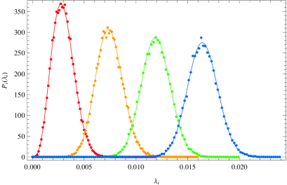
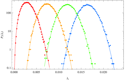
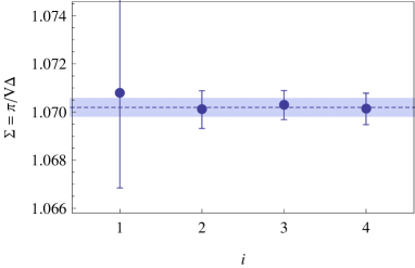
Figure 2: (Top) Linear and logarithmic plots of histograms of the four smallest nondegenerate Dirac eigenvalues $P_{i}(\lambda_{i})\ (i=1,\ldots,4)$ (red to blue) of pure SU(2) gauge theory at $\beta=1.0$, on $V=6^{4}$ and $N_{\mathrm{conf}}=30000$, and individual eigenvalue distributions $p_{i}(s)$ of chGSE, each being optimally rescaled by a constant $\varDelta_{i}$. (Bottom) Values of chiral condensate $\Sigma=\pi/(V\varDelta_{i})$ (circles), their weighted average (horizontal line), and the combined error (strip).

The mutual consistency of such $\varDelta_{i}$ observed in Fig. 2 (bottom) justifies the use of the weighted average, listed in the seventh columns in Tables 2 and 2. This sample figure illustrates that the error in $\varDelta_{1}$ (i.e., in $\Sigma$), which is relatively larger than that in the other three $\varDelta_{i}$, is considerably improved by a factor of 5–10 and is down to $\mathcal{O}(10^{-4})$ by the use of the weighted average of the four. Note that histograms at $\beta=1.75$ on $V=4^{4}$ and at $\beta=2.1$ on $V=6^{4}$ (marked by $*$ in Tables 2 and 2) failed to be fitted into the chGSE predictions in the above criterion as $\chi^{2}/\text{d.o.f.}$ exceeds 3. Thus we chose to relax it by cutting off the tails of the distributions for which $p_{1}(s)<0.2$ from fitting, which leads safely to $\chi^{2}/\text{d.o.f.}<2.0$.

Table 1: Mean level spacings of the pure $\mathrm{SU}(2)$ Dirac spectrum on $V=4^{4}$ and $6^{4}$ with the antiperiodic boundary condition on the temporal direction, in units of $10^{-2}a^{-1}$.

$V$	$\beta$	$\varDelta_{1}$	$\varDelta_{2}$	$\varDelta_{3}$	$\varDelta_{4}$	$\bar{\varDelta}$	$\chi^{2}/\text{d.o.f.}$
$4^{4}$	0	0.929(2)	0.931 5(7)	0.930 9(5)	0.931 3(4)	0.931 1(3)	0.99–1.00
	0.25	0.969(2)	0.970 8(9)	0.970 9(6)	0.970 3(4)	0.970 5(3)	0.85–1.00
	0.5	1.019(2)	1.019 0(9)	1.018 0(6)	1.017 5(4)	1.017 9(3)	0.74–1.02
	0.75	1.073(2)	1.073 5(8)	1.074 9(6)	1.075 6(5)	1.075 0(3)	1.01–1.36
	1.0	1.151(2)	1.150 0(9)	1.150 4(7)	–	1.150 3(5)	0.68–1.47
	1.25	1.255(2)	1.254(1)	–	–	1.254 4(9)	0.81–1.46
	1.5	1.408(3)	–	–	–	1.408(3)	0.73
	1.75∗	1.705(4)	–	–	–	1.705(4)	0.91
$6^{4}$	0	0.185 4(7)	0.185 2(3)	0.185 0(2)	0.185 2(2)	0.185 2(1)	0.92–1.02
	0.25	0.191 2(7)	0.192 6(3)	0.193 1(2)	0.192 7(2)	0.192 8(1)	0.98–1.20
	0.5	0.203 0(8)	0.202 7(4)	0.202 0(2)	0.202 3(2)	0.202 3(1)	0.95–0.99
	0.75	0.213 5(7)	0.213 3(2)	0.214 3(2)	0.213 5(2)	0.213 7(1)	0.85–1.01
	1.0	0.229 3(8)	0.227 7(4)	0.227 9(3)	0.227 8(2)	0.227 8(1)	0.93–1.00
	1.25	0.247 5(9)	0.248 0(4)	0.247 9(3)	0.248 1(2)	0.248 0(2)	0.63–0.99
	1.5	0.279 5(9)	0.278 7(5)	0.278 3(3)	0.277 9(2)	0.278 2(2)	0.96–1.00
	1.75	0.334(1)	0.333 1(6)	0.332 9(4)	–	0.333 0(3)	0.73–1.00
	2.0	0.482(2)	–	–	–	0.482(2)	1.12
	2.1∗	0.640(2)	–	–	–	0.640(2)	1.49

Table 2: Mean level spacings of the pure $\mathrm{SU}(2)$ Dirac spectrum on $V=4^{4}$ and $6^{4}$ with periodic boundary conditions on all four directions, in units of $10^{-2}a^{-1}$.

$V$	$\beta$	$\varDelta_{1}$	$\varDelta_{2}$	$\varDelta_{3}$	$\varDelta_{4}$	$\bar{\varDelta}$	$\chi^{2}/\text{d.o.f.}$
$4^{4}$	0	0.932(2)	0.930 6(8)	0.931 1(5)	0.931 3(4)	0.931 1(3)	0.62–1.13
	0.25	0.972(2)	0.971 8(8)	0.970 8(6)	0.970 4(4)	0.970 8(3)	0.84–1.13
	0.5	1.020(2)	1.016 0(9)	1.016 2(6)	1.017 0(4)	1.016 7(3)	0.97–1.20
	0.75	1.080(2)	1.077 0(9)	1.077 4(6)	1.076 5(5)	1.076 9(3)	0.76–1.15
	1.0	1.153(2)	1.152(1)	1.152 5(7)	–	1.152 4(5)	1.00–1.14
	1.25	1.249(2)	1.253(1)	–	–	1.252 5(9)	0.99–1.00
	1.5	1.412(2)	–	–	–	1.412(2)	0.93
	1.75∗	1.698(3)	–	–	–	1.698(3)	1.35
$6^{4}$	0	0.186 5(6)	0.185 4(3)	0.185 3(2)	0.185 4(2)	0.185 4(1)	0.79–1.00
	0.25	0.192 8(7)	0.192 9(3)	0.192 8(2)	0.192 8(2)	0.192 8(1)	0.99–1.00
	0.5	0.202 4(8)	0.202 4(4)	0.202 0(2)	0.202 0(2)	0.202 1(1)	0.77–1.01
	0.75	0.214 6(8)	0.213 7(4)	0.213 8(2)	0.213 6(2)	0.213 7(1)	0.98–1.01
	1.0	0.228 6(8)	0.229 2(4)	0.228 5(3)	0.228 5(2)	0.228 6(1)	0.99–1.00
	1.25	0.248 1(9)	0.247 8(6)	0.248 4(3)	0.247 7(2)	0.248 0(2)	0.97–1.01
	1.5	0.277(1)	0.277 8(5)	0.278 3(3)	0.278 2(2)	0.278 1(2)	0.99–1.00
	1.75	0.333(1)	0.331 8(6)	0.333 1(4)	–	0.332 7(3)	0.96–1.24
	2.0	0.480(2)	–	–	–	0.480(2)	1.66
	2.1∗	0.639(3)	–	–	–	0.639(3)	0.99

Next we exhibit the optimal values of the crossover parameters $\rho_{k}(k=1,\ldots,4)$, determined by fitting individual Dirac eigenvalue histograms to the chGSE–chGUE predictions, (a) for the SU(2)+ICP model in Tables 3 and 4, and (b) for the SU(2)$\times$U(1) model in Tables 5 and 6. Again we adopted only the cases that passed the $\chi^{2}$ test with $\chi^{2}/\text{d.o.f.}<2.0$, and the exceptional treatment of cutting off the tails of the smallest eigenvalue distributions for which $p_{1}(s)<0.2$ from fitting is applied to $\beta=1.75$ on $V=4^{4}$ and $\beta=2.1$ on $V=6^{4}$ (marked by $*$ in Tables 3–6). Whenever the histogram of the unfolded eigenvalues $s_{2i-1}=s_{2i}$ of the pure SU(2) Dirac operator is well fitted into the chGSE prediction in our criterion, so is the corresponding pair $\{P_{2i-1}(s_{2i-1}),P_{2i}(s_{2i})\}$ of the perturbed Dirac operator to the chGSE–chGUE crossover prediction, as expected.

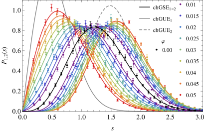
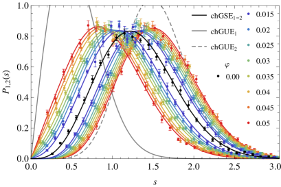
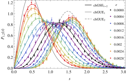
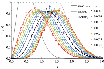
Figure 3: The first two Dirac eigenvalue distributions $P_{1,2}(s)$ of the SU(2)+ICP model (top) and SU(2)$\times$U(1) model (bottom) with increasing perturbations $\varphi$ and $e$, from black ($\varphi,e=0$) to purple (smallest $\varphi,e$) to red (largest $\varphi,e$), on $V=6^{4}$ and at $\beta=1.0$ (left) and at $\beta=2.0$ (right). Those of chGSE and chGUE are plotted in black and gray, respectively, and the best-fit curves of the chGSE–chGUE crossover are plotted in the same colors as the corresponding lattice data. The error bars of the histograms in Figs. 3–5 are estimated by the jackknife method.

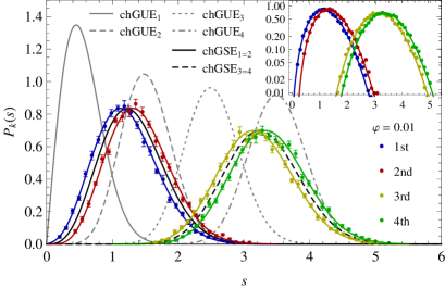
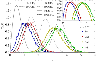
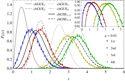
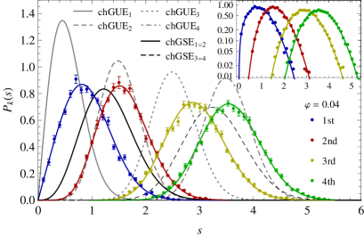
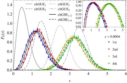
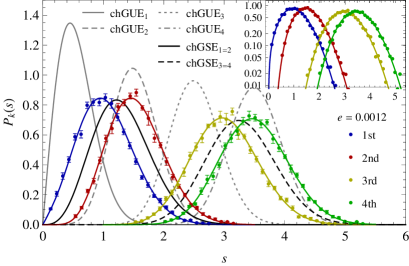
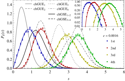
Figure 4: Linear and logarithmic (inset) plots of the first four Dirac eigenvalue distributions $P_{1,2,3,4}(s)$ (blue, red, yellow, green) of the SU(2)+ICP model on $V=6^{4}$ and at $\beta=1.75$, and best-fit curves of the chGSE–chGUE crossover. Top left: $\varphi=0.01$, top right: $\varphi=0.02$, bottom left: $\varphi=0.03$, bottom right: $\varphi=0.04$.

Figure 5: Linear and logarithmic (inset) plots of the first four Dirac eigenvalue distributions $P_{1,2,3,4}(s)$ (blue, red, yellow, green) of the SU(2)$\times$U(1) model on $V=6^{4}$ and at $\beta=1.75$, and best-fit curves of the chGSE–chGUE crossover. Top left: $e=0.0004$, top right: $e=0.0008$, bottom left: $e=0.0012$ and bottom right: $e=0.0016$.

Figure 3 shows samples of the histograms $\{P_{1}(s_{1}),P_{2}(s_{2})\}$ of the perturbed Dirac operator eigenvalues and best-fit distributions of the chGSE–chGUE crossover. As the perturbation $\varphi$ or $e$ is increased, the eigenvalue distributions are clearly seen to follow the random matrix curves. They respond more rapidly to the perturbation for smaller $\beta$ (left panels) than for larger $\beta$ (right panels), indicating that $F$ is a decreasing function of $\beta$. For the sake of graphical visibility, we also exhibit samples of histograms of $\{P_{1}(s_{1}),\ldots,P_{4}(s_{4})\}$ and best-fit distributions of the chGSE–chGUE crossover, at fixed $\beta=1.75$ and with increasing perturbations $\varphi$ (Fig. 5) and $e$ (Fig. 5), respectively.

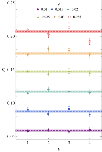
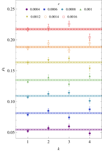
Figure 6: Crossover parameters $\rho_{1,2,3,4}$ determined from $P_{1,2,3,4}(s)$. Their weighted averages and combined errors are shown in horizontal lines and strips. Left: SU(2)+ICP model with $\varphi=0.01$–0.035 (purple to red). Right: SU(2)$\times$U(1) model with $e=0.0004$–0.0016 (purple to red). Both are at $\beta=1.75$ and on $V=6^{4}$.

Figure 6 illustrates the crossover parameters $\rho_{k}$ determined from $P_{k}(s_{k})$ for the SU(2)+ICP model and for the SU(2)$\times$U(1) model at $\beta=1.75$ and $V=6^{4}$, at each value of perturbation $\varphi$ or $e$. We notice that $\rho_{1}$ and $\rho_{2}$ ($\rho_{3}$ and $\rho_{4}$) have a tendency to counter-move across the weighted average of the four, as anticipated in Sect. 3.1. Combined use of $P_{2i-1}(s_{2i-1})$ and $P_{2i}(s_{2i})$ is indeed seen to reduce the errors of the best-fit parameters $\bar{\rho}$ in both panels.

Table 3: Crossover parameters $\rho$ for the SU(2)+ICP model on $V=4^{4}$.

		$\varphi$
$\beta$	$\rho$	0.01	0.02	0.03	0.04	0.05	0.06	$\chi^{2}/\text{d.o.f.}$
0	$\rho_{1}$	0.061(1)	0.122(1)	0.183(1)	0.244(2)	–	–	0.68–1.06
	$\rho_{2}$	0.061(2)	0.121(2)	0.183(2)	0.238(3)	–	–	0.95–1.71
	$\rho_{3}$	0.060(2)	0.118(2)	0.181(2)	0.243(2)	–	–	0.50.–0.69
	$\rho_{4}$	0.062(2)	0.125(2)	0.184(2)	0.245(3)	–	–	0.64–1.19
	$\bar{\rho}$	0.061 2(8)	0.121 4(9)	0.183(1)	0.243(1)	–	–	–
0.25	$\rho_{1}$	0.060(1)	0.117(1)	0.176(1)	0.234(2)	0.291(2)	–	0.65–1.21
	$\rho_{2}$	0.057(2)	0.118(2)	0.174(2)	0.234(3)	0.296(4)	–	0.63–1.22
	$\rho_{3}$	0.062(2)	0.117(2)	0.176(2)	0.235(2)	0.291(3)	–	0.80–1.49
	$\rho_{4}$	0.056(2)	0.116(2)	0.174(2)	0.231(3)	0.298(4)	–	0.76–1.30
	$\bar{\rho}$	0.058 6(8)	0.116 9(9)	0.175 3(9)	0.234(1)	0.292(1)	–	–
0.5	$\rho_{1}$	0.056(1)	0.108(1)	0.168(1)	0.224(2)	0.279(2)	–	0.57–1.56
	$\rho_{2}$	0.056(2)	0.117(2)	0.167(2)	0.227(3)	0.282(4)	–	0.35–1.33
	$\rho_{3}$	0.056(2)	0.111(2)	0.165(2)	0.228(2)	0.279(2)	–	0.64–1.25
	$\rho_{4}$	0.057(2)	0.112(2)	0.171(2)	0.217(3)	0.277(4)	–	0.82–1.34
	$\bar{\rho}$	0.056 1(8)	0.111 3(9)	0.167 7(9)	0.224(1)	0.279(1)	–	–
0.75	$\rho_{1}$	0.055(1)	0.108(1)	0.162(1)	0.216(1)	0.270(2)	–	0.63–0.90
	$\rho_{2}$	0.053(2)	0.106(2)	0.159(2)	0.213(3)	0.266(4)	–	0.76–1.23
	$\rho_{3}$	0.056(2)	0.110(2)	0.164(2)	0.218(2)	0.271(2)	–	0.78–1.39
	$\rho_{4}$	0.051(2)	0.104(2)	0.158(2)	0.210(3)	0.262(3)	–	0.98–1.18
	$\bar{\rho}$	0.053 8(8)	0.107 3(9)	0.161 0(9)	0.215(1)	0.269(1)	–	–
1.0	$\rho_{1}$	0.052(1)	0.102(1)	0.153(1)	0.203(1)	0.254(2)	–	0.78–1.05
	$\rho_{2}$	0.050(2)	0.101(2)	0.151(2)	0.201(2)	0.251(3)	–	0.60–1.16
	$\rho_{3}$	0.050(2)	0.101(2)	0.151(2)	0.202(2)	0.252(2)	–	0.78–1.39
	$\rho_{4}$	0.051(2)	0.102(2)	0.153(2)	0.204(3)	0.253(3)	–	0.90–1.23
	$\bar{\rho}$	0.050 8(8)	0.101 5(9)	0.152 2(9)	0.203(1)	0.253(1)	–	–
1.25	$\rho_{1}$	0.048(1)	0.096(1)	0.143(1)	0.190(1)	0.238(2)	0.285(2)	0.88–1.23
	$\rho_{2}$	0.047(2)	0.095(2)	0.142(2)	0.189(2)	0.236(3)	0.283(4)	0.70–1.14
	$\rho_{3}$	–	–	–	–	–	–	–
	$\rho_{4}$	–	–	–	–	–	–	–
	$\bar{\rho}$	0.048(1)	0.095(1)	0.143(9)	0.190(1)	0.237(1)	0.285(2)	–
1.5	$\rho_{1}$	–	0.087(1)	0.130(1)	0.174(1)	0.217(2)	0.261(2)	0.69–0.94
	$\rho_{2}$	–	0.086(2)	0.129(2)	0.172(2)	0.214(3)	0.254(3)	0.62–1.03
	$\rho_{3}$	–	–	–	–	–	–	–
	$\rho_{4}$	–	–	–	–	–	–	–
	$\bar{\rho}$	–	0.087(1)	0.130(1)	0.173(1)	0.216(1)	0.259(1)	–
1.75∗	$\rho_{1}$	–	0.075(2)	0.113(2)	0.150(2)	0.188(2)	0.226(2)	0.88–1.99
	$\rho_{2}$	–	0.074(2)	0.110(2)	0.147(3)	0.180(3)	0.216(4)	0.56–1.30
	$\rho_{3}$	–	–	–	–	–	–	–
	$\rho_{4}$	–	–	–	–	–	–	–
	$\bar{\rho}$	–	0.075(1)	0.112(2)	0.149(2)	0.186(2)	0.224(2)	–

Table 4: Crossover parameters $\rho$ for the SU(2)+ICP model on $V=6^{4}$.

		$\varphi$
$\beta$	$\rho$	0.01	0.015	0.02	0.025	0.03	0.035	0.04	0.045	0.05	$\chi^{2}/\text{d.o.f.}$
0	$\rho_{1}$	0.093(3)	0.135(3)	0.178(3)	0.228(3)	–	–	–	–	–	0.54-1.18
	$\rho_{2}$	0.089(3)	0.138(4)	0.187(5)	0.228(6)	–	–	–	–	–	0.47–1.40
	$\rho_{3}$	0.083(4)	0.135(4)	0.173(4)	0.223(4)	–	–	–	–	–	0.56–1.30
	$\rho_{4}$	0.099(4)	0.138(4)	0.191(5)	0.236(6)	–	–	–	–	–	0.76–1.09
	$\bar{\rho}$	0.091(2)	0.136(2)	0.180(2)	0.228(2)	–	–	–	–	–	–
0.25	$\rho_{1}$	0.088(3)	0.135(3)	0.177(3)	0.223(3)	–	–	–	–	–	0.87–1.32
	$\rho_{2}$	0.087(3)	0.130(4)	0.171(4)	0.215(5)	–	–	–	–	–	0.51–1.37
	$\rho_{3}$	0.090(4)	0.133(4)	0.179(4)	0.218(4)	–	–	–	–	–	0.66–1.05
	$\rho_{4}$	0.087(4)	0.132(4)	0.169(4)	0.229(6)	–	–	–	–	–	0.76–1.19
	$\bar{\rho}$	0.088(2)	0.133(2)	0.175(2)	0.221(2)	–	–	–	–	–	–
0.5	$\rho_{1}$	0.083(3)	0.119(3)	0.168(3)	0.217(3)	–	–	–	–	–	0.96–1.25
	$\rho_{2}$	0.085(3)	0.135(4)	0.170(4)	0.201(5)	–	–	–	–	–	0.60–0.94
	$\rho_{3}$	0.083(4)	0.123(4)	0.166(4)	0.222(4)	–	–	–	–	–	0.77–1.32
	$\rho_{4}$	0.086(4)	0.130(4)	0.173(5)	0.200(5)	–	–	–	–	–	0.48–1.23
	$\bar{\rho}$	0.084(2)	0.125(2)	0.169(2)	0.213(2)	–	–	–	–	–	–
0.75	$\rho_{1}$	0.082(3)	0.123(3)	0.157(3)	0.202(3)	0.240(3)	–	–	–	–	0.70–1.47
	$\rho_{2}$	0.077(3)	0.119(4)	0.171(4)	0.205(5)	0.246(6)	–	–	–	–	0.46–1.12
	$\rho_{3}$	0.087(4)	0.124(4)	0.163(4)	0.207(4)	0.241(4)	–	–	–	–	0.60–1.14
	$\rho_{4}$	0.076(4)	0.116(4)	0.159(4)	0.200(5)	0.244(6)	–	–	–	–	0.80–1.33
	$\bar{\rho}$	0.081(2)	0.121(2)	0.161(2)	0.203(2)	0.242(2)	–	–	–	–	–
1.0	$\rho_{1}$	0.076(3)	0.111(3)	0.153(3)	0.188(3)	0.233(3)	–	–	–	–	0.49–0.97
	$\rho_{2}$	0.080(3)	0.117(4)	0.157(4)	0.197(5)	0.228(6)	–	–	–	–	0.71–1.27
	$\rho_{3}$	0.078(4)	0.108(4)	0.146(4)	0.186(4)	0.227(4)	–	–	–	–	0.75–1.38
	$\rho_{4}$	0.078(4)	0.125(4)	0.165(5)	0.199(5)	0.233(6)	–	–	–	–	0.70–1.13
	$\bar{\rho}$	0.078(2)	0.114(2)	0.154(2)	0.191(2)	0.231(2)	–	–	–	–	–
1.25	$\rho_{1}$	0.074(3)	0.107(3)	0.146(3)	0.180(3)	0.213(3)	–	–	–	–	0.54–1.31
	$\rho_{2}$	0.073(3)	0.113(4)	0.144(4)	0.180(5)	0.219(5)	–	–	–	–	0.67–1.05
	$\rho_{3}$	0.071(4)	0.106(4)	0.152(4)	0.181(4)	0.214(4)	–	–	–	–	0.84–0.98
	$\rho_{4}$	0.074(4)	0.111(4)	0.138(4)	0.179(5)	0.222(5)	–	–	–	–	0.66–1.24
	$\bar{\rho}$	0.073(2)	0.109(2)	0.145(2)	0.180(2)	0.216(2)	–	–	–	–	–
1.5	$\rho_{1}$	0.068(3)	0.099(3)	0.136(3)	0.169(3)	0.196(3)	0.230(3)	–	–	–	0.6–0.89
	$\rho_{2}$	0.067(3)	0.104(4)	0.132(4)	0.158(4)	0.206(5)	0.240(6)	–	–	–	0.60–1.02
	$\rho_{3}$	0.069(4)	0.106(4)	0.141(4)	0.172(4)	0.201(4)	0.232(4)	–	–	–	0.80–1.17
	$\rho_{4}$	0.063(4)	0.094(4)	0.128(4)	0.157(4)	0.200(5)	0.231(6)	–	–	–	0.84–1.32
	$\bar{\rho}$	0.067(2)	0.100(2)	0.135(2)	0.166(2)	0.199(2)	0.232(2)	–	–	–	–
1.75	$\rho_{1}$	0.058(3)	0.090(3)	0.115(3)	0.148(3)	0.172(3)	0.209(3)	–	–	–	0.67–1.21
	$\rho_{2}$	0.060(3)	0.084(3)	0.121(4)	0.144(4)	0.181(5)	0.203(5)	–	–	–	0.67–1.60
	$\rho_{3}$	0.057(4)	0.091(4)	0.117(4)	0.148(4)	0.178(4)	0.216(4)	–	–	–	0.76–1.54
	$\rho_{4}$	0.060(4)	0.083(4)	0.116(4)	0.145(4)	0.172(5)	0.192(5)	–	–	–	0.77–1.68
	$\bar{\rho}$	0.059(2)	0.087(2)	0.117(2)	0.147(2)	0.175(2)	0.207(2)	–	–	–	–
2.0	$\rho_{1}$	–	0.072(3)	0.095(3)	0.117(3)	0.140(3)	0.163(3)	0.185(3)	0.207(3)	0.230(3)	0.94–1.48
	$\rho_{2}$	–	0.063(3)	0.085(3)	0.108(4)	0.131(4)	0.152(4)	0.173(4)	0.194(5)	0.214(5)	0.90–1.37
	$\rho_{3}$	–	–	–	–	–	–	–	–	–	–
	$\rho_{4}$	–	–	–	–	–	–	–	–	–	–
	$\bar{\rho}$	–	0.068(2)	0.091(2)	0.114(2)	0.137(2)	0.159(2)	0.181(2)	0.204(3)	0.226(3)	–
2.1∗	$\rho_{1}$	–	–	0.079(4)	–	0.114(4)	0.133(4)	0.151(4)	0.170(4)	0.189(4)	1.55–1.90
	$\rho_{2}$	–	–	0.064(5)	-	0.101(5)	0.119(5)	0.137(5)	0.150(6)	0.167(6)	1.42–1.94
	$\rho_{3}$	–	–	–	–	–	–	–	–	–	–
	$\rho_{4}$	–	–	–	–	–	–	–	–	–	–
	$\bar{\rho}$	–	–	0.073(3)	–	0.109(3)	0.128(3)	0.147(3)	0.165(3)	0.183(3)	–

Table 5: Crossover parameters $\rho$ for the SU(2)$\times$U(1) model on $V=4^{4}$.

		$e$
$\beta$	$\rho$	0.002	0.003	0.004	0.005	0.006	0.008	0.010	$\chi^{2}/\text{d.o.f.}$
0	$\rho_{1}$	0.093(1)	0.136(1)	0.186(1)	0.232(2)	0.276(2)	–	–	0.62–1.52
	$\rho_{2}$	0.905(2)	0.142(2)	0.181(2)	0.225(3)	0.277(4)	–	–	0.73–1.38
	$\rho_{3}$	0.089(2)	0.136(2)	0.183(2)	0.231(2)	0.273(2)	–	–	0.82–1.20
	$\rho_{4}$	0.094(2)	0.139(2)	0.187(2)	0.230(3)	0.280(4)	–	–	0.81–1.08
	$\bar{\rho}$	0.091 8(8)	0.137 8(9)	0.184(1)	0.230(1)	0.276(1)	–	–	–
0.25	$\rho_{1}$	0.088(1)	0.136(1)	0.176(1)	0.225(2)	0.265(2)	–	–	0.48–1.14
	$\rho_{2}$	0.088(2)	0.128(2)	0.177(2)	0.216(3)	0.264(3)	–	–	0.76–1.75
	$\rho_{3}$	0.087(2)	0.137(2)	0.175(2)	0.226(2)	0.262(2)	–	–	0.55–1.04
	$\rho_{4}$	0.088(2)	0.128(2)	0.176(2)	0.214(3)	0.261(3)	–	–	0.75–1.53
	$\bar{\rho}$	0.088 0(8)	0.133 1(9)	0.176 0(9)	0.222(1)	0.264(1)	–	–	–
0.5	$\rho_{1}$	0.083(1)	0.126(1)	0.167(1)	0.210(2)	0.251(2)	–	–	0.50–0.99
	$\rho_{2}$	0.086(2)	0.128(2)	0.170(2)	0.212(3)	0.256(3)	–	–	0.53–0.94
	$\rho_{3}$	0.086(2)	0.121(2)	0.170(2)	0.206(2)	0.255(2)	–	–	0.79–1.34
	$\rho_{4}$	0.082(2)	0.133(2)	0.166(2)	0.218(3)	0.248(3)	–	–	0.38–1.34
	$\bar{\rho}$	0.084 0(8)	0.126 2(9)	0.168 2(9)	0.210(1)	0.252(1)	–	–	–
0.75	$\rho_{1}$	0.078(1)	0.118(1)	0.159(1)	0.199(1)	0.239(2)	–	–	0.68–1.22
	$\rho_{2}$	0.082(2)	0.122(2)	0.163(2)	0.202(2)	0.244(3)	–	–	0.48–0.84
	$\rho_{3}$	0.081(2)	0.116(2)	0.161(2)	0.196(2)	0.242(2)	–	–	0.72–1.01
	$\rho_{4}$	0.080(2)	0.124(2)	0.159(2)	0.204(3)	0.237(3)	–	–	0.62–1.40
	$\bar{\rho}$	0.079 9(8)	0.119 8(9)	0.160 2(9)	0.200(1)	0.240(1)	–	–	–
1.0	$\rho_{1}$	0.075(1)	0.114(1)	0.150(1)	0.189(1)	0.225(2)	0.300(2)	–	0.75–1.27
	$\rho_{2}$	0.075(2)	0.111(2)	0.150(2)	0.184(2)	0.223(3)	0.296(4)	–	1.00–1.55
	$\rho_{3}$	0.076(2)	0.114(2)	0.151(2)	0.189(2)	0.226(2)	0.303(3)	–	0.94–1.62
	$\rho_{4}$	0.073(2)	0.111(2)	0.147(2)	0.183(2)	0.218(2)	0.283(4)	–	0.86–1.20
	$\bar{\rho}$	0.074 8(8)	0.112 6(9)	0.149 4(9)	0.187(1)	0.224(1)	0.298(1)	–	–
1.25	$\rho_{1}$	0.068(1)	0.103(1)	0.138(1)	0.172(1)	0.208(1)	0.278(2)	–	0.60–1.15
	$\rho_{2}$	0.069(2)	0.104(2)	0.138(2)	0.172(2)	0.206(3)	0.272(4)	–	0.53–0.95
	$\rho_{3}$	0.069(2)	0.107(2)	0.139(2)	0.177(2)	0.210(2)	0.281(2)	–	1.14–1.57
	$\rho_{4}$	0.069(2)	0.097(2)	0.134(2)	0.162(2)	0.201(3)	0.264(3)	–	1.32–1.65
	$\bar{\rho}$	0.068 8(8)	0.103 2(8)	0.137 7(9)	0.171 6(9)	0.207(1)	0.276(1)	–	–
1.5	$\rho_{1}$	0.063(1)	0.092(1)	0.125(1)	0.154(1)	0.187(1)	0.250(2)	0.313(2)	0.68–1.06
	$\rho_{2}$	0.060(2)	0.093(2)	0.121(2)	0.154(2)	0.180(2)	0.236(3)	0.286(4)	0.61–1.25
	$\rho_{3}$	–	–	–	–	–	–	–	–
	$\rho_{4}$	–	–	–	–	–	–	–	–
	$\bar{\rho}$	0.062(1)	0.092(1)	0.123(1)	0.154(1)	0.185(1)	0.246(1)	0.308(2)	–
1.75∗	$\rho_{1}$	0.054(2)	–	0.106(2)	–	0.158(2)	0.210(2)	0.263(2)	1.35–1.63
	$\rho_{2}$	0.049(2)	–	0.100(2)	–	0.148(2)	0.195(3)	0.236(3)	1.16–1.77
	$\rho_{3}$	–	–	–	–	–	–	–	–
	$\rho_{4}$	–	–	–	–	–	–	–	–
	$\bar{\rho}$	0.052(1)	–	0.103(1)	–	0.154(1)	0.206(1)	0.258(2)	–

Table 6: Crossover parameters $\rho$ for the SU(2)$\times$U(1) model on $V=6^{4}$.

		$e$
$\beta$	$\rho$	0.0004	0.0006	0.0008	0.0010	0.0012	0.0014	0.0016	0.0020	0.0024	0.0028	$\chi^{2}/\text{d.o.f.}$
0	$\rho_{1}$	0.090(3)	0.149(3)	0.192(3)	0.241(3)	–	–	–	–	–	–	0.72–1.03
	$\rho_{2}$	0.102(4)	0.134(4)	0.187(5)	0.232(6)	–	–	–	–	–	–	0.97–1.31
	$\rho_{3}$	0.098(4)	0.147(4)	0.196(4)	0.236(4)	–	–	–	–	–	–	0.67–1.45
	$\rho_{4}$	0.092(4)	0.138(4)	0.183(5)	0.240(6)	–	–	–	–	–	–	0.59–1.09
	$\bar{\rho}$	0.095(2)	0.143(2)	0.190(2)	0.238(2)	–	–	–	–	–	–	–
0.25	$\rho_{1}$	0.093(3)	0.134(3)	0.185(3)	0.225(3)	–	–	–	–	–	–	0.49–1.21
	$\rho_{2}$	0.089(3)	0.143(4)	0.180(5)	0.238(6)	–	–	–	–	–	–	0.97–1.41
	$\rho_{3}$	0.093(4)	0.132(4)	0.184(4)	0.223(4)	–	–	–	–	–	–	0.67–1.31
	$\rho_{4}$	0.090(4)	0.147(4)	0.180(5)	0.243(6)	–	–	–	–	–	–	1.01–1.51
	$\bar{\rho}$	0.092(2)	0.138(2)	0.183(2)	0.228(2)	–	–	–	–	–	–	–
0.5	$\rho_{1}$	0.090(3)	0.127(3)	0.177(3)	0.215(3)	–	–	–	–	–	–	0.73–1.19
	$\rho_{2}$	0.085(3)	0.140(4)	0.173(4)	0.230(6)	–	–	–	–	–	–	0.57–1.20
	$\rho_{3}$	0.085(4)	0.128(4)	0.173(4)	0.214(4)	–	–	–	–	–	–	0.64–1.10
	$\rho_{4}$	0.091(4)	0.135(4)	0.180(5)	0.222(5)	–	–	–	–	–	–	0.82–0.98
	$\bar{\rho}$	0.088(2)	0.131(2)	0.176(2)	0.218(2)	–	–	–	–	–	–	–
0.75	$\rho_{1}$	0.082(3)	0.124(3)	0.166(3)	0.206(3)	0.249(3)	–	–	–	–	–	0.77–0.96
	$\rho_{2}$	0.084(3)	0.128(4)	0.167(4)	0.213(5)	0.250(6)	–	–	–	–	–	0.74–0.79
	$\rho_{3}$	0.082(4)	0.123(4)	0.166(4)	0.205(4)	0.248(5)	–	–	–	–	–	0.84–1.02
	$\rho_{4}$	0.082(4)	0.129(4)	0.163(4)	0.214(5)	0.244(6)	–	–	–	–	–	0.94–1.12
	$\bar{\rho}$	0.082(2)	0.125(2)	0.166(2)	0.208(2)	0.248(2)	–	–	–	–	–	–
1.0	$\rho_{1}$	0.081(3)	0.116(3)	0.155(3)	0.193(3)	0.232(3)	–	–	–	–	–	1.02–1.36
	$\rho_{2}$	0.073(3)	0.117(4)	0.154(4)	0.194(5)	0.231(6)	–	–	–	–	–	0.75–1.01
	$\rho_{3}$	0.083(4)	0.113(4)	0.161(4)	0.191(4)	0.241(5)	–	–	–	–	–	0.36–1.45
	$\rho_{4}$	0.072(4)	0.119(4)	0.155(4)	0.196(5)	0.234(6)	–	–	–	–	–	0.75–1.09
	$\bar{\rho}$	0.078(2)	0.116(2)	0.156(2)	0.193(2)	0.234(2)	–	–	–	–	–	–
1.25	$\rho_{1}$	0.070(3)	0.108(3)	0.143(3)	0.178(3)	0.216(3)	–	–	–	–	–	0.70–1.13
	$\rho_{2}$	0.076(3)	0.110(4)	0.149(4)	0.182(5)	0.222(6)	–	–	–	–	–	0.76–0.95
	$\rho_{3}$	0.073(4)	0.111(4)	0.144(4)	0.184(4)	0.217(4)	–	–	–	–	–	0.87–1.23
	$\rho_{4}$	0.071(4)	0.108(4)	0.143(4)	0.179(5)	0.213(5)	–	–	–	–	–	0.48–0.94
	$\bar{\rho}$	0.072(2)	0.109(2)	0.144(2)	0.180(2)	0.217(2)	–	–	–	–	–	–
1.5	$\rho_{1}$	0.062(3)	0.095(3)	0.130(3)	0.160(3)	0.195(3)	–	–	–	–	–	0.77–1.33
	$\rho_{2}$	0.068(3)	0.098(3)	0.132(4)	0.165(4)	0.196(5)	–	–	–	–	–	0.68–1.26
	$\rho_{3}$	0.069(4)	0.100(4)	0.129(4)	0.164(4)	0.193(4)	–	–	–	–	–	0.78–1.25
	$\rho_{4}$	0.059(4)	0.094(4)	0.127(4)	0.157(4)	0.189(5)	–	–	–	–	–	0.96–0.99
	$\bar{\rho}$	0.064(2)	0.097(2)	0.130(2)	0.161(2)	0.194(2)	–	–	–	–	–	–
1.75	$\rho_{1}$	0.052(3)	0.079(3)	0.108(3)	0.133(3)	0.163(3)	0.187(3)	0.217(3)	–	–	–	0.93–1.24
	$\rho_{2}$	0.057(3)	0.085(3)	0.113(4)	0.140(4)	0.167(4)	0.194(5)	0.220(5)	–	–	–	0.87–1.20
	$\rho_{3}$	0.060(4)	0.075(4)	0.115(4)	0.129(4)	0.170(4)	0.183(4)	0.226(4)	–	–	–	0.66–1.22
	$\rho_{4}$	0.049(4)	0.088(4)	0.102(4)	0.141(4)	0.154(4)	0.195(5)	0.204(5)	–	–	–	0.46–1.09
	$\bar{\rho}$	0.055(2)	0.081(2)	0.109(2)	0.135(2)	0.163(2)	0.188(2)	0.217(2)	–	–	–	–
2.0	$\rho_{1}$	–	0.057(3)	0.080(3)	0.096(3)	0.118(3)	0.134(3)	0.156(3)	0.194(3)	0.234(3)	0.272(3)	0.95–1.44
	$\rho_{2}$	–	0.058(3)	0.073(3)	0.095(3)	0.110(4)	0.132(4)	0.147(4)	0.180(5)	0.215(5)	0.244(6)	0.90–1.94
	$\rho_{3}$	–	–	–	–	–	–	–	–	–	–	–
	$\rho_{4}$	–	–	–	–	–	–	–	–	–	–	–
	$\bar{\rho}$	–	0.57(2)	0.077(2)	0.096(2)	0.115(2)	0.133(2)	0.153(2)	0.190(2)	0.229(3)	0.266(3)	–
2.1∗	$\rho_{1}$	–	–	0.062(4)	–	0.091(4)	–	–	0.147(4)	0.176(4)	0.205(4)	1.03–1.56
	$\rho_{2}$	–	–	0.059(5)	–	0.087(5)	–	–	0.139(5)	0.162(6)	0.187(7)	1.29–1.76
	$\rho_{3}$	–	–	–	–	–	–	–	–	–	–	–
	$\rho_{4}$	–	–	–	–	–	–	–	–	–	–	–
	$\bar{\rho}$	–	–	0.061(3)	–	0.089(3)	–	–	0.144(3)	0.172(3)	0.201(3)	–

3.2.2 Low-energy constants

The chiral condensate $\Sigma$ is determined by Eq. (71) from $\bar{\varDelta}$ summarized in Tables 2 and 2. In Table 7 we list these values in the third column (SU(2)+ICP) and in the fifth column (SU(2)$\times$U(1)), at each $\beta$ and on $V=4^{4}$ and $6^{4}$ lattices. In addition, the values of the chiral condensate in the thermodynamic limit $V=\infty$, extrapolated from $V=4^{4}$ and $6^{4}$, are listed for the coupling range $0\leq\beta\leq 1.75$.

The pseudo-scalar decay constant $F$ in Eqs. (72) and (73) is essentially the proportionality constant between the perturbation strength $\mu_{\mathrm{I}}$ or $e$ and the crossover parameter $\rho$. In Fig. 7 we exhibit the ratios $\bar{\rho}/\mu_{\mathrm{I}}$ for the SU(2)+ICP model (left) and the $\bar{\rho}/e$ for SU(2)$\times$U(1) model (right), both on $V=6^{4}$ and at various $\beta$. For each model we observe excellent stability of the ratios as the perturbation $\mu_{\mathrm{I}}$ or $e$ is varied. This justifies the use of combining $\bar{\rho}/\mu_{\mathrm{I}}$ or $\bar{\rho}/e$ for all available $\mu_{\mathrm{I}}$ or $e$ at each $\beta$, so that errors in the combined ratios are significantly reduced. Pseudo-scalar decay constants determined in this way are exhibited in the fourth column (SU(2)+ICP) and in the sixth column (SU(2)$\times$U(1)) of Table 7. For the SU(2)+ICP model, $\Sigma$ and $F^{2}$ are determined with $10^{-4}$ and $10^{-3}$ precision, respectively, on our small lattices of $4^{4}$ and $6^{4}$. This observation, first advocated in Ref. DHSS05 in the context of SU(3) gauge theory with isospin ICP, enables us to extrapolate their value to the thermodynamic limit $V\to\infty$, listed in the bottom rows of Table 7. On the other hand, for the SU(2)$\times$U(1) model the combination $F^{2}\mu_{\mathrm{I}}^{2}/e^{2}$ is found to scale linearly with the lattice volume $V$. Thus we listed the extrapolated values of $F^{2}\mu_{\mathrm{I}}^{2}/(e^{2}V)$ in the thermodynamic limit.

Finally, in Fig. 8 we exhibit SU(2)-coupling dependences of the low-energy constants on $V=4^{4},6^{4},$ and $\infty$ in the SU(2)+ICP model (top) and in the SU(2)$\times$U(1) model. The error bars are so small that they are almost obscured by the symbols.

Table 7: Low-energy constants $\Sigma$ and $F$ derived from the SU(2)+ICP model and SU(2)$\times$U(1) model on $V=4^{4}$, $6^{6}$, and their extrapolation to the thermodynamic limit (TDL).

		SU(2)+ICP		SU(2)$\times$U(1)
$V$	$\beta$	$\Sigma a^{3}$	$F^{2}a^{2}$	$\Sigma a^{3}$	$F^{2}\mu_{\mathrm{I}}^{2}a^{4}/e^{2}$	$F^{2}\mu_{\mathrm{I}}^{2}a^{4}/(e^{2}V)$
$4^{4}$	0	1.318 0(4)	0.289(2)	1.317 9(4)	40.8(2)	0.159 4(8)
	0.25	1.264 5(4)	0.267(1)	1.264 1(4)	37.6(2)	0.146 8(7)
	0.5	1.205 7(4)	0.244(1)	1.207 0(4)	34.1(2)	0.133 1(7)
	0.75	1.141 6(4)	0.226(1)	1.139 5(4)	30.8(2)	0.120 3(6)
	1.0	1.066 9(5)	0.201(1)	1.064 9(5)	26.9(1)	0.105 1(6)
	1.25	0.978 3(7)	0.176(1)	0.979 8(7)	22.9(1)	0.089 3(4)
	1.5	0.871 3(2)	0.146 3(9)	0.869(2)	18.3(1)	0.071 5(4)
	1.75∗	0.720(2)	0.109(1)	0.723(1)	12.8(1)	0.050 0(4)
$6^{4}$	0	1.309 2(8)	0.286(3)	1.307 5(8)	216(2)	0.167(2)
	0.25	1.257 4(8)	0.270(3)	1.257 3(8)	199(2)	0.154(2)
	0.5	1.198 2(9)	0.248(3)	1.199 6(8)	182(2)	0.141(2)
	0.75	1.134 2(7)	0.227(2)	1.134 1(7)	164(2)	0.126(1)
	1.0	1.063 9(7)	0.204(2)	1.060 4(7)	144(2)	0.111(1)
	1.25	0.977 4(6)	0.181(2)	0.977 6(6)	124(1)	0.096(1)
	1.5	0.871 4(6)	0.154(2)	0.871 6(6)	99(1)	0.076 6(9)
	1.75	0.727 9(7)	0.119(1)	0.728 6(7)	70.0(7)	0.054 0(5)
	2.0	0.502(2)	0.071 5(8)	0.505(2)	34.6(4)	0.026 7(3)
	2.1∗	0.379(1)	0.046 5(9)	0.379(2)	19.8(4)	0.015 3(3)
TDL	0	1.291 6(4)	0.280(2)	1.286 5(4)	–	0.181 9(7)
	0.25	1.243 2(4)	0.275(1)	1.243 5(4)	–	0.168 1(7)
	0.5	1.183 2(4)	0.254(1)	1.184 8(3)	–	0.155 9(6)
	0.75	1.119 5(3)	0.229(1)	1.123 4(3)	–	0.138 7(6)
	1.0	1.057 9(4)	0.212(1)	1.051 3(4)	–	0.122 7(4)
	1.25	0.975 6(5)	0.191 2(9)	0.973 2(5)	–	0.108 8(4)
	1.5	0.871 7(5)	0.168 4(8)	0.876 9(5)	–	0.086 7(4)
	1.75∗	0.743 9(6)	0.140 2(7)	0.739 9(6)	–	0.061 9(3)

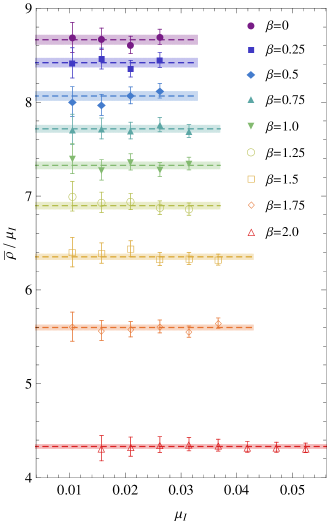
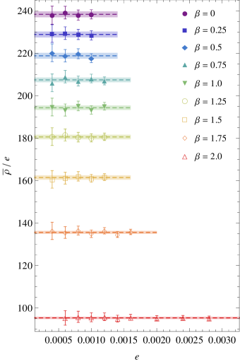
Figure 7: Ratios between the crossover parameter and the strength of perturbation: $\bar{\rho}/\mu_{\mathrm{I}}$ for the SU(2)+ICP model (left) and $\bar{\rho}/e$ for the SU(2)$\times$U(1) model (right), on $V=6^{4}$ and at various $\beta$. Colored dashed lines and strips represent the weighted averages and combined errors of the ratios.

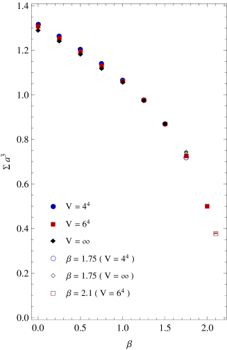
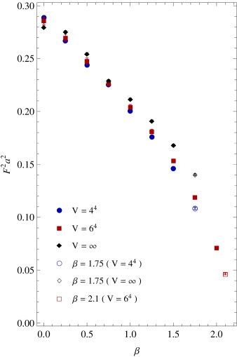
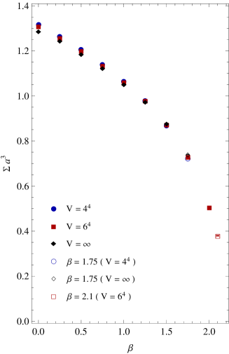
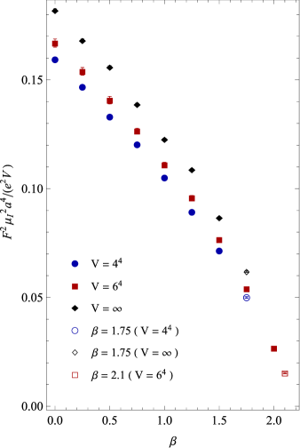
Figure 8: Coupling dependence of low-energy constants $\Sigma$ (left) and $F^{2}$ (right) derived from the SU(2)+ICP model (top) and from the SU(2)$\times$U(1) model (bottom). Blue and red filled symbols represent the values on $V=4^{4}$ and $6^{4}$, and black filled symbols their extrapolated values to $V\to\infty$. Empty symbols correspond to the cases marked $*$ in Tables 1–7 (using limited ranges for fitting $P_{k}(s)$) and extrapolations thereof.

4 Conclusions

We have analytically evaluated the $k$th smallest eigenvalue distributions $p_{k}(s)$ for a random matrix ensemble interpolating chGSE and chGUE using a Nyström-type method applied to the Fredholm Pfaffian and resolvents of the quaternion kernel. These random matrix results are applied to fit the spectra of fundamental, staggered Dirac operators of SU(2) gauge theory with imaginary chemical potential and of SU(2)$\times$U(1) gauge theory on small lattices, from the strong-coupling to the near-scaling regions. Combined use of the first four nondegenerate Dirac eigenvalue distributions in place of the spectral density or the smallest eigenvalue distribution of unperturbed SU(2) gauge theory enables us to determine the chiral condensate with $\mathcal{O}(10^{-4})$ precision. Excellent one-parameter fitting of $\chi^{2}/\text{d.o.f.}<2$ between non-cumulative individual distributions and eigenvalue histograms is achieved for almost all cases of U(1) perturbations. Combined use of the first four eigenvalue distributions also contributed to a reduction of the errors in the crossover parameter $\rho$. The acute sensitivity of $p_{k}(s)$ on $\rho$, and the observed linear dependence of $\rho$ on the perturbation strength (AB flux $\varphi$ or U(1) coupling $e$) resulted in determination of the pseudo-scalar decay constant $F$ (i.e., the coefficient of the pseudoreality-breaking term) with $\mathcal{O}(10^{-3})$ precision.

Our method of determining $F$ in QCD-like theories, which has proved to be feasible on relatively small-sized lattices, is clearly advantageous over the conventional method of using axial current correlators, which inevitably requires a large temporal dimension. A possible application of our method would be towards technicolor candidate gauge theories with fermions in (pseudo)real representations, such as SU($N$) gauge theory with two adjoint flavors Hietanen09 , which corresponds to the chGSE class if simulated with an overlap Dirac operator Ver94 . Hyper-precise determination of its “low-energy” constants (i.e., Higgs couplings) from lattice simulations using our ICP method would, upon comparison with knowledge from collider experiments, contribute to single out a credible scenario from such BSM candidates.

References

- (1) M. R. Zirnbauer, J. Math. Phys. 37, 4986 (1996).
- (2) S. Müller, S. Heusler, A. Altland, P. Braun, and F. Haake, New J. Phys. 11, 103025 (2009).
- (3) F. J. Dyson, J. Math. Phys. 3, 1191 (1962).
- (4) N. Dupuis and G. Montambaux, Phys. Rev. B 43, 14390 (1991).
- (5) K. Saito, T. Nagao, S. Müller, and P. Braun, J. Phys. A: Math. Theor. 42, 495101 (2009).
- (6) E. V. Shuryak and J. J. M. Verbaarschot, Nucl. Phys. A 560, 306 (1993).
- (7) J. J. M. Verbaarschot, Phys. Rev. Lett. 72, 2531 (1994).
- (8) P. H. Damgaard, U. M. Heller, K. Splittorff, and B. Svetitsky, Phys. Rev. D 72, 091501 (2005).
- (9) P. H. Damgaard, K. Splittorff, and J. J. M. Verbaarschot, Phys. Rev. Lett. 105, 162002 (2010).
- (10) S. M. Nishigaki, Prog. Theor. Phys. 128, 1283 (2012).
- (11) S. M. Nishigaki, Phys. Rev. D 86, 114505 (2012).
- (12) P. H. Damgaard and S. M. Nishigaki, Phys. Rev. D 63, 045012 (2001).
- (13) S. M. Nishigaki and T. Yamamoto, PoS LATTICE 2014, 067 (2014).
- (14) P. J. Forrester, T. Nagao, and G. Honner, Nucl. Phys. B 553, 601 (1999).
- (15) T. Nagao and P. J. Forrester, Nucl. Phys. B 563, 547 (1999).
- (16) T. Nagao, Random Matrices: An Introduction (University of Tokyo Press, Tokyo, 2005).
- (17) F. Bornemann, Math. Comp. 79, 871 (2010).
- (18) F. Bornemann, Markov Processes Relat. Fields 16, 803 (2010).
- (19) S. M. Nishigaki, PoS LATTICE 2015, 057 (2015).
- (20) F. A. Berezin and F. I. Karpelevich, Math. USSR-Sbornik 6, 185 (1968).
- (21) T. Guhr and T. Wettig, J. Math. Phys. 37, 6395 (1996).
- (22) A. D. Jackson, M. K. Şener, and J. J. M. Verbaarschot, Phys. Lett. B 387, 355 (1996).
- (23) M. L. Mehta, Random Matrices (Elsevier, New York, 2004), 3rd ed.
- (24) F. J. Dyson, Commun. Math. Phys. 19, 235 (1970).
- (25) T. Nagao and M. Wadati, J. Phys. Soc. Jpn. 61, 1910 (1992).
- (26) K. Frahm and J.-L. Pichard, J. Phys. 5, 847, 877 (1995).
- (27) J. B. Kogut, M. A. Stephanov, D. Toublan, J. J. M. Verbaarschot, and A. Zhitnitsky, Nucl. Phys. B 582, 477 (2000).
- (28) G. V. Dunne and S. M. Nishigaki, Nucl. Phys. B 654, 445 (2003).
- (29) K. B. Efetov, Supersymmetry in Disorder and Chaos (Cambridge University Press, Cambridge, UK, 1997).
- (30) M. A. Halasz, J. C. Osborn, and J. J. M. Verbaarschot, Phys. Rev. D 56, 7059 (1997).
- (31) T. Blum, T. Doi, M. Hayakawa, T. Izubuchi, and N. Yamada, Phys. Rev. D 76, 114508 (2007).
- (32) C. T. Sachrajda and G. Villadoro, Phys. Lett. B 609, 73 (2005).
- (33) T. Mehen and B. C. Tiburzi, Phys. Rev. D 72, 014501 (2005).
- (34) M. A. Halasz and J. J. M. Verbaarschot, Phys. Rev. Lett. 74, 3920 (1995).
- (35) A. Hietanen, J. Rantaharju, K. Rummukainen, and K. Tuominen, Nucl. Phys. B 820, 1191c (2009).