Partonic quasi-distributions of the proton and pion
from transverse-momentum distributions

Abstract

The parton quasi-distribution functions (QDFs) of Ji have been found by Radyushkin to be directly related to the transverse momentum distributions (TMDs), to the pseudo-distributions, and to the Ioffe-time distributions (ITDs). This makes the QDF results at finite longitudinal momentum of the hadron interesting in their own right. Moreover, the QDF-TMD relation provides a gateway to the pertinent QCD evolution, with respect to the resolution scale $Q$, for the QDFs. Using the Kwieciński evolution equations and well established parameterizations at a low initial scale, we analyze the QCD evolution of quark and gluon QDF components of the proton and the pion. We discuss the resulting breaking of the longitudinal-transverse factorization and show that it has little impact on QDFs at the relatively low scales presently accessible on the lattice, but the effect is visible in reduced ITDs at sufficiently large values of the Ioffe time. Sum rules involving derivatives of ITDs and moments of the parton distribution functions (PDFs) are applied to the ETMC lattice data. This allows us for a lattice determination of the transverse-momentum width of the TMDs from QDF studies.

I Introduction

Partonic structure of hadrons is vividly exemplified experimentally by the inclusive and semi-inclusive deep inelastic scattering, Drell-Yan processes, the prompt-photon emission, etc., where abundant information has been collected over the last 50 years. While parton distributions are genuinely non-perturbative objects, the scaling violations, as dictated by perturbative QCD (pQCD) radiative corrections describing the relative scale dependence of the corresponding partonic distributions, have been a major and lasting success of the theory at sufficiently high resolution Collins (2013). This verification does not account for the absolute scale dependence of parton distribution functions (PDFs), which are non-perturbative objects.

Sound but isolated attempts have been undertaken on the transverse lattice, formulated directly on the light cone Burkardt and Seal (2002); Dalley and van de Sande (2003) (for a review see, e.g., Burkardt and Dalley (2002)), which have incomprehensibly been abandoned or forgotten. On the other hand, direct ab initio calculations involving Euclidean lattices are precluded by the very Minkowski nature of PDFs (the light-cone condition in the Minkowski space $t^{2}-z^{2}=0$ shrinks to one point, $t_{E}^{2}+z^{2}=0$ in the Euclidean space where $t_{E}=it$) and the unavoidable Lorentz symmetry breaking of the finite lattice. Under those conditions, the only available method for many years has been the computation of the lowest moments of PDFs in the Bjorken $x$ variable. Along this computational strategy, transverse momentum distributions (TMDs) on the lattice were pursued by Musch et al. Musch et al. (2011) in a pioneering and comprehensive investigation.

A more recent and promising breakthrough comes from an original proposal by Ji Ji (2013), which provides an alternative route to access PDFs directly from the Euclidean lattices and relies on the so-called quasi-parton distribution functions (QDFs). These matrix elements of partonic bilinears taken between hadron states moving at a finite momentum $P_{3}$ were introduced as auxiliary objects. They involve boosting space-like correlators to a finite momentum and, eventually, may be used to extrapolate the results to the infinite-momentum frame, $P_{3}\to\infty$, yielding PDFs. Many theoretical discussions Xiong et al. (2014); Ji (2014); Ma and Qiu (2014); Ji and Zhang (2015); Ji et al. (2015); Radyushkin (2017a); Monahan and Orginos (2017); Chen et al. (2017); Ji et al. (2017); Chen et al. (2018); Carlson and Freid (2017); Briceño et al. (2017); Rossi and Testa (2017); Stewart and Zhao (2017); Radyushkin (2017b), lattice simulations Alexandrou et al. (2015, 2016, 2017a, ); Orginos et al. (2017) and quark-diquark model calculations Gamberg et al. (2015) have been undertaken along these lines.

Quite generally, the full partonic structure contains both the longitudinal and transverse information, which can equivalently be described in terms of different kinematic variables. Fourier transformations generate a proliferation of possible definitions of these objects, depending on the chosen variables, whereas relativistic covariance provides relations between them (for instance, transversity relations, connecting the Light-Cone (LC) and Equal-Time (ET) wave functions of the pion Miller and Tiburzi (2010); Broniowski et al. (2010); Ruiz Arriola and Broniowski (2010); Miller (2010)).

In a series of remarkable and insightful papers, Radyushkin Radyushkin (2017a, c, d, e) unveiled a fundamental connection between Ji’s QDFs and the well-studied TMDs Collins (2013) (see, e.g., Angeles-Martinez et al. (2015) for an overview) and the honorable Ioffe-time-distributions (ITDs) Ioffe (1969); Braun et al. (1995). The relation follows just from the Lorentz covariance (and from projecting out the subleading twist structures). This observation has triggered incipient further works on the lattice Orginos et al. (2017); Karpie et al. (2017); Monahan and Orginos providing in addition a different and upgraded perspective to former TMD lattice studies Musch et al. (2011). These crucial findings show that QDFs are in fact complementary to TMDs, thus QDFs, even at low values of $P_{3}$, should not be viewed as mere auxiliary mathematical devices, but rather as physical objects interesting in their own right. The wealth of information on TMDs from phenomenological studies in the so-called $k_{T}$-factorization scheme is therefore inherited by QDFs. Besides, this connection provides a handle on the issue of the resolution scale dependence, since much is already known on TMDs from the pQCD evolution aspect. Moreover, the results for QDFs at finite $P_{3}$ are interesting for testing non-perturbative models of the proton and pion structure.

Within the standard folklore of the TMD phenomenological studies, the independence of the longitudinal and transverse dynamics has been implemented through a Gaussian factorization ansatz, which a fortiori complies to the Drell-Yan D’Alesio and Murgia (2004) and semi-inclusive deep-inelastic scattering investigations Schweitzer et al. (2010), as well as to the recent lattice studies Musch et al. (2011). This important issue has recently been reanalyzed and confirmed for the ITDs on the quenched lattice Orginos et al. (2017); Karpie et al. (2017).

The purpose of this paper is to discuss certain aspects of the QDF-TMD connection which are potentially relevant for phenomenological and lattice studies, but have not yet been covered to sufficient detail in the literature. A careful scrutiny of the longitudinal-transverse factorization is one of the key issues we present here. Thanks to the Radyushkin QDF-TMD relation, one may investigate the QCD evolution of QDFs with a probing scale $Q$ via the known methods of the TMD evolution. Specifically, we use here a simple scheme based on the Ciafaloni, Catani, Fiorani, and Marchesini (CCFM) framework Ciafaloni (1988); Catani et al. (1990a, b), developed long ago for the then so-called $k_{T}$-unintegrated gluon distributions to evolve TMDs. The CCFM equations in the single loop approximation were later adapted to include quarks by Kwieciński Kwiecinski (2002) (see also Gawron and Kwiecinski (2003); Gawron et al. (2003); Ruiz Arriola and Broniowski (2004)). We use the solutions of the Kwieciński evolution equations for both the proton and the pion, where the initial condition for the evolution imposed at the scale $Q_{0}$ is obtained by assuming a factorized ansatz involving a known parametrization of the PDFs and a choice of the transverse-coordinate profile function. We bring up the fact that the QCD evolution of TMDs precludes factorization at all scales. However, the induced breaking does not generate a large effect on the QDFs at the relatively low values of $Q\sim 2$ GeV, which are presently available on the lattice.

The factorization breaking from the QCD evolution is visible in ITDs at magnitudes of the Ioffe time above several units, thus in the tail, which via Fourier transform corresponds to low values of $x$. Therefore, the factorization breaking becomes relevant at low values of $x$ and is enhanced at higher values of $Q$. Note, however, that the low-$x$ domain is not accessible to the methodology of the present Euclidean lattice investigations. We also explore the reduced ITDs proposed in Orginos et al. (2017), which are specifically designed to probe the longitudinal-transverse factorization. With the factorization breaking induced by the Kwieciński evolution, we find effects in the tails of the reduced ITDs, which become increasingly relevant as the value of the longitudinal momentum of the hadron is reduced.

In our study, we provide QDFs for both quarks and gluons in the proton and the pion, as well as the corresponding ITDs. One should keep in mind, however, that an evaluation of the gluon distributions on the lattice is more demanding than for the quark case.

On the general ground, we spell out simple sum rules linking the derivatives of ITDs at the origin to the $x$-moments of the PDFs and the moments of the $k_{T}$ distribution. These sum rules may be useful for consistency checks of the lattice results. For the reduced ITDs, they set the slope of the imaginary part and the curvature of the real part at the origin, which are universal, and determined by the first and second $x$-moment of the corresponding PDF. They also link in a simple way the $x$ moments of the QDFs and PDFs, and the $k_{T}$ moments of TMDs. We have applied the sum rules to the lattice data of Alexandrou et al. (2016), confirming proper scaling with $P_{3}$ and extracting the with of the $k_{T}$ distribution.

II Definitions and relations

We begin by presenting a glossary of relevant definitions and formulas. The results referring to the Ioffe distributions and the link between QDFs and TMDs were obtained in previous works Braun et al. (1995); Radyushkin (2017a, d); Orginos et al. (2017). We review them here for completeness and to establish our notation.

II.1 Quark distributions

The Lorentz covariance allows one to parametrize the matrix elements of the spin-averaged quark bilinears as

$$\langle P|\bar{\psi}(0)\gamma^{\mu}U[0,z]\psi(z)|P\rangle$$

$$=P^{\mu}h(P\cdot z,z^{2})+z^{\mu}h_{z}(P\cdot z,z^{2}),$$ (1)

where $|P\rangle$ is a hadron state of four-momentum $P$, the link operator, providing the gauge invariance, is denoted as $U[0,z]$, and $h(P\cdot z,z^{2})$ and $h_{z}(P\cdot z,z^{2})$ are scalar functions. The term proportional to $z^{\mu}$ in the decomposition of Eq. (1) contains subleading twist pieces only, so it is favorable to project it out from the following definitions Radyushkin (2017a, d). The issue is discussed in some greater detail in Appendix A.

Following Radyushkin (2017a, d); Orginos et al. (2017), we define the parton quasi-distributions (QDFs) analogously to the original proposal by Ji Ji (2013), but retaining the $P^{\mu}$ term only, i.e.,

$$\tilde{q}(y,P_{3})=P_{3}\int\frac{dz_{3}}{2\pi}e^{-iyP_{3}z_{3}}h(-P_{3}z_{3},-z_{3}^{2}).$$ (2)

Here $y$ acquires the interpretation of the fraction of the hadron’s longitudinal momentum $P_{3}$ carried by the parton, with the support $y\in(-\infty,\infty)$. As shown by Ji Ji (2013), in the limit of $P_{3}\to\infty$ one recovers the usual PDFs,

$$\lim_{P_{3}\to\infty}\tilde{q}(y,P_{3})=q(x=y),$$ (3)

where

$$q(x)=P_{+}\int\frac{dz_{-}}{2\pi}e^{ixP_{+}z_{-}}h(P_{+}z_{-},0),$$ (4)

with $y=x$ denoting the fraction of the light-front momentum of the hadron carried by the parton.

More precisely, in the adopted convention the distribution for $x\in[0,1]$ corresponds to the quarks, and for $x\in[-1,0]$ to the anti-quarks, i.e., $\bar{q}(x)=-q(-x)$ Jaffe (1983) (see Ref. Jaffe (1985) for a pedagogical introduction). Then, for the valence and sea quarks one has

$$q_{\rm val}(x)=q(x)-\bar{q}(x)=q(x)+q(-x),\;\;\;\ x\in[0,1],$$

$$q_{\rm sea}(x)=\left\{\begin{array}[]{cl}\bar{q}(x)=-q(-x)&\;\;\;\ {\rm for~{}~{}}x\in[0,1],\\ -\bar{q}(-x)=q(x)&\;\;\;\ {\rm for~{}~{}}x\in[-1,0].\end{array}\right.$$ (7)

The transverse-momentum unintegrated parton distribution, or TMD, is defined as

$$q(x,k_{1},k_{2}) \equiv P^{+}\!\!\!\int\frac{dz^{-}}{2\pi}e^{ixP_{+}z_{-}}\!\!\!\int\frac{dz_{1}}{2\pi}e^{ik_{1}z_{1}}\!\!\!\int\frac{dz_{2}}{2\pi}e^{ik_{2}z_{2}}$$ (8)

$$\times h(P_{+}z_{-},-z_{1}^{2}-z_{2}^{2}).$$

From the axial symmetry $q(x,k_{1},k_{2})=q(x,k_{T}^{2})$, with $\vec{k}_{T}=(k_{1},k_{2})$.

II.2 Gluon distributions

For the gluons, the corresponding matrix element can be defined analogously as

$$\langle P|F^{\mu\alpha}(0)U[0,z]{F_{\alpha}}^{\nu}(z)|P\rangle z_{\mu}z_{\nu}$$

$$=P^{\mu}P^{\nu}h_{g}(P\cdot z,z^{2})+\dots,$$ (9)

with the dots denoting terms containing higher twists only, and the QDF and PDF, multiplied by the corresponding momentum fractions, are defined as

$$y\tilde{g}(y,P_{3})=P_{3}\int\frac{dz_{3}}{2\pi}e^{-iyP_{3}z_{3}}h_{g}(-P_{3}z_{3},-z_{3}^{2}),$$

$$xg(x)=P_{+}\int\frac{dz_{-}}{4\pi}e^{ixP_{+}z_{-}}h_{g}(P_{+}z_{-},0).$$ (10)

The quasi-distribution $y\tilde{g}(y,P_{3})$ is distributed symmetrically in $y\in(-\infty,\infty)$, whereas $xg(x)$ is distributed symmetrically in the domain $x\in[-1,1]$ (see, e.g., Refs. Ji (1998) for discussion). Then, together with the quark and antiquark distributions they form the singlet component of the partonic distributions in context of their QCD evolution.

II.3 Transversity relations

Lorentz invariance of the matrix elements allows one to obtain relations, which otherwise are a priori not obvious. To our knowledge, the first investigations along these lines were done in Miller and Tiburzi (2010); Broniowski et al. (2010); Ruiz Arriola and Broniowski (2010); Miller (2010) for the case of the pion wave function (see Appendix B for a brief review). The functions $\Phi_{a}(\alpha,z^{2})$ of Eq. (57) are analogs of the pseudo-distributions introduced by Radyushkin Radyushkin (2017c) and advocated as a basic entity of the formalism.

Note that the functional dependence in both integrands appearing in the QDF in Eq. (2) and the TMD in Eq. (8) suggests a direct link. Radyushkin Radyushkin (2017a) showed that QDFs are simply but non-trivially related to TMDs,

$$\tilde{q}(y,P_{3})=P_{3}\int dk_{1}\!\!\int dx\,q(x,k_{1}^{2}+(x-y)^{2}P_{3}^{2}).$$ (11)

For completeness, in Appendix C we review the derivation of the Radyushkin relation from the Lorentz invariance Radyushkin (2017c) in an explicit manner.

We may use the transverse coordinate representation (Fourier-conjugate to definition (8) and denoted with a hat) of the TMD,

$$\hat{q}(x,z_{T}^{2})=\!\!\!\int\frac{d\nu}{2\pi}e^{-i\nu x}h(-\nu,-z_{T}^{2}),$$ (12)

where the transverse coordinate is $z_{T}=(0,z_{2})$, whereas the integration variable $\nu=-P\cdot z$ is the Ioffe time Ioffe (1969); Braun et al. (1995). In the Lorentz-invariant notation one recovers Radyushkin’s pseudo-distribution ${\cal P}$ Radyushkin (2017c)

$$\hat{q}(x,-z^{2})\equiv{\cal P}(x,-z^{2})=\!\!\!\int\frac{d\nu}{2\pi}e^{-i\nu x}h(-\nu,z^{2}),$$ (13)

which in the frame $z=(0,0,0,z_{3}$) applied below becomes

$$\hat{q}(x,z_{3}^{2})={\cal P}(x,z_{3}^{2})=\!\!\!\int\frac{d\nu}{2\pi}e^{-i\nu x}h(-\nu,-z_{3}^{2}).$$ (14)

We can now write down an equivalent form of Eq. (11), which links QDF to TMD or to the pseudo-distribution, namely

$$\tilde{q}(y,P_{3}) = P_{3}\int dx\int\frac{dz_{2}}{2\pi}e^{-i(y-x)z_{2}P_{3}}\hat{q}(x,z_{T}^{2})$$ (15)

$$= P_{3}\int dx\int\frac{dz_{3}}{2\pi}e^{-i(y-x)z_{2}P_{3}}\hat{q}(x,z_{3}^{2}).$$

These relations can be inverted if we invoke the integration over $P_{3}$:

$$\hat{q}(x,z_{T}^{2})=z_{2}\int dy\,\int dP_{3}e^{i(y-x)z_{2}P_{3}}\tilde{q}(y,P_{3}),$$

$$\hat{q}(x,z_{3}^{2})=z_{3}\int dy\,\int dP_{3}e^{i(y-x)z_{3}P_{3}}\tilde{q}(y,P_{3}).$$ (16)

Therefore the knowledge of quasi-distributions at all values of the hadron momentum $P_{3}$ allows one for obtaining the corresponding TMD and the pseudo-distribution in $z_{3}$.

The matrix element $h(-\nu,z^{2})$ appearing in Eq. (14) is referred to as the Ioffe-time distribution (ITD) Braun et al. (1995); Orginos et al. (2017), and is equal to $2{\cal M}_{p}(\nu,-z^{2})$ in the notation of Radyushkin (2017a, d). The normalized amplitude Musch et al. (2011), or the reduced  ITD Orginos et al. (2017), used to probe the transverse-longitudinal factorization, is defined as

$$\mathfrak{M}(\nu,-z^{2})=\frac{{\cal M}_{p}(\nu,-z^{2})}{{\cal M}_{p}(0,-z^{2})}=\frac{h(-\nu,z^{2})}{h(0,z^{2})}.$$ (17)

The denominator has an interpretation of the rest-frame distribution.

This definition has the advantage that the self-energy of the Wilson loop characterized by a multiplicative renormalization factor $\sim e^{-z_{3}m}$ cancels in the ratio. This finding on the lattice Orginos et al. (2017) is in harmony with the improved parton quasi-distribution through the Wilson line renormalization Chen et al. (2017), which safely removes power divergences ubiquitous in lattice QCD.

III Sum rules for the matrix elements of bilocal fields

Fourier inversion with $\nu=-P_{3}z_{3}$ of Eq. (14) yields the relation of the ITD with the pseudo-distribution,

$$h(-P_{3}z_{3},-z_{3}^{2})=\int_{-1}^{1}{dx}\,e^{iP_{3}z_{3}x}\hat{q}(x,z_{3}^{2}),$$ (18)

whereas the corresponding inversion of Eq. (2) links ITD to QDF,

$$h(-P_{3}z_{3},-z_{3}^{2})=\int_{-\infty}^{\infty}{dy}\,e^{iP_{3}z_{3}y}\tilde{q}(y,P_{3}).$$ (19)

We immediately see that the real part of $h$ is an even function of $z_{3}$, whereas the imaginary part is odd. Note that according to Eq. (7), the valence quarks contribute both to the real and imaginary parts of $h$, the sea quarks contribute to the imaginary part of $h$ only, and the gluons yield $h_{g}$ which is real. Also, Eqs. (18) and (19) immediately yield the equality

$$\int_{-1}^{1}{dx}\,e^{iP_{3}z_{3}x}\hat{q}(x,z_{3}^{2})=\int_{-\infty}^{\infty}{dy}\,e^{iP_{3}z_{3}y}\tilde{q}(y,P_{3}),$$ (20)

which leads to the new sum rules presented shortly.

The normalization condition for the quark PDF yields, from Eqs. (18,19),

$$h(0,0)=\int_{-1}^{1}\!\!{dx}\,\hat{q}(x,0)=\int_{-1}^{1}\!\!{dx}\,q(x)$$

$$=\int_{-\infty}^{\infty}\!\!{dy}\,\tilde{q}(y,P_{3})=N_{q},$$ (21)

where $N_{q}$ is the number of valence quarks of a given flavor.

Taking subsequent derivatives of the left- and right-hand sides of Eq. (20) with respect to $z_{3}$ at the origin, under the assumption of regularity of $\hat{q}(x,z_{3}^{2})$ in $z_{3}^{2}$, yields simple sum rules which depend parametrically on $P_{3}$.

The first derivative of Eq. (20) is related to fractions of momenta carried by the quarks,

$$\left.\frac{d}{dz_{3}}h(-P_{3}z_{3},-z_{3}^{2})\right|_{z_{3}=0}$$

$$=iP_{3}\int_{-1}^{1}\!\!{dx}\,x\,q(x)=iP_{3}\int_{-\infty}^{\infty}\!\!{dy}\,y\,\tilde{q}(y,P_{3})$$ (22)

(we have used the fact that $\left.{d}\hat{q}(x,z_{3}^{2})/{dz_{3}}\right|_{z_{3}=0}=0$, which follows from regularity), or

$$\langle x\rangle_{q}=\langle y\rangle_{q}(P_{3})=\langle y\rangle_{q}$$ (23)

(the brackets denote the moments appearing in Eq. (22)).

We notice from Eq. (22) that the derivative of the imaginary part of $h$ with respect to $z_{3}$ at the origin is proportional to $P_{3}$ and contains a known coefficient, $\langle x\rangle_{q}$. We also note that the first $y$-moment of $\tilde{q}(y,P_{3})$, which in principle might depend on $P_{3}$, in fact does not, as indicated in Eq. (23).

Similarly, the second derivative of Eq. (20) with respect to $z_{3}$ at the origin yields

$$\left.\frac{d^{2}}{dz_{3}^{2}}h(-P_{3}z_{3},-z_{3}^{2})\right|_{z_{3}=0}$$ (24)

$$=-P_{3}^{2}\int_{-1}^{1}\!\!{dx}\,x^{2}q(x)+\int_{-1}^{1}\!\!{dx}\,\left.\frac{d^{2}}{dz_{3}^{2}}\hat{q}(x,z_{3}^{2})\right|_{z_{3}=0}$$

$$=-P_{3}^{2}\int_{-\infty}^{\infty}\!\!{dy}\,y^{2}\tilde{q}(y,P_{3}).$$

Since the quasi-distributions and the TMDs have the same functional form, their Maclaurin expansions, correspondingly, in $z_{3}$ or $z_{2}$ are the same. The interpretation of the coefficients can thus be given via the ($x$-dependent) $k_{T}$-moments of the TMDs. In particular, for the quadratic term we have

$$\left.\frac{d^{2}}{dz_{3}^{2}}\hat{q}(x,z_{3}^{2})\right|_{z_{3}=0}=\left.\frac{d^{2}}{dz_{2}^{2}}\hat{q}(x,z_{2}^{2})\right|_{z_{2}=0}$$

$$=-\frac{1}{2}P_{3}^{2}\langle k_{T}^{2}\rangle(x)\,q(x).$$ (25)

We introduce the short-hand notation for the $x$-averaged $k_{T}$ width per valence quark,

$$\overline{\langle k_{T}^{2}\rangle}=\int_{-1}^{1}\!{dx}\langle k_{T}^{2}\rangle(x)q(x)/N_{q}.$$ (26)

We may now rewrite Eq. (24) in a compact form

$$\langle x^{2}\rangle_{q}+\frac{N_{q}\overline{\langle k_{T}^{2}\rangle}}{2P_{3}^{2}}=\langle y^{2}\rangle_{q}(P_{3}).$$ (27)

We note from Eq. (24) that increasing $P_{3}$ makes the function $h$ more and more sharply peaked at the origin. Also, the width of QDF is larger than the width of the corresponding PDF, as follows from the relation of the second moments (27), with the first moments being equal, cf. Eq. (23). The effect is of the order $\overline{\langle k_{T}^{2}\rangle}/P_{3}^{2}$,

Higher-order relations may be readily obtained taking more differentiations with respect to $z_{3}$, and hold as long as the obtained moments exist.

For the gluon distributions, analogously,

$$h_{g}(0,0)=\langle x\rangle_{g}=\langle y\rangle_{g},$$

$$\left.\frac{d}{dz_{3}}h_{g}(-P_{3}z_{3},-z_{3}^{2})\right|_{z_{3}=0}=0,$$ (28)

and

$$\left.\frac{d^{2}}{dz_{3}^{2}}h_{g}(-P_{3}z_{3},-z_{3}^{2})\right|_{z_{3}=0}$$ (29)

$$=-P_{3}^{2}\langle x^{3}\rangle_{g}-\frac{1}{2}\int_{-1}^{1}\!\!{dx}\langle k_{T}^{2}(x)\rangle_{g}xg(x)=-P_{3}^{2}\langle y^{3}\rangle_{g}(P_{3}).$$

Equations (22-29) may have a practical significance in the interpretation and consistency checks of the lattice data. The consistency can be verified by checking the $P_{3}$ dependence in Eq. (23) with the known $x$-moment. Equations (27,29) provide a way to effectively measure the average spreading of the transverse momentum in the TMDs. One would need to obtain the matrix elements $h$ or $h_{g}$ at various values of $P_{3}$ with a sufficient accuracy, such that interpolation fits can be made and then derivatives at the origin taken. In Sec. VI we successfully apply the sum rules to the lattice data from Alexandrou et al. (2016).

The distributions in the Ioffe time $\nu=-P_{3}z_{3}$ display more universality, as then the slope of the imaginary part of $h$ at the origin is common to all values of $P_{3}$,

$$\left.\frac{d}{d\nu}h\left(-\nu,-\frac{\nu^{2}}{P_{3}^{2}}\right)\right|_{\nu=0}=i\langle x\rangle_{q}=i\langle y\rangle_{q},$$ (30)

whereas the curvature at the origin of the real part of $h$ is

$$\left.\frac{d^{2}}{d\nu^{2}}h\left(-\nu,-\frac{\nu^{2}}{P_{3}^{2}}\right)\right|_{\nu=0}\!\!\!\!\!\!=-\langle x^{2}\rangle_{q}-\frac{N_{q}\overline{\langle k_{T}^{2}\rangle}}{2P_{3}^{2}}=-\langle y^{2}\rangle_{q}(P_{3}).$$

(31)

Above, we have used the same method as in the derivation of Eq. (23,27).

There is even more vivid universality for the reduced ITDs, where both first and second derivatives at the origin are independent of $P_{3}$:

$$\left.\frac{d}{d\nu}\mathfrak{M}(\nu,\nu^{2}/P_{3}^{2})\right|_{\nu=0}=i\langle x\rangle_{q}=i\langle y\rangle_{q},$$ (32)

$$\left.\frac{d^{2}}{d\nu^{2}}\mathfrak{M}(\nu,\nu^{2}/P_{3}^{2})\right|_{\nu=0}\!\!\!\!\!\!=-\langle x^{2}\rangle_{q}=-\langle y^{2}\rangle_{q}(P_{3})+\frac{N_{q}\overline{\langle k_{T}^{2}\rangle}}{2P_{3}^{2}}.$$

The discussed universality behavior was observed in actual (quenched) lattice simulations reported in Orginos et al. (2017).

IV Factorization ansatz

In modeling of TMDs, a popular assumption is the factorization ansatz

$$q(x,k_{T})=q(x)F(k_{T}),$$ (33)

or, equivalently,

$$\hat{q}(x,z_{T})=q(x)\hat{F}(z_{T}),$$ (34)

which separates the transverse and longitudinal dynamics (we will discuss later on the departures from this assumption). Whereas this has traditionally been an out-of-ignorance guess, lattice calculations of TMDs speak in favor of this factorization, at least as long as $m_{\pi}\simeq 600~{}{\rm MeV}$ Musch et al. (2011). Moreover, one typically uses a Gaussian shape

$$F(k_{T})=\frac{e^{-\frac{k_{T}^{2}}{\langle k_{T}^{2}\rangle}}}{\pi\langle k_{T}^{2}\rangle},\;\;\hat{F}(z_{T})=e^{-\frac{z_{T}^{2}}{2\sigma_{0}^{2}}},\;\;\sigma_{0}^{2}=\frac{2}{\langle k_{T}^{2}\rangle}.$$ (35)

The Gaussian factorization ansatz has been favorably checked against the data in the Drell-Yan D’Alesio and Murgia (2004) and semi-inclusive deep-inelastic scattering Schweitzer et al. (2010). In the context of quasi-distributions, this form was explored in Radyushkin (2017a, d); Orginos et al. (2017). A typical value of $\langle k_{T}^{2}\rangle$ extracted from phenomenological studies (at energy scales of a few GeV) is $\langle k_{T}^{2}\rangle\sim 0.3-0.6~{}{\rm GeV}^{2}$ Melis (2015); Bacchetta et al. (2017).

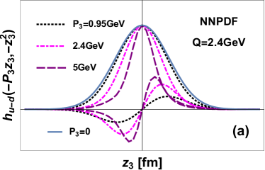
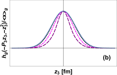
Figure 1: Matrix element corresponding to the (a) quark (b) gluon QDF of the proton for several values of $P_{3}$, evaluated in the factorization model, where the PDFs at the scale $Q=2.4$ GeV, taken from the NNPDF parametrization, are supplied with a Gaussian form factor with the width parameter $\langle k_{T}^{2}\rangle=0.6$ GeV. The real parts are symmetric in $z_{3}$, whereas the imaginary parts are antisymmetric. The solid line ($P_{3}=0$) indicates the form factor $\hat{F}(z_{3}^{2})$.

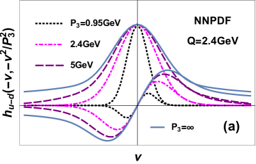
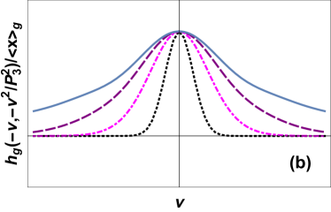
Figure 2: Same as in Fig. 1 but for the the distributions in the Ioffe time $\nu=P_{3}z_{3}$. In this case the solid lines labeled $P_{3}=\infty$ represent the limits of Eq. (42).

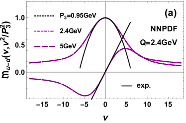
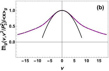
Figure 3: Same as in Fig. 1 but for the reduced ITDs of the proton, $\mathfrak{M}$, of Eq. (17). The straight or parabolic solid lines indicate the leading expansion at $\nu=0$, as explained in the text. The model curves at various values of $P_{3}$ overlap, displaying universality.

With the factorization (34), Eq. (15) becomes the folding formula

$$\tilde{q}(y,P_{3})=P_{3}\int dxF[(x-y)P_{3}]\,q(x)$$ (36)

of the form factor $F[(x-y)P_{3}]$ and the PDF. Equation (36) carries a particular “operational” simplicity: in the factorized case, QDF is obtained from PDF in terms of a simple folding, which washes out the PDF, more and more as $P_{3}$ is decreased. On the other hand, when $P_{3}\to\infty$, the form factor tends to the delta function and QDF approaches PDF, in agreement with Eq. (3).

With the Gaussian form (35) one has

$$\tilde{q}(y,P_{3})=\frac{1}{\sqrt{2\pi}\Sigma}\int dx\,e^{-\frac{(x-y)^{2}}{2\Sigma^{2}}}q(x),$$ (37)

where

$$\Sigma^{2}=\frac{1}{\sigma_{0}^{2}P_{3}^{2}}=\frac{\langle k_{T}^{2}\rangle}{2P_{3}^{2}}.$$ (38)

The effective parameter of the mentioned washing-out is thus the ratio $\Sigma^{2}$ from Eq. (38).

In the factorization approximation Eq. (19) becomes

$$h(-P_{3}z_{3},-z_{3}^{2})=\hat{F}(z_{3}^{2})\int{dx}\,e^{iP_{3}z_{3}x}q(x),$$ (39)

hence

$$h(0,-z_{3}^{2})=\hat{F}(z_{3}^{2})$$ (40)

and

$$\mathfrak{M}(\nu,\nu^{2}/P_{3}^{2})=\int{dx}\,e^{i\nu x}q(x)$$ (41)

becomes a universal ($P_{3}$-independent) function.

In the limit of $P_{3}\to\infty$, the ITDs also loose the information on the form factor, as then

$$h(-\nu,-\nu^{2}/P_{3}^{2})\to h(-\nu,0)=\int{dx}\,e^{i\nu x}q(x),$$ (42)

which gives exactly the same form as Eq. (41). Note that the form factor $\hat{F}(z_{3}^{2})$ cancels also from the ratio of the imaginary and real parts,

$$\frac{{\rm Im}\,h(-P_{3}z_{3},-z_{3}^{2})}{{\rm Re}\,h(-P_{3}z_{3},-z_{3}^{2})}=\frac{\int{dx}\,\sin(P_{3}z_{3}x)q(x)}{\int{dx}\,\cos(P_{3}z_{3}x)q(x)},$$ (43)

which also provides a measure of goodness of the factorization ansatz.

In the factorization ansatz, Eq. (27) takes a simple form, where the width of the transverse-momentum distribution of partons is independent of $x$:

$$\left.\frac{d^{2}}{dz_{3}^{2}}h(-P_{3}z_{3},-z_{3}^{2})\right|_{z_{3}=0}=-P_{3}^{2}\langle x^{2}\rangle_{q}-\frac{1}{2}{N_{q}}\langle k_{T}^{2}\rangle,$$ (44)

For the gluon distribution analogous results to those listed above are immediately obtained.

The remainder of this Section is devoted to an illustration of the derived results in a sample calculation. We evaluate the matrix elements $h$ and $h_{g}$ using the NNPDF parametrization of the PDFs of the proton in the factorization model. As the scale, we take $Q=2.4$ GeV, which corresponds to the lattice spacing of 0.08 fm used in Alexandrou et al. (2015, 2017a, ). The factorization ansatz (34) with a Gaussian form factor (35) is assumed to hold at this scale. We take $\langle k_{T}^{2}\rangle=0.6~{}{\rm GeV}^{2}$ for both the quarks and gluons.

In Fig. 1 we plot the matrix element for the difference of $u$ and $d$ quarks, $h_{u-d}(-P_{3}z_{3},-z_{3}^{2})$, and $h_{g}(-P_{3}z_{3},-z_{3}^{2})$, evaluated at several values of $P_{3}$ (the values $P_{3}=0.95$ GeV and 2.4 GeV were used in Alexandrou et al. (2015, 2017a, )). The solid line represents the limit of $P_{3}=0$, where $h(0,-z_{3}^{2})=h_{g}(0,-z_{3}^{2})/\langle x\rangle_{g}=\hat{F}(z_{3}^{2})$. We notice clearly the features of Eqs. (23,44), with the slope of the imaginary parts increasing with $P_{3}$, and the real parts becoming more and more sharply peaked at the origin.

Figure 2 presents the analogous results for ITDs. Here the solid lines correspond to the $P_{3}\to\infty$ limit, i.e., the distributions $h(-\nu,0)$ or $h_{g}(-\nu,0)$ of Eq. (42). We note indeed that as $P_{3}$ increases, the curves tend to $h(-\nu,0)$ or $h_{g}(-\nu,0)$, but at large values of $\nu$ the convergence is slow.

Finally, in Fig. 3 we show the reduced ITDs, which in the factorization ansatz are universal (independent of $P_{3}$) functions. Note that according to Eqs. (41) and (42), these are the same curves as the $P_{3}\to\infty$ lines from Fig. 2. The straight or parabolic solid lines in Fig. 3 represent the expansion in $\nu$ up to second order, i.e., the functions $\nu\langle x\rangle_{u-d}$ and $1+\frac{1}{2}\nu^{2}\langle x\rangle_{u-d}$ for the imaginary and real parts of $h_{u-d}$, respectively, and the function $1+\frac{1}{2}\nu^{2}\langle x^{3}\rangle_{g}/\langle x\rangle_{g}$ for the case of the gluon distribution. For the presented NNPDF case, numerically, $\langle x\rangle_{u-d}=0.16$, $\langle x^{2}\rangle_{u-d}=0.05$, $\langle x\rangle_{g}=0.44$, and $\langle x^{3}\rangle_{g}=0.01$. Of course, the results conform to the sum rules of Sect. III.

The long tail in the reduced ITDs, prominently seen in Figs. 1 or 3, is immanently related to the low-$x$ behavior of the associated PDFs, which typically involve an integrable singularity as $x\to 0$. For instance, if the distribution behaves low $x$ as $x^{-\alpha}$, with $\alpha<1$, (for the moment we use distributions defined in the domain $x\in[0,1]$, which can be converted according to Eq. (7), then the asymptotic behavior of the corresponding ITDs goes as $\nu^{-1+\alpha}$. Note that this long-tail behavior in $\nu$, following from the low-$x$ behavior of the PDFs, is inaccessible on the lattice. In contrast, the simulations of Orginos et al. (2017) or Alexandrou et al. (2015, 2017a, ) display a rapid fall-off of the matrix elements to zero around $|\nu|\sim 5$–10. We believe this is associated to the lattice discretization. When $P_{3}=2\pi n/L$, with $L$ denoting the longitudinal size and $n$ being a small natural number, (typically 1–5), then $|\nu|=|P_{3}z_{3}|\leq 2\pi n$. This, in turn, via the Fourier transform, sets a lower limit for the accessible values of $x$, namely $x>\frac{1}{n}$.

Having seen that the lattice simulations cannot go to large values of $|\nu|$, a doubt arises concerning the practicality of the method. We have demonstrated that the expansion in $\nu$ near the origin, with the coefficients given by the $x$-moments of the PDFs, works. Adding some next terms with higher moments would lead to further improvement, such that the expansion would be fairly accurate up to, say, $|\nu|\sim 5$. However, since the ambition of the lattice method based on QDFs is to surpass the moment evaluations and provide the PDFs themselves as functions of $x$ (be it for sufficiently large arguments), one has to verify if the“principle of conservation of difficulty” is possible to circumvent.

V QCD evolution and the breaking of factorization

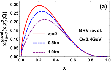
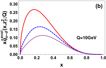
Figure 4: The $u-d$ TMDs (multiplied with $x$) in the proton, plotted as functions of the momentum fraction $x$ at various values of the transverse coordinate $z_{T}$. The model takes a factorized ansatz at the scale $Q_{0}=510$ MeV with the GRV parametrization and caries out the Kwieciński evolution with Eq. (46) to the lattice scale (a) $Q=2.4$ GeV or (b) $Q=10$ GeV.

A proper definition of PDFs, QDFs, ITDs, TMDs, etc., requires specification of the resolution scale, which we generically denote by $Q$, as it is expected to be the natural choice where the hard scale is identified with the probing momentum $Q$. Here we treat the resolution scale as an independent parameter in the problem within the $\overline{\rm MS}$-renormalization scheme in the continuum, as opposed to the discrete lattice approach to renormalization. For sufficiently fine lattices, the value of the scale can be, roughly speaking, identified with the lattice spacing expressed in physical units, $a\sim 1/Q$. When $Q$ is large enough, the pQCD approach can be invoked.

A trivial but practically relevant observation is that once we are able to carry out the QCD evolution for some representation of the partonic distribution, for instance the TMD, we can then use the integral transformations unveiled by Radyushkin and spelled out in Sect. II to effectively carry out the evolution for another representation, such as QDF. We can thus rewrite Eq. (15)

$$\tilde{q}(y,P_{3};Q)=P_{3}\!\!\int\!dx\!\int\!\frac{dz_{2}}{2\pi}e^{-i(y-x)z_{2}P_{3}}\hat{q}(x,z_{2}^{2};Q),$$ (45)

where now the dependence on the scale is explicitly indicated. Our scheme is to evolve the TMD, $\hat{q}$, and that way produce an evolved QDF or ITD. Note that in this treatment $P_{3}$ is an external (kinematic) variable.

For the standard unintegrated gluon distribution (or TMD) one has at hand the Ciafaloni, Catani, Fiorani, and Marchesini (CCFM) evolution equations Ciafaloni (1988); Catani et al. (1990a, b), which in a sense interpolate between the DGLAP Gribov and Lipatov (1972); Dokshitzer (1977); Altarelli and Parisi (1977) and BFKL Lipatov (1976); Kuraev et al. (1977); Balitsky and Lipatov (1978) methods. The CCFM scheme was extended to incorporate quarks by Kwieciński Kwiecinski (2002) in the so-called one-loop approximation. The technicalities standing behind this derivation were very precisely explained in Golec-Biernat et al. (2007), see also the review Gustafson et al. (2002), hence we do not give more details here.

For our practical purpose it is important we have a ready-to-apply method with is simple but non-trivial in the present context. Moreover, Kwieciński Kwiecinski (2002) showed that in the transverse-coordinate ($z_{T}$) representation, the one-loop CCFM equations become diagonal in $z_{T}$, possessing the structure very much like the DGLAP equations for the corresponding integrated parton distributions (PDFs), but with a modified kernel. For the non-singlet case they read

$$Q^{2}{\partial\hat{q}(x,z_{T}^{2};Q)\over\partial Q^{2}}={\alpha_{s}(Q^{2})\over 2\pi}\int_{0}^{1}d\xi\,P_{qq}(\xi)\bigg{[}\Theta(\xi-x)$$

$$\times J_{0}[(1-\xi)Qz_{T}]\,\hat{q}\left({x\over\xi},z_{T}^{2};Q\right)-\hat{q}(x,z_{T}^{2};Q)\bigg{]},$$ (46)

where $P_{qq}(\xi)$ is the usual splitting function and $J_{0}$ stands for the Bessel function. The singlet case, embodying the gluon and sea mixing as well as details and methods of solutions, can be found in Kwiecinski (2002); Gawron and Kwiecinski (2003); Gawron et al. (2003); Ruiz Arriola and Broniowski (2004).

The initial condition at the scale $Q_{0}$ is provided with a factorized form

$$\hat{q}(x,z_{T}^{2};Q_{0})=\hat{F}(z_{T}^{2})q(x;Q_{0}),$$ (47)

and evolved with Eq. (46) to the scale $Q$. Since the evolution is diagonal in $z_{T}$, the presence of $\hat{F}(z_{T}^{2})$ has only a multiplicative effect, and the evolved solution has the form

$$\hat{q}(x,z_{T}^{2};Q)=\hat{F}(z_{T}^{2})\hat{q}^{\rm evol}(x,z_{T}^{2};Q).$$ (48)

In other words, the dependence of the TMD on $z_{T}$ sits in a factorized trivial component put in by hand, $\hat{F}(z_{T}^{2})$, and a dynamically generated non-trivial component, which mixes $z_{T}$ and $x$, i.e., yields the longitudinal-transverse factorization breaking. The factorization ansatz (34), which is assumed to hold at a scale $Q_{0}$ in Eq. (47), is broken at higher scales $Q$. The breaking increases with the evolution range and, as we shall see, with decreasing $x$.

In Fig. 4 we present the solutions of Eq. (46) (we plot $\hat{q}^{\rm evol}$ parts of Eq. (48), as it shows the dynamical effect of the evolution). For this part of our analysis we take for the PDF the GRV Glück et al. (1998) initial conditions at the scale $Q_{0}=510$ MeV. For simplicity, we neglect the small effect of the isospin asymmetry of the sea quarks. At this scale we use the factorization formula (47) with a Gaussian form factor and $\langle k_{T}^{2}\rangle_{0}=0.38~{}{\rm GeV}^{2}$. This value is fixed in such a way that after the evolution to $Q=2.4$ GeV the average width is equal to the phenomenological number $\overline{\langle k_{T}^{2}\rangle}=0.57~{}{\rm GeV}^{2}$ Melis (2015). We note from Fig. 4 that an increase of $z_{T}$ leads to a decrease of the distribution, which is accelerated as $Q$ grows. Also, the shape in $x$ is not maintained when $z_{T}$ is changed. This displays the factorization breaking in an explicit manner.

The evolution of Eq. (46) leads to a substantial narrowing of the TMDs in $z_{T}$ or, equivalently, broadening in $k_{T}$, as $x$ is being decreased. The results for

$$\langle k_{T}^{2}\rangle_{u-d}(x)=\langle k_{T}^{2}\rangle_{0}+\int d^{2}k_{T}\,k_{T}^{2}q^{\rm evol}_{u-d}(x,k_{T}^{2};Q),$$ (49)

after evolution up to $Q=2.4$ GeV, are shown in Fig. 5. We note a strong dependence on $x$, with $\langle k_{T}^{2}\rangle_{u-d}(x)$ growing as $x$ decreases. At $x=1$ there is no effect, which reflects the form of the evolution kernel in Eq. (46). The average width $\overline{\langle k_{T}^{2}\rangle}_{u-d}$ is indicated with a dotted line, whereas the dashed line corresponds to the value $\langle k_{T}^{2}\rangle_{0}$ at the scale $Q_{0}$, following from the assumed form factor. A behavior similar to Fig. 5 occurs for other parton species Gawron et al. (2003).

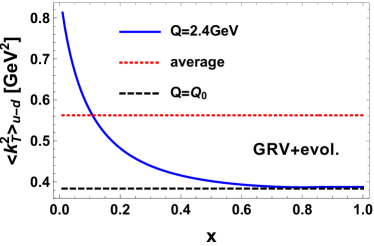
Figure 5: Transverse-momentum width of the $u-d$ TMD in the proton, plotted as a function of the momentum fraction $x$. The model takes a factorized ansatz at the scale $Q_{0}=510$ MeV with the GRV parametrization and carries out the Kwieciński evolution of Eq. (46) to the lattice scale $Q=2.4$ GeV. We notice the broadening of the $k_{T}$ distribution as $Q$ grows or $x$ decreased. The dashed line indicates $\langle k_{T}\rangle_{0}$ originating from the form factor $\hat{F}$ of Eq. (49), whereas the dotted line shows the value at $Q$ averaged over $x$.

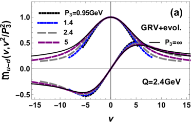
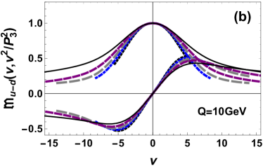
Figure 6: Reduced $u-d$ ITD of the proton at various values of $P_{3}$ at the evolution scale (a) $Q=2.4$ GeV and (b) $Q=10$ GeV, obtained from the model described in the text. The solid line represents the $P_{3}\to\infty$ limit.

The key question we wish to address now is whether the described breaking of the longitudinal-transverse factorization induced by the evolution of the TMDs leads to noticeable effects in ITDs or QDFs at the scales relevant for the present-day lattice studies. We first compare the results for the reduced $u-d$ ITDs following from the evolved distributions, which are shown in Fig. 6. Recall that the external form factor effects (i.e., those coming from $\hat{F}$) cancel out from this quantity Orginos et al. (2017), hence it serves as a probe for the breaking effects due to evolution. The dashed curves, distinguished by the value of $P_{3}$, correspond to the model described above, where the initial condition for the PDF is set at the GRV scale $Q_{0}=510$ MeV, and the Kwieciński evolution is carried out to (a) $Q=2.4$ GeV or (b) $Q=10$ GeV. The solid line shows the $P_{3}\to\infty$ case, where the ITD corresponds to the Fourier transform of the PDF (similarly as the curves in Fig. 3). We note a visible departure from universality, which at $|\nu|=7$ reaches about 30% for $Q=2.4$ GeV and 50% for $Q=10$ GeV for $P_{3}\sim 1$ GeV.

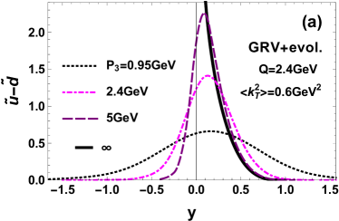
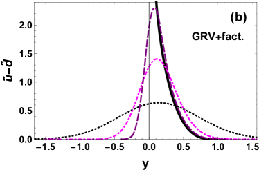
Figure 7: The $\tilde{u}-\tilde{d}$ QDF of the proton at several values of $P_{3}$, obtained from a model with the GRV parameterization of the PDFs at $Q_{0}=510$ MeV, supplied with a Gaussian form factor. In (a) the distributions are evolved to $Q=2.4$ GeV with the Kwieciński equations, whereas in (b) factorization is imposed at the scale $Q$. In both cases the width of the transverse momentum distribution averaged over $x$ is the same and equals $\langle k_{T}^{2}\rangle=0.6~{}{\rm GeV}^{2}$.

Whereas the factorization breaking effects displayed in Fig. 3 seem substantial, or at least relevant at larger values of $|\nu|$, the issue is to what extent they can influence the QDFs. The point here is that the form of Eq. (15) leads to diffusion of the PDF into QDF, which is best seen in the factorized ansatz (36) or (37). In particular, the PDF at low values of $x$, where we would expect more effect from factorization breaking, is diffused more, as the width of the $k_{T}$ distribution is larger in that region. As a result, there is no visible effect on the QDFs from the factorization breaking induces be evolution in our model. This can be seen from Fig. 7, where in panel (a) we show the model with the Kwieciński evolution, which induced the factorization breaking, to be compared with panel (b), which assumes factorization at the final scale of $Q=2.4$ GeV. We note that the two cases lead to essentially identical results. Thus, as advocated in Orginos et al. (2017), the place to look for potential factorization breaking are the ITDs and not the QDFs. Our study supports this conclusion.

VI Comparison to the Euclidean lattice simulations

In this Section we compare our results to QDFs obtained from the ETMC full-QCD lattice simulations reported in Alexandrou et al. (2016). As we have seen that the effects of the transverse-longitudinal factorization seem negligible for QDFs, we return now to the model with the NNPDF distributions used in Sect. IV and the simple Gaussian factorization ansatz (35) taken at the lattice scale $Q=2.4$ GeV.

The results for $P_{3}=1.9$ GeV are shown in Fig. 8, where we use the model with three different values of $\langle k_{T}^{2}\rangle$. We note that the model curves move closer to the PDF as $\langle k_{T}^{2}\rangle$ is being decreased, which is obvious from the discussion below Eq. (36). We recall that the combination $\langle k_{T}^{2}\rangle/P_{3}^{2}$ is the relevant parameter, and its going to zero provides the PDF limit. At the same time, the comparison to the ETMC data, represented with a band, is qualitative only, except perhaps the large-$y$ region for $\langle k_{T}^{2}\rangle=0.6~{}{\rm GeV}^{2}$.

Figure 8 presents a similar study, where we keep $\langle k_{T}^{2}\rangle$ at the value of $0.3~{}{\rm GeV}^{2}$ Bacchetta et al. (2017), but change the value of $P_{3}$. Comparison is made to the corresponding three QDF extractions from the ETMC data, indicated with the bands. Again, the model curves are substantially away from the lattice extractions.

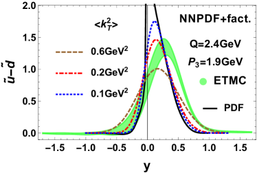
Figure 8: The $\tilde{u}-\tilde{d}$ QDF of the proton in the factorization model with the NNPDF distributions at various values of the width of the $k_{T}$ distribution (lines), compared to the lattice results from ETMC Alexandrou et al. (2016) (band). Both the model results and the ETMC data are for $P_{3}=1.9$ GeV. The solid line shows the PDF, which is the limit of the QDF at $\langle k_{T}^{2}\rangle\to 0$.

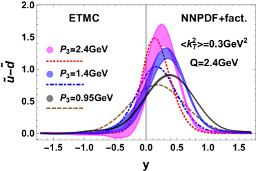
Figure 9: Same as in Fig. 8, but for the case where $\langle k_{T}^{2}\rangle=0.3~{}{\rm GeV}^{2}$ is fixed and $P_{3}$ changed.

There are several possible reasons for the discrepancy. First, as discussed in Appendix A, the extraction of QDF in Alexandrou et al. (2015, 2016, 2017a, ) uses a prescription retaining the structure proportional to $z^{\mu}$. Then, the Radyushkin QDF-TMD relation (11) receives corrections subleading in the twist expansion. Moreover, this choice leads to mixing with a subleading-twist scalar channel which needs to be disentangled Alexandrou et al. (2017b). Another issue is the value of the pion mass, which in the ETMC simulations is $m_{\pi}=370$ MeV. One artifact, possibly caused by a large departure from the physical pion mass limit, is a large value of the momentum fraction $\langle x\rangle_{u-d}=0.23$ (cf. Table I of Alexandrou et al. (2017a)), compared to the phenomenological value of 0.16. Thus, quite naturally, the lattice QDFs are moved to the right from the PDF, as in Figs. 8 and 9. A proper extrapolation in $m_{\pi}$ down to physical value may resolve this problem. The target-mass corrections Alexandrou et al. (2015); Radyushkin (2017b) also move the lattice extractions closer to the data. Apart from the issues mentioned above, there are also typical lattice problems, such as a finite cut-off from the lattice spacing, volume effects, the source-sink separation, etc.

We note that the quenched simulation in Orginos et al. (2017), which served as a proof of concept of the invented methods and where the $P^{0}$ projection discussed in Appendix A was used, the value of the pion mass was 600 MeV. In this study, the PDF extracted from the lattice is also visibly to the right of the phenomenological distribution.

Besides these issues, we note from Fig. 9 that the needed values for $P_{3}$ to achieve a few-percent agreement with the PDF limit for $x>0.15$ are $P_{3}>5~{}{\rm GeV}$, or more appropriately, $\langle k_{T}^{2}\rangle/P_{3}^{2}<0.025$.

Finally, we illustrate in the nucleon case the sum rules discussed in Section III, which for the second central moment (23,27) yield

$$\langle y^{2}\rangle-\langle y\rangle^{2}=\langle x^{2}\rangle-\langle x\rangle^{2}+\frac{\overline{\langle k_{T}^{2}\rangle}}{2P_{3}^{2}}.$$ (50)

This relation allows us to extract the TMD width, $\overline{\langle k_{T}^{2}\rangle}$, directly from the lattice data on QDFs from the ETMC collaboration Alexandrou et al. (2016). We just make a linear fit of the form $A+B/P_{3}^{2}$. The result is depicted in Fig. 10, where a clear straight line can be seen. The slope yields the value of $\langle k_{T}^{2}\rangle_{u-d}=0.27~{}{\rm GeV}^{2}$.  Another determination of this quantity was made in the lattice study Musch et al. (2011) by means of a Gaussian fit in $k_{T}$, with the result $\langle k_{T}^{2}\rangle_{u-d}=(0.16(1)~{}{\rm GeV})^{2}$ at $m_{\pi}=600$ MeV. In addition, we note from Fig. 10 an agreement of the second central $x$ moment with the phenomenological GRV analysis Glück et al. (1998), holding in the range $Q=0.5-2.4{\rm GeV}$, with a better agreement for the lower scale.

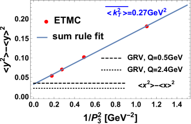
Figure 10: The sum rule of Eq. 50 at work. We use the lattice data from the ETMC collaboration Alexandrou et al. (2016) to compute the second $y$-moment of the QDFs. We note that the value at the origin gives the second central $x$-moment of the PDF. The horizontal lines correspond to the phenomenological GRV analysis Glück et al. (1998) for the values $Q=0.5$ and $2.4~{}{\rm GeV}$. The slope yields the value of $\overline{\langle k_{T}^{2}\rangle}_{u-d}=0.27~{}{\rm GeV}^{2}$ for the spread of the transverse momentum distribution.

VII Predictions for the pion

Finally, we wish to make some predictions for the pion, which undoubtedly also will be soon analyzed on the lattice in the context of ITDs or QDFs. Note that a similar object, namely the pion quasi-distribution amplitude Ji (2013); Radyushkin (2017d), has been evaluated on the lattice Zhang et al. (2017) and reproduced favorably in a chiral quark model Broniowski and Ruiz Arriola (2017).

The phenomenological parton distributions for the pion were extracted from the Drell-Yan and the prompt photon emission experiments. The parametrization provided in Sutton et al. (1992), denoted as SMRS (see Table VII, NA10 case at $Q^{2}=5~{}{\rm GeV}^{2}$), reads

$$V_{\pi}(x)=Ax^{-0.4}(1-x)^{1.08},$$ (51)

for the valence quark PDF of the pion. We use his form to derive, with the techniques of the previous Sections, the corresponding QDF and the reduced ITD.

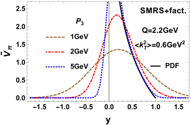
Figure 11: Valence QDFs of the pion at various values of $P_{3}$ for the SMRS parametrization (51). Factorization ansatz is imposed at the scale $Q=2.2$ GeV. The solid line indicates the valence PDF of the pion.

In Fig. 11 we show the valence QDFs of the pion, $V_{\pi}$, at several values of $P_{3}$ in a model, where a Gaussian factorization ansatz of width $\langle k_{T}^{2}\rangle=0.6~{}{\rm GeV}^{2}$ is imposed at the SMRS scale $Q=2.2$ GeV, with the PDF taken from Eq. (51). We note a behavior qualitatively similar to the proton case of Fig. 7, with the QDF converging to within a few percent to the PDF at $P_{3}>5$GeV (for $x>0.15$).

We have also carried out a similar analysis with the factorization breaking in the pion due to the Kwieciński evolution starting from the GRS Gluck et al. (1999) parametrization at the scale of $Q_{0}=510$ MeV and carried out up to $Q=2.2$ GeV, and found small factorization breaking effects in QDFs, similarly to the proton case discussed in detail in Section V.

The longitudinal-transverse factorization breaking due to the QCD evolution naturally increases with the evolution ratio $r\equiv\alpha_{\rm QCD}(Q_{0})/\alpha_{\rm QCD}(Q)$. Thus the effect will be enhanced in approaches where $r$ is large. This is notoriously the case of the chiral quark models ($\chi$QM) (for a review in the context of PDF and PDA analyses, see Ruiz Arriola (2002) and references therein), where the quark-model scale $Q_{0}$ is very low, $Q_{0}\sim 320$ MeV, and $r\simeq 7$ for $Q=2.2$ GeV. The quark-model scale is defined as the scale where the valence quarks, which are the only degrees of freedom in the model, saturate the momentum sum rule.

In Fig 12 we present the reduced valence ITD of the pion, evaluated in $\chi$QM, where the PDF at the initial scale $Q_{0}$ has a constant value Davidson and Ruiz Arriola (1995), and the Kwieciński evolution (46) is performed up to $Q=2.2$ GeV. We notice strong violation effects, larger than for the analogous plot for the nucleon (6), which is a result of an increased evolution ratio $r$. We note that at $|\nu|=5$ the effect reaches 100% for the lower values of $P_{3}$.9

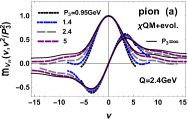
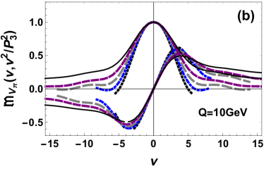
Figure 12: Reduced valence ITD of the pion, evaluated in the Chiral Quark Model ($\chi$QM) at various values of $P_{3}$. At the origin, the real and imaginary parts equal 1 or 0, respectively.

VIII Conclusions

The ab initio determination of the parton distribution functions is a formidably complex problem which remains a pending issue in hadronic structure. Whereas the $x$-moments method has been for a long time the only available scheme for Euclidean lattices, the QDF methodology proposed by Ji has opened a new venue in the field by considering space-like correlators boosted to a finite momentum, and eventually extrapolating to the infinite momentum limit. These apparently auxiliary new mathematical objects have been found by Radyushkin to be intertwined with the well known TMDs, or more generally, with the pseudo-distributions. This makes QDFs at finite longitudinal momentum interesting on their own. As a bonus, this connection suggests a working scheme to implement the QCD evolution for QDFs via an evolution of TMDs, which has been studied for many years, offering working prescriptions ready to use.

In the present paper we have profited from the Radyushkin relation between the QDFs and TMDs or ITDs in several ways. First, we have written down some useful sum rules which can be easily used as consistency checks for the lattice studies. The sum rules show that at low values of the Ioffe time, the reduced ITDs are essentially dominated with the lowest $x$-moments of PDFs. Application of the sum rules to ITDs also allows one, with sufficiently accurate lattice data, for an extraction of the transverse-momentum widths of TMDs. We have checked favorably the lowest sum rule on the ETMC lattice data and obtained the $k_{T}$-width of the TMD of the nucleon at a low scale.

Second, we have conducted a phenomenological analysis of the QCD evolution effects on the quark and gluon components of the proton using the Kwieciński extension of the one-loop CCFM equations. Our method uses the established parameterizations of PDFs in conjunction with the widely employed longitudinal-transverse factorization ansatz imposed at a low momentum scale. We have focused on the examination of the factorization breaking due to the QCD evolution. While, strictly speaking, the factorization ansatz can only hold at a given reference scale, we have shown that the breaking of factorization is not numerically very large as long as the evolution ratio is not large. Whereas the breaking is visible in the reduced ITDs, it essentially disappears from QDFs at the presently available scales. This finding is in agreement with factorization studies on the lattice, where factorization is found to hold in a relatively wide range. The reason is due to a rather weak effect of the QCD evolution at the scales presently available on the lattice. All these results make the a priori naive but actually valid factorization property even more intriguing from a theoretical point of view.

Finally, we have presented predictions for the valence-quark QDF in the pion, as well as for the corresponding reduced ITD. To enhance the possible effects of the longitudinal-transverse factorization breaking, we have used chiral quark models, where the QCD evolution ration is large and the effect are largely enhanced. This calculation may serve as a limit of how large the breaking effects could be.

Appendix A Decomposition of the matrix element

Rewriting Eq. (1) for brevity as

$$M^{\mu}=P^{\mu}A+z^{\mu}B,$$ (52)

we find from contractions with $P_{\mu}$ and $z_{\mu}$ the relations

$$A=\frac{M\cdot z\,P\cdot z-M\cdot p\,z^{2}}{P\cdot z^{2}-P^{2}z^{2}},$$

$$B=\frac{M\cdot p\,P\cdot z-M\cdot z\,P^{2}}{P\cdot z^{2}-P^{2}z^{2}}.$$ (53)

We may now consider the kinematic cases of interest. For PDFs, the only nonzero component of $z$ is $z^{-}$, hence taking $\gamma^{+}$ in the definition (1) yields

$$M^{+}=P^{+}A.$$ (54)

The same relation holds for TMDs, where $z^{-}$ and $z_{T}$ are nonzero. For the kinematics of QDFs defined by Ji Ji (2013), only $z^{3}$ is nonzero, and

$$M^{3}=P^{3}A+z^{3}B,$$ (55)

where both $A$ and $B$ structures enter, precluding a generic link to TMD, which contains $A$ only. In Ref. Orginos et al. (2017) it is proposed to take

$$M^{0}=P^{0}A.$$ (56)

Note that despite the mixing in Eq. (55), in the limit of $P_{3}\to\infty$ (under assumptions of regularity of $B$), the term with $A$ dominates, hence the asymptotic link to the PDF follows.

We note that in Alexandrou et al. (2015, 2016, 2017a, ) the $M^{3}$ prescription is used, hence the above difficulty arises. Moreover, this choice leads to mixing of the unpolarized QDF with the twist-3 scalar correlator Alexandrou et al. (2017b), adding to technical difficulties.

One could also use the prescription with $M^{3}$, but with $z$ having only a non-vanishing transverse component, $z_{2}$. In that case $M^{3}=P^{3}A$.

Appendix B Transversity relation for the pion wave function

Consider the relation Broniowski et al. (2010)

$$\Psi_{a}(P\cdot z,z^{2})=\int_{0}^{1}d\alpha e^{i(2\alpha-1)P\cdot z}\Phi_{a}(\alpha,z^{2}),$$ (57)

where $\Psi_{a}(z\cdot q,z^{2})$ is the pion wave function (related to the Bethe-Salpeter amplitude in the given tensor channel $a$), and $\Phi_{a}(z\cdot q,z^{2})$ is its Fourier transform. The functions, as Lorentz invariants, depend on the two available scalars $P\cdot z$ and $z^{2}$. Choosing two specific frames: equal-time (ET), with $z=(0,\vec{r})$ and $P=(m_{\pi},0)$, and the infinite-momentum light-cone frame (LC), with $z_{+}=0$ and $P=(P_{0},0,0,P_{3})=\lim_{P_{3}\to\infty}(\sqrt{m_{\pi}^{2}+P_{3}^{2}},0,0,P_{3})$, hence $P_{+}z_{-}=P\cdot z=0$, one derives a relation between the ET and LC pion wave functions

$$\Psi^{\rm ET}_{a}(0,-r^{2})=\int_{0}^{1}d\alpha\Phi^{\rm LC}_{a}(\alpha,-r^{2}).$$ (58)

The integration variable $\alpha$ in Eq. (58) acquires the meaning of the light-cone momentum fraction of the pion carried by the quark.

We bring up this example, since the discussion in this paper concerning the distribution functions bears a lot of similarity. In that case, direct analogs of $\Phi_{a}(\alpha,z^{2})$ are the pseudo-distributions introduced by Radyushkin Radyushkin (2017c).

Appendix C Derivation of the Radyushkin relation

In this Appendix we present, for completeness, a pedestrian derivation of Eq. (11), which is based solely on the Lorentz invariance Radyushkin (2017c) of the matrix element $h$ appearing in the decomposition (1).

In the definition of TMD we encounter, by construction, the matrix element

$$h(P\cdot z,z^{2})|_{z_{+}=0}=h(P_{+}z_{-},-z_{1}^{2}-z_{2}^{2}),$$ (59)

whereas in QDF

$$h(P\cdot z,z^{2})|_{z_{0}=0,z_{1}=z_{2}=0}=h(-P_{3}z_{3},-z_{3}^{2}).$$ (60)

Now, following Radyushkin (2017c), one takes the specific value

$$k_{2}=(x-y)P_{3}$$ (61)

in the definition (8). Then, using Eq. (8) and carrying out the two integrations from Eq. (11) we readily find

$$\int\!\!dk_{1}\!\!\int\!\!dx\,q(x,k_{1},(y-x)P_{3})=P^{+}\!\!\!\int dz^{-}\delta(P_{+}z_{-}+P_{3}z_{2})$$

$$~{}~{}~{}\times\int dz_{1}\delta(z_{1})\!\!\!\int\frac{dz_{2}}{2\pi}e^{-iyP_{3}z_{2}}h(P_{+}z_{-},-z_{1}^{2}-z_{2}^{2})=$$

$$~{}~{}~{}\int\frac{dz_{2}}{2\pi}e^{-iyP_{3}z_{2}}h(-P_{3}z_{2},-z_{2}^{2})=$$

$$~{}~{}~{}\int\frac{dz_{3}}{2\pi}e^{-iyP_{3}z_{3}}h(-P_{3}z_{3},-z_{3}^{2})\equiv\frac{1}{P_{3}}\tilde{q}(y,P_{3}).$$ (62)

Since the support of $q(x,k_{T})$ is $x\in[-1,1]$, the $x$ integration can be formally carried in $(-\infty,\infty)$, yielding the delta function. In the last line we have changed the notation for the dummy integration variable, $z_{2}\to z_{3}$, which finally yields Eq. (11).

References

- Collins (2013) J. Collins, Foundations of perturbative QCD (Cambridge University Press, 2013).
- Burkardt and Seal (2002) M. Burkardt and S. K. Seal, Phys. Rev. D65, 034501 (2002), arXiv:hep-ph/0102245 [hep-ph] .
- Dalley and van de Sande (2003) S. Dalley and B. van de Sande, Phys. Rev. D67, 114507 (2003), arXiv:hep-ph/0212086 [hep-ph] .
- Burkardt and Dalley (2002) M. Burkardt and S. Dalley, Prog. Part. Nucl. Phys. 48, 317 (2002), arXiv:hep-ph/0112007 [hep-ph] .
- Musch et al. (2011) B. U. Musch, P. Hagler, J. W. Negele, and A. Schafer, Phys. Rev. D83, 094507 (2011), arXiv:1011.1213 [hep-lat] .
- Ji (2013) X. Ji, Phys. Rev. Lett. 110, 262002 (2013), arXiv:1305.1539 [hep-ph] .
- Xiong et al. (2014) X. Xiong, X. Ji, J.-H. Zhang, and Y. Zhao, Phys. Rev. D90, 014051 (2014), arXiv:1310.7471 [hep-ph] .
- Ji (2014) X. Ji, Sci. China Phys. Mech. Astron. 57, 1407 (2014), arXiv:1404.6680 [hep-ph] .
- Ma and Qiu (2014) Y.-Q. Ma and J.-W. Qiu, (2014), arXiv:1404.6860 [hep-ph] .
- Ji and Zhang (2015) X. Ji and J.-H. Zhang, Phys. Rev. D92, 034006 (2015), arXiv:1505.07699 [hep-ph] .
- Ji et al. (2015) X. Ji, A. Schäfer, X. Xiong, and J.-H. Zhang, Phys. Rev. D92, 014039 (2015), arXiv:1506.00248 [hep-ph] .
- Radyushkin (2017a) A. Radyushkin, Phys. Lett. B767, 314 (2017a), arXiv:1612.05170 [hep-ph] .
- Monahan and Orginos (2017) C. Monahan and K. Orginos, JHEP 03, 116 (2017), arXiv:1612.01584 [hep-lat] .
- Chen et al. (2017) J.-W. Chen, X. Ji, and J.-H. Zhang, Nucl. Phys. B915, 1 (2017), arXiv:1609.08102 [hep-ph] .
- Ji et al. (2017) X. Ji, J.-H. Zhang, and Y. Zhao, Nucl. Phys. B924, 366 (2017), arXiv:1706.07416 [hep-ph] .
- Chen et al. (2018) J.-W. Chen, T. Ishikawa, L. Jin, H.-W. Lin, Y.-B. Yang, J.-H. Zhang, and Y. Zhao, Phys. Rev. D97, 014505 (2018), arXiv:1706.01295 [hep-lat] .
- Carlson and Freid (2017) C. E. Carlson and M. Freid, Phys. Rev. D95, 094504 (2017), arXiv:1702.05775 [hep-ph] .
- Briceño et al. (2017) R. A. Briceño, M. T. Hansen, and C. J. Monahan, Phys. Rev. D96, 014502 (2017), arXiv:1703.06072 [hep-lat] .
- Rossi and Testa (2017) G. C. Rossi and M. Testa, Phys. Rev. D96, 014507 (2017), arXiv:1706.04428 [hep-lat] .
- Stewart and Zhao (2017) I. W. Stewart and Y. Zhao, (2017), arXiv:1709.04933 [hep-ph] .
- Radyushkin (2017b) A. Radyushkin, Phys. Lett. B770, 514 (2017b), arXiv:1702.01726 [hep-ph] .
- Alexandrou et al. (2015) C. Alexandrou, K. Cichy, V. Drach, E. Garcia-Ramos, K. Hadjiyiannakou, K. Jansen, F. Steffens, and C. Wiese, Phys. Rev. D92, 014502 (2015), arXiv:1504.07455 [hep-lat] .
- Alexandrou et al. (2016) C. Alexandrou, K. Cichy, M. Constantinou, K. Hadjiyiannakou, K. Jansen, F. Steffens, and C. Wiese, Proceedings, 34th International Symposium on Lattice Field Theory (Lattice 2016): Southampton, UK, July 24-30, 2016, PoS LATTICE2016, 151 (2016), arXiv:1612.08728 [hep-lat] .
- Alexandrou et al. (2017a) C. Alexandrou, K. Cichy, M. Constantinou, K. Hadjiyiannakou, K. Jansen, F. Steffens, and C. Wiese, Phys. Rev. D96, 014513 (2017a), arXiv:1610.03689 [hep-lat] .
- (25) C. Alexandrou, S. Bacchio, K. Cichy, M. Constantinou, K. Hadjiyiannakou, K. Jansen, G. Koutsou, A. Scapellato, and F. Steffens, in 35th International Symposium on Lattice Field Theory (Lattice 2017) Granada, Spain, June 18-24, 2017.
- Orginos et al. (2017) K. Orginos, A. Radyushkin, J. Karpie, and S. Zafeiropoulos, Phys. Rev. D96, 094503 (2017), arXiv:1706.05373 [hep-ph] .
- Gamberg et al. (2015) L. Gamberg, Z.-B. Kang, I. Vitev, and H. Xing, Phys. Lett. B743, 112 (2015), arXiv:1412.3401 [hep-ph] .
- Miller and Tiburzi (2010) G. A. Miller and B. C. Tiburzi, Phys. Rev. C81, 035201 (2010), arXiv:0911.3691 [nucl-th] .
- Broniowski et al. (2010) W. Broniowski, S. Prelovsek, L. Santelj, and E. Ruiz Arriola, Phys. Lett. B686, 313 (2010), arXiv:0911.4705 [hep-ph] .
- Ruiz Arriola and Broniowski (2010) E. Ruiz Arriola and W. Broniowski, Proceedings, International Workshop on Relativistic hadronic and particle physics (Light Cone 2010): Valencia, Spain, June 14-18, 2010, PoS LC2010, 041 (2010), arXiv:1009.5781 [hep-ph] .
- Miller (2010) G. A. Miller, Ann. Rev. Nucl. Part. Sci. 60, 1 (2010), arXiv:1002.0355 [nucl-th] .
- Radyushkin (2017c) A. V. Radyushkin, Phys. Rev. D96, 034025 (2017c), arXiv:1705.01488 [hep-ph] .
- Radyushkin (2017d) A. V. Radyushkin, Phys. Rev. D95, 056020 (2017d), arXiv:1701.02688 [hep-ph] .
- Radyushkin (2017e) A. V. Radyushkin, (2017e), arXiv:1710.08813 [hep-ph] .
- Angeles-Martinez et al. (2015) R. Angeles-Martinez et al., Acta Phys. Polon. B46, 2501 (2015), arXiv:1507.05267 [hep-ph] .
- Ioffe (1969) B. L. Ioffe, Phys. Lett. 30B, 123 (1969).
- Braun et al. (1995) V. Braun, P. Gornicki, and L. Mankiewicz, Phys. Rev. D51, 6036 (1995), arXiv:hep-ph/9410318 [hep-ph] .
- Karpie et al. (2017) J. Karpie, K. Orginos, A. Radyushkin, and S. Zafeiropoulos, (2017), arXiv:1710.08288 [hep-lat] .
- (39) C. Monahan and K. Orginos, in 35th International Symposium on Lattice Field Theory (Lattice 2017) Granada, Spain, June 18-24, 2017.
- D’Alesio and Murgia (2004) U. D’Alesio and F. Murgia, Phys. Rev. D70, 074009 (2004), arXiv:hep-ph/0408092 [hep-ph] .
- Schweitzer et al. (2010) P. Schweitzer, T. Teckentrup, and A. Metz, Phys. Rev. D81, 094019 (2010), arXiv:1003.2190 [hep-ph] .
- Ciafaloni (1988) M. Ciafaloni, Nucl. Phys. B296, 49 (1988).
- Catani et al. (1990a) S. Catani, F. Fiorani, and G. Marchesini, Phys. Lett. B234, 339 (1990a).
- Catani et al. (1990b) S. Catani, F. Fiorani, and G. Marchesini, Nucl. Phys. B336, 18 (1990b).
- Kwiecinski (2002) J. Kwiecinski, Acta Phys. Polon. B33, 1809 (2002), arXiv:hep-ph/0203172 [hep-ph] .
- Gawron and Kwiecinski (2003) A. Gawron and J. Kwiecinski, Acta Phys. Polon. B34, 133 (2003), arXiv:hep-ph/0207299 [hep-ph] .
- Gawron et al. (2003) A. Gawron, J. Kwiecinski, and W. Broniowski, Phys. Rev. D68, 054001 (2003), arXiv:hep-ph/0305219 [hep-ph] .
- Ruiz Arriola and Broniowski (2004) E. Ruiz Arriola and W. Broniowski, Phys. Rev. D70, 034012 (2004), arXiv:hep-ph/0404008 [hep-ph] .
- Jaffe (1983) R. L. Jaffe, Nucl. Phys. B229, 205 (1983).
- Jaffe (1985) R. L. Jaffe, in Proceedings, Research Program at CEBAF I: Report of the 1985 Summer Study Group, June 10 - August 30, 1985 (1985).
- Ji (1998) X.-D. Ji, J. Phys. G24, 1181 (1998), arXiv:hep-ph/9807358 [hep-ph] .
- Boer et al. (2011) D. Boer, L. Gamberg, B. Musch, and A. Prokudin, JHEP 10, 021 (2011), arXiv:1107.5294 [hep-ph] .
- Bacchetta et al. (2008) A. Bacchetta, F. Conti, and M. Radici, Phys. Rev. D78, 074010 (2008), arXiv:0807.0323 [hep-ph] .
- Wakamatsu (2009) M. Wakamatsu, Phys. Rev. D79, 094028 (2009), arXiv:0903.1886 [hep-ph] .
- Weigel et al. (1999) H. Weigel, E. Ruiz Arriola, and L. P. Gamberg, Nucl. Phys. B560, 383 (1999), hep-ph/9905329 .
- Ruiz Arriola and Broniowski (2003a) E. Ruiz Arriola and W. Broniowski, in Light cone physics: Hadrons and beyond: Proceedings. 2003 (2003) arXiv:hep-ph/0310044 [hep-ph] .
- Ruiz Arriola and Broniowski (2003b) E. Ruiz Arriola and W. Broniowski, Phys. Rev. D67, 074021 (2003b), arXiv:hep-ph/0301202 [hep-ph] .
- Noguera and Scopetta (2015) S. Noguera and S. Scopetta, JHEP 11, 102 (2015), arXiv:1508.01061 [hep-ph] .
- Melis (2015) S. Melis, Proceedings, 4th International Workshop on Transverse Polarization Phenomena in Hard Processes (Transversity 2014): Cagliari, Italy, June 9-13, 2014, EPJ Web Conf. 85, 01001 (2015), arXiv:1412.1719 [hep-ph] .
- Bacchetta et al. (2017) A. Bacchetta, F. Delcarro, C. Pisano, M. Radici, and A. Signori, JHEP 06, 081 (2017), arXiv:1703.10157 [hep-ph] .
- Ball et al. (2013) R. D. Ball et al., Nucl. Phys. B867, 244 (2013), arXiv:1207.1303 [hep-ph] .
- Broniowski et al. (2008) W. Broniowski, E. Ruiz Arriola, and K. Golec-Biernat, Phys.Rev. D77, 034023 (2008), arXiv:0712.1012 [hep-ph] .
- Gribov and Lipatov (1972) V. N. Gribov and L. N. Lipatov, Sov. J. Nucl. Phys. 15, 438 (1972), [Yad. Fiz.15,781(1972)].
- Dokshitzer (1977) Y. L. Dokshitzer, Sov. Phys. JETP 46, 641 (1977), [Zh. Eksp. Teor. Fiz.73,1216(1977)].
- Altarelli and Parisi (1977) G. Altarelli and G. Parisi, Nucl. Phys. B126, 298 (1977).
- Lipatov (1976) L. N. Lipatov, Sov. J. Nucl. Phys. 23, 338 (1976), [Yad. Fiz.23,642(1976)].
- Kuraev et al. (1977) E. A. Kuraev, L. N. Lipatov, and V. S. Fadin, Sov. Phys. JETP 45, 199 (1977), [Zh. Eksp. Teor. Fiz.72,377(1977)].
- Balitsky and Lipatov (1978) I. I. Balitsky and L. N. Lipatov, Sov. J. Nucl. Phys. 28, 822 (1978), [Yad. Fiz.28,1597(1978)].
- Golec-Biernat et al. (2007) K. J. Golec-Biernat, S. Jadach, W. Placzek, P. Stephens, and M. Skrzypek, Acta Phys. Polon. B38, 3149 (2007), arXiv:hep-ph/0703317 [hep-ph] .
- Gustafson et al. (2002) G. Gustafson, L. Lonnblad, and G. Miu, JHEP 09, 005 (2002), arXiv:hep-ph/0206195 [hep-ph] .
- Glück et al. (1998) M. Glück, E. Reya, and A. Vogt, Eur. Phys. J. C5, 461 (1998), arXiv:hep-ph/9806404 [hep-ph] .
- Alexandrou et al. (2017b) C. Alexandrou, K. Cichy, M. Constantinou, K. Hadjiyiannakou, K. Jansen, H. Panagopoulos, and F. Steffens, Nucl. Phys. B923, 394 (2017b), arXiv:1706.00265 [hep-lat] .
- Zhang et al. (2017) J.-H. Zhang, J.-W. Chen, X. Ji, L. Jin, and H.-W. Lin, Phys. Rev. D95, 094514 (2017), arXiv:1702.00008 [hep-lat] .
- Broniowski and Ruiz Arriola (2017) W. Broniowski and E. Ruiz Arriola, Phys. Lett. B773, 385 (2017), arXiv:1707.09588 [hep-ph] .
- Sutton et al. (1992) P. J. Sutton, A. D. Martin, R. G. Roberts, and W. J. Stirling, Phys. Rev. D45, 2349 (1992).
- Gluck et al. (1999) M. Gluck, E. Reya, and I. Schienbein, Eur. Phys. J. C10, 313 (1999), hep-ph/9903288 .
- Ruiz Arriola (2002) E. Ruiz Arriola, 42nd Cracow School of Theoretical Physics: 42nd Course 2002: Flavor Dynamics Zakopane, Poland, May 31-June 9, 2002, Acta Phys. Polon. B33, 4443 (2002), arXiv:hep-ph/0210007 [hep-ph] .
- Davidson and Ruiz Arriola (1995) R. Davidson and E. Ruiz Arriola, Phys.Lett. B348, 163 (1995).